OM-II, Chapter 2(Slides) AIM

8/8/2019 OM-II, Chapter 2(Slides) AIM

http://slidepdf.com/reader/full/om-ii-chapter-2slides-aim 1/41

© Nigel Slack, Stuart Chambers & Robert John ston, 2004

• What are the advantages of holding

inventory?

• What are the disadvantages?

Inventory Management




Day-to-day Inventory Decision

• To maintain the appropriate level of

inventory, operations managers are involved

in 2 major types of decision:

1. Volume decision: How much to order?

2. Timing decisions: When to order?




The order quantity decision

Stock-holdingcosts

Orderingcosts

How much

to order?




The economic order quantity

Order quantity (Q)

Inventory Ordering Costs

Inventory carrying costs

Total costs

EOQ

Costs(

$)

Cost Curves: Graphical relationship between various costs




Economic Order Quantity: Optimising Tradeoffs

Ordering More Frequently Ordering Less Frequently

• Higher Ordering Costs • Lower Ordering Costs

• Smaller Average Inventory • Larger Average Inventory

Need to Calculate:

CO = fixed cost of placing an order

CH = holding cost per item per unit of time (e.g. a year)

Aim is to minimise ordering and holding costs




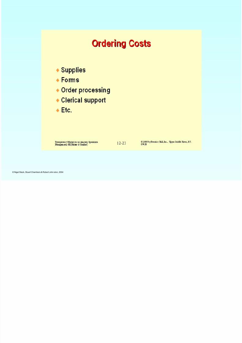
D. Economic Order Quantity

(EOQ) Model• Developed by F.W. Harris, 1913

• Answers two key questions

– when to order

– how much to order

• Independent demand, continuous review

system




Inventory Cycle

Time

InventoryLevel

OrderQuantity

ReorderPoint

Q

RP

Lead-timeLT

}

Slope

-D




Reorder Point

• Inventory level should reach 0 at end of each

order cycle

• RP equals demand during lead-time (DDLT)

RP = DDLT = D x LT

D = demand

LT = lead-timeD & LT must be in same time units




Computing Optimal Order Quantity

• Compute total material cost, TMC

• TMC is a function of order quantity, Q

Ordering costs, co[D/Q]Holding costs, c

h[Q/2]

Variable item costs, pD

TMC = co[D/Q] + c

h[Q/2] + pD




Total Stocking Cost

• pD is constant, no quantity discounts

• TSC = ordering + holding

= co[D/Q] + ch[Q/2]

• Find Q to minimize TSC

EOQ= 2ocDhc




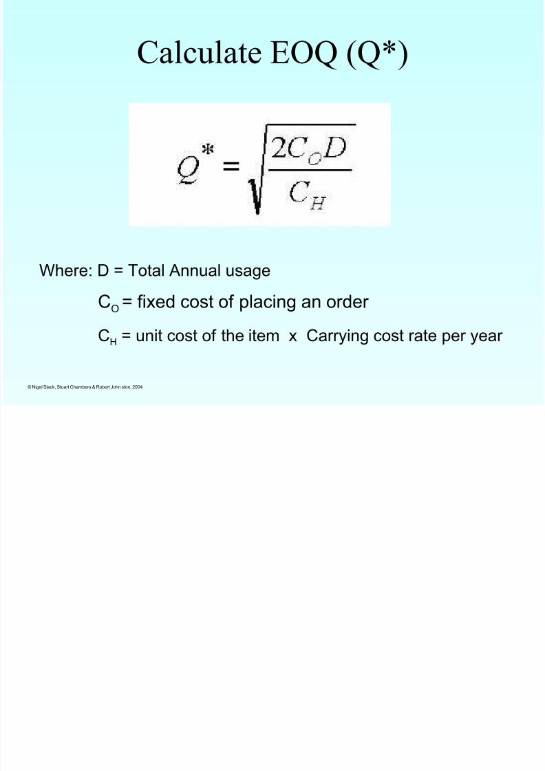
Calculate EOQ (Q*)

Where: D = Total Annual usage

CO = fixed cost of placing an order

CH = unit cost of the item x Carrying cost rate per year




Fastcomp Example

p = $80

co= $1000

i = 12% per year

D = 10,000 chips per month

LT = 1.5 months

RP = 10,000 units/month x 1.5 months = 15,000 units

ch

= p x i = $80 x 0.12/year = $9.60/unit-year




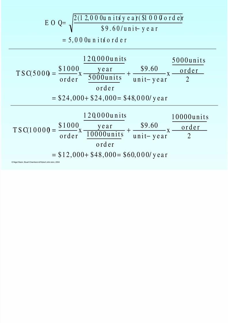
T S C(5 0 0 0) =$ 1 0 0 0

o r d e r

x

1 2 0, 0 0 0 u n its

y e a r

5 0 0 0 u n i t so r d e r

+$9.60

u n i t− y e a r

x

5 0 0 0 u n i t s

o r d e r

2

= $ 2 4 , 0 0 0+ $ 2 4 , 0 0 0= $ 4 8, 0 0 0/ y e a r

T S C(1 0 0 0 0) =$ 1 0 0 0

o r d e rx

1 2 0, 0 0 0 u n i ts

y e a r1 0 0 0 0 u n i t s

o r d e r

+$9.60

u n i t− y e a rx

1 0 0 0 0 u n i t so r d e r

2

= $ 1 2 , 0 0 0+ $ 4 8 , 0 0 0= $ 6 0, 0 0 0/ y e a r

E O Q=2 (1 2, 0 0 0u n i t s/ y e a r) ( $1 0 0 0/ o r d e r)

$ 9 . 6 0 / u n i t− y e a r

= 5, 0 0 0u n i t s/ o r d e r




Validity Of Assumptions

• Model is quite robust

• Quantity discounts, demand/LT uncertainty,

no stockout assumptions easily relaxed

• Constant demand & holding cost can be

violated somewhat with minor cost penalty

• Total cost function flat near optimum• c

o& c

herrors tend to cancel out




E. EOQ Model With Quantity

Discounts• Quantity discounts offered to encourage

volume purchasing

• RP is not affected by quantity discounts




Revised Cost Model

total material cost/year=

ordering cost + holding cost + item cost

Price is function of Q, p(Q)Holding cost , c

h(Q) = p(Q) x i

Select Q to minimize

TMC = co[D/Q] + [ch(Q)][Q/2] + p(Q)D




Quantity Discount Structure

# Units Purchased Price/Unit

0 < Q < Q1 p1

Q1 ≤ Q < Q2 p2

Q2 ≤ Q < Q3 p3

Q3 ≤ Q p4

where p1 > p2 > p3 > p4




Characteristics Of Cost Functions

• Between any two price-break quantities,

annual item cost is constant because price is

constant within that range

• Annual holding cost function is not straight.

• Between any two price-break qty function

is linear. At price-break qty

(a) total holding cost drops discontinuously

(b) slope of holding cost function decreases




Costs With Quantity Discount

Q1 Q2 Q3

Cost

Total MaterialCost

Item Cost

Holding cost

Ordering Cost




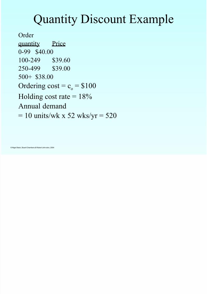
Quantity Discount Example

Order quantity Price

0-99 $40.00

100-249 $39.60

250-499 $39.00

500+ $38.00

Ordering cost = co = $100

Holding cost rate = 18%

Annual demand= 10 units/wk x 52 wks/yr = 520




1. Start at $38 ch = 38x.18 = 6.84

inconsistent with $38 price

2. Select $39 ch = 39x.18 = 7.02

inconsistent with $39 price

Now use $39.60 ch = 39.60x 18 =7.128

consistent with $39.60 price

3. Compute TMC for 121, 250 & 500 units

TMC121 = 100x(520/121)+7.128x(121/2)+39.60x520

= $21,452.99TMC250 = $21,36.54 TMC500 = $21,574.00

250 is optimal order quantity

Q̂= 2x100x520 /6.84 =123

Q̂=

2x100x520 /7.02=

122

Q̂= 2x100x520 /7.128 =121




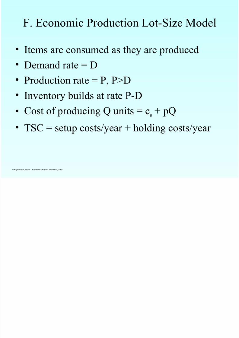
F. Economic Production Lot-Size Model

• Items are consumed as they are produced

• Demand rate = D

• Production rate = P, P>D• Inventory builds at rate P-D

• Cost of producing Q units = co+ pQ

• TSC = setup costs/year + holding costs/year




Production Lot Size Inventory

Pattern

.

Time

Imax= (P-D)Q/P

Slope-D

I

n v e n t o r y L e v

e l

SlopeP-D

Q/P




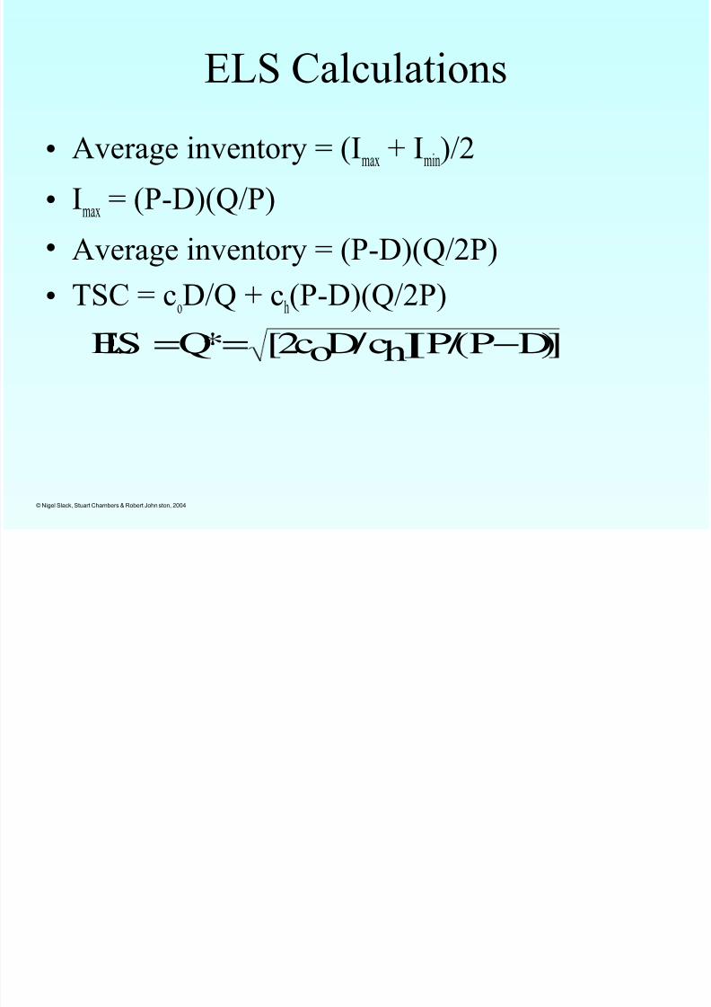
ELS Calculations

• Average inventory = (Imax

+ Imin

)/2

• Imax

= (P-D)(Q/P)

• Average inventory = (P-D)(Q/2P)• TSC = c

oD/Q + c

h(P-D)(Q/2P)

ELS =Q*= [2coD/ch][P/(P−D)]




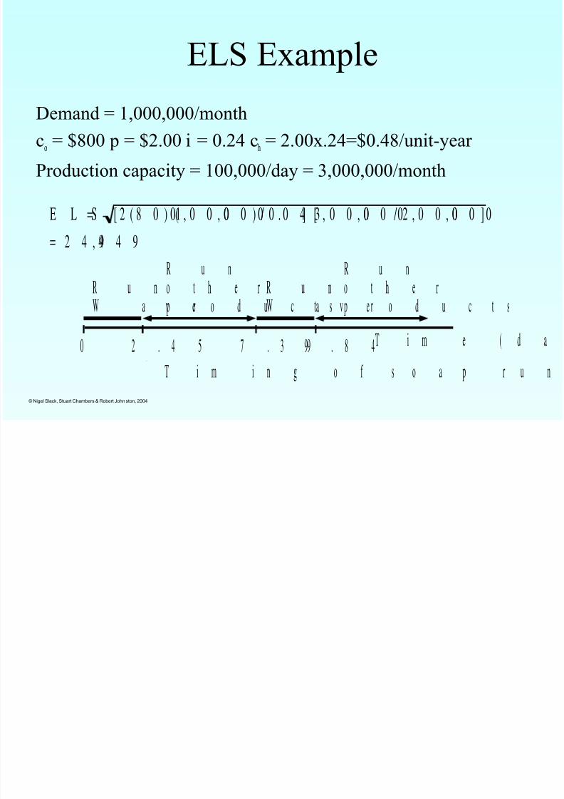
ELS Example

Demand = 1,000,000/month

co= $800 p = $2.00 i = 0.24 c

h= 2.00x.24=$0.48/unit-year

Production capacity = 100,000/day = 3,000,000/month

E L S= [ 2 ( 8 0 0) (1 , 0 0 0, 0 0 0) / 0 . 0 4] [3 , 0 0 0, 0 0 0 / 2 , 0 0 0, 0 0 0]

= 2 4 4, 9 4 9

R u nW a v e

R u no t h e rp r o d u c t s

0 2 . 4 5 7 . 3 99 . 8 4

R u nW a v e

R u no t h e rp r o d u c t s

T i m e ( d a

T i m i n g o f s o a p r u n




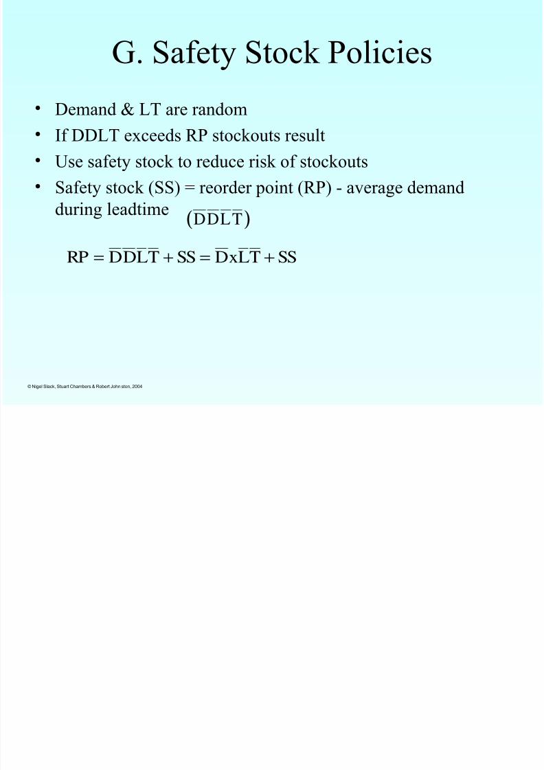
G. Safety Stock Policies

• Demand & LT are random

• If DDLT exceeds RP stockouts result

• Use safety stock to reduce risk of stockouts

• Safety stock (SS) = reorder point (RP) - average demandduring leadtime

DDL T( )

RP = D D L T +SS = D xL T + SS




Inventory Pattern With Random

Demand & Lead Time

Time

RP

Invent

oryLe

vel

Leadtime

Out of stock

Leadtime




The order timing decision

Orderingtoo early

When to

order?

Orderingtoo late




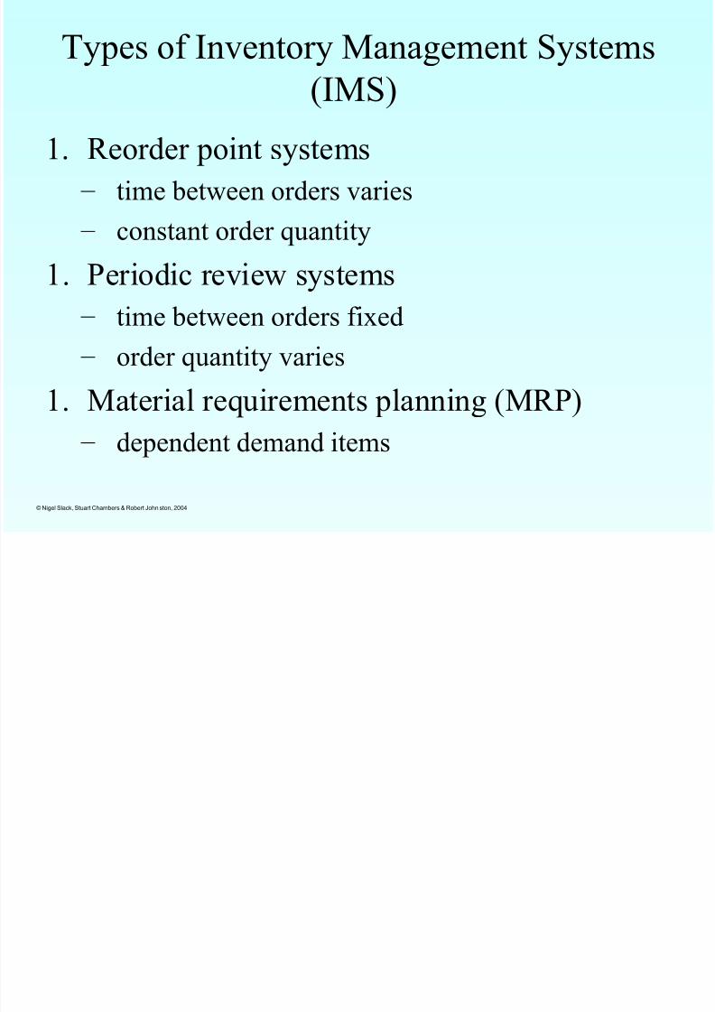
Types of Inventory Management Systems

(IMS)

1. Reorder point systems

– time between orders varies

– constant order quantity

1. Periodic review systems

– time between orders fixed

– order quantity varies

1. Material requirements planning (MRP)

– dependent demand items




Reorder Point System

• In reorder point system an inventory level

is specified at which a replenishment

order for a fixed quantity of the inventory

item is to be placed.




A Reorder Point System




Stock Control Exercise

• Pete noted that stocks were exactly at the maximumstock level of 30,000 units

• It takes 8 days between placing a reorder with the

supplier and the stock actually arriving (i.e. the leadtime is 8 days)

• If stocks must not fall below 12,000 units and if 1000stocks are used each day

– What must Pete set his re-order level at?

– How much must he reorder?




Periodic Review System

• In periodic review system the inventory

level is reviewed periodically and at each

review a reorder may be placed to bring the

level up to a desired quantity.• Reorder quantity

= maximum level – on-hand inventory – on-order

quantity (Q) + demand over lead time




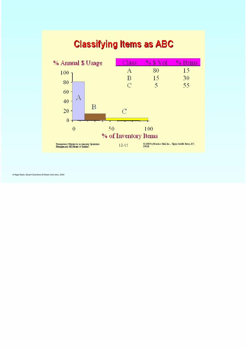
Priorities for Inventory Management:

The ABC Concept

• A. High-value items

– The 15-20% of items that account for 75-80% of annual inventory

value

• B. Medium-value items

– The 30-40% of items that account for15% of annual inventory value

• C. Low-value items

– The 40-50% of items that account for 10-15% of annual inventory

value

The ABC classification system is based on the annual dollar purchases

of an inventoried item

OM-II, Chapter 2(Slides) AIM

Documents

Transcript of OM-II, Chapter 2(Slides) AIM