OLeary Thesis 2011

1

Optic Nerve Head Image

Analysis for Glaucoma

Progression Detection

NEIL O’LEARY

PhD Thesis

Department of Optometry and Visual Science

School of Community and Health Sciences

May 2011

2

Contents List of Tables .......................................................................................................................... 5

List of Figures ........................................................................................................................ 7

Acknowledgements ............................................................................................................ 17

Declaration ........................................................................................................................... 18

Keywords ............................................................................................................................. 19

Abstract................................................................................................................................. 20

List of Abbreviations and Terms ...................................................................................... 21

1. Background and Aims .................................................................................................... 22

1.1 Glaucoma ................................................................................................................... 22

1.1 Diagnostic Technology in Glaucoma ..................................................................... 36

1.2 Confocal Scanning Laser Tomography .................................................................. 41

1.3 Glaucoma Progression.............................................................................................. 54

1.3.1 Heidelberg Retina Tomograph Progression Detection Algorithms............ 56

1.3.2 Assessing the Performance of Change Detection Algorithms ..................... 61

1.4 Objectives ................................................................................................................... 62

2. Glaucomatous Progression in Series of Stereoscopic Photographs and Confocal

Scanning Laser Tomograph Images ................................................................................. 64

2.2 Methods ...................................................................................................................... 66

2.2.1 Patients ................................................................................................................ 66

2.2.2 Selection Criteria for Study ............................................................................... 68

2.2.3 Stereo Optic Disc Photography and Grading ................................................ 68

2.2.4 Confocal Scanning Laser Tomography ........................................................... 70

2.2.5 Statistic Image Mapping ................................................................................... 70

2.2.6 Topographic Change Analysis ......................................................................... 71

2.2.7 Linear Regression of Rim Area ........................................................................ 71

2.2.8 Analysis: Measures of Change and Sliding Scale .......................................... 72

2.4 Results ......................................................................................................................... 73

3

2.5 Discussion .................................................................................................................. 82

3. Trend Detection in Series of Univariate Measurements ............................................ 89

3.1 Trend Detection Techniques .................................................................................... 94

3.2 Data ............................................................................................................................. 98

3.2.1 Real Data ............................................................................................................. 98

3.2.2 Simulated Data ................................................................................................. 100

3.2.2.1 Linear Trend and Stable Data ................................................................. 101

3.2.2.2 Measurement Noise Distribution .......................................................... 102

3.2.2.3 Measurement Variability Levels ............................................................ 104

3.2.2.4 Changes in Within-Series Variability .................................................... 105

3.3 Performance Measures of Change Detection Techniques ................................. 109

3.3.1 Statistical Power ............................................................................................... 110

3.3.2 ROC and Partial ROC Analysis ...................................................................... 110

3.3.3 Imaging Follow-up Period .............................................................................. 112

3.3.4 Students t-Distribution for RA Series Test Statistic ..................................... 112

3.4 Results ....................................................................................................................... 113

3.5 Discussion ................................................................................................................ 123

4. Assessment of Quality in HRT Images ...................................................................... 128

4.1 Measurements of Image Variability ..................................................................... 134

4.1.1 Real Data ........................................................................................................... 134

4.1.2 Simulated Data ................................................................................................. 136

4.2 Measurements of Image Characteristics .............................................................. 141

4.2.1 Image Frequency Analysis .............................................................................. 141

4.2.2 Image Gradient Analysis ................................................................................ 145

4.2.3 Subjective Assessment ..................................................................................... 147

4.3 Results ....................................................................................................................... 148

4.4 Discussion ................................................................................................................ 157

5. Simulation of Series of Optic Nerve Head Images ................................................... 162

5.1 Methods .................................................................................................................... 165

5.1.1 Data .................................................................................................................... 165

5.1.2 Simulation Development ................................................................................ 165

4

5.1.2.1 Within Examination Eye Movements ................................................... 168

5.1.2.2 Within Examination Head Movements ................................................ 169

5.1.2.3 Between Examination Movement .......................................................... 169

5.1.2.4 Device Noise ............................................................................................. 171

5.1.2.5 Noise Follow-up Time Dependence ...................................................... 172

5.1.2.6 Implementation ........................................................................................ 172

5.1.3 Simulation Testing ........................................................................................... 173

5.1.3.1 Local within examination variability .................................................... 173

5.1.3.2 Local between examination variability ................................................. 173

5.1.3.3 Global within examination variability .................................................. 173

5.1.2.4 Global between examination variability ............................................... 173

5.1.2.5 Clinical measure of variability: Neuroretinal rim area variability of

mean topographies .............................................................................................. 174

5.1.2.6 Correlation in the spatial distribution of topographic variability

between real and simulated series ..................................................................... 175

5.2 Results ....................................................................................................................... 176

5.3 Discussion ................................................................................................................ 186

6. Conclusion and Further Work .................................................................................... 192

APPENDIX A: Linear Regression Permuted Test Statistics ........................................ 195

APPENDIX B – Image Transformation Details ............................................................ 198

7. Bibliography .................................................................................................................. 202

List of Publications ............................................................................................................ 229

Manuscripts ................................................................................................................... 229

Conference Presentations: Published Abstracts ....................................................... 229

Other Presentations ...................................................................................................... 230

5

List of Tables

Table 2.1: The summary of stereophotograph assessment of progression in the

study with the proportion of assessments reached by consensus and the proportion

requiring adjudication.

74

Table 3.1 Real no-change RA data: the α-level (p-value cut-off) of the hypothesis

test of negative change over time for each change detection test given a

fixed/anchored percentage of falsely flagged progressing rim area series at fifth and

final examination.

114

Table 3.2 Power levels for three change detection methods of detecting change at

medium trend of RA deterioration (-0.012mm2/year) at 7th visit after 3 years of

follow-up in different noise scenarios. Total RA decrease during this follow-up

period: 0.036mm2. Entries are colour coded: red corresponds to lower power

values, yellow to moderate power values and green to higher power values.

115


high trend of RA deterioration (-0.021mm2/year) at 7th visit after 3 years of follow-

up in different noise scenarios. Total RA decrease during this follow-up period:

0.063mm2. Entries are colour coded: red corresponds to lower power values, yellow

to moderate power values and green to higher power values.

116


medium trend of RA deterioration (-0.012mm2/year) at 13th (and final) visit after 6

years of follow-up in different noise scenarios. Total RA decrease during this

follow-up period: 0.072mm2. Entries are colour coded: red corresponds to lower

power values, yellow to moderate power values and green to higher power values.

117

6


high trend of RA deterioration (-0.021mm2/year) at 13th (and final) visit after 6

years of follow-up in different noise scenarios. Total RA decrease during this

follow-up period: 0.126mm2. Entries are colour coded: red corresponds to lower

power values, yellow to moderate power values and green to higher power values.

118

Table 4.1 Instrument guidelines categorising MPHSD (courtesy of Heidelberg

Engineering, Heidelberg, Germany).

131

Table 4.2 Agreement between the subjective assessments of the image quality of

HRT mean topography and reflectance image pairs by 6 observers (A – F). Quality

assessments were made over a subset of 28 image pairs. Agreement is quantified by

use of linearly weighted κ values. Observers were asked to repeat their quality

assessments on the same (but reordered) subset (1 – 2). Within observer agreements

are in indicated by the italic font. The strength of agreement is indicated by colour -

red represents the lowest agreement and green the highest.

154

Table 5.1: Summary of differences (bias and 95% limits of agreement (LoA))

between the simulated and real image series for global, regional and local measures

of variability: mean of within examination pixel height standard deviation

(MPHSDw), mean of between examination pixel height standard deviation

(MPHSDb), RA CV and NCC of PHSDw. maps.

177

7

List of Figures

Figure 1.1 Schematic anatomy of the eye. Numbers indicate main or notable

features. Important ocular features and those most relevant to glaucoma and ocular

imaging include, 2: posterior chamber, 3: iris, 4: pupil, 5: cornea, 6: anterior

chamber (aqueous humour), 9: lens, 10: vitreal chamber (vitreous humour), 11:

fovea, 12: retinal blood vessels, 13: optic nerve, 14: optic nerve head or optic disc,

16: sclera, 18: retina.

23

Figure 1.2 Retinal nerve fibre schematics showing (a) exit configurations of retinal

nerve fibres leaving the optic nerve head related to the eccentricity of their starting

point and (b) the arcuate-path configuration of retinal nerve fibres across the retina.

(Images from(Khurana, 2007)

26

Figure 1.2 Schematic of the ONH and optic disc and relationship to the RNFL. 26

Figure 1.4 Principles of confocal scanning showing the placement of

apertures/pinholes in front of the light source/laser and the detector. With an

infinitesimally small aperture any light returning from planes posterior or anterior

to the focal plane is rejected.

43

Figure 1.5 Examples of ONH scans of the same eye with a scanning laser

ophthalmoscope system in (a) non-confocal and (b) confocal modes. (Images from

(Plesch et al., 1990)

44

Figure 1.6 Principles of CSLT. (a) “Stack” of confocal scanning laser

ophthalmoscope images at incremental focal depths (false colour representation of

reflectance intensity). Measurements in the z-axis are referred to as axial and those

in the x and y axes are referred to as transverse. (b) The set of axial reflectance

values at a given transverse coordinate �𝑥𝑖 , 𝑦𝑗� is known as a z-profile. (c) The

axial location of each z-profile maximal reflectance at coordinate �𝑥𝑖 , 𝑦𝑗� is

calculated and denoted 𝑧𝑖𝑗 . (d) Axial locations are mapped to a topographic height

image. (e) CSLT three-dimensional representation of (d).

46

8

Figure 1.7 Comparison of 10° x 10° HRT Classic topography (a) and reflectance

images (c) and 15° x 15° HRT II mean topography (b) and mean reflectance images

(d). Images have transverse spatial sampling of 256 x 256 (HRT Classic) and 384 x

384 (HRT II) ensuring that transverse spatial sampling intervals are consistent.

(Images from Moorfields Eye Hospital clinic database).

47

Figure 1.8 HRT II topography and reflectance images of glaucomatous eye (a) & (c)

and normal eye (b) & (d). (Images from Moorfields Eye Hospital clinic database).

48

Figure 1.9 (a) HRT topography with manually delineated optic disc boundary

(contour line) and (b) illustration of the derivation of topography optic disc, neuro-

retinal rim and cup areas from the reference ring and contour line.

49

Figure 1.10 HRT II topography images for eyes in Figure 1.8 with overlay of

manually delineated optic disc area and colours indicating neuroretinal rim (green

and blue) and cup (red). (Images from Moorfields Eye Hospital clinic database).

51

Figure 1.11 Sample HRT Classic topography images series for a sample eye over

four visits. TCA outputs are displayed in the top row with statistically significant

negative (red) and positive (green) change overlaid. For the same series, overlaid

stereometric parameters, rim area and cup area, within the outlined optic disc are

shown in the bottom row (colours as per Figure 1.10). A progressive inferior

cupping of the optic disc is evident and corresponds with the inferior ‘cluster’ of

red pixels in the TCA map. (Images from Moorfields Eye Hospital clinic database)

59

Figure 2.1 Selection criteria applied to stereophotograph and HRT progression

study and the resulting sample sizes.

67

Figure 2.2 ROC curves for HRT progression algorithms using stereophotograph-

assessed glaucomatous change as the reference standard for TCA, SIM and RALR.

Areas under the ROC curves are 0.62 for SIM, 0.61 for TCA and 0.66 for RALR.

75

Figure 2.3 Area proportional Venn diagrams representing the agreement of TCA,

SIM and RALR with stereophotograph assessment. Equal rates of identified

progression mean that the circles in each diagram are equal in area.

76

9


SIM and ordinary RALR with each other in determining glaucomatous

progression. Equal rates of identified progression mean that the circles are equal in

area.

77

Figure 2.5 Case 1. A Single baseline (April 1998) and D single final follow-up (April

2005) photographs from stereophotograph pairs, with excavation and rim-

narrowing indicated supero-temporally and supero-nasally (arrows). B Baseline

HRT mean image (April 1998). Final follow-up HRT mean image (April 2005) with

C TCA (progression flagged) and E SIM (progression flagged) outputs (the dark

red pixels represent the largest cluster of pixels within disc). F Output for RALR

(red sectors represent significant p-values for negative trend of RA).

78

Figure 2.6 Case 2. A Single baseline (August 1998) and D single final follow-up

(August 2005) photographs from stereophotograph pairs with excavation indicated

infero-temporally (arrow). B Baseline HRT mean image (August 1998). Final

follow-up HRT mean image (August 2005) with TCA C (no progression flagged)

and SIM E (no progression flagged) outputs (dark red pixels represent largest

cluster of pixels within disc). F Output for RALR at (red sector and centre represent

significant p-value for negative trend of RA).

79

Figure 2.7 Case 3. A Single baseline (October 1998) and D single final follow-up


infero-temporally (arrow). B Baseline HRT mean image (October 1998). Final

follow-up HRT mean image (August 2005) with TCA C (no progression flagged)

and SIM E (no progression flagged) outputs (dark red pixels represent largest

cluster of pixels within disc). F Output for RALR (green centre represents no

significant p-values for negative trend of RA).

80

Figure 2.8 Case 4. A Single baseline (July 1998) and D single final follow-up (July

2005) photographs from stereophotograph pairs with no observed change. B

Baseline HRT mean image (July 1998). Final follow-up HRT mean image (July 2005)

with TCA C (progression flagged) and SIM E (progression flagged) outputs (dark

red pixels represent largest cluster of pixels within disc). F Output for RALR (red

81

10

sector and centre represent significant p-value for negative trend of RA).

Figure 3.1 (a) Low, (b) medium and (c) high levels of RA measurement noise 𝜀𝑖 with normal, Laplace and hyperbolic probability distributions. Within each level,

these distributions have all been adjusted to have equal variances. Shape

parameters of the hyperbolic distributions are consistent with those fitted to

observed RA measurement error distributions.

104

Figure 3.2 Box-whisker plots showing the spread of normally distributed

measurement variability at each follow-up examination for stable series. Each panel

represents a scenario of measurement variability with the following average

magnitudes and its change across the follow-up period: (a) uniform low noise, (b)

uniform medium noise, (c) uniform high noise, (d) medium increasing noise, (e)

medium decreasing noise, (f) medium noise with an outlier present, and (g)

medium noise with autocorrelation.

107

Figure 3.3 Example of ROC curve and the dark grey PAUC within a region of the

ROC curve with false positives ≤ 0.2

111

Figure 3.4 (a) HRT Classic data: Percentage of falsely flagged progressing series at

fifth and final examination for the p-value cut-off of each change detection test (b)

HRT II data: Percentage of falsely flagged progressing series at fifth and final

examination for the p-value cut-off of each change detection test.

113

Figure 3.5 Changes with follow-up period of PAUC values (false positive rate <

20%) for the three change detection methods for the three indicated noise

distributions in series of a medium trend of RA deterioration (-0.012mm2/year).

The seven scenarios of noise pattern over time are (a) low uniform noise, (b)

medium uniform noise, (c) high uniform noise, (d) medium increasing noise, (e)

medium decreasing noise, (f) medium noise with an outlier measurement and (g)

medium noise with autocorrelation. See Figure 3.2 for illustration of noise patterns.

120



distributions in series of a high trend of RA deterioration (-0.021mm2/year). The

seven scenarios of noise pattern over time are (a) low uniform noise, (b) medium

121

11

uniform noise, (c) high uniform noise, (d) medium increasing noise, (e) medium

decreasing noise, (f) medium noise with an outlier measurement and (g) medium

noise with autocorrelation. See Figure 3.2 for illustration of noise patterns.

Figure 3.7 Two-hundred randomly sampled permutation distributions of OLS

linear regression test-statistics with the parametric Student’s t-distribution (3

degrees of freedom) overlaid for 4 scenarios of noise pattern: (a) medium uniform

noise, (b) medium increasing noise, (c) medium noise with an outlier and (d)

medium noise with autocorrelation. These distributions are for stable simulated

series Laplace measurement noise at 5th RA measurement (2 years). The average p-

value for the two-sample Kolmogorov-Smirnov test is for (a) 0.78, (b) 0.81, (c) 0.81

and (d) 0.82.

122

Figure 3.8 Two-hundred randomly sampled permutation distributions of OLS

linear regression test-statistics with the parametric Student’s t-distribution (11

degrees of freedom) overlaid for 4 scenarios of noise pattern: (a) medium uniform

noise, (b) medium increasing noise, (c) medium noise with an outlier and (d)

medium noise with autocorrelation. These distributions are for stable simulated

series hyperbolic measurement noise at 13th RA measurement (6 years). The

average p-value for the two-sample Kolmogorov-Smirnov test is for (a) 0.52, (b)

0.50, (c) 0.53 and (d) 0.54.

122

Figure 4.1 MRI scans of patient with intractable nocturnal seizures. (a) Coronal

image using 1.5-T magnet MRI showing questionable curvilinear focus of high

signal intensity (arrows). Abnormal signal intensity was missed at first review of

images. (b) Coronal image using 3-T MRI showing curvilinear band of high signal

intensity (arrows) white matter without apparent mass effect. (Reproduced from

(Phal et al., 2008))

129

Figure 4.2 Example output of image quality assessment by HRT software of the

constituent images in a HRT mean topography.

130

Figure 4.3 Sample mean topographies (a) and (d) with respective PHSD maps (b)

and (e). PHSD distributions (c), (f) are also displayed. MPHSD values are 15µm and

30µm for (a) and (b) respectively.

135

12

Figure 4.4 Sample HRT Classic topography displayed in three dimensions with

reflectance intensity colour mapping. Misalignments due to translations

�𝑡𝑥, 𝑡𝑦, 𝑡𝑧� along and rotations (∅,𝜌,𝜃) about the (𝑥,𝑦, 𝑧) axes are shown.

Measurements and translations in the 𝑧-axis are referred to as axial and those in the

𝑥𝑦 plane as transverse.

137

Figure 4.5 The simulation schematic with three different, random misalignment

and noise sets applied to a seed single topography to produce three simulated

single topographies for two sample eyes. In this example each set applied is

identical for both eyes and this is the case across all seed topographies in the

analysis.

139

Figure 4.6 The relationship of MPHSD of a 256 x 256 ‘flat’ image with different

levels of morphologically independent noise added. Boundary points where

MPHSD values are produced corresponding with the minimum MPHSD observed

in real data (10µm) are indicated.

140

Figure 4.7 Fourier analysis example of (a) an image with periodic vertical stripes,

(b) photograph of Pádraig Mac Piarais in side profile, (c) telescope image of the

M91 galaxy, (d) power spectrum of (a), (e) power spectrum of (b), (f) power

spectrum of (c). The brighter the points in (d), (e) and (f) indicate the higher

amplitude of a given frequency - lower frequencies are located towards the centre

of these images and higher frequencies towards the edges. Note that log scales for

the intensity are used for (d), (e) and (f) as the proportions of frequency

components at the centre (representing the average of the signal) and at key

characteristic frequencies are much higher than elsewhere.

143

Figure 4.8 Fourier analysis, example of (a) single topography image, (b) single

reflectance image, (c) magnitude of frequency spectrum of single topography

image, (d) magnitude of frequency spectrum of single reflectance image, (e) RASD

(dashed lines) with solid vertical lines representing the centroid for the reflectance

and topography images. The position of each RASD centroid is also marked on

images (c) and (d).

144

13

Figure 4.9 Gradient analysis, example of (a) mean real topography PHSD map, (b)

mean simulated topography PHSD map, (c) average GM map of constituent real

single topography images, (d) GM map of seed single topography image, (e)

average GM map of constituent real single reflectance images. For real data, cross-

correlation coefficients are 0.41 between maps (a) and (c) and 0.25 between maps (a)

and (e). For simulated data, cross-correlation coefficients are 0.64 between maps (b)

and (d). Note: Grey-scale maps have equal ranges across rows of this Figure but not

along columns.

146

Figure 4.10 (a) Distribution of the MPHSD values for all 74 HRT Classic baseline

mean topographies. (b) Distribution of the MPHSD values for a subset of 28

randomly selected topographies from all 74 HRT Classic mean topographies.

148

Figure 4.11 MPHSD values compared to inter-quartile range (IQR) values for PHSD

distributions.

149

Figure 4.12 (a) Series RA standard deviation values plotted against series-averaged

MPHSD values. (b) The magnitude of difference of individual RA measurements

from the series RA best available estimator (BAE) - as calculated by the series

average RA measurements – as a fraction of series RA standard deviation plotted

against MPHSD values as a fraction of series-averaged MPHSD values. Areas of a

higher density of points are represented by darker shading.

150

Figure 4.13 MPHSD values for real and simulated mean topographies. The

minimum observed MPHSD (10µm) in real mean topographies is plotted as a lower

bound for simulated mean topography MPHSD. Pearson’s sample correlation

coefficient 𝑟: 0.79 (p<0.001), MPHSD real – MPHSD simulated mean: 7.6 µm,

standard deviation: 13.7 µm.

151

Figure 4.14 Fourier metrics of constituent single images compared to MPHSD

values. Pearson’s 𝑟 correlation coefficients are for (a) 0.74, (b) 0.93, (c) 0.69, (d) -

0.55, (e) 0.58 and (f) 0.58.

152

Figure 4.15 Measure of the average GM of constituent single images compared to

MPHSD values. Pearson’s 𝑟 correlation coefficients are for (a) 0.95, (b) -0.51 and (c)

152

14

0.85.

Figure 4.16 Distributions of (a) averaged measure of the NCC of real mean

topography PHSD maps and GM maps for each constituent single topography (b)

averaged measure of the NCC of real mean topography PHSD maps and GM maps

for each constituent single reflectance image and (c) averaged measure of the NCC

of multiple simulated mean topography PHSD maps and GM maps for single seed

topographies. Means of distributions are 0.375, 0.25 and 0.56 for (a), (b) and (c)

respectively.

153

Figure 4.17 Subjective observer assessed panel scores of image quality of mean

topography and reflectance image pairs compared to (a) MPHSD, (b)

reflectance/topography image combined RASD centroid measurement and (c)

reflectance/topography image combined mean GM. Coloured points on figures

correspond to those examples in Figure 4.18. Pearson’s 𝑟 correlation coefficients

are for (a) 0.81 (b) 0.81 and (c) 0.28.

155

Figure 4.18 Examples of reflectance-topography image pairs (a)-(b), (c)-(d), (e)-(f)

and (g)-(h) presented to experienced Heidelberg Retina Tomograph operators with

mean panel scores (rounded to nearest category) and standard deviation of scores

across all observers. MPHSD values and manufacturer supplied categories for these

values are displayed. Coloured symbols are used to represent these examples in

Figure 4.15. (SD: standard deviation).

156

Figure 5.1 Schematic of simulation: HRT single and mean topography formation

formed from a single scan volume of CSLO optical sections. Processes are

represented by grey boxes with intermediate data states by white boxes and initial

and final data states by rounded boxes.

167

Figure 5.2 Bland-Altman plots showing series-wise, agreements between (a)

average within examination MPHSD (MPHSDw) for real and simulated mean

topography data and (b) agreement of between examination (MPHSDb) for real and

simulated mean topography data. The mean difference (bias) of average MPHSDw

is 3.5µm (95% limits of agreement: -20.9µm to 28.8µm). The mean difference of

MPHSDb is 2.0µm (95% limits of agreement (LoA): -5.4µm to 9.3µm). Uniform 95%

178

15

LoA illustrate only approximate limits of agreement as heteroscedasticity of this

data is apparent. Dashed lines indicate statistically significant linear proportional

bias for MPHSDb and the significant linear proportional increase of the widths of

the 95% LoA for MPHSDw and for MPHSDb.

Figure 5.3 Bland-Altman plots showing series-wise agreement between RA CV for

real and simulated data (%). Mean difference between values for real and simulated

data is -2.1% (95% limits of agreement (LoA): -17.6% to 13.4%). No proportional

effects are found on the bias or LoA.

179

Figure 5.4 Distributions of maximal NCC of pixel standard deviation maps

between real and simulated data (a) within examination (PHSDw) averaged over all

pair-wise comparisons and (b) between examination (PHSDb). (c) The series

average NCC values of all pair-wise pixel standard deviation maps between mean

topographies in the same series. Value extremes are interpreted as follows: -1:

perfectly negatively correlated, 0: uncorrelated, 1: perfectly positively correlated.

180

Figure 5.5 Benchmarking of PHSDw NCC values between real and simulated data:

Bland-Altman plot showing agreement of average NCC for real/real PHSDw map

comparisons and average NCC for real/simulated PHSDw map comparisons. Solid

lines represent a uniform bias of 0.052 and 95% limits of agreement of 0.039 to

0.065. The dashed line represents the statistically significant linear proportional

bias.

181

Figure 5.6 Qualitative display of within examination, local variability for real and

simulated pairs. (a) Real mean reflectance image. (b) Corresponding simulated

mean reflectance image. (c) Real mean topography (mean of within examination

pixel height standard deviation (MPHSDw) 20µm). (d) Corresponding simulated

mean topography (MPHSDw 22µm). (e) Log of pixel height standard deviation

(PHSDw) maps of real mean topography – darker areas represent areas of higher

variability. (f) Log of PHSDw maps of corresponding simulated mean topography.

Maximal normalised cross correlation of these two maps (e) and (f) is 0.55.

182

183

16





mean topography (MPHSDw 16µm). (e) Log of PHSDw maps of real mean

topography - darker areas represent areas of higher variability. (f) Log of PHSDw

maps of corresponding simulated mean topography. Maximal normalised cross

correlation of these two maps (e) and (f) is 0.37.

Figure 5.8 Qualitative display of between examination, local variability for real and

simulated pairs. (a) Real series-average mean reflectance image. (b) Corresponding

simulated series-average mean reflectance image. (c) Real series-average mean

topography (mean of between examination pixel height standard deviation

(MPHSDb) 39µm). (d) Corresponding simulated series-average mean topography

(MPHSDb 38µm). (e) Log of PHSDb maps of real mean topography series - darker

areas represent areas of higher variability. (f) Log of PHSDb maps of corresponding

simulated mean topography series. Maximal normalised cross correlation of these

two maps (e) and (f) is 0.51.

184










185

17

Acknowledgements

This thesis would not have been possible without the guidance, inspiration and

encouragement of my supervisors, Professor David Crabb and Professor David

Garway-Heath, who have been so generous with their time and moved me to seek

interesting research questions. I would also like to thank Dr. Tuan Ho for his

unselfish support and advice.

I would like to acknowledge that my PhD benefited from being registered as a

visiting research fellow at the glaucoma research unit in Moorfields Eye Hospital

where I was able to receive further guidance at research meetings. Furthermore, the

generous and unrestricted bursaries and awards from Moorfields Eye Hospital

Special Trustees, Heidelberg Engineering, City University and the Worshipful

Company of Lightmongers supported my research, attendance at international

conferences and publication costs over a four year period.

I would also like to heartily thank my friends and colleagues at City University and

Moorfields Eye Hospital for the many discussions and helpful feedback and for

making my time in London a happy one.

Finally I thank my parents, family and Neasa for their unwavering support and

love throughout all my studies.

Is ar scáṫ a ċéile a ṁairimid.

18

Declaration

This thesis has been completed solely by the candidate, Neil O’Leary. It has not

been submitted for any other degrees, either now or in the past. Where work

contained has been previously published, this has been stated in the text. This

grants powers of discretion to the University Librarian to allow the thesis to be

copied in whole or in part without further reference to the author. This permission

covers only single copies made for study purposes, subject to normal conditions of

acknowledgement.

19

Keywords

20

Abstract

Glaucoma is a leading cause of visual disability across the world and when diagnosed the glaucoma patient will spend the rest of their life receiving treatment in managed clinical care. In the glaucoma clinic, retinal and optic nerve head (ONH) imaging can be used to help the clinician to manage patient treatment appropriately. By providing high resolution images of the optic nerve head structures and identifying changes therein related to disease onset and progression, an objective measure can be obtained as to how well or badly treatment is preventing further disease damage. This thesis contributes to the field of glaucoma progression detection by the analysis of clinical imaging data using confocal scanning laser tomography (CSLT). Primarily it is an investigation of how best to appraise and optimise current algorithms which aim to detect these glaucomatous structural changes in the optic nerve head. This is done by addressing how the performance of these methods can be best assessed in the absence of a gold standard for glaucomatous structural progression.

Glaucoma expert assessment of photographs of the optic disc is the current clinical standard of assessing glaucomatous damage evident in the ONH. This is used in this thesis to act as a reference standard by which these algorithms can be compared. In addition, the statistical principles underpinning trend detection techniques are also investigated along with the performance of these techniques to detect trends in CSLT data in the presence of different types of measurement noise and image quality. A new computer model is developed and validated to simulate stable series of CSLT images, with realistic variability, which can be used to benchmark the false-positive rates of current and future progression algorithms. In conclusion, the main results reported in this thesis show that uncertainties involved in expert assessment of change in ONH photographs limits this as a reference standard for structural change in glaucoma. In addition, since stability in clinical datasets is uncertain, simulation using modelled series is shown to provide a new benchmark for comparing methods of progression detection.

21

List of Abbreviations and

Terms α-level AGIS AUC CSLO CSLT CSM CV GM HRT IOP MRI MPHSD NCC NTG OCT OHT OLS ONH P-DIST PAUC PHSD Power RA RALR RASD RGC ROC RHO P-DIST SIM SLO SLP T-DIST TCA

statistical significance level (p-value cut-off) Advanced glaucoma intervention study Area under the receiver operating characteristic curve Confocal scanning laser ophthalmoscopy Confocal scanning laser tomography Cup shape measure Coefficient of variation Gradient magnitude Heidelberg retina tomograph Intraocular pressure Magnetic resonance imaging Mean pixel height standard deviation Normalised cross-correlation Normal tension glaucoma Optical coherence tomography Ocular hypertension Ordinary least squares Optic nerve head Permutation distribution Partial area under the partial receiver operating characteristic curve Pixel height standard deviation Probability of detecting change at a given level of statistical significance Neuroretinal rim area Rim area linear regression Radial-averaged spectrum density Retinal ganglion cell Receiver operating characteristic Permutation distribution of Spearman’s rank correlation coefficient Statistic image mapping Scanning laser ophthalmoscopy Scanning laser polarimetry Student’s t-distribution Topographic change analysis

22

1. Background and Aims

This chapter gives an introduction to glaucoma, a brief description of its nature,

prevalence and its risk factors. The clinical means to detect and monitor this disease

are discussed. Confocal scanning laser tomography, the focus of this thesis, is

introduced as a technology which can contribute to clinical decision making by

assisting in glaucoma detecting and monitoring.

1.1 Glaucoma

The glaucomas are a group of optic neuropathies, collectively referred to as

glaucoma, that have in common a progressive degeneration of retinal ganglion cells

(RGC) and their axons. They result in distinct damage to the optic nerve head

(ONH) and peripheral vision loss. The mechanism of this RGC degeneration is

intrinsically linked with intraocular pressure (IOP) and often associated with

increased IOP. Glaucoma leads to distinctive changes in the shape or morphology of

the ONH (Figure 1.1) called ‘cupping’. This damage to the ONH causes losses to the

visual field, which is “that portion of space in which objects are simultaneously

visible in the steadily fixating eye” (Spector, 1990). The resulting damage to the

visual field is irreversible; though loss can be transitory in the early stages of

glaucoma. If untreated, the damage to the affected visual field will most likely

intensify and spread until eventually complete loss of vision can occur. It has been

estimated that in the year 2000 that at least 67 million people suffered from

glaucoma with an a resulting estimated 7 million suffering blindness in both eyes

(Quigley, 1996), making it the second leading cause of world blindness (Resnikoff et

al., 2004). Given its higher prevalence with increased age and the increasing

23

longevity of the population, an increased figure of 80 million has been predicted for

2020 with 11 million cases of blindness from glaucoma (Quigley and Broman, 2006).

Furthermore, as the World Health Organisation’s definition of blindness is based on

central vision loss only, the disabling effects of peripheral vision loss are often

under-estimated until later stages of the disease have been reached (Quigley, 1996).

There is no cure for glaucoma but once detected, appropriate clinical intervention

and treatment can help to slow further progression of vision loss – sight cannot be

restored but may be maintained making earlier detection all the more important.

Our understanding of the causes, mechanisms and manifestations of glaucomatous

damage has been shaped by what is measured and how these measurements are

made. Currently three measured features are considered crucial to the recognition of

glaucoma, the ONH, the visual field and IOP. Previously it was believed that

glaucoma was caused solely by elevated IOP and definitions for glaucoma

historically relied on this belief. ‘Normal’ IOP was defined as that which was within

2 standard deviations of the mean IOP found in the general population of 15.5

mmHg (Colton and Ederer, 1980). Ocular hypertension (OHT) is a condition in

which IOP is above this upper limit (greater than 21 mmHg) and historically it

became mistakenly synonymous with pre-glaucoma or glaucoma without damage

(Phelps, 1977). The association between OHT and glaucoma is now known to be

multi-factorial and complex. The prevalence of OHT patients with glaucomatous

visual field damage has been reported as approximately 10% (Sommer et al., 1991),

though an increased prevalence of glaucoma was shown with increased IOP. In

addition, an estimated 10% of untreated OHT patients developed glaucomatous

optic nerve or visual field damage within an average follow-up period of 5 years

(Kass et al., 2002). It is now understood that glaucoma can occur in eyes with

‘normal’ IOP (<21 mmHg). Thus it is best to understand that IOP as a risk factor for

24

glaucomatous damage and that some eyes are more susceptible to the effects of IOP

and sustain damage at a lower level. Still, as IOP is the only treatable risk factor for

glaucoma, the reduction of IOP remains central to glaucoma treatment.

Figure 1.1 Schematic anatomy of the eye. Numbers indicate main or notable

features. Important ocular features and those most relevant to glaucoma and ocular

imaging include, 2: posterior chamber, 3: iris, 4: pupil, 5: cornea, 6: anterior chamber

(aqueous humour), 9: lens, 10: vitreal chamber (vitreous humour), 11: fovea, 12:

central retinal blood vessels, 13: optic nerve, 14: optic nerve head or optic disc, 16:

sclera, 18: retina. (Public domain image from http://commons.wikimedia.org [User:

Rhcastillhos])

To understand IOP and its importance in glaucoma, it is crucial to consider the

dynamics of the aqueous humour, the clear watery fluid secreted into the posterior

chamber that circulates through the anterior chamber (Figure 1.1). This fluid is

unrelated to tears, or to the denser gel-like substance, the vitreous humour, that is

25

contained in the rear chamber. The function of aqueous humour is to supply

nutrients to the lens and cornea, dispose of the eye's metabolic waste and help

maintain eye shape by regulating IOP. To maintain an IOP the inflow of newly

produced aqueous humour is balanced by an outflow by drainage between the iris

and cornea (Figure 1.1), primarily (80-90%) through a sponge like substance known

as the trabecular meshwork, the remaining fluid outflow occurs independently

through uveoscleral drainage.

Glaucoma is also better understood once the basic principles have been established

of how the eye receives and converts light information into neuronal signals to send

to the brain. As light enters the eye, it is transmitted and refracted to the retina

where it stimulates two different types of photoreceptor cells, called cones and rods,

which produce electrical signals when activated. Rods become active at low levels of

illuminance while cones are active at high levels and so enable human vision to

operate over a wide range of stimulus intensities. The RGCs process the signals

from these photoreceptors before refining and relaying them to the brain through

their axons which exit the eye via the ONH. In humans there are over a million

RGCs. The centre of the retina (macula) has a higher concentration of RGCs and

cones, where vision resolution is best (Rabbetts, 1998, Purves, 2004). These axons

comprise the innermost layer of the retinal nerve fibre layer (RNFL). In mammals

the axons of RGCs are guided to the ONH during embryonic development in a

process called pathfinding (Oster et al., 2004). These axons converge on the ONH

and exit the eye to the brain, passing through the lamina cribrosa - a mesh-like

structure of collagen fibres (Figure 1.2). This convergence and exit forms the

papillary structure of the ONH consisting of a rim of neural tissue and a central

depression, known as the cup (Figure 1.3) (Weinreb and Khaw, 2004).

26

Figure 1.2 Retinal nerve fibre schematics showing (a) exit configurations of retinal

nerve fibres leaving the optic nerve head related to the eccentricity of their starting

point and (b) the arcuate-path configuration of retinal nerve fibres across the retina.

(Images from(Khurana, 2007)

Figure 1.3 Schematic of the ONH and optic disc and relationship to the RNFL.

Glaucoma can be divided into various sub-categories depending on its aetiology

and the mechanism of damage (Allingham and Shields, 2005). Glaucoma is defined

as secondary or primary depending on whether the glaucoma is associated with

some other ocular or systemic disorder or not. Primary or secondary glaucoma can

27

be broadly categorised further into open-angle glaucoma, closed-angle glaucoma or

congenital. Primary open angle glaucoma (POAG) and primary closed angle

glaucoma (CAG) are the most prevalent of the glaucomas and their descriptions will

follow. Normal tension glaucoma (NTG) is a subdivision of POAG and is

characterised by an IOP equal to or below 21 mmHg and thus POAG and NTG

appear to represent a continuum of glaucomas with considerable overlap of

causative factors. Outside Japan, more than 30% of newly diagnosed cases are NTG

(Sommer et al., 1991, Dielemans et al., 1994, Mitchell et al., 1996). The condition may

be under-diagnosed in Western countries because of the nature of case-finding for

glaucoma. In Japan NTG is the most prevalent form of Glaucoma (Shiose et al.,

1991). In CAG the iris is pushed against the trabecular meshwork, sometimes

sticking to it and closing off the drainage angle. This angle closure can be an acute

condition - occurring abruptly and resulting in a large and sudden rise in IOP. CAG

may account for up to 50% of glaucoma worldwide as it has a higher prevalence

amongst Asians. Congenital glaucoma is a rare glaucoma typically characterised by

the improper development and consequent dysfunction of the eye's aqueous

drainage channels.

This thesis focuses on POAG; The 2010 American Academy of Ophthalmology

Preferred Practice Pattern (American Academy of Ophthalmology Glaucoma Panel,

2010) defines POAG as “a chronic ocular disease process that is progressive,

generally bilateral, but often asymmetric.” According to their guidelines, it is

associated with the following characteristics:

1) Evidence of optic nerve damage from either, or both, of the following:

a) ONH or RNFL structural abnormalities

28

b) Reliable and reproducible visual field abnormalities considered a valid

representation of the subject's functional status

2) Adult onset

3) Open anterior chamber angles

4) Absence of other known explanations (i.e., secondary glaucoma) for progressive

glaucomatous optic nerve change

POAG is the most common form of glaucoma in European, African and North

American populations and the second most common form in Asia. To summarise

recent studies the prevalence was reported at 1.5-2.4% in Caucasians, 6-8% in Afro-

Caribbean’s and 1.7-2.0% in Chinese populations (Tielsch et al., 1991, Klein et al.,

1992, Coffey et al., 1993, Dielemans et al., 1994, Leske et al., 1994, Mitchell et al.,

1996, Wolfs et al., 2000, Foster et al., 2000, Friedman et al., 2004b, Wang et al., 2010).

Whereas CAG is often an acute disease, POAG is normally a chronic disease,

resulting in slow progressive damage to the ONH and deterioration of the visual

field.

The debilitating effects of glaucoma in everyday visual function are worth

considering in light of its prevalence. Though central vision is preserved until the

latter stages glaucoma, there is emerging evidence that glaucomatous patients, even

with relatively modest visual field defects, may be at increased risk of falls and

accidents (Turano et al., 1999, Szlyk et al., 2005, Haymes et al., 2007, Ramulu, 2009).

It has also been reported that glaucomatous field defects impact self-assessed

disability (Nelson et al., 2003, Noe et al., 2003) and, more recently, objective

measures of performance in laboratory-based studies have shown the difficulty

patients have with some everyday tasks (Altangerel et al., 2006, Kotecha et al., 2009).

29

Glaucoma will affect an individual’s quality of life when visual field loss makes an

individual unable to drive safely, and several studies of varying experimental

design have shown that certain glaucomatous visual field defects are not compatible

with safe driving (Johnson and Keltner, 1983, McGwin et al., 2004, Haymes et al.,

2007, Haymes et al., 2008). These considerations make understanding glaucoma

with a view to detecting and treating glaucoma earlier even more compelling.

Glaucomatous neuropathy preferentially damages RGC axons at the vertical poles

of the ONH and is influenced to a variable extent by the level of IOP. Though RGC

death occurs by apoptosis, the pathogenesis of this is not wholly understood.

Underlying theories for axonal loss can be can be grouped by mechanisms of direct

mechanical effects or those which are vascular related - through ischemia. These

mechanisms are believed to act in combination rather than one acting at the

exclusion of the other. The mechanical theory suggests that IOP acts directly on the

lamina cribrosa and, as axons leave the eye through its complex connective tissue, a

resulting shearing force is applied. This force causes either direct damage to the

axons or disruption to the transportation of neurotrophic factors (Quigley and

Addicks, 1980) necessary for survival, can lead to morphological changes in the

RGC such as shrinking (Morgan, 2002) and eventually to the death of the cell

(Crawford et al., 2000). The lamina cribrosa is less well supported at its inferior and

superior margins, offering an explanation for the characteristic damage seen in

glaucoma in these locations (Quigley and Addicks, 1981). Furthermore, animal

models of short-term IOP increase show corresponding increased pressure

gradients across the lamina cribrosa. Histology has shown the laminar structure is

not restored to its original state when the IOP is reduced (plastic deformation) and

that this structure becomes more easily deformed at the re-application of increased

IOP (Bellezza et al., 2003). In the vascular mechanism theory, systemic factors which

30

can affect blood flow in the ONH may also be a factor in glaucomatous damage.

Changes within the microcirculation of the ONH capillaries are responsible for

axonal loss. Glaucomatous damage can be greater in eyes when the difference

between systemic blood pressure and IOP (perfusion pressure) is low (Sommer, 1996).

Perfusion pressure is an important determinant of ocular blood flow (Hayreh, 2001)

and it has been reported to be lower in POAG patients than in OHT patients when

other factors were controlled (Kerr et al., 1998). In glaucoma, RGC apoptosis and

loss of axons, along with the deformation of the lamina cribrosa leads to

characteristic morphological changes of the ONH. Neuroretinal rim decreases in

size (narrowing its surface area) with parallel enlargement of the cup (widening its

surface area) and thus these morphological changes are of particular interest for

evaluating disease state.

The term optic disc is often used interchangeably with ONH but in this thesis, to help

with clarity, it is used to refer to the anterior surface and anterior features of the

ONH or that portion of the ONH which is clinically visible by ophthalmoscopy

(Jonas et al., 1999). Understanding the features of the optic disc (Figure 1.3) is

important for glaucoma assessment. Optic disc area and relative rim area have large

between-individual variation. This physiological variability makes glaucoma

identification from these features alone difficult. A healthy neuroretinal rim is

typically widest in the inferior optic disc region, and then in the superior, nasal and

finally temporal regions, termed the ‘ISNT’ rule (Jonas and Garway-Heath, 2000).

As outlined, glaucomatous damage to the rim is more or less likely in different

regions and this depends on the stage of the disease. Most frequently, the disease

starts with loss in the inferotemporal and superotemporal regions, followed by the

temporal region and lastly in the nasal region (Hitchings and Spaeth, 1977,

Airaksinen and Drance, 1985, Jonas et al., 1999). Optic disc haemorrhages are also

31

associated with the disease (Drance, 1989) and occur in about 4-7% of glaucomatous

eyes. This occurrence is not useful for identifying glaucoma alone due to their

occurrence in other optic nerve diseases such as drusen (Hitchings et al., 1976).

Diffuse or localised loss of RNFL occurring in glaucoma can also be evident as

visible defects in the RNFL which are not present in healthy eyes (Quigley et al.,

1992, Jonas and Schiro, 1994). Other features such as vascular changes, peripapillary

atrophy and optic disc pallor are also associated with glaucoma. Therefore,

examination of the optic disc and surrounding regions is of importance in both

diagnosis and detection of progressive damage as will be discussed further.

Risk factors are factors which predispose an individual to disease and are clinically

useful to assess the risk of POAG based on the unique characteristics of the patient.

POAG risk factors can be separated along demographic and clinical lines though it

is likely that a combination of factors increase an individual’s risk. It is worth noting

that the appearance of the optic disc is not considered a risk factor because its

characteristics are part of the definition of glaucoma. Many risk factors have been

identified but only a smaller number have strong evidential support (Friedman et

al., 2004a). One of the strongest risk factors is elevated IOP, and several studies have

demonstrated that the prevalence of POAG increases progressively with higher

levels of IOP (Pohjanpelto and Plava, 1974, Sommer et al., 1991). It has been

suggested that the overall risk of developing POAG is five times higher with IOP>21

mmHg (Leske, 1983). More recently, a large population study of OHT patients

showed higher baseline IOP to remain a leading risk factor for development of

POAG (Gordon et al., 2002). Population-based studies of prevalence and incidence

of POAG have shown consistently that age is one of the most important risk factors

(Tielsch et al., 1991, Klein et al., 1992, Coffey et al., 1993, Dielemans et al., 1994,

Leske et al., 1994, Mitchell et al., 1996, Friedman et al., 2004a). As a rule of thumb

32

these studies reported prevalence rates roughly doubling for each decade after 40.

Studies into racial risk factors show that being of African, African-American or

Afro-Caribbean origin puts one at a four-fold increased risk of developing POAG

over white patients when averaged across age groups (Tielsch et al., 1991, Leske et

al., 2004, Girkin, 2004a). Less data are available regarding POAG in other racial

groups though results suggest that those from the Indian sub-continent have higher

prevalence rates (Ramakrishnan et al., 2003), while those of Hispanic origin likely

have intermediate prevalence of POAG between those of African descent and

whites (Quigley et al., 2001).

A positive family history of the disease also gives an individual a higher risk of

developing POAG, though the disease does not usually exhibit Mendelian

inheritance. Studies in families with and without cases of glaucoma led to the

conclusion that IOP and the aqueous outflow facility are multi-factorial in

determination and that POAG is probably multi-factorial also (Armaly, 1968).

Evidence of a genetic background comes from studies indicating that the prevalence

of POAG in first-degree relatives of POAG patients is 7-10 times higher than in the

general population (Becker et al., 1960, Perkins, 1974). There is also a high

concordance rate for POAG between monozygotic twins (Goldschmidt, 1973). More

recent advances in genetics have led to the mapping of glaucoma genes, however,

these genes only account for a small portion of diagnosed glaucoma: a mutation in

one of these genes, labelled MYOC, is found in 3-5% of late-onset POAG (Stone et

al., 1997). Ethnic risk factors are also significant as has been discussed.

Further risk factors for POAG include myopia and diabetes (Leske, 1983, Wilson et

al., 1987), while another study reports a relationship between elevated blood

pressure and elevated IOP (Tielsch et al., 1995). A thorough review of risk factors in

33

glaucoma can be found in (Allingham and Shields, 2005). As IOP is the only

treatable risk factor with strong evidence, most treatments of glaucoma focus on

reducing IOP and its fluctuation. As glaucomatous neuropathy cannot be reversed,

and due to the chronic nature of POAG, treatments can often be considered within

the overall context of disease management. Treatments can be broken down into

medication, laser surgery and incisional surgery.

The management of POAG usually involves some form of topical and occasionally

orally administered treatments that enhance aqueous outflow or reduce aqueous

production or both. Prostaglandin analogues are the most commonly prescribed

medication for glaucoma and work by increasing uveoscleral outflow (Allingham

and Shields, 2005), beta-blockers inhibit aqueous secretion and were commonly

used in initial medical management but their use in has declined recently in favour

of prostaglandin analogues. Other treatments such as cholinergic agents cause

ciliary muscle contraction which stretches the trabecular meshwork (Krieglstein,

2000), carbonic anhydrase inhibitors inhibit aqueous production, adrenergic

agonists also inhibit aqueous production and increase trabecular outflow

(Allingham and Shields, 2005). As the actions of the various groups of drugs are

different, combinations of these agents can be applied to achieve a target IOP.

Topical medicines containing combinations of treatments are often prescribed to

patients who require more than one type of drug for control of their glaucoma. This

can help to reduce the burden of self-administered treatment on the patient. These

treatments, in isolation or combined with others, have side effects (local to the eye

and systemic) of varying severity (Detry-Morel, 2006). The overriding goal of

medical treatment is to use the least number of medications necessary to achieve a

target IOP with the minimum ocular and systemic side effects.

34

Laser surgery targeting the trabecular meshwork is known as trabeculoplasty. The

two most common methods, Argon laser trabeculoplasty and the newer procedure

selective laser trabeculoplasty both reduce IOP by improving aqueous humour

outflow and differ in the type of laser used. Both treatments apply laser energy,

usually to one half of the angle of the trabecular meshwork at a time. Selective laser

trabeculoplasty is a potentially repeatable procedure because of the lack of

coagulation damage to the trabecular meshwork, as shown in one study (Kramer

and Noecker, 2001). Both treatments are simple, cost-effective and, once performed,

do not depend on the compliance of the patient to self-administer medication. Laser

trabeculoplasty has been shown to be at least as effective as medical treatment (The

Glaucoma Laser Trial Research Group, 1990). Other studies have shown that the

effects of laser trabeculoplasty are not always long-lasting however; IOP tends to

rise over time in many patients (Schwartz et al., 1985).

The most common incisional surgery performed in adults for glaucoma is

trabeculectomy. This filtering procedure involves the removal of small part of the

trabecular meshwork, specifically of a block of limbal tissue beneath the scleral flap.

This creates a passageway for aqueous to escape from inside the anterior chamber of

the eye to a pocket created between the conjunctiva and the sclera. Studies have

shown trabeculectomy to be more effective than medical and laser treatments at

lowering IOP and in preserving visual function in the long-term (Burr et al., 2005).

Other surgical techniques, tube-shunt surgery or drainage implant surgery involve

the placement of a tube or glaucoma valves to facilitate aqueous outflow from the

anterior chamber. Laser and incisional surgeries carry with them low but significant

rates of adverse risks such as infection, post-operative transient IOP increases,

hypotony and development of cataract which are considered thoroughly elsewhere

35

(Allingham and Shields, 2005). In the last decade some clinical trials have reported

on the effects of treatment over long term patient follow-up.

The Early Manifest Glaucoma Trial (Heijl et al., 2002) compared the effects of

lowering IOP using trabeculoplasty combined with medical treatment against no

treatment or later treatment. The study showed treatment significantly delays

further visual field deterioration with rates of detected further visual field

deterioration of 41% in the treated group and 51% in the other group in a median

follow-up period of 5 years. The Advanced Glaucoma Intervention Study (AGIS)

(Advanced Glaucoma Intervention Study Investigators, 2000) examined the

association of visual field deterioration and control of IOP by surgical intervention

by both argon laser trabeculoplasty and trabeculectomy. After 5 years of follow-up,

the study found a significant relationship between IOP reduction and a lower

estimate of visual field loss. The Collaborative Initial Glaucoma Treatment Study

has shown that patients randomised to either medical treatment or trabeculectomy

at the start of clinical management had similar rates of further visual field damage

(Musch et al., 2009). The Ocular Hypertension Treatment Study has demonstrated

that, over a follow-up time of 5 years, the rate of conversion to POAG in OHT

patients receiving topical glaucoma medication was roughly half of that in those

receiving no treatment (Kass et al., 2002). It is worth noting that definitions of ‘visual

field deterioration’ in these studies differed, making comparison between their

outcomes difficult. Weinreb and Khaw (Weinreb and Khaw, 2004) provide further

consideration of these and other clinical trials. These studies support the view that

lowering IOP reduces the rates of further damage in visual fields and damage to the

ONH but this view should be tempered by the potential risks and side-effects of

treatment. The success of any treatment will be limited by how reliably and early a

diagnosis can be established.

36

1.1 Diagnostic Technology in Glaucoma

Preservation of visual function in glaucomatous patients relies on early detection

and appropriate treatment. Detection depends on recognising the early clinically

measurable manifestations of glaucoma. A diagnosis of glaucoma no longer relies

on the presence of elevated IOP alone and the additional assessment of the visual

field and the ONH are now integral to giving a reliable diagnosis. Though these

assessments are complementary and a diagnosis is formed in consideration of all

factors, these are subsequently discussed individually to give an insight on their

operating principles and performance.

Elevated IOP, along with subject age, remain the most important single risk factors.

In addition, the periodic fluctuation of IOP or diurnal variation throughout the day is

another feature which may present a more complex aspect to the risk of

glaucomatous damage from IOP (Newell and Krill, 1964). In normal individuals,

diurnal variation of IOP typically ranges from 3-6 mmHg with diurnal variations

greater than 10 mmHg suggestive of glaucoma - even diurnal IOP fluctuations of

greater than 30 mmHg have been reported for some glaucomatous eyes (Newell and

Krill, 1964, Sultan et al., 2009). In clinical assessment, tonometry is used to measure

IOP. This technology measures how much force is required to deform and flatten

(applanate) an area of the cornea and can be categorised into those methods which

are contact or non-contact. Contact tonometers have been shown to have better

between-observer agreement (Tonnu et al., 2005b) and of these, the Goldmann

applanation tonometer is considered the gold standard for measuring IOP (Sultan et

al., 2009). Non-contact tonometers, using an ‘air-puff’ to deform the cornea, are

more portable than contact tonometers and do not require local anaesthesia of the

cornea. Corneal thickness is a significant source of error in tonometry resulting in

37

systematic underestimation or overestimation (Tonnu et al., 2005a, Kotecha et al.,

2005). Thick corneas require more applanation force and give artefactually high

measured IOP and conversely patients with thin corneas may also have higher IOP

than that measured by tonometry (Yagci et al., 2005). This discrepancy can be as

much as 10 mmHg between eyes with the same true IOP which are at upper and

lower extremes of the distribution of central corneal thickness measurements

(Kohlhaas et al., 2006).

Assessing visual function in glaucoma has become central to the management of

glaucoma. Loss of sensitivity in the visual field is a correlate with the loss of or

damage to signal carrying RGC axons and dendrites and ultimately determines how

much effective functional loss a patient has suffered and what the patient can see

(Heijl, 2000). Perimetry is the technique used to measure the sensitivity (or extent) of

the visual field. The technique can therefore help address the real impact of

glaucomatous damage on the patient, e.g. changes in the quality-of-life and fitness-

to-drive. Automated perimetry, typified by the commercially available Humphrey

Field Analyzer (Carl Zeiss Meditec, Dublin, CA), normally measures the central 25-

30º of the visual field and this has become a clinical standard. This is performed by

presenting light stimuli of varying differential intensity at various retinal locations

while the patient fixates on a central target. The location and intensity of stimuli

observed by the patient are recorded based on responses from the patient (Heijl and

Patella, 2002). Various strategies are used to present stimuli and their intensities

depending on the level of accuracy and speed of testing required in clinical

assessment. A full threshold algorithm, steps stimulus intensity in fixed increments

until a final sensitivity value is recorded for each test location. Alternatively another

testing strategy, known as The Swedish Interactive Thresholding Algorithm, has

been designed to provide results as reliable as full threshold testing but in a reduced

38

examination time (Bengtsson et al., 1997, Heijl and Patella, 2002). Perimetry

technology can detect large fixation errors, and can estimate false positive and false

negative events based on the timing of responses with respect to stimulus

presentation. These can be used to give a measure of the reliability of the test. The

output from the machine includes a map of the visual field and summary values of

the whole field indicating if the field has localised or overall low sensitivity and if

this deviates from a set of age matched healthy visual fields - this is especially useful

because the variability between visual fields of healthy subjects is less than that of

their ONH morphologies. Variability can be caused by the following factors:

changes in pupil size, refractive error, ocular media opacities, eyelid artefacts,

subject learning, fatigue and fixation errors (Henson, 2000).

Examination of the ONH is a crucial adjunct to visual field assessment.

Ophthalmoscopy is an integral clinical tool for optic disc examination but, apart

from summary subjective findings, provides no permanent record of the appearance

of the optic disc. Optic disc photography provides a high-resolution permanent

record of optic disc appearance. Monoscopic and stereoscopic photographs can be

taken with the latter having the added advantage of providing an appreciation of

the depth of the optic disc morphology to the clinician. Assessment by trained

observers of optic disc photographs alone has been shown to have moderate

diagnostic accuracy in differentiating healthy and glaucomatous eyes (Wollstein et

al., 2000, Greaney et al., 2002) - of note is the large disagreement between observers

(Abrams et al., 1994, Reus et al., 2010, Denniss et al., 2011). The ability to detect

changes in the optic disc morphology in follow-up assessments depends on the

reproducibility of the method employed; if the method is highly reproducible then

small changes in the disc can be detected. However, patients are not always

followed by a single clinician and so this large variation between observers can be

39

problematic (Garway-Heath, 2000). Flicker-chronoscopy and stereo-chronoscopy

(Goldmann and Lotmar, 1977, Barry et al., 1998) improve the identification of small

changes between two photographs, but a false-impression of change can be

generated by magnification error and parallax (Garway-Heath, 2000). Assessment of

simultaneous and sequential stereoscopic optic disc photographs has been

demonstrated to be capable of detecting progressive glaucomatous changes

(Sommer et al., 1979, Pederson and Anderson, 1980, Odberg and Riise, 1985) but

again this determination is often subject to large variation depending on the

observer (The European Glaucoma Prevention Study Group, 2003, Jampel et al.,

2009). Planimetry is the term given to measurements made from photographic

images. Some camera and software systems enable viewing of digitised optic disc

photographs (Yogesan et al., 1999, Shuttleworth et al., 2000). This facilitates

quantitative planimetric assessment of the optic disc but is limited by subjective

interpretations of the boundaries of the optic disc and neuroretinal rim (Garway-

Heath et al., 1999).

Scanning laser polarimetry (SLP), optical coherence tomography (OCT) and

confocal scanning laser tomography (CSLT) form a triad of established semi-

automated imaging technologies capable of measuring the posterior segment of the

eye and providing quantitative measures of the morphology of structures therein.

Unlike optic disc photographs, which require expert training to obtain and examine,

these imaging modalities have the advantage of offering relatively easy image

acquisition and automated quantification of posterior features, which can help in

identifying obvious or suspicious glaucomatous features. Imaging of the RNFL

provides surrogate measures by which we can measure the true anatomical changes

which accompany the deterioration of the visual field. Both SLP and OCT imaging

techniques provide quantitative and objective measures of RNFL thickness.

40

SLP as typified by the commercially available GDx (Carl Zeiss Meditec, Dublin, CA)

is based on the principle of measuring a retardation of backscattered light passing

through the presumed form birefringent RNFL (Dreher and Reiter, 1992, Zhou and

Knighton, 1997). This retardance is measured around the ONH and can then be

translated to the thickness of the scanned RNFL at these locations using a linear

conversion factor derived from a histological animal model (Weinreb et al., 1990).

The GDx has evolved since its first clinical introduction, and fundamental to each

principal stage has been how the scanning system has compensated for the

birefringent properties of the cornea which would otherwise distort the retardance

readings from the RNFL (Greenfield et al., 2000). The more recent of these

approaches, variable corneal compensation and later enhanced corneal

compensation rely on estimating the individual’s corneal birefringence and

compensating for this. Variable corneal compensation uses a variable retarder

aligned with the fast axis of corneal polarisation to do this (Zhou and Weinreb,

2002). This technology shows promise in separating normal and glaucomatous eyes

(Reus and Lemij, 2004, Tannenbaum et al., 2004). Enhanced corneal compensation

adds retardance bias along the slow axis of corneal polarisation, measures the

combination of the RNFL and the bias retarder, and extracts from this the RNFL

retardance (Zhou, 2006). Theoretically, as the corneal retardance can be better

estimated and thus removed, the enhanced corneal compensation mode can

improve the signal to noise ratio of the RNFL retardance and thus lead to more

accurate and less variable RNFL thickness measurements. Cross sectional studies

have shown the diagnostic accuracy of the enhanced corneal compensation mode to

be higher (Mai et al., 2007a), produce less frequent atypical retardation patterns

(Morishita et al., 2008) and to have a closer relationship to visual field measures

41

(Morishita et al., 2008, Mai et al., 2007b) when compared to the variable corneal

compensation mode.

OCT captures high-resolution, three-dimensional images from within optical

scattering media. It uses interferometry to measure the reflectance of light at

different depths in the retina and ONH (Hee et al., 1995). RNFL thickness values can

be derived by identifying and measuring the depth of the reflectance signal of the

anterior and posterior boundaries of the RNFL. Time-domain OCT provides

reproducible RNFL thickness measurements at various locations around the ONH

(Budenz et al., 2005, Hsu et al., 2006). More recently developed spectral-domain

OCT systems with higher resolution and faster image acquisition times provide

RNFL thickness measurements with higher reproducibility (Kim et al., 2009). Both

have shown reasonable diagnostic performance in differentiating eyes with and

without glaucomatous damage (Schuman, 2008, Chang et al., 2009, Rao et al., 2010).

CSLT obtains three-dimensional images of the ONH and other posterior segments

of the eye and calculates their topographical surfaces and this technology is the

focus of this thesis. The operating principles and features of CSLT are considered in

Section 1.2.

1.2 Confocal Scanning Laser Tomography

The scanning laser ophthalmoscope (SLO) (Webb and Hughes, 1981) and later the

confocal scanning laser ophthalmoscope (CSLO) (Webb et al., 1987) were developed

in the 1980’s. The concept of imaging using a scanning laser system originated from

the field microscopy in the previous decades (Cremer and Cremer, 1978). SLO and

CSLO were designed to image ocular features such as the retina, macula and ONH

42

and offer advantages over conventional imaging such as direct and indirect

ophthalmoscopy and digital fundus photography. Hosts of new applications have

followed the advent of SLO and CSLO, such as eye-tracking, SLP, scanning laser

Doppler flowmetry, scanning laser fluorescein angiography, scanning laser corneal

microscopy and CSLT. A review of these technologies and their clinical applications

can be found elsewhere (Sharp and Manivannan, 1997, Ciulla et al., 2003). CSLT,

typified by the commercially available Heidelberg Retina Tomograph (HRT,

Heidelberg Engineering GmbH, Heidelberg, Germany) is the subject of this thesis.

The HRT exists in two versions, the HRT Classic and the more recent HRT II, which

differ primarily in their scanning protocols and operating software. What follows is

a description of how the HRT acquires images and reviews how the technology is

typically used for diagnosis of glaucoma and for detecting progression.

CSLT technology uses CSLO imaging combined with the concept of tomography to

give three-dimensional images of the optic disc and peripapillary retina. Scanning

laser imaging differs from conventional ophthalmoscopy and digital fundus

photography in the method of illuminating the retina to form an image. CSLO does

this point-by-point rather than capturing the image as a whole. A low-energy laser

is focused on a point on the retina which reflects light back to a detector. A deflector

mirror then moves the laser beam horizontally so an adjacent point can be imaged.

When one line has been acquired a second deflector mirror moves the beam

vertically before acquiring another horizontal line. A two-dimensional image is built

up in this raster-like fashion in approximately 32 ms for the HRT Classic and 24 ms

for the HRT II. For each image, the HRT Classic acquires the reflected intensity from

a total of 256 × 256 equally-spaced points (pixels) in a 10° x 10° scanning angle, and

the HRT II acquires a total of 384 × 384 pixels in a 15° x 15° scanning angle.

43

Another crucial feature of CSLO imaging, and what distinguishes it from non-

confocal SLO imaging, is the presence of an aperture after the laser source and

another before the detector, both in focal planes conjugate to that of the object being

imaged. This is the basis of the confocal optical setup which ensures that only light

from the imaged focal plane reaches the image sensor as reflected light from in front

of, or behind, the focal plane is rejected at the aperture. Figure 1.4 illustrates a

confocal imaging system. The improvement in axial and transverse resolution with

CSLO scanning over a non-confocal SLO system is clear in Figure 1.5.

Figure 1.4 Principles of confocal scanning showing the placement of

apertures/pinholes in front of the light source/laser and the detector. With an

infinitesimally small aperture any light returning from planes posterior or anterior

to the focal plane is rejected.

44

Figure 1.5 Examples of ONH scans of the same eye with a scanning laser

ophthalmoscope system in (a) non-confocal and (b) confocal modes. (Images from

(Plesch et al., 1990)

Tomography implies imaging by sections or slices and involves incrementally

changing the plane of focus. This means that CSLT involves incrementally moving

the focal plane from anterior to posterior along the optical axis after each two-

dimensional CSLO image or optical section has been acquired to form a set or

confocal stack of optical sections. An example sequence of this is illustrated in

Figure 1.6 (a). The descriptive coordinate system for this three-dimensional space

fixes measurements along the optical axis (axial) to the z-axis and measurements

conjugate to the optical axis (transverse) to the x-y plane. In HRT Classic imaging

this confocal stack consists of 32 optical sections spread at equal axial intervals over

a scanning depth of 1.5 to 4.0 mm. In HRT II imaging the number of optical sections

acquired is automated and depends on the optimum scanning depth for the

particular ONH, varying from 16 to 64 with each optical section separated an equal

distance of 62.5 µm apart. Each CSLO optical section is successively registered with

the previous one to compensate for potential eye movements during scanning. From

these aligned, three-dimensional confocal stacks (sizes: HRT Classic 32 x 256 x 256;

HRT II [16, 64] x 384 x 384), a two-dimensional topographic height image or

45

topography is derived. This is done by calculating the approximate axial position of

maximum reflectivity signal intensity at each transverse coordinate, along what is

referred to as a z-profile (Figure 1.6 (b)). The topography then represents the surface

height of the ONH and surrounding papillary retina (Figure 1.6 (c)-(e)) usually but

not always at the approximate position of the internal limiting membrane; the

intensity at each pixel within the image giving a height in microns. A reflectance

image is also formed from the maximal reflectance values at each transverse

coordinate’s z-profile (Figure1.7 (c) & (d)).

46

Figure 1.6 Principles of CSLT imaging. (a) “Stack” of confocal scanning laser

ophthalmoscope images at incremental focal depths (false colour representation of

reflectance intensity). Measurements in the z-axis are referred to as axial and those

in the x and y axes are referred to as transverse. (b) The set of axial reflectance

values at a given transverse coordinate �𝑥𝑖 , 𝑦𝑗� is known as a z-profile. (c) The axial

location of each z-profile maximal reflectance at coordinate �𝑥𝑖 , 𝑦𝑗� is calculated

and denoted 𝑧𝑖𝑗. (d) Axial locations are mapped to a topographic height image. (e)

CSLT three-dimensional representation of (d).

47

Figure 1.7 Comparison of 10° x 10° HRT Classic topography (a) and reflectance

images (c) and 15° x 15° HRT II mean topography (b) and mean reflectance images

(d). Images have transverse spatial sampling of 256 x 256 (HRT Classic) and 384 x

384 (HRT II) ensuring that transverse spatial sampling intervals are consistent.

(Images from Moorfields Eye Hospital clinic database)

Typically, three single topography images are acquired for each examination (this is

automated with the HRT II) and averaged to calculate a mean topography. This

became the convention after a recommendation from an early study on changes of

variability within a mean topography with a varying number of single topographies

(Weinreb et al., 1993). Figure 1.7 illustrates the mean topography images and mean

reflectance images from a HRT Classic and HRT II examination of the same eye.

Image registration algorithms within the HRT software align the single topography

images for the within examination and between examination differences in scan

positions. The most recent of these uses a technique of matching land-marks

common to two images derived from a general methodology developed by Capel

48

(Capel, 2004). Further details of CSLT are provided elsewhere (Zinser et al., 1989).

Though the technology has been shown to be accurate (Dreher and Weinreb, 1991)

and to obtain reproducible topography images of the ONH (Chauhan et al., 1994,

Rohrschneider et al., 1994), images can be prone to artefacts and noise from a

number of sources. These include eye movements, temporary deformations of the

ONH, cataract and pupil size. Noise sources and their effects are explored further in

Chapters 4 and 5. The repeatability of topography images can be quantified with the

mean pixel height standard deviation (MPHSD). This metric is a gauge of the

variability of each pixel height measurement across the three topographies used to

make up the mean topography (Dreher et al., 1991). Chapter 4 discusses this metric

further.

Figure 1.8 HRT II topography and reflectance images of glaucomatous eye (a) & (c)

and normal eye (b) & (d). (Images from Moorfields Eye Hospital clinic database)

49

In Figure 1.8, topography and reflectance images are shown for the right eye of a

glaucoma patient and for the right eye of a normal subject. In this example the

differences in size and shape of the morphology of the ONH are clear. The HRT

software quantifies morphological features of the ONH in glaucoma by calculating a

number of three-dimensional stereometric parameters. A contour line is first

delineated (Figure 1.9 (a)). This is a closed elliptical shape drawn manually using a

subjective assessment of the location of the boundary of the optic disc which

generally follows the inner margin of the sclera ring. Note that although this input is

subjective, its position has been shown to have good between-operator agreement

and is better than that of optic disc boundary delineations in other imaging

modalities such as planimetry (Garway-Heath et al., 1999).

Figure 1.9 (a) HRT topography with manually delineated optic disc boundary

(contour line) and (b) illustration of the derivation of topography optic disc, neuro-

retinal rim and cup areas from the reference ring and contour line.

50

The mean peripapillary retinal surface height is found from the topographic height

values within a peripheral reference ring as shown in Figure 1.9 (a). This reference

ring is defined as an annulus, located at the topography image centre, with inner

and outer diameters which are 91% and 94% respectively of the topography image

width. The topographic image is set to zero at the mean topographic height of the

reference ring and adjusted for peripapillary retinal tilt by subtracting a plane fitted

to the topographic height values within the reference ring. Once offset and tilt

adjustments are made, and after the contour line is drawn, a “reference plane” (see

Figure 1.9 (b)) is calculated. This is a plane set parallel to and below the

peripapillary retinal surface and it is used to divide the optic disc into neuro-retinal

rim and cup (Burk et al., 2000). In Figure 1.10 (a) and (b) neuro-retinal rim area (RA)

is simply the sum of the green and blue areas and cup area is measured as the red

area. Other stereometric parameters can then be calculated. Rim volume (RV) and

cup volume are likewise measures of the total volume between the reference plane

and the topographic surfaces within the contour line which are above and below the

reference plane respectively. Cup shape measure (CSM) is a measure of the three-

dimensional shape of the optic disc cup, also called the third moment, representing

the skewness of the distribution of topographic height values within the optic disc

cup (Burk et al., 1990). Height variation contour is the retinal surface height

variation around the optic disc margin (Hatch et al., 1997). RNFL thickness, as

calculated on the HRT, is the mean distance between the reference plane and the

topographic height values around the optic disc margin (Iester and Mermoud,

2005). In addition to the output of stereometric parameters for the whole

topography image/optic disc (referred to as a global measure), when applicable, the

HRT provides values in six predefined angular segments: temporal, temporal

superior, temporal inferior, nasal, nasal superior and nasal inferior.

51

Figure 1.10 HRT II topography images for eyes in Figure 1.8 with overlay of

manually delineated optic disc area and colours indicating neuroretinal rim (green

and blue) and cup (red). (Images from Moorfields Eye Hospital clinic database)

Stereometric parameters outputted by the HRT are clinically meaningful and are

reproducible in varying degrees (Sihota et al., 2002). Because measured cup area and

RA are simply the complement of the set of each other and the optic disc area, it is

sensible to just consider one of these. RA measurements from stereophotographs

have been shown to correlate with visual function (Balazsi et al., 1984). In Figure

1.10 there is a clear difference in RA between the glaucomatous (a) and healthy (b)

eye. RA gives a numerical value to a clinically recognisable and meaningful feature;

the loss of RA provides a surrogate measure of the loss of retinal ganglion cell axons

typical of glaucomatous damage (Yucel et al., 1998). It is the least variable of the

stereometric HRT parameters and has been well characterised (Owen et al., 2006,

Tan et al., 2003). RA is often examined as a proportion of overall optic disc area to

provide a means of adjusting for differences in optic disc size. CSM may help to

indicate differences between deeply cupped discs which have many outliers and flat

cups which will have fewer outliers; it has been shown to correlate with indices of

visual field damage (Brigatti and Caprioli, 1995).

52

These stereometric parameters and combinations thereof have thus been used with

some success to discriminate between normal optic discs and those with glaucoma.

However the observed large between-subject variability of optic disc morphology

resulting in large variations of optic disc area, rim area and depth of cupping makes

this task non-trivial. A variety of statistical and quantitative techniques applied to

the stereometric parameters have been used for this task. Wollstein and colleagues

(Wollstein et al., 1998) examined the best parameters that separated patients with

early glaucoma from normal subjects. They reported the highest separation between

these groups using the 99% prediction interval from linear regression between optic

disc area and the logarithm of RA of the normal subjects. This approach has been

included into the HRT software and is known as the Moorfields regression analysis

(MRA). The MRA suffers from poor performance when optic disc areas are large

and the variability of normal and disease free rim areas are most variable and

difficult to separate. An ethnicity-specific database has been included in the more

recent HRT software versions. This aims to improve the estimation of predictive

normative limits by addressing the differences in disc size across ethnicities and has

been shown to reduce the specificity but increase sensitivity for blacks while

maintaining the similar sensitivity-specificity rates for whites as compared to the

non-ethnicity specific database (Zelefsky et al., 2006). More recently when the

specificity has been fixed at 90% there was no evident gain in sensitivity from this

approach (Roberts et al., 2010). To account for different normative limits of RA at

different disc sizes other approaches have used piece-wise linear regression of the

logarithm of RA against disc area across four disc area intervals (Hawker et al.,

2007) or gone further by deriving the 99% prediction intervals from quantile

regression (Artes and Crabb, 2010). The latter of these approaches was successful at

reducing the dependence of diagnostic performance on disc area.

53

In addition an approach derives a probability of an ONH being abnormally-shaped

due to glaucomatous damage called the glaucoma probability score (GPS) by

automatically approximating the topography with a simple geometrical curved

surface and analysing the shape parameters of this surface using a machine learning

technique (Swindale et al., 2000). By circumventing the need to draw a contour line

this method has the advantage of removing operator variability inherent in the

stereometric parameters. However the diagnostic performance of the GPS has been

reported to be only similar to that of the MRA and still suffers from more false-

positive diagnoses for larger disc areas (Coops et al., 2006). In addition, for

approximately 5% of topographies, the analysis algorithm fails to fit an

approximating surface. Uchida and colleagues (Uchida et al., 1996) applied neural

networks to CSM. Linear discriminant analysis uses combinations of stereometric

parameters in optimum proportions to achieve best separation (Mikelberg et al.,

1995, Uchida et al., 1996, Bathija et al., 1998, Ferreras et al., 2008). Another method

divides RA into thirty-six 10° angular sectors and ranks these to produce a curve

which can be used to identify glaucomatous optic discs (Asawaphureekorn et al.,

1996, Gundersen and Asman, 2000).

There are further studies which have demonstrated that the HRT discriminates

between normal optic discs and those with glaucoma reasonably well (Burgansky-

Eliash et al., 2007, Ferreras et al., 2008). However, its diagnostic precision has been

constrained by the wide and overlapping ranges of the size and shape of healthy

and glaucomatous optic discs. The real promise of HRT technology is in detection of

change in ONH structure over time, offering the clinician another tool for glaucoma

management given that HRT measurements have been shown to be repeatable.

Furthermore, the operational software of the HRT has undergone continuous

development and refinement since its introduction in order to specifically improve

54

its ability to track changes occurring in the ONH (Strouthidis and Garway-Heath,

2008). The main focus of this thesis is on the detection of progressive glaucomatous

damage in the ONH in patients by analysis of data from repeated scanning over

years of follow-up. Statistical techniques used for this purpose are investigated

along with how these can be best compared and optimised. Both HRT Classic and

HRT II measurements of the ONH were used for analysis.

1.3 Glaucoma Progression

In the management of glaucoma, preservation of vision is the principal objective.

Glaucoma progression - the onset of initial damage in a glaucoma suspect or the

occurrence of further damage in an established glaucomatous eye - represents a

phase in the disease from which the loss of visual function cannot be restored.

Monitoring patients with tonometry, perimetry and ONH inspection is essential to

identify this progressive glaucomatous damage. However it is not enough to merely

perform these measurements. For example, it has been shown that subjective

assessment of follow-up series of visual fields by experts has poor agreement in

detecting progressive visual field loss (Werner et al., 1988, Viswanathan et al., 2003).

Similar findings have been demonstrated for stereoscopic optic disc photograph

assessment (Jampel et al., 2009) and the subjective assessment of graphical outputs

from the HRT software (Vizzeri et al., 2009). Furthermore measurement variability

is an unavoidable feature of both perimetry and ONH imaging. Statistical

techniques have been developed in perimetry to address these issues such as

PROGRESSOR (Fitzke et al., 1996, Viswanathan et al., 1997) and Statpac 2 (Heijl et

al., 1991). This thesis examines analogous statistical techniques applied to HRT

acquired ONH images which involve large amounts of output data.

55

Estimates of how much damage has occurred to the ONH in a follow-up period and

predictions of how much damage will occur are hugely helpful for the clinician

when determining whether a surgical intervention or a change in medication is

called for. As outlined previously, the HRT can acquire scans of the ONH over time

and process the data to provide a series of well aligned topographic images or

topographies of the ONH. In order to detect glaucomatous structural change across

these topographies with a high diagnostic precision it is necessary to firstly identify

statistically significant change i.e. change that can be inferred as unlikely to be caused

by the inherent measurement noise. Secondly, it is necessary to identify clinically

significant change, i.e. change that is meaningfully associated with visual field

damage and beyond that measured in normal age-related change. This is also true

not just for measuring changes in more summary measures such as for the regional

and global stereometric parameters provided but in the individual pixels of the

topographic images. The clinician may seek to corroborate their subjective

assessments of change with statistical inferences as to whether the change estimated

from a sequence of observed measurements has a low probability of being caused

by measurement noise.

Currently, there is no accepted mathematical model or universally recognised

quantitative technique for following the complexity of how a glaucomatous ONH

changes over time. Because of ethical considerations, very little data are available on

how glaucomatous eyes would change if left untreated and are restricted to visual

field measures (Heijl et al., 2009). In the absence of an established model, change is

often examined as a series of change events. In this framework, when a follow-up

measurement exhibits a deviation from baseline measurement beyond some limit

and which is confirmed upon repeat testing or scanning, a significant change event

is said to have occurred. An alternative approach uses a linear model of change to

56

derive trends providing an easy to interpret average loss (some surrogate for axonal

loss such as topographic height or a stereometric parameter) per year. Age-related

changes of the optic disc have been quantified both longitudinally and cross-

sectionally. Any trend-based model of ONH glaucomatous change should

incorporate considerations of these age-related changes, on top of statistical

considerations to establish how reliable a measured trend might be. What follows in

this section is a review of some of the methodologies for detecting progressive

glaucomatous damage to the ONH using the HRT.

1.3.1 Heidelberg Retina Tomograph Progression Detection Algorithms

Methods for detecting change in the HRT can be broadly categorised by whether

they analyse summary data of the optic disc morphology (stereometric parameters)

or analyse local changes within the image space (pixel or super-pixel methods).

Statistical methods to detect progressive ONH damage have been applied to HRT

stereometric parameters. Previous studies (Strouthidis et al., 2005b, Jampel et al.,

2006) have shown RA to be the most repeatable parameter, both with between-visit

and between-operator variability and it has been demonstrated to have good

longitudinal reproducibility (Leung et al., 2008). This suggests it is the best

candidate of the stereometric parameters to identify and track glaucomatous

changes of the ONH. Studies have quantified the test-retest variability of the HRT

stereometric parameters including RA (Mikelberg et al., 1993, Rohrschneider et al.,

1994, Miglior et al., 2002, Tan et al., 2003, Strouthidis et al., 2005b, Jampel et al.,

2006). These limits have been used to derive limits beyond which change cannot be

accounted for by measurement variability and thus considered to represent true

morphological change (Kamal et al., 1999a, Kamal et al., 2000). Fayers and

colleagues (Fayers et al., 2007) developed a RA event analysis of change based on

57

this approach but refined the variability limits according to image quality. Tan and

Hitchings (Tan and Hitchings, 2003, Tan and Hitchings, 2004) developed a

technique using 30° angular sectors of RA and an experimental reference plane.

Strouthidis and colleagues performed a simple linear regression of sectoral RA over

time in OHT where progression was defined by an average trend > 1%/year of

baseline RA and a statistical significance level tailored according to series variability

(Strouthidis et al., 2006). In addition age-related change of RA has been well

characterised (Tsai et al., 1992, Garway-Heath et al., 1997, See et al., 2009) as have

the trends in RA changes observed in OHT patients (Strouthidis et al., 2009a) and

these estimates may help to differentiate ageing effects from true disease

progression.

By design, stereometric parameters are summary measures i.e. they are quantified

by summing or averaging data over parts of the topography image for easy clinical

interpretation. This process is highly data reductive and can consequently reduce

the sensitivity of any statistical technique in detecting localised change. However,

when using statistical techniques involving summary measures it is not necessary to

account for any spatial correlation and multiple comparison problems which arise

when assessing change at a pixel-wise level.

The first statistical technique which looked for change on a local scale in series of

HRT images was the topographic change analysis (TCA) (Chauhan et al., 2000). This

analysis is included in the HRT software, and begins by dividing the topographic

image into a 64 × 64 (HRT Classic) or 96 × 96 (HRT II) super-pixel array (each super-

pixel consists of 4×4, or 16 pixels). The topographic height variability in these super-

pixels is compared within a baseline examination to the height change between

baseline and follow-up examinations (Chauhan et al., 2000, Chauhan et al., 2001).

58

This is done by performing an analysis of variance to measure the statistical

significance of the average shift in the topographic height across all 16 pixels within

each super-pixel from one set of images (3 replicates in the baseline examination) to

another (3 replicates in the follow-up examination). For the analysis of variance an

F-distribution is used to establish the significance, where the degrees of freedom are

adjusted via a correction to account for spatial correlation within each super-pixel. It

is worth highlighting that although this correction is used within a super-pixel, it

does not correct for the spatial correlation between neighbouring super-pixels across

the whole image. A change map of p-values, indicating the probability of change at

each super-pixel, is created. Furthermore contiguous super-pixels showing

significant (p<0.05) decreases in retinal height can be clustered together and

identified as regions of interest. This allows the generation of various TCA change

summary parameters describing the area, volume and location of regions of change.

The change map of the most recent follow-up examination is compared with

previous examinations and change across time in a super-pixel is confirmed if a

significant super-pixel is present in 2 of the last 2, 2 of the last 3 or 3 of the last 4

examinations depending on how many examinations are available and the

implementation. The TCA is integrated into the HRT software which produces

graphical outputs of the TCA as seen in Figure 1.11 which can be compared to the

optic disc display.

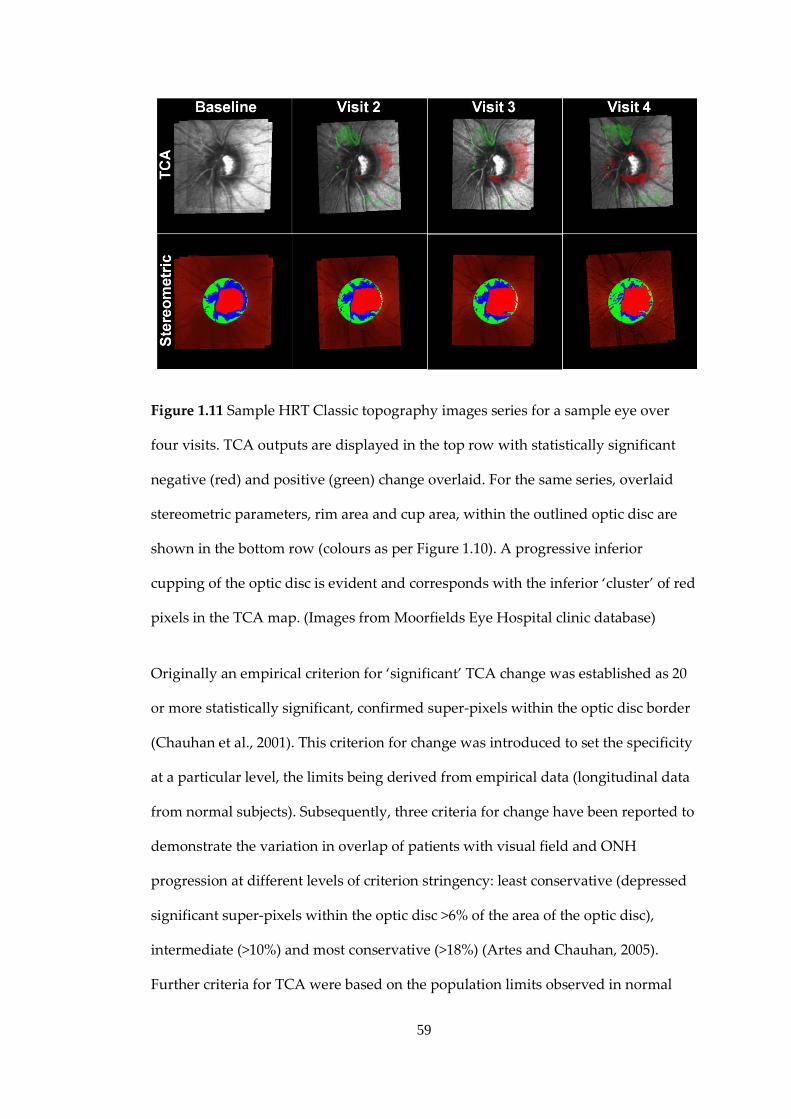
59

Figure 1.11 Sample HRT Classic topography images series for a sample eye over

four visits. TCA outputs are displayed in the top row with statistically significant

negative (red) and positive (green) change overlaid. For the same series, overlaid

stereometric parameters, rim area and cup area, within the outlined optic disc are

shown in the bottom row (colours as per Figure 1.10). A progressive inferior

cupping of the optic disc is evident and corresponds with the inferior ‘cluster’ of red

pixels in the TCA map. (Images from Moorfields Eye Hospital clinic database)

Originally an empirical criterion for ‘significant’ TCA change was established as 20

or more statistically significant, confirmed super-pixels within the optic disc border

(Chauhan et al., 2001). This criterion for change was introduced to set the specificity

at a particular level, the limits being derived from empirical data (longitudinal data

from normal subjects). Subsequently, three criteria for change have been reported to

demonstrate the variation in overlap of patients with visual field and ONH

progression at different levels of criterion stringency: least conservative (depressed

significant super-pixels within the optic disc >6% of the area of the optic disc),

intermediate (>10%) and most conservative (>18%) (Artes and Chauhan, 2005).

Further criteria for TCA were based on the population limits observed in normal

60

subjects (Bowd et al., 2009). In this study, the area (in mm2) of the largest connected

cluster of red super-pixels within the optic disc margin was found to be the best

measure to separate those progressing patients from non-progressing patients at

90%, 95% and 99% specificities. These guidelines reflect that the TCA has no

intrinsic mechanism to account for the multiple comparison problem. The results

are also based only on the comparison of, at most, the four most recent follow-up

images with the baseline image. Thus detecting change is highly dependent on the

quality of the baseline image. In addition because POAG is a slow progressive

disease, there are often many years of follow-up and the TCA essentially ignores

many interim follow-up examinations. Brett and colleagues (Brett et al., 2003)

provide a thorough review of the issues involved in applying statistical techniques

to imaging data including how to account for the multiple comparison problem and

spatial correlation.

Statistical image mapping (SIM) was adapted and applied to HRT imaging of the

ONH by Patterson and colleagues (Patterson et al., 2005) to identify glaucomatous

progression and to address some of the theoretical shortcomings of TCA. This

technique has an established use in analysing 3D images of the brain acquired using

positron emission tomography and magnetic resonance imaging (MRI). In

functional MRI, these techniques are used to process and analyze images to

determine which parts of the brain are activated by different types of physical

sensation, such as sight, sound or movement. A ‘so-called’ statistic image shows a

map of areas of the brain activated by the experiment which can be rendered in

three-dimensions. In particular a non-parametric version of these techniques

(Nichols and Holmes, 2002, Bullmore et al., 1999, Arndt et al., 1996, Holmes et al.,

1996) has been applied to the HRT.

61

In short, SIM proceeds by calculating the trend of topographic change over time, by

performing linear regression on the topographic height for each pixel within the

area of the optic disc; this yields a test statistic summarising the amount of change at

each pixel. The sequence of the images is then reordered (or ‘shuffled’) in time and

the test statistic is recalculated at each pixel. This step is performed a finite number

of times, each time using a unique reordering. At each pixel a distribution of test

statistics is generated and the observed test statistic is then compared to this

distribution, therefore highlighting whether the observed sequence is something

that could have occurred beyond chance. A pixel is flagged as significantly

changing if it falls outside the 95th percentile (a probability value of <0.05). The area

of the largest cluster of contiguous significantly changing pixels in the observed

image series is compared to the distribution of those for the permuted image series.

A global probability value for the entire image series is thus derived from this

distribution position. This value provides a measure of the spatial extent of the

glaucomatous damage which has occurred in the image series and takes account of

the similarity that will exist between topography values of neighbouring pixels. The

method is wholly based on the patient’s own data and the test-retest variability of

the image series, while also correctly accounting for the multiple comparison

problem which occurs when calculating a test statistic at each pixel across an image

space.

1.3.2 Assessing the Performance of Change Detection Algorithms

Apart from theoretical considerations, there is little evidence to suggest that one

method for detecting change is better than another and the clinician is left to

wonder what method for detecting change is best to use.

62

Most research assessing how well these techniques can identify and track

glaucomatous progression with the HRT has focused on examining agreement

between structural and functional measures of progression. In practice, this involves

assessing the diagnostic performance of HRT information in predicting visual field

changes (Miglior et al., 2001, Artes and Chauhan, 2005, Philippin et al., 2006, Saarela

et al., 2010). Studies using visual field changes as a reference standard in this way

can be confounded by dissociating factors between structural and functional

changes (Hudson et al., 2007). As a consequence, the relative proportions of

associated and independent behaviour are not well known and the temporal

sequence of structural and functional glaucomatous progression cannot be well-

defined.

Exploring alternative, and potentially more useful, reference standards against

which the performance of HRT imaging can be assessed may avoid these

confounding factors. Further characterising HRT variability will also help to

determine an optimum approach to detect ONH progression in HRT images. These

investigations will form the main focus of this thesis.

1.4 Objectives

The objectives of this thesis are to assess progression detection algorithms in ONH

data from the CLST. In particular, this thesis aims to:

• Compare the performance of three established competing progression detection

algorithms using the clinical standard for glaucomatous structural damage to

the ONH – expert assessment of optic disc photographs – as the reference

standard

63

• Examine the effects of measurement variability across a range of characteristics

on the statistical performance of some basic univariate statistical techniques to

detect underlying change

• Investigate image quality metrics of HRT images and their relationships to

measurement variability

• Develop and validate a simulation which can reproduce the variability of HRT

data and help to provide a test-bed to evaluate the specificity and sensitivity of

HRT progression detection algorithms

64

2. Glaucomatous Progression in

Series of Stereoscopic

Photographs and Confocal

Scanning Laser Tomograph

Images

Most research on assessing how well glaucomatous progression can be detected

using the HRT has focused on agreement between structural and visual field

measures of progression, or on predicting visual field changes based on HRT

information (Chauhan et al., 2001, Kamal et al., 1999b, Artes and Chauhan, 2005,

Strouthidis et al., 2006, Philippin et al., 2006, Hudson et al., 2007). The fewer

investigations comparing longitudinal HRT and stereophotograph series in humans

(Chauhan et al., 2001, Kourkoutas et al., 2007, Chauhan et al., 2009) have indicated

that agreement between these two structural assessments is moderate with

concordances of 65%, 81%, and 44% to 71% (depending on progression criteria and

expert observers) respectively. Other research in primate experimental glaucoma

showed good agreement between these two imaging methodologies (Ervin et al.,

2002).

The aim of this chapter is to examine change in HRT image series identified by three

automated statistical analytical methods: TCA, SIM, and ordinary least squares

65

(OLS) linear regression of rim area (RALR) against time of follow-up. These changes

are compared to assessments by glaucoma specialists of change in optic disc

stereophotographs from the same eyes in order to determine which method had the

highest concordance with expert assessment of stereophotographs. To control the

sample specificity and sensitivity of HRT change detection analyses, criteria for

change are varied in stringency.

The work in this chapter has formed a paper published in Archives of

Ophthalmology (O'Leary et al., 2010b). It was also presented at the Image

Morphometry and Glaucoma in Europe Meeting, Rotterdam, The Netherlands on

March 12-14, 2008 and the Association for Research in Vision and Ophthalmology

Meeting, Fort Lauderdale on April 27 - May 1, 2008.

66

2.2 Methods

2.2.1 Patients

Data from the Devers Eye Institute Perimetry and Psychophysics In Glaucoma

study are analysed and details of the investigation have been previously published

(Fortune et al., 2007). All of the patients provided voluntary written consent to

participate and to allow their clinical measurements to be securely held for future

data analysis. All of the procedures adhered to the tenets of the Declaration of

Helsinki and were approved by local ethics committee. Participants were recruited

prospectively from the Devers Eye Institute, or other ophthalmic practices in the

Portland, Oregon, metropolitan area. At recruitment, all patients were considered to

have either high-risk OHT or early POAG. All subjects had a history of untreated

IOP of at least 22 mm Hg in both eyes and at least one additional risk factor: a

vertical cup-to-disc ratio of at least 0.6 in at least one eye or an interocular cup-to-

disc ratio asymmetry of at least 0.2; a positive family history of glaucoma; a personal

history of migraine, Raynaud’s syndrome, or vasospasm; African-American

ancestry; or age older than 70 years. All patients met the following criteria for both

eyes: best corrected visual acuity of 20/40 or better and spectacle refraction within

±5.00 dioptre (D) sphere and ±2.00 D cylinder and reliable standard automated

perimetry results with MD better than or equal to -6 dB. Patients were excluded if

they had any other previous or current ocular or neurological disease, previous

ocular surgery (except uncomplicated cataract surgery), or diabetes mellitus

requiring medication. Subjects were treated throughout follow-up at the discretion

of their managing eye care specialists who were sent a copy of study-related test

results yearly.

67

Figure 2.1 Selection criteria applied to stereophotograph and HRT progression

study and the resulting sample sizes.

68

2.2.2 Selection Criteria for Study

Data from an initial dataset of both eyes of 168 patients (336 eyes) with follow-up of

at least 4 years (median=6.1 years) were evaluated. Figure 2.1 illustrates the selection

criteria from this initial dataset with the numbers of patients and eyes in the study

as selection criteria are applied.

2.2.3 Stereo Optic Disc Photography and Grading

Photographs were obtained annually for all of the patients using a simultaneous

stereoscopic camera (3-Dx; Nidek Co., Ltd., Gamagori, Japan) after maximum pupil

dilation. For each eye, the photographs obtained at baseline and at the most recent

follow-up visit were randomly assigned to be labelled as A or B, to mask the

temporal order. All other information about the eye and the patient was masked

from the graders, including the appearance of the fellow eye. Two fellowship-

trained glaucoma specialists independently viewed the baseline and final follow-up

photographs sequentially using a Stereo Viewer II (Asahi-Pentax, Tokyo, Japan) and

graded them as “changing” or “stable”, indicating which photograph showed worse

damage (A or B). If there was change, the type of change was recorded, as one or

more of the following: increased neuroretinal rim narrowing, increased excavation,

new or increased retinal nerve fibre layer defect or new notching. The location of

change was recorded in 90 degree sectors (0 -̊90˚, 90˚-180˚, 180˚-270˚ and 270˚-360˚).

Quality assessments of each image pair were recorded separately for clarity and for

stereopsis as ‘excellent, ‘adequate’ or ‘unacceptable’.

The reviewers mediated disagreements by re-examining the photographs together

to reach consensus; any continuing disagreements between these two graders were

adjudicated by a third masked expert. Change identified in the correct temporal

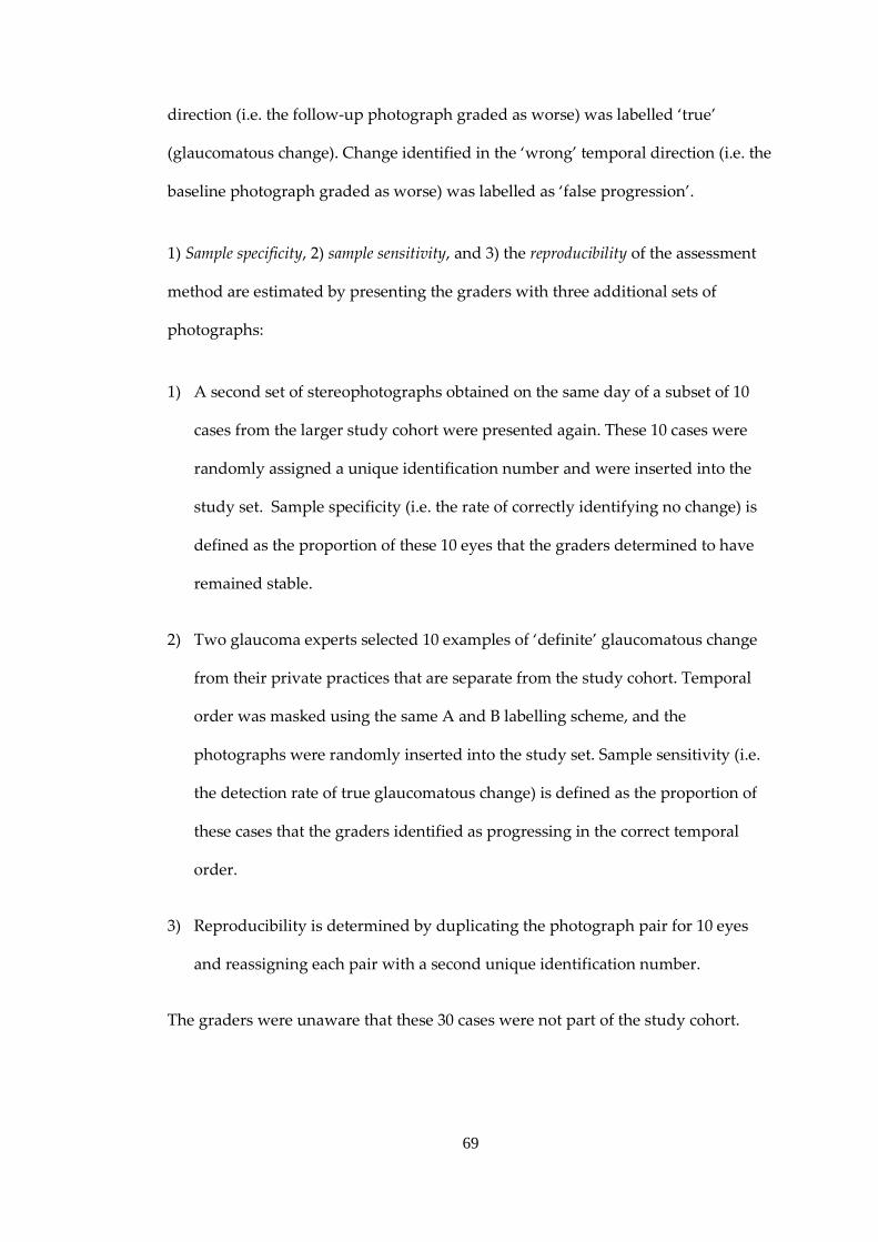
69

direction (i.e. the follow-up photograph graded as worse) was labelled ‘true’

(glaucomatous change). Change identified in the ‘wrong’ temporal direction (i.e. the

baseline photograph graded as worse) was labelled as ‘false progression’.

1) Sample specificity, 2) sample sensitivity, and 3) the reproducibility of the assessment

method are estimated by presenting the graders with three additional sets of

photographs:

1) A second set of stereophotographs obtained on the same day of a subset of 10

cases from the larger study cohort were presented again. These 10 cases were

randomly assigned a unique identification number and were inserted into the

study set. Sample specificity (i.e. the rate of correctly identifying no change) is

defined as the proportion of these 10 eyes that the graders determined to have

remained stable.

2) Two glaucoma experts selected 10 examples of ‘definite’ glaucomatous change

from their private practices that are separate from the study cohort. Temporal

order was masked using the same A and B labelling scheme, and the

photographs were randomly inserted into the study set. Sample sensitivity (i.e.

the detection rate of true glaucomatous change) is defined as the proportion of

these cases that the graders identified as progressing in the correct temporal

order.

3) Reproducibility is determined by duplicating the photograph pair for 10 eyes

and reassigning each pair with a second unique identification number.

The graders were unaware that these 30 cases were not part of the study cohort.

70

2.2.4 Confocal Scanning Laser Tomography

The CSLT images were obtained using the HRT Classic. Several single topographies

per examination were acquired and the three best-quality images (by subjective

assessment) were combined to create a mean topography for each eye. An

experienced operator outlined the optic disc margin. Images were analysed using

the latest available software (version 1.6.1.0) but are not imported to HRT III

software. The manual land-marking facility was used to correct obvious failures of

the automatic alignment algorithm to adequately register images across time.

2.2.5 Statistic Image Mapping

SIM (as discussed in Chapter 1) is applied to topographic image series in this study.

Its full methodological details can be found elsewhere (Patterson et al., 2005). Unlike

the TCA, SIM is not integrated into the HRT software as a tool for progression

analysis. The SIM algorithm was reproduced entirely in MATLAB (R2009a, The

MathWorks Inc, Natick, Massachusetts) utilising an image-wise linear regression for

each re-ordered image series which was programmed to take advantage of the

platform’s more efficient matrix operations. A map of significant change is

produced at each final follow-up examination along with a significance value for the

largest connected cluster of significantly negatively changing pixels. For an image

series of length 10 examinations processing time is approximately 6 minutes on a

2.66 GHz dual core processor comparable to the reported 3 minutes of the original

algorithm coded in the C computing language (Patterson et al., 2005).

71

2.2.6 Topographic Change Analysis

TCA was performed on the data as per the description in Chapter 1. This is

implemented as follow: using the super-pixel change probability maps and mean

difference from baseline maps, exported from the HRT software, a significant

change map is constructed for each follow-up examination. This is done by

identifying super-pixel locations with significant decrease in the retinal height from

the baseline examination (i.e., the locations with negative height change in the mean

difference image and change probability < 0.05). Change across time is confirmed by

comparing the most recent follow-up examination findings with those of the

previous 2 examinations producing a final TCA map.

2.2.7 Linear Regression of Rim Area

As detailed in Chapter 1 of this thesis RA has been shown to give information which

is clinically meaningful and also more reproducible than the other stereometric

parameters from the HRT. Consequently is likely to be a better candidate among

these for detecting and tracking glaucomatous structural changes. RA analysis for

this study is trend-based. Global RA and RA for the six pre-defined sectors are

analysed across time using OLS linear regression and p-values obtained for the null-

hypothesis that the trend of the linear fit is <0mm2 per annum. The fixed 320µm

reference plane is used for all RA calculations (Burk et al., 2000) because it has been

shown to improve the repeatability of RA measurements (Strouthidis et al., 2005a,

Breusegem et al.).

72

2.2.8 Analysis: Measures of Change and Sliding Scale

For SIM, the measure of change is the probability value of the largest cluster of

‘active’ (red) pixels. In the TCA, the measure of change is the area of largest cluster

of red super-pixels as a percentage of disc area. In the case of RA, the measure of

change is the lowest p-value (most significant) obtained by LR of the 7 (global and 6

sector) RA linear trends. Using expert-assessed stereophotographs as the reference

standard, the aim is to vary the criteria for change for each method of HRT change

analysis and compare proportions identified as changing. Thus, receiver operating

characteristic (ROC) curves are generated to measure the diagnostic precision of

each HRT change-analysis method in predicting glaucomatous optic disc changes

assessed on stereophotographs. ROC curves are discussed further in Chapter 3.

Agreement between HRT methods and stereophotograph change, at equal rates of

glaucomatous progression classification, is examined and illustrated using area

proportional Venn diagrams. This entailed fixing discriminant criteria to classify the

same number of eyes as changing in HRT analyses as in the stereophotograph

assessment. Analysis was carried out in MATLAB (R2009a, The MathWorks Inc,

Natick, Massachusetts)

73

2.4 Results

Ninety-one eyes of 56 patients from the original 336 eyes of 168 patients met the

chronological and quality criteria (Figure 2.1). The proportion of glaucomatous and

OHT patients was 87.5% and 12.5% respectively. Measurements from 7 annual,

mean HRT scans (composed of 3 single HRT scans) for each eye in this study are

used for analysis. Mean patient age at baseline was 56 years (range 35-82 years) and

the male-female ratio was 52:48. The racial mix was as follows: 54 (96%) white; 1

Hispanic and 1 American Indian.

In the patient dataset, 33 eyes (36%) were assessed as exhibiting glaucomatous

change using the stereophotograph reference standard. In 47 out of 91 instances

(52%) the assessment required adjudication by the third grader (Table 2.1).

The mean interval between baseline stereophotograph and baseline HRT scan

acquisition was 8 days and the mean interval between follow-up stereophotograph

and final follow-up HRT scan acquisition was 11 days.

Of the same-day stereophotograph set, 2 of 10 eyes were judged to be changing by

graders, giving sample specificity of 80% (95% CI, 44%-98%). Of the definite

glaucomatous change set, 8 of 10 eyes were judged to be changing. Of the repeated

set, 2 of 10 stereophotograph pairs resulted in different assessments on repeated

presentation. Thus sample sensitivity and reproducibility are both estimated to be

80% (95% CI, 44-98%).

Figure 2.2 shows the ROC curves for TCA, SIM and RALR. Areas under the ROC

curves (95% CIs) are as follows: 0.61 (0.56 - 0.66) for TCA; 0.62 (0.57 – 0.67) for SIM;

and 0.66 (0.61 – 0.71) for RALR. Using the method of Hanley and McNeil (Hanley

74

and McNeil, 1983b) to compare areas under two ROC curves resulted in p=0.79, 0.26

and 0.24 for pair-wise comparisons of TCA/SIM, TCA/RALR and SIM/RALR

respectively. At a fixed specificity of 90% for all three methods, sensitivities are 25%

for TCA, 27% for SIM and 40% for RALR, respectively.

Table 2.1: The summary of stereophotograph assessment of progression in the

study with the proportion of assessments reached by consensus and the proportion

requiring adjudication.

Progression

Yes No Total

Mod

e of

D

ecis

ion Consensus 11 (12%) 33 (36%) 44 (48%)

Adjudication 22 (24%) 25 (27%) 47 (52%)

Total 33 (36%) 58 (64%) 91 (100%)

75

Figure 2.2 ROC curves for HRT progression algorithms using stereophotograph-

assessed glaucomatous change as the reference standard for TCA, SIM and RALR.

Areas under the ROC curves are 0.62 for SIM, 0.61 for TCA and 0.66 for RALR.

Figure 2.3 shows the agreement of TCA, SIM and RALR identified change with

stereophotograph change, after rates of identified progression are matched to those

of the stereophotograph assessment (36%). Concordances are 0.54 for TCA, 0.65 for

SIM and 0.67 for RALR and associated Cohen’s 𝜅 values are 0.05, 0.23 and 0.30

respectively. Figure 2.4 shows the agreement among the HRT change-detection

methods at equal rates of identified change (36%). This reveals concordances among

the HRT change-detection methods to be 60% and pair-wise concordances of

between 71% - 76%.

76


SIM and RALR with stereophotograph assessment. Equal rates of identified

progression mean that the circles in each diagram are equal in area.

77


SIM and ordinary RALR with each other in determining glaucomatous progression.

Equal rates of identified progression mean that the circles are equal in area.

Figures 2.5-2.8 show 4 cases to illustrate different levels of agreement between HRT

analyses and stereophotograph assessment when criteria for progression are fixed

for equal classification rates. The stereophotograph decisions were reached by

consensus in case 1 and case 4 but required adjudication in cases 2 and 3.

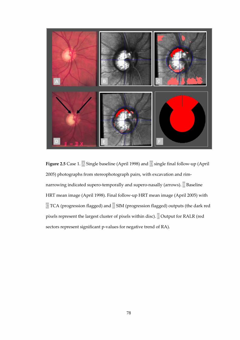
78

Figure 2.5 Case 1. A Single baseline (April 1998) and D single final follow-up (April

2005) photographs from stereophotograph pairs, with excavation and rim-

narrowing indicated supero-temporally and supero-nasally (arrows). B Baseline

HRT mean image (April 1998). Final follow-up HRT mean image (April 2005) with

C TCA (progression flagged) and E SIM (progression flagged) outputs (the dark red

pixels represent the largest cluster of pixels within disc). F Output for RALR (red

sectors represent significant p-values for negative trend of RA).

79

Figure 2.6 Case 2. A Single baseline (August 1998) and D single final follow-up


infero-temporally (arrow). B Baseline HRT mean image (August 1998). Final follow-

up HRT mean image (August 2005) with TCA C (no progression flagged) and SIM E

(no progression flagged) outputs (dark red pixels represent largest cluster of pixels

within disc). F Output for RALR at (red sector and centre represent significant p-

value for negative trend of RA).

80

Figure 2.7 Case 3. A Single baseline (October 1998) and D single final follow-up


infero-temporally (arrow). B Baseline HRT mean image (October 1998). Final follow-

up HRT mean image (August 2005) with TCA C (no progression flagged) and SIM E

(no progression flagged) outputs (dark red pixels represent largest cluster of pixels

within disc). F Output for RALR (green centre represents no significant p-values for

negative trend of RA).

81

Figure 2.8 Case 4. A Single baseline (July 1998) and D single final follow-up (July

2005) photographs from stereophotograph pairs with no observed change. B

Baseline HRT mean image (July 1998). Final follow-up HRT mean image (July 2005)

with TCA C (progression flagged) and SIM E (progression flagged) outputs (dark

red pixels represent largest cluster of pixels within disc). F Output for RALR (red

sector and centre represent significant p-value for negative trend of RA).

82

2.5 Discussion

The CLST, as typified by the HRT, has been shown to give a repeatable measure of

optic disc structure (Dreher et al., 1991, Cioffi et al., 1993, Chauhan et al., 1994). The

HRT does reasonably well in distinguishing glaucomatous eyes from healthy eyes

(Mikelberg et al., 1995, Asawaphureekorn et al., 1996, Bathija et al., 1998, Wollstein

et al., 1998, Swindale et al., 2000, Zangwill et al., 2001, Coops et al., 2006). The real

promise of the technology may be in offering a reliable method for tracking

structural change, potentially providing useful clinical management information

about disease stability. A method for quantifying change is required to realise this

potential and there has been much research activity in developing an appropriate

technique (Chauhan et al., 2001, Tan and Hitchings, 2003, Patterson et al., 2005,

Strouthidis et al., 2006, Fayers et al., 2007) but there is little evidence to suggest that

one method is better than another.

Studies using functional progression (visual field deterioration) (Girkin, 2004b,

Sample et al., 2002, Artes and Chauhan, 2005, Strouthidis et al., 2006) are

confounded by aspects of the relationship between structural and functional

changes. The relative proportions of associated and independent behaviour are not

well-known and the temporal sequence of structural and functional glaucomatous

change is not well-defined. Because change identified by structure and function do

not seem closely related, it may be more likely that progression identified by

glaucoma experts from optic disc stereophotographs would provide a better

reference standard against which to assess the performance of another structural

measurement for progression (CSLT images).

83

This study is one of few examining agreement of HRT change analyses with expert

assessed stereophotographs (Chauhan et al., 2001, Ervin et al., 2002, Chauhan et al.,

2009, Kourkoutas et al., 2007). A variety of statistical methods are considered for

detecting change in HRT images and the stringency of the criteria for HRT change

was varied to give a measure of sample sensitivity across the full range of sample

specificity. This study took advantage of data from a carefully collected prospective

longitudinal study across a relatively long period, and strict image quality criteria

were applied. Previous research (Morgan et al., 2005) has shown better between-

grader agreement and better reproducibility from stereophotographs than from

monoscopic photographs when discriminating between glaucomatous and healthy

discs. The estimate of reproducibility for expert assessed progression in

stereophotographs in this study, at 80%, is comparable with that of previous studies

that have obtained 𝜅 values of 0.62-0.89 (Parrish et al., 2005) and 0.80-1.00 (The

European Glaucoma Prevention Study Group, 2003) for within-observer

reproducibility.

The ROC analysis suggests that, when using stereophotograph assessment as the

reference standard, automated HRT methods have only moderate precision to

predict change. The ROC curves revealed poor sample sensitivities for clinically

relevant regions of high sample specificity. At equal rates of classification, poor

agreement is found between the expert-assessment of stereophotographs and the

HRT analyses. Both stereophotographs and HRT images are assumed to give an

accurate and repeatable measure of the structure of the optic disc but the false-

positive and false-negative rates of both the reference standard and the HRT

methods may largely explain this poor agreement. This is illustrated in cases 1-4

(Figures 2.5-2.8). The false positive rate of photograph grading from this study

(estimated to be 20%) is a major factor. This rate falls within the range of previous

84

studies (Ervin et al., 2002, Chauhan et al., 2009) (ranges of 0% - 50% and 5% - 77%

respectively depending on stringency of progression criteria and observers).

Furthermore, grader agreement, even between ‘experts’, in other tasks, such as

separating healthy and unhealthy optic discs, (Reus et al., 2007) or assessing

progression events in series of optic disc stereophotographs (Jampel et al., 2009,

Chauhan et al., 2009) and visual fields (Viswanathan et al., 2003) is not good.

Owing to the nature of this dataset (generally early glaucoma) there is likely to be a

wide range in the magnitude of changes and agreement may be much worse when

changes are of small magnitude, partly evidenced by the 52% of stereophotograph

assessments that required adjudication by a third expert.

Further reasons for the difference may be that features sometimes implicitly

attributed to glaucomatous change in stereophotographs (e.g. colour changes) may

not be apparent in HRT images which are simply estimates of the topographic

height of the optic disc surface and surrounding areas. Other contributing factors

are that certain optic disc configurations (such as hypoplastic and tilted discs) may

present greater difficulty for either HRT analysis (image registration, contour line

fitting and RA calculation) or stereophotograph assessment.

Concordance among all three statistical methods for detecting HRT change is 60%

and pair-wise concordance are 71% to 76%. It is not surprising that agreement

among HRT analyses is better than is agreement between stereophotograph

assessment and HRT analyses. Differing statistical methods such as those used in

this study will never have perfect concordance even on the same data. However the

level of disagreement between HRT analysis methods is probably amplified by the

low stringency of the change criteria (fixed to identify equivalent 36% -

proportions), and the related (likely) high false-positive rate. These criteria are less

85

stringent than those used in previous studies (Chauhan et al., 2001, Patterson et al.,

2005).

The results of this study expose the limitation of using grader-assessed

stereophotographs alone as a reference standard for structural glaucomatous

progression. Future studies to assess the effectiveness of HRT change analysis

methods may require a more innovative approach to establishing a reference

standard. Using an accumulation of information from a variety of measurements

(visual field, IOP and optic disc) and presenting this as a continuous scale for

evidence of change might be useful (Artes and Chauhan, 2005). Another approach

might be to simulate series of images with known properties, using a virtual

platform in which the CSLT image formation process is simulated computationally

from a baseline scan. Automated analysis of the reconstructed optic disc from

stereophotographs may also be useful (Xu et al., 2008). Imaging devices, such as

spectral domain OCT, which may give surrogate measurements closer to what is

really required to detect real glaucomatous change, may also help refine reference

standards for progression.

Though this is outside the scope of this study, it is worth remembering that

progression detection is not necessarily a binary classification between changing

and not changing. There are a small proportion of patients who are likely to suffer

large glaucomatous damage in a short space of time while the typical patient

experiences slow changes over a long period of time with a continuum in between.

This continuum has been observed in visual field data of untreated patients (Heijl et

al., 2009). So it is important to distinguish this complementary approach and

address the issue of reporting the best estimates of optic disc changes along with the

statistical confidence in these.

86

There are other limitations to this study. Varying criteria for progression in

stereophotograph assessment would have been useful in determining various

diagnostic strengths of the HRT analyses (Chauhan et al., 2009) but may also have

led to even less agreement between graders. The setting of a cut-off criterion to

determine progression is not trivial: because the true specificity of a criterion cannot

be known, setting the cut-off value to result in equal rates of progression provides

an opportunity to compare the agreement between the HRT change detection

methods when the ‘hit-rate’ is the same. Times to progression were not examined, in

part due to stereophotographs being assessed only at baseline and final follow-up.

Therefore there are no estimates to report as to which HRT analyses detected change

earliest, although one could question the value of such analyses when agreement

between methods is poor. The number of eyes in the definite glaucomatous change

stereophotograph set and the same-day (no glaucomatous change) set are low,

resulting in large CIs for the estimates of sample specificity and sensitivity for the

expert-assessed change. However, as already discussed, these estimates are similar

to those of previous studies. Because only ‘depressed’ change is examined in HRT

topographies, glaucomatous change resulting in elevation of the optic disc surface

(if it occurs), would have been overlooked. However, given the nature of glaucoma,

this approach seems reasonable given that an elevation may be more indicative of

measurement noise or morphological change independent of glaucoma than a

depression and may have resulted in a higher rate of falsely detected glaucomatous

change. Moreover, the ability to accurately detect changes, or lack of changes, in

HRT longitudinal image series will depend enormously on the ability of the

software to register the images appropriately and thus these results are limited by

the constraint of the HRT alignment algorithm. Only HRT Classic (10° x 10°) images

were available in the study which although wide enough to contain the optic disc in

87

all cases, have less available features for registration than HRT II (15° x 15°)

resulting in poorer alignment in the latest HRT software (Bergin et al., 2008). Also

HRT Classic topography series unlike HRT II series, are not corrected for parabolic

error between mean topographies caused by axial movement of the eye between

exams (Balasubramanian et al., 2011), potentially leading to further topographic

variability.

A separate analysis of glaucomatous and OHT patients may have revealed

differences in the rates of change in stereophotograph assessments and HRT

algorithms but the number of OHT patients was so low as to limit the reliability and

utility of any inferences from this comparison. Finally the resulting proportion eyes

progressing by stereophotograph assessment should be used with caution when

extrapolating to groups of non-white patients and groups with more established or

later stage glaucoma.

In conclusion, this study revealed poor agreement between progression detection

using a variety of HRT statistical methods and expert-assessed stereophotographs of

the optic disc. Using stereophotograph-assessed change as the reference standard

does not help determine which HRT change algorithm best identifies glaucomatous

change in this group of patients with high risk OHT and those with early glaucoma.

This does not imply that stereophotographs are not integral to the assessment of

glaucomatous change. Indeed they are a clinically well-accepted standard that have

been used in major clinical trials. However, the diagnostic precision associated with

observer stereophotograph-assessed change precludes it from being a stand-alone

benchmark by which to evaluate alternative change detection tools. The practical

benefits of being able to observe change using automated or semi-automated digital

image analysis, and other recent evidence, (Chauhan et al., 2009) suggest that it is an

88

important tool for assessing disease progression, especially if a statistical method for

best detecting the change can be established. The extent to which these algorithms

measure real ONH changes across time in HRT image series and their related

stereometric parameters will need to be established in other ways and this will be

addressed in the following chapters.

89

3. Trend Detection in Series of

Univariate Measurements

It is well established that POAG is a slow progressive disease which requires

continuous management by the clinician. This means that, once diagnosed, POAG

patients will need clinical follow-up examinations for the rest of their lives. The

advantage of an approach for measuring change as a trend will be that it can

incorporate information from the often long series of follow-up measurements more

readily than an event analysis and give a clinician a better insight on the success (or

failure) of certain treatments with a particular patient. The estimation of trends in

metrics such as global RA and mean RNFL thickness has an important role as a

summary measure by which to quantify optic disc changes measured by imaging.

RA and RNFL are surrogate measures of axonal health and trends in these are

relevant in that a general decrease over time can serve as a measure of

glaucomatous axonal loss. They also lend themselves readily to clinical

interpretation: change in an area can be easier to appreciate visually and interpret

than a change in a topographic height. When attempting to detect true

glaucomatous structural change it is necessary to firstly identify statistically

significant changes before determining if the change represents an amount of loss to

warrant a change in treatment or further or more thorough examinations. A

statistical model which describes just one variable is known as a univariate model and

it is the purpose of this chapter to examine univariate models for detecting trends in

an individual stereometric parameter (in this case RA) with equal application to

detecting change in other stereometric parameters and much more localised

measures such as in the individual pixels or super-pixels of topographic images.

90

Statistical models of univariate trends in glaucoma have mostly taken the simplest

of forms. Linear models of change with simple (but strong) assumptions about the

measurement noise are frequently used in modelling longitudinal series of both

localised and global visual field (Hitchings et al., 1994, Fitzke et al., 1996,

Viswanathan et al., 1997, Gardiner and Crabb, 2002a, Heijl et al., 2009) and

structural measures (Strouthidis et al., 2006, See et al., 2009). The linear model

requires fewer parameters than more complicated models and crucially provides an

easy to understand average linear trend across time at any point in time which is

equivalent to the average change per unit time over the whole follow-up. Because of

the strong assumptions it makes, it is known as a parametric model. Another model

of change, by ranking measurements, has been used before to establish the evidence

of change in sectoral RA measurements (Artes and Chauhan, 2005). This type of

easily understood model makes very few assumptions of the data – and is known as

a non-parametric model. As a result, this type of method can be more appropriately

applied to a wider range of data series where change may not follow a linear trend

and it is potentially more robust to outliers. This rank-based approach does not

however provide a measure of change but merely indicate if there is evidence for a

trend occurring over time. Other approaches such as those assuming a linear model

but drawing statistical inferences by non-parametric means can be classified as semi-

parametric methods such as that used in SIM pixel-wise analysis for detecting

significantly changing topographic locations over time (Patterson et al., 2005). Along

with the strength of the underlying trend, the measurement variability of any data,

will govern how well this trend can be detected by any statistical technique.

The variability of ONH imaging data is frequently reported but rarely characterised

beyond the most summary of descriptors such as the standard deviation or

coefficient of variation. These measures are used to helpfully distinguish if one area

91

of the ONH has greater measurement variability than another (Tan et al., 2003,

Strouthidis et al., 2005b) or if one device has greater measurement variability than

another (Kim et al., 2009). Though it is useful for these comparisons the standard

deviation is sufficient only in characterising variability from a normal distribution.

Other characteristics of measurement variability such as the skewedness (the

tendency of a distribution to be smeared in one particular direction) or the kurtosis

(the tendency of a distribution to have heavier tails) of the measurement variability,

and ideally an empirical fitting of different distributions to measurement variability

distributions are desirable. There is a notable exception to this in analysis of HRT

RA data (Owen et al., 2006). This analysis by Owen and colleagues has

demonstrated that both the test-retest and longitudinal measurement variability of

RA are non-normally distributed.

Furthermore, in many fields, the dependence of the variability of a measurement on

the underlying value of the measurement is not always uniform. This phenomenon

is termed heteroscedasticity and the case where variability remains uniform is called

homoscedasticity. This is especially relevant for modelling change as by definition the

measurement will change over time. It is well known that the variability of visual

field sensitivity is associated with loss of sensitivity (Henson et al., 1999, Spry et al.,

2001). No theory that test-retest or longitudinal RA variability change with RA itself

has been established. There is evidence both for (Tan et al., 2003, Leung et al., 2008,

Lin et al., 2009) and against (Strouthidis et al., 2005b, Jampel et al., 2006) stage of

disease being related to same-eye variability of HRT topographic and morphological

measures though it is likely that these latter studies did not have a sufficient range

of RA to show any relationship. For those studies reporting changes in RA

variability with disease stage, an increase has been consistently shown for more

92

advanced disease stage. Thus it is worthwhile investigating the potential effects of

changes in RA variability over time.

Another potentially difficult factor for any statistical change detection technique to

address is that measurements in a series (or the measurement errors) may have

some relationship to each other. This relationship of serial measurements with each

other is known as autocorrelation. This can be periodic as in the case of the circadian

changes in IOP (Hughes et al., 2003) and is often seen on a longer timescale in the

form of seasonal effects (Giuffre et al., 1995, Wu and Leske, 1997). No studies have

systematically investigated any periodic changes in ONH data from the HRT (or

any other devices) beyond the short time-scale of the cardiac cycle (Chauhan and

McCormick, 1995). A single case study has shown an large variation in RA of a

patient with a large circadian IOP amplitude (Lee et al., 1999) and another study has

shown that induced acute IOP increases result in increased optic disc diameters

(Poostchi et al., 2010) which may affect RA .

One way to investigate the false positive detection rate from statistical methods is to

use real data in which any detection of statistically significant changes or trends will

be due to measurement noise alone. A ‘stable’ dataset in which it is highly unlikely

for any measured change to be associated with glaucomatous pathology; in

particular, a series of many repeated measurements acquired over a short period of

time can be useful for this. This circumvents the need for an external gold standard

of stability in serial ONH measurements. The use of a Monte Carlo simulation

(Metropolis and Ulam, 1949) has, with the advent of increased computing power,

offered applied statisticians an accurate tool to compare and contrast statistical

methods where analytical solutions are not easily available. This approach is taken

to assess the ability of statistical algorithms to detect underlying trends buried in

93

noisy data without confounding effects from an uncertain reference standard of

change. In a simulation setting, measurement variability can be designed to be

representative of that of real data with the further advantage that it is also possible

to simulate series where an underlying trend is present and known in advance.

Given that we know so little about the trends governing RA change over time and

the measurement noise characteristics, it seems wise to experiment with a range of

‘scenarios’ in which different combinations of measurement variability and trends

are used to assess the performance of change detection techniques of interest.

The aim of this chapter is to assess the performances of different parametric, semi-

parametric and non-parametric univariate statistical techniques for detecting trends

using both short-term ‘stable’ series and simulated series. Simulation allowed the

design of multiple ‘scenarios’ of series with different measurement variability and

magnitudes of underlying change (known by design) which approximate to real

data.

94

3.1 Trend Detection Techniques

In assessing a series of univariate measures over time, the clinician, clinical scientist

or computer algorithm is presented with a series of 𝑛 measurements (in the case of

this analysis, RA measurements) 𝑦𝑖 = (𝑦1,𝑦2 … , 𝑦𝑛) at corresponding time

points 𝑡𝑖 = (𝑡1, 𝑡2 … , 𝑡𝑛). To detect an underlying trend in this data involves

devising a model of change over time, fitting this model to the data and testing that

the fitted model has a significant trend with a hypothesis test.

One of the simplest approaches to this might be to assume a linear trend model

along with other assumptions (below) and to perform an OLS linear regression. In

general terms, OLS regression is an approach to quantifying the relationship

between a scalar variable 𝑦 to one or more predictor variables denoted 𝑋 by

optimally fitting the observed variables to an assumed model giving “best-fit”

parameters for this model. In OLS linear regression, a linear model and its estimated

parameters are used to estimate this relationship. In the case of trend analysis the

OLS linear regression approach would be to model time as a predictor variable and

its linear relationship with whatever measurements are being observed over time.

The principal assumptions of OLS are that there are no errors in the predictor

variable (time) with the following additional assumptions (Salkind and Rasmussen,

2007):

1. Measurement errors about each point are sampled from a normal distribution

with a mean of zero (normally distributed)

2. Distributions from which measurement errors are sampled do not change across

the predictor variable (identically distributed/homoscedastic)

95

3. Successive measurement errors are independently sampled (independent/non-

autocorrelated)

These assumptions are strong and it is likely that scenarios exist in serial

measurement of clinical data such as RA measurements where these are violated -

these have been discussed in the introduction to this chapter. Under assumption of

the normality of the error terms, the estimator of the slope coefficient will itself be

normally distributed (Salkind and Rasmussen, 2007). As a result, the hypothesis-test

regarding the significance of the trend measured by OLS linear regression (after an

appropriate adjustment for the measurement noise) can be inferred from a

theoretical student’s t-distribution. For this reason OLS linear regression trend

detection is referred to as a parametric method. Other means of modelling trends

(see (c) below) and other means of performing hypothesis tests in a non-parametric

fashion are readily implemented and easily understood for trend detection and will

be used in the analysis of this chapter along with OLS linear regression.

A permutation test is a hypothesis test which infers the significance of a test-statistic

from distribution of test-statistics under reordering of measurements. Evolving from

the work of Pitman in the 1930s (Pitman, 1937), these tests have come to form a

subset of non-parametric statistical methods best used when it is unknown how this

a test-statistic is distributed (Good, 2005). For a trend analysis, it involves permuting

or reordering the time labels in a series of observed measurements, calculating a

test-statistic such as a linear regression slope or Spearman’s 𝜌 and replicating this to

cover all possible unique reorderings. The null hypothesis is simple: “there is no

underlying trend in the observed series” and if so then the trend test-statistic in the

observed series will not be different to the permutation distribution. The position of

the observed test-statistic in the permutation distribution will govern its inferred

statistical significance. The exchangeability of a sequence ensures the correct

96

inferences are made from permutation testing (Good, 2005). The advantage of this

approach is in removing the assumption about the underlying distribution of the

test-statistic by replacing it with the permutation distribution thus making it more

robust in datasets which do not adhere to parametric assumptions. For practical

purposes, the number of reorderings is limited in this analysis of this chapter at a

maximum of 1000.

In this analysis the following particular three trend detection techniques are chosen

and classified as (a) fully parametric, (b) semi-parametric and (c) non-parametric

techniques:

(a) OLS T-DIST: OLS regression with significance of slope inferred from the position

of the parametric test statistic in the student’s t-distribution. Linear regression

attempts to describe the association between two independent variables and can

serve as a form of trend analysis when one of the variables is time. (This is the same

technique used in Chapter 2 for RA analysis - labelled RALR.).

(b) OLS P-DIST: An OLS linear regression method (parametric) with the

significance of the observed slope inferred non-parametrically from permutation

distribution of slopes (OLS SL P-DIST). This method has been used before to detect

the significance of observed change in series of images at a pixel level to identify

glaucomatous progression (Patterson et al., 2005) and also applied to the area of

functional neuro-imaging (Holmes et al., 1996). Appendix A provides a derivation

for the monotonic relationship of the slope and the slope/standard error test-statistic

distributions within a permutation test used by Patterson and colleagues. This

simply means that the standard error of each permuted slope estimate need not be

calculated: the slope alone can be permuted to obtain the same rank (position) in a

permuted distribution as the slope-standard error ratio. By parametrically fitting the

97

underlying linear trend by OLS, and as it does not rely in a significance estimate

from the Student’s t-distribution, this method can be termed semi-parametric.

(c) RHO P-DIST: Spearman’s rank correlation coefficient 𝜌 is a non-parametric

measure of the association between two variables – essentially quantifying how well

the relationship between the two variables can be described by a monotonic

function. This is performed by comparing the rankings of each variable in pairs. By

letting one of these variables be time, this becomes a measure of trend of the other

variable. Spearman’s 𝜌 is the test statistic for underlying trend. For a given sample

of 𝑛 paired data (𝑡1,𝑦1),...., (𝑡𝑛,𝑦𝑛), let 𝑅𝑖 = rank(𝑡𝑖) and 𝑆𝑖 = rank(𝑦𝑖) this

is defined by:

𝜌 =∑ (𝑅𝑖 − 𝑅�)(𝑆𝑖 − 𝑆̅)𝑛𝑖=1

�∑ (𝑅𝑖 − 𝑅�)∑ (𝑆𝑖 − 𝑆̅)𝑛𝑖=1

𝑛𝑖=1

where 𝑅� = 𝑆̅ = (𝑛+1)2

is the average rank. If some values of 𝑅 or 𝑆 are tied, these

values are simply assigned the average of the ranks to which they would have been

assigned. A permutation test is used to derive the significance of the test statistic

from the observed series. Rank based methods such as this have been applied to

detecting underlying trends in areas such as environmental and hydrological

sciences and an review of these and other trend detection techniques can be found

in Hipel and MacLeod (Hipel and McLeod, 1994).

For all methods, hypothesis tests are one-sided i.e. testing if trends are significantly

less than zero. As discussed in Chapter 2, given that an underlying negative trend of

RA damage is expected to be indicative of an optic disc with progressive

glaucomatous, the investigation of statistically significant positive trends in RA

series seems unnecessary.

98

3.2 Data

Both real and simulated datasets of ‘stable’ RA series are used to assess the

performance of change detection techniques. Without knowledge of the underlying

signal in many real datasets, simulation will serve to generate data with known

trends of measured RA change over time. Underlying trends are simulated

according to estimates in a previous study examining OHT patients developing

significant glaucomatous damage (Owen et al., 2006). These trends are assumed to

be characteristic of those found in progressing glaucoma patients though differences

in the type and stage of glaucoma may well differ.

3.2.1 Real Data

Seventy-four eyes of 74 subjects recruited from the OHT clinic at Moorfields Eye

Hospital were included in an HRT test-retest study detailed elsewhere (Strouthidis

et al., 2005b). In short, 43 eyes with OHT and 31 with POAG were selected. The

subjects had no previous history of intraocular surgery and had all experienced

ONH imaging using the HRT. This study adhered to the tenets of the Declaration of

Helsinki and had local ethics committee approval and the subjects’ informed

consent. OHT is defined as IOP greater than 21 mmHg on two or more occasions

and a baseline Humphrey 24–2 full threshold AGIS score of 0. POAG is defined as a

consistent AGIS visual field score greater than 0, and a pre-treatment IOP greater

than 21 mmHg on two or more occasions. Each eye was selected on the basis that it

had a refractive error less than 12 dioptres of spherical power and no history of

previous intraocular surgery. In subjects with lens opacity, the eye with the greater

degree of opacity was preferentially selected although the presence of lens opacity

itself was not a criterion for subject selection. HRT Classic images (10° scan width)

99

and HRT II images (15° scan width) were acquired across two visits within 6 weeks.

A total of five HRT Classic mean topographies and five HRT II mean topographies

were generated for each eye. Three HRT single topographies were used to generate

a mean topography for both HRT Classic and HRT II data. After satisfying the

device checks of minimal eye movement, acceptable focus and illumination during

acquisition there were no criteria placed on image quality. Thus the ranges of media

opacity and image quality are large. The mean age of patients at baseline was 68.2

years (standard deviation 10.2 years) and the male:female ratio was 41:33.

These data are separated into those with HRT Classic data only and those with HRT

II data only. This minimises any potential artefact which may be induced by

combining these two data types (Balasubramanian et al., 2011, Wang et al., 2011). A

contour line was drawn onto each baseline mean topography and automatically

exported to the follow-up mean topographies ensuring a constant disc area for all

mean topographies in the same series. A manual alignment facility optimised

contour line position on an image-by-image basis if automatic alignment was

judged to have performed poorly. The contour line was placed at the inner margin

of the highly reflective halo at the boundary of the disc in the reflectance image

(Strouthidis et al., 2009b). RA measurements were derived using the Moorfields

fixed, standard reference plane (Poli et al., 2008, Asaoka et al., 2009).

For this analysis, patient data are treated as pseudo time-series data without any

pathology related changes and age-related changes, serving to assess the false-

positive rate in change analyses due to measurement noise alone. If the interval is

uniform between measurements in a series, the significance of the trend is

unaffected by the interval itself given a fixed number of measurements. Thus an

100

arbitrary 6 month interval is imposed between successive mean topographies in a

series - representative of common clinical follow-up.

3.2.2 Simulated Data

One of the most straightforward methods of simulating longitudinal glaucomatous

changes in a series of 𝑛 univariate measurements 𝑦𝑖 = (𝑦1,𝑦2 … , 𝑦𝑛) at

corresponding time points 𝑡𝑖 = (𝑡1, 𝑡2 … , 𝑡𝑛) involves assuming a linear change of

visual field or structural measures over time. This is chosen because it is the most

easily specified trend; a univariate model with an underlying linear trend can be

described with the following equation

𝑦 = 𝑎 + 𝑏𝑡 + 𝜀 .

Simulation of longitudinal global RA series is implemented in practice by

propagating underlying series of (changing or stable) RA ‘measurements’ through

time, sampled at equal intervals, and adding noise to each of these measurements.

As with the real data, an arbitrary 6 month interval is placed between each follow-

up measurement. For progressive RA change in glaucoma, a linear model is used as

the simplest (having the least governing parameters). Thus a series of measurements

over time can be described by the following equation:

𝑥𝑖 = 𝑎 + 𝑏 𝑡𝑖 + 𝜀𝑖 ,

where 𝑥𝑖 is the measured RA value at the 𝑖𝑡ℎ time point, 𝑎 is the RA value at time

𝑡=0 and 𝑏 is the trend of RA with time. The measurement errors are described by

the term 𝜀𝑖~𝐷 sampled from a specified probability distribution. These error

distributions and how they change with time are allowed to deviate from the

101

assumptions of OLS linear regression and are specified according to sections 3.2.2.2

and 3.2.2.3.

3.2.2.1 Linear Trend and Stable Data

Underlying linear RA trends, derived by OLS, have been reported by Owen and

colleagues (Owen et al., 2006) in a group of 44 OHT patients who developed

confirmed visual field loss in a follow-up period of between 2 to 7 years. The

median, lower and upper quartiles were reported for these patients to represent

weak, moderate and strong trends. It is these reported trends which are used for our

simulation model before the addition of measurement variability. Thus there were

three categories for the underlying trends:

(i) No change data: These stable series are series with no underlying change over

time. They have been given a uniform global RA measurement in time given by an

average RA of 1.6 mm2. They will be used to establish the numbers of false positives

flagged by each statistical method. This is represented in the model by setting 𝑏 = 0.

(ii) Moderate trend data: Underlying RA change was added to the stable series. The

linear trend is taken to be -0.012 mm2/year. This is the median trend reported in

OHT converters by Owen and colleagues (Owen et al., 2006). This is implemented in

the model by setting 𝑏 = -0.012 mm2/year.

(iii) Strong trend data: Underlying RA change is added to the stable series. The linear

trend for these series is -0.021 mm2 /year: the upper quartile trend reported in OHT

converters by Owen and colleagues (Owen et al., 2006). This is implemented in the

model by setting 𝑏 = -0.021 mm2/year.

102

3.2.2.2 Measurement Noise Distribution

Measurement noise is then added to stable and changing RA signals. In RA

measurement, values can be highly reproducible but noise sometimes increases

dramatically because of image acquisition artefacts or processing difficulties such as

alignment failure between single topographies forming a mean topography. It has

been shown that the hyperbolic distribution can better model the fatter tails

observed in the distributions of RA measurement errors for test-retest and

longitudinal data (Owen et al., 2006). It is hypothesised for this analysis that, in

addition to the standard normal distribution, two other distributions: the Laplace

and hyperbolic distributions could serve to model observations of HRT

measurements. Measurement variability took the form of these three different

distributions (representing three different scenarios) with controllable parameters

which could be manipulated to give low, medium and high levels of variability to fit

data according to the characteristics of a simulated RA scenario.

(i) Normal distribution: In approximating medical data, the normal distribution is

typically used because of its broad applicability and mathematical tractability.

Observational error in an experiment is usually assumed to follow a normal

distribution. It is a symmetrical distribution (also referred to as the Gaussian

distribution) whose shape is determined by two parameters, location (mean) and

spread - standard deviation.

(ii) Laplacian Distribution: Like the normal distribution, the Laplacian distribution is

symmetrical and can be characterised by a location parameter (mean) and a spread

parameter. It can be thought of as two decaying exponential curves spliced together

back-to-back with the spread parameter controlling the magnitude of decay of these

curves. It is more “peaked” meaning more observations fall directly on the average

103

than are seen in a normal distribution and has a heavier tail than an equivalent

normal distribution. The difference between two independent identically

distributed exponential random variables is governed by a Laplace distribution

(Dodge, 2008).

(iii) Hyperbolic Distribution: This distribution belongs to the family of ‘stable’

distributions; stable refers to the property of distributions that retain shape when

added together. These distributions are generalisations of the normal distribution;

they can be manipulated to be more peaked and have heavier tails than the normal

distribution. In contrast to the normal and Laplace distributions, hyperbolic

distributions have four parameters each defining location, scale, peak, and

symmetry. They are used widely in financial mathematics for modelling stable

random variables with extreme values that occur more frequently than in the

normal distribution (Eberlein and Keller, 1995). They were first used to describe the

hyperbolic shapes of the log of empirical distributions of the size of wind-blown

sand deposits (Barndorff-Nielsen, 1977, Tsoar, 1994).

Figure 3.1 shows these three distributions in three settings of equal variance and

mean but with different shapes.

104

Figure 3.1 (a) Low, (b) medium and (c) high levels of RA measurement noise 𝜀𝑖 with

normal, Laplace and hyperbolic probability distributions. Within each level, these

distributions have all been adjusted to have equal variances. Shape parameters of

the hyperbolic distributions are consistent with those fitted to observed RA

measurement error distributions from Owen et al. (Owen et al., 2006).

3.2.2.3 Measurement Variability Levels

The parameters controlling these three types of error distribution are chosen by

fitting the three distributions to the data of longitudinal RA measurement error for

topography series of different image quality obtained from Owen and colleagues

(Owen et al., 2006). These quality measures were categorised as good, acceptable,

and poor image quality with variability increasing with decreasing image quality.

(Chapter 4 provides a further investigation into the relationship of image quality

with RA variability.) Controlling parameters of these distributions are set to give the

following noise levels:

(i) Low level noise: The noise parameters derived from fitting each distribution to the

noise of longitudinal series of good image quality - see Figure 3.1 (a).

105

(ii) Medium level noise: The noise parameters derived from fitting each distribution to

the noise of longitudinal series of medium image quality - see Figure 3.1 (b).

(iii) High level noise: The noise parameters derived from fitting each distribution to

the noise of longitudinal series of poor image quality - see Figure 3.1 (c).

3.2.2.4 Changes in Within-Series Variability

As has been outlined, there is some evidence to suggest that RA variability may

change with increasing ONH damage and the consequences should be investigated

for a ‘pattern’ of noise over time. In consideration of this, distributions of

measurement noise are modified to change over time (or remain uniform) in seven

different sub-scenarios to achieve the following patterns of measurement variability

(illustrated in Figure 3.2).

(a) Low uniform noise: Measurement noise at each point is independent of time and

has a magnitude at the low noise level (see Figure 3.2 (a)).

(b) Medium uniform noise: Measurement noise at each point is independent of time

and has a magnitude at the medium noise level (see Figure 3.2 (b)).

(c) High uniform noise: Measurement noise at each point is independent of time and

has a magnitude at the high noise level (see Figure 3.2 (c)).

(d) Medium increasing noise: Measurement noise increases monotonically with time

and has a magnitude (when averaged over the whole series) equivalent to medium

level noise (see Figure 3.2 (d)).

106

(e) Medium decreasing noise: Measurement noise decreases monotonically with time

and has a magnitude (when averaged over the whole series) equivalent to medium

level noise (see Figure 3.2 (e)).

(f) Medium uniform noise with random outliers: This noise model consists of medium

level uniform noise with an additional randomly chosen outlier measurement with

high level measurement noise. The series averaged magnitude noise is then

normalised to be equivalent to medium level noise (see Figure 3.2 (f)).

(g) Medium autocorrelated noise: Temporal autocorrelation is the correlation of a

signal with itself as a function of time; measurements or indeed measurement noise

closer together in time or periodically separated can be more likely to be similar

depending on the autocorrelation. In regression analysis using time series data,

autocorrelation of the residuals ("error terms”) is a problem. This violates the OLS

assumption that the serial error terms are independent. While it does not bias the

OLS coefficient estimates, the standard errors tend to be underestimated (and the t-

scores overestimated) especially when the autocorrelations between the errors

separated by a low time-lag (separation in time between measurements) is positive

(Salkind and Rasmussen, 2007). What time-scale this autocorrelation occurs in for

these data however is unknown, as is its strength. For the purposes of examining the

worst effects of autocorrelation on trend detection techniques, a large positive

autocorrelation effect over a period of several visits has been chosen. Measurement

error is set to a mean magnitude equivalent to the uniform medium uniform noise

scenario but includes a lag filter function such that measurement noise closer in time

is more likely to be similar. This is implemented by a backwards filter. This

autocorrelation filter adds information to a given measurement error 𝜀𝑖 at time 𝑡𝑖

based on previous 𝜀𝑗 such that:

107

𝜀𝑖 =𝑑1𝜀𝑖−𝑘 + 𝑑2𝜀𝑖−𝑘+1 … + 𝑑𝑘−1𝜀𝑖−1 + 𝑑𝑘𝜀𝑖

∑ 𝑑𝑚𝑘1

where the coefficients:

𝑑𝑖−𝑘 =1

2𝑘+1

are fitted to achieve a small magnitude autocorrelation effect measureable across

four visits (see Figure 3.2 (g)).

Figure 3.2 Box-whisker plots showing the spread of normally distributed

measurement variability at each follow-up examination for stable series. Each panel

represents a scenario of measurement variability with the following average

magnitudes and its change across the follow-up period: (a) uniform low noise, (b)

uniform medium noise, (c) uniform high noise, (d) medium increasing noise, (e)

medium decreasing noise, (f) medium noise with an outlier present, and (g)

medium noise with autocorrelation.

108

In summary, scenarios involving Laplacian and hyperbolic noise involve data series

which violate the OLS fitting procedure. In addition, scenarios were generated with

noise structures (d), (e), (f) and (g) where violations of the assumptions of the OLS

fitting procedure and the exchangeability assumption in permutation testing were

permitted.

A total of 315,000 time series are simulated: 5000 Monte Carlo simulations for each

of the 63 ‘scenarios’ of every possible combination of trend (3 possible),

measurement error distribution (3 possible) and time-wise error pattern (7 possible).

These large sets of data enable statistically powerful inferences about and

comparisons between the diagnostic performances of change detection techniques at

given trends and number of measurements and for given levels and patterns of

measurement noise. The summary performances of the different change detection

analyses were compared using metrics averaged across all of these scenarios.

Individual cases of interest were also examined to identify circumstances of noise

distribution, noise pattern and signal when one of the change detection algorithms

described in the following section may be preferable over others.

109

3.3 Performance Measures of Change Detection

Techniques

The low prevalence of a disease such as open-angle glaucoma requires that

screening or case finding methods in an at risk population have high specificity

(>95%) to avoid unacceptably high numbers of false positive test outcomes. A

formulation for appropriate specificity limits is less clear for tests of glaucomatous

progression; it depends primarily on the proportion of glaucoma suspects being

monitored or glaucoma patients already in treatment who will experience the onset

of new or further glaucomatous damage respectively during a given observation

period. Nevertheless it is hypothesised that only a minority of glaucoma suspects or

patients will have sufficient damage occurring in an average follow-up interval (e.g.

6 months) to warrant a treatment intervention. As a result, emphasis on the

diagnostic strength of change detection methods is placed on decision making with

low false positives.

In the real data, it is extremely unlikely for true glaucomatous damage to have

occurred during the short follow-up period. Thus any changes detected by each

method can be considered false positives – the proportion of series flagged as

progressing by each method referred to as the false-positive rate. The relationship

between the false positive rate and the p-value ‘cut-off’ which binarises series into

negatively changing or not negatively changing is investigated at the final follow-up

examination (5th time point in the series). P-value cut-offs were recorded at 10% and

5% false positive rates. These values are also intended to be presented as cut-offs for

future studies or meta-analyses which may use RA as a measure of progression and

for which no reliable measurement of specificity can be readily ascertained.

110

In the simulated setting, the trend detection performances of methods were

examined at only the 5th examination (≥ 2 pseudo-years follow-up) and afterwards.

3.3.1 Statistical Power

Because simulated series were set to be both stable and changing, the probability of

detecting true positive changes, referred to as statistical power of each method, could

be examined (Cohen, 1988). Again, emphasis is placed on those areas of low false

positive detection, thus power is measured in each noise scenario set (of 5000

simulated series) for each method at fixed 5% false positive detection levels in the

corresponding stable scenario set (of 5000 simulated series). Power to detect change

at this low level of false positives is examined at each follow-up visit when stable

data and data with underlying trends (either medium or high magnitude) were

matched according to noise scenarios.

3.3.2 ROC and Partial ROC Analysis

Many diagnostic tests give quantitative results - such as a p-value or a trend over

time - rather than binary outcomes and so different thresholds of these results can

be used to binarise a diagnosis into normal or abnormal. An ROC curve is simply

the plotted values of a diagnostic test’s true positive rate against its false positive

rate for a range of thresholds, continuous or discrete. Analysis using ROC curves

was originally developed for evaluating radar signal detection and has been used in

general signal detection theory since then (Egan, 1975). In medicine it has also been

adopted in the evaluation of diagnostic tests (Altman and Bland, 1994, McNeil et al.,

1983). ROC curves are used accordingly in this analysis to assess the performance of

trend detection methods across a range of false positive rates. The area under the

ROC curve (AUC) is used to quantify the performance of the test. The maximum

111

possible value for the AUC is 1 with a practical minimum value of 0.5

corresponding to the average value obtained by a guessing strategy. For this

analysis, the area under the partial ROC curve (PAUC) metric is more important.

The PAUC is calculated as the area under some restricted portion of the ROC curve

corresponding to false positive values of clinical interest. It is particularly useful, as

in the case of this analysis, when comparing the two ROC curves, with close

attention given to minimising false positive decisions.

Figure 3.3 Example of ROC curve and the dark grey PAUC within a region of the

ROC curve with false positives ≤ 0.2. True positive rate is also known as statistical

power.

An example of an ROC curve with its corresponding PAUC for a false positive rate

≤ 20% is shown in Figure 3.3. For this analysis, PAUC are examined for those partial

ROC curves with a false positive rate ≤ 20%. PAUC can usefully be used as an

accurate summary measure of these power estimates in a range of different false

positive rates. PAUC values have been transformed, for interpretation purposes,

112

giving a minimum of 0.5 and maximum value of 1. Thus, the transformation lets one

view the PAUC on the same scale as the AUC.

The statistical significance of differences between AUCs of testing strategies at each

visit, noise pattern and trend over time are established using the method of Hanley-

McNeil for paired data (Hanley and McNeil, 1983a). Similarly the method of

McClish (McClish, 1989) is used to examine differences between PAUCs. The

Bonferroni correction is used to compensate for the multiple comparisons involved

in this testing.

3.3.3 Imaging Follow-up Period

The effect of the length of follow-up on the performance of each statistical trend

detection technique in different noise and trend scenarios is assessed with PAUC

values.

3.3.4 Students t-Distribution for RA Series Test Statistic

In a given series under OLS T-DIST analysis, the measured test-statistic is assumed

to be sampled from the student’s t-distribution and its statistical significance is

inferred from this distribution. In order to determine if this assumption is

appropriate in series which do not adhere to the assumptions of OLS, the test-

statistic of OLS T-DIST is permuted. This shape of this permutation distribution is

compared to the relevant student’s t-distribution for each scenario and follow-up

examination.

113

3.4 Results

The relationship between p-values and the number of false positives for RA values

from mean topographies acquired with the HRT Classic and the HRT II are shown

in Figure 3.4 (a) and (b) respectively. Table 3.1 displays the α-levels which resulted

in ≲ 10% (7/74 patient series) and ≲ 5% (3/74 patient series) false positive

progressions in HRT Classic and HRT II data.

Figure 3.4 (a) HRT Classic data: Percentage of falsely flagged progressing series at

fifth and final examination for the p-value cut-off of each change detection test (b)

HRT II data: Percentage of falsely flagged progressing series at fifth and final

examination for the p-value cut-off of each change detection test.

The mean AUCs associated with statistical change detection techniques across all

visits, signals, noise distributions and patterns were 0.825 for OLS T-DIST, 0.814 for

OLS SL P-DIST and 0.815 for RHO P-DIST. The mean PAUCs associated with

statistical change detection techniques across all visits, signals, noise distributions

and patterns were 0.738 for OLS T-DIST, 0.744 for OLS SL P-DIST and 0.736 for

RHO P-DIST.

114

Table 3.1 Real no-change RA data: the α-level (p-value cut-off) of the hypothesis test

of negative change over time for each change detection test given a fixed/anchored

percentage of falsely flagged progressing rim area series at fifth and final

examination.

Data

(False Positive Rate)

HRT Classic

(≲10%) HRT Classic

(≲5%) HRT II (≲10%)

HRT II (≲5%)

α-level of

Method

OLS T-DIST

0.039 0.023 0.056 0.022

OLS P-DIST

0.034 0.017 0.034 0.017

RHO P-DIST 0.034 0.026 0.034 0.026

Statistical power estimates are shown in Tables 3.2 and 3.4 for a moderate trend of

RA loss after 3 and 6 years of follow-up respectively. Statistical power estimates are

also shown in Tables 3.3 and 3.5 for a high trend of RA decrease after 3 and 6 years

of follow-up respectively. Colour-coded arrays indicate the overriding patterns.

Comparing across rows, all techniques across all distribution types (normal,

Laplace, hyperbolic) show consistently lowest power for high noise series followed

by medium noise with autocorrelation. Comparing across columns enables

comparison between trend detection techniques within each scenario.

115


medium trend of RA deterioration (-0.012mm2/year) at 7th visit after 3 years of

follow-up in different noise scenarios. Total RA decrease during this follow-up

period: 0.036mm2. Entries are colour coded: red corresponds to lower power values,

yellow to moderate power values and green to higher power values.

Power: 1-β (at α = 5%)

Noise Distribution

Normal Laplace Hyperbolic

Change Detection

OLS T-DIST

OLS P-DIST

RHO P-DIST

OLS T-DIST

OLS P-DIST

RHO P-DIST

OLS T-DIST

OLS P-DIST

RHO P-DIST

Noi

se P

atte

rn

Low Uniform 0.24 0.23 0.22 0.29 0.29 0.27 0.28 0.28 0.28

Medium Uniform 0.15 0.15 0.15 0.20 0.20 0.20 0.19 0.18 0.18

High Uniform 0.10 0.10 0.10 0.11 0.11 0.10 0.10 0.10 0.09

Medium Increasing 0.20 0.19 0.19 0.25 0.24 0.26 0.25 0.24 0.23

Medium Decreasing 0.12 0.12 0.12 0.15 0.15 0.15 0.15 0.14 0.15

Medium with Outlier 0.18 0.17 0.17 0.21 0.21 0.20 0.19 0.19 0.20

Medium Autocorrelated 0.13 0.12 0.12 0.15 0.15 0.15 0.14 0.14 0.13

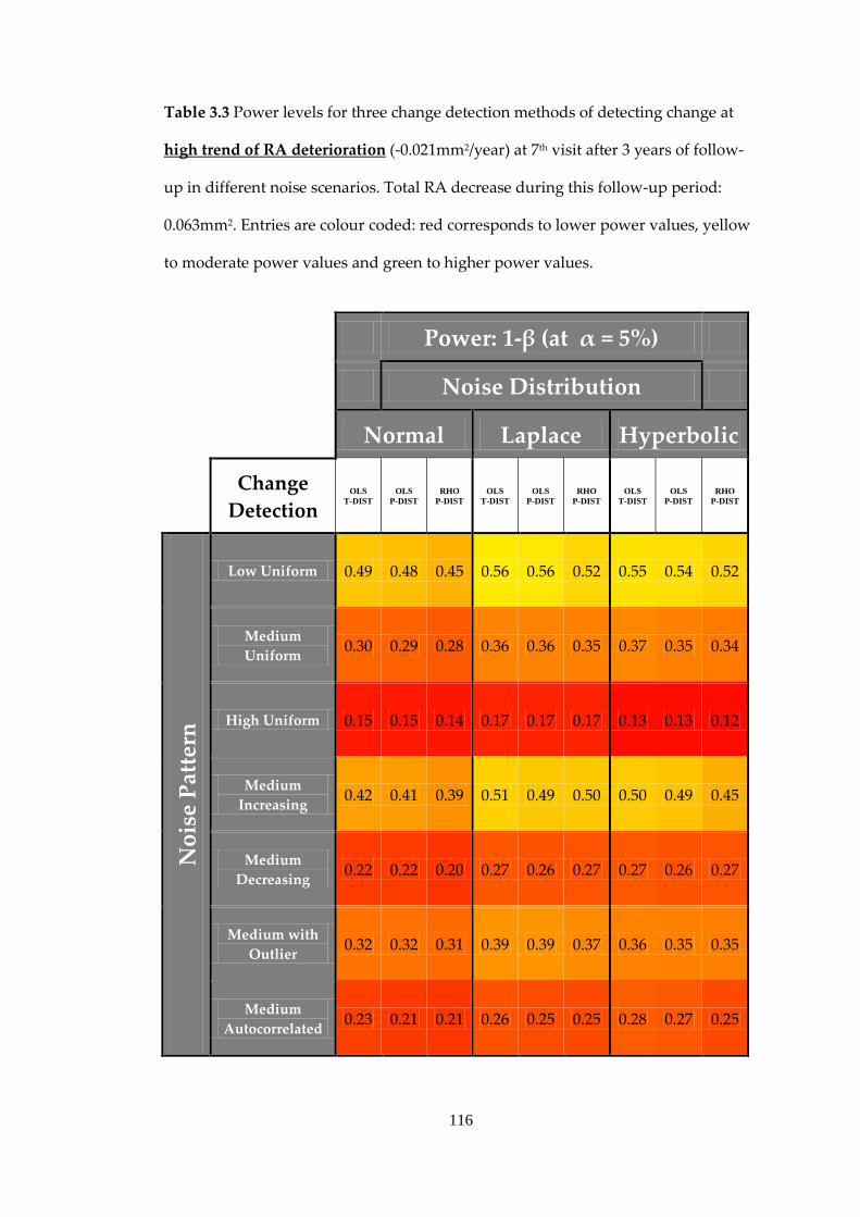
116


high trend of RA deterioration (-0.021mm2/year) at 7th visit after 3 years of follow-

up in different noise scenarios. Total RA decrease during this follow-up period:

0.063mm2. Entries are colour coded: red corresponds to lower power values, yellow

to moderate power values and green to higher power values.


Noise Distribution


Change Detection

OLS T-DIST

OLS P-DIST

RHO P-DIST

OLS T-DIST

OLS P-DIST

RHO P-DIST

OLS T-DIST

OLS P-DIST

RHO P-DIST

Noi

se P

atte

rn

Low Uniform 0.49 0.48 0.45 0.56 0.56 0.52 0.55 0.54 0.52

Medium Uniform 0.30 0.29 0.28 0.36 0.36 0.35 0.37 0.35 0.34

High Uniform 0.15 0.15 0.14 0.17 0.17 0.17 0.13 0.13 0.12





117


medium trend of RA deterioration (-0.012mm2/year) at 13th (and final) visit after 6

years of follow-up in different noise scenarios. Total RA decrease during this follow-

up period: 0.072mm2. Entries are colour coded: red corresponds to lower power

values, yellow to moderate power values and green to higher power values.


Noise Distribution


Change Detection

OLS T-DIST

OLS P-DIST

RHO P-DIST

OLS T-DIST

OLS P-DIST

RHO P-DIST

OLS T-DIST

OLS P-DIST

RHO P-DIST

Noi

se P

atte

rn

Low Uniform 0.80 0.79 0.77 0.82 0.82 0.83 0.82 0.82 0.83

Medium Uniform 0.57 0.56 0.53 0.59 0.60 0.63 0.58 0.57 0.59

High Uniform 0.23 0.22 0.22 0.25 0.26 0.27 0.24 0.25 0.23





118


high trend of RA deterioration (-0.021mm2/year) at 13th (and final) visit after 6 years

of follow-up in different noise scenarios. Total RA decrease during this follow-up

period: 0.126mm2. Entries are colour coded: red corresponds to lower power values,

yellow to moderate power values and green to higher power values.


Noise Distribution


Change Detection

OLS T-DIST

OLS P-DIST

RHO P-DIST

OLS T-DIST

OLS P-DIST

RHO P-DIST

OLS T-DIST

OLS P-DIST

RHO P-DIST

Noi

se P

atte

rn

Low Uniform 1.00 1.00 0.99 0.99 0.99 0.99 0.99 0.99 0.99

Medium Uniform 0.94 0.93 0.91 0.91 0.91 0.92 0.92 0.91 0.92

High Uniform 0.47 0.46 0.46 0.51 0.51 0.54 0.47 0.47 0.45





119

Differences were found for the between trend detection techniques within scenarios

at each visit for AUCs, PAUCs, and power at 5% and 10% to be highly statistically

significant (P<0.0001). Significant statistical differences were found between all

PAUCs of testing strategies at each visit, change magnitude and noise (P<0.0001).

The high sample sizes (N=5000) in each scenario render these statistical inferences

trivial however as the obtained PAUCs are close to their true underlying

(asymptotic) values. Rather in this case the pair-wise differences in between

technique AUCs and PAUCs should be emphasised. The median differences

between PAUC values between methods were as follows: PAUC(OLS T-DIST) –

PAUC(OLS P-DIST) < 0.001; PAUC(OLS T-DIST) – PAUC(RHO P-DIST) = 0.002;

PAUC(OLS P-DIST) – PAUC(RHO P-DIST) = 0.002 with respective interquartile

ranges of 0.003, 0.010 and 0.011. In comparison, values of PAUC (across all

scenarios, visits and techniques) decreased by a median of 10% when uniformly

distributed measurement variability was increased from low to medium, and

decreased by a median of 8% when increased from medium to high. Similarly

PAUC values decreased by a median of 8% when autocorrelation was added to

uniformly distributed measurement variability.

The changes in PAUC values with increasing follow-up examinations in different

scenarios with OLS T-DIST, OLS P-DIST and RHO P-DIST trend detection

techniques are shown for moderate and high trends in Figure 3.5 and 3.6

respectively. The median of the increase in power values at each 6 monthly-interval

for each scenario and technique was approximately 4%.

120



distributions in series of a medium trend of RA deterioration (-0.012mm2/year). The





121



distributions in series of a high trend of RA deterioration (-0.021mm2/year). The





122

Figure 3.7 Two-hundred randomly sampled permutation distributions of OLS linear

regression test-statistics with the parametric Student’s t-distribution (3 degrees of

freedom) overlaid for 4 scenarios of noise pattern: (a) medium uniform noise, (b)

medium increasing noise, (c) medium noise with an outlier and (d) medium noise

with autocorrelation. These distributions are for stable simulated series Laplace

measurement noise at 5th RA measurement (2 years). The average p-value for the

two-sample Kolmogorov-Smirnov test is for (a) 0.78, (b) 0.81, (c) 0.81 and (d) 0.82.

Figure 3.8 Two-hundred randomly sampled permutation distributions of OLS linear

regression test-statistics with the parametric Student’s t-distribution (11 degrees of

freedom) overlaid for 4 scenarios of noise pattern: (a) medium uniform noise, (b)

medium increasing noise, (c) medium noise with an outlier and (d) medium noise

with autocorrelation. These distributions are for stable simulated series hyperbolic

measurement noise at 13th RA measurement (6 years). The average p-value for the

two-sample Kolmogorov-Smirnov test is for (a) 0.52, (b) 0.50, (c) 0.53 and (d) 0.54.

123

3.5 Discussion

In glaucomatous progression, the ability to detect and track trends in univariate

measures such as RA, RNFL thickness, visual field MD and IOP is essential. It is also

important to know how best to detect and measure trends in point-wise analysis

both as pixels in imaging or as testing points in visual fields. Appropriate

techniques should be able to optimally distinguish series of measurements which

exhibit statistically significant trends over time (those series with more reliably

measured deterioration respectively) from those which do not before the clinician

can decide if change is clinically significant or not. The performance of these

techniques will depend on factors such as the number of measurements, length of

follow-up time, the magnitude and structure of measurement variability and the

underlying change. To this end, simulated series were derived with a range of

change and variability parameters in order to establish how well various trend

detection techniques can measure the underlying trends or stability of the series.

Short-term time series of HRT Classic and HRT II derived RA measurement data

were also used as an approximation to stable data to measure the p-value thresholds

of each methods hypothesis test which produce clinically relevant false-positive

rates.

In assessing the alpha-level of these change detection methods, OLS T-DIST yields a

consistently higher 𝛼 at the ~5% and ~10% false positive levels compared to OLS P-

DIST. This means that a ‘less strict’ alpha level needs in OLS T-DIST to be set to

achieve the same level of false positives in this sample of 74 and could infer that

OLS P-DIST is less powerful. The results of the analysis comparing the AUCs and

PAUCs of competing methods show statistically significant differences throughout

between all methods in all noise and signal scenarios at each visit. This is almost

124

wholly due to the high number of virtual patients which reduces the standard error

of the AUC and PAUC estimates. These differences, though statistically significant,

are relatively small for all scenarios. It is not surprising that average AUCs and

PAUCs for all methods increase with an increasing number of measurements

because the power of any test will increase as the magnitude of sampling increases.

There is little literature on the precise nature of RA measurement noise and almost

none on the precise change over time in series of RA. As a result this simulation

model and its interpretation may well only capture some of this information.

However the methodology here has examined a wide spectrum of noise and signal

scenarios using empirical noise parameter estimates where available. Linear and

rank based models of RA change only were examined in this analysis. It may be

argued that a linear model is inadequate to describe the complex process of RA

changes occurring in glaucomatous damage. However, without any evidence of a

more suitable model, it is difficult to justify exploration of an unlimited range of

alternate, more complex models. These models, by design, require more parameters

to define the dependence of the output variable - in this case, RA - on the predictor

variable(s) - in this case, time. This can result in poor statistical power at low sample

sizes and will be particularly at risk of over-fitting models to the data. This is a

modelling error where the model is freer to be closer to each observed point and

ends up fitting the underlying signal in the series but also the measurement noise

itself. In addition these extra parameters may not lend themselves to an instant and

immediate interpretation in a clinic setting.

Though this methodology is very transferrable to measurements derived from other

imaging devices or visual fields, the exact results presented here are those relating

directly to real and simulated longitudinal RA series and should only be interpreted

125

as such. It may be useful in time to model RNFL thickness as derived from OCT or

SLP rather than RA from HRT. The RNFL thickness may well have differing noise

and signal characteristics over time and this should be the subject of further

investigation. It is worth looking at these findings however in comparison to

another example in visual field glaucoma progression research. Monte-Carlo

simulation has been used previously to answer clinically relevant questions in

glaucoma progression detection. Chauhan and colleagues (Chauhan et al., 2008)

reported on the minimum number of equally-spaced visual field examinations

required to detect (with a power of 0.80) a linear trend of -4 dB/year in visual field

mean deviation (summary measure of sensitivity) using estimates of different

degrees of visual field variability. This relied on assumptions that the measurement

errors were identically and normally-distributed and independent. Although

intended to examine RA changes, the analysis of this chapter shows that violations

in these assumptions can considerably affect these reported measurements and that

this is consistent across the change detection techniques investigated. In particular

the effects of autocorrelation, with no-measurable increase in the degree of

variability, on the power to detect an underlying trend are comparable to the effect

of increasing the variability considerably and would change the estimates provided

by Chauhan and colleagues in their report.

The calculated relationship and its significance between the dependent variable and

independent variable (in this case time) in an OLS linear regression (OLS T-DIST)

are based on the assumptions of uniformly, normally distributed measurement

errors and independence of serial measurements. This analysis has tested the

performance of trend detection techniques under violations of these assumptions:

changing magnitude of variability with time, correlations between the

measurements over time and non-normal distributions of noise. The autocorrelation

126

of serial measurements as modelled in this analysis had a large effect on the

performance of all methods. This is to be expected for the OLS T-DIST method as

the standard error of the slope/trend will be systematically underestimated. This

also occurs for the permutation framework for both linear and rank based methods.

Previous research has shown that resampling methods which do not take into

account the serial correlation of the dependent variable can underestimate the

standard error of Spearman’s 𝜌 (Park and Lee, 2001) which would again decrease

the performance.

If the number of data points is small, it may be difficult to detect assumption

violations. With small samples, violation assumptions such as non-normality or

heteroscedasticity of variances are difficult to detect even when they are present.

With a small number of data points linear regression offers less protection against

violation of assumptions. With few data points, it may be hard to determine how

well the fitted line matches the data, or whether a nonlinear function would be more

appropriate. Since parameter estimation is based on the minimization of squared

error, a few extreme observations can exert a disproportionate influence on

parameter estimates. Calculation of confidence intervals and various significance

tests for coefficients are all based on the assumptions of normally distributed errors.

If the error distribution is significantly non-normal, confidence intervals may be too

wide or too narrow.

The results of this analysis suggest that for data which can be modelled as presented

there is little difference in the three methods of analysis investigated. One crucial

assumption, that progressive RA damage followed a linear trend, was not altered in

this simulation and this may offer more promise for a rank-based method which

shows relative efficiency almost equal to linear trend detection methods. In cases of

127

non-linear trends, a rank-based method is likely to prove more powerful in

detecting this underlying trend. In consideration of these factors, a rank based

approach may provide the best option of these three approaches. If these time series

are representative of longitudinal RA measurements of a large set of virtual patients

then these inferences can also be applied to real data scenarios. Further

characterisation of RA and topographic variability are required as are predictors of

these.

128

4. Assessment of Quality in

HRT Images

Image quality assessment gives important clinical information on the fidelity of

rendered images. The quality of an image is important and sometimes crucial in

clinical decision making as the example case of Figure 4.1 shows. From a neuro-

radiological study (Phal et al., 2008), this case involved a patient with a brain lesion

symptomatic of epilepsy and normally indicated by a higher intensity (higher tissue

density) scan value in MRI. This lesion was not identified in an initial lower quality

scan but was evident in a secondary improved quality scanning modality. The first

scan was acquired using an MRI scanner with a magnet of lower flux (units in Tesla

or T) than the scanner used for the second scan. Image quality has been shown in

other studies to vary considerably between MRI scanners with magnets of differing

operating flux (Beyersdorff et al., 2005, Kataoka et al., 2007).

In the context of examining retinal images with application in glaucoma detection

and tracking over time image quality metrics can inform the clinician or automated

algorithm how much or how little confidence to place in a measurement derived

from a particular image. In assessing the overall quality of a medical image factors

such as the optical resolution of the scanning or imaging system, the noise inherent

in the measuring system, the contrast of the image and the presence of artefacts in

the image must be accounted for.

129

Figure 4.1 MRI scans of patient with intractable nocturnal seizures. (a) Coronal

image using 1.5-T magnet MRI showing questionable curvilinear focus of high

signal intensity (arrows). Abnormal signal intensity was missed at first review of

images. (b) Coronal image using 3-T MRI showing curvilinear band of high signal

intensity (arrows) white matter without apparent mass effect. (Reproduced from

(Phal et al., 2008))

The image quality of a given HRT mean topography is measured with the MPHSD;

a metric provided by the HRT software as an assessment of the within examination

variability across three single topographies. The HRT software also gives other

assessments of image quality at the time of acquisition. It provides a list of ‘pass’ or

‘fail’ checks for appropriate accommodation and camera distance, for sufficient

image brightness and image illumination and for levels of eye movement, blinks,

fixation loss and eye drift below tolerable levels (Figure 4.2). Once a scan has passed

these criteria, it is the MPHSD which dictates the post-acquisition assessment of

image quality. The manufacture provided guidelines for interpreting the quality of a

resultant MPHSD value of a mean topography are summarised in table 4.1.

130

Figure 4.2 Example output of image quality assessment by HRT software of the

constituent images in a HRT mean topography.

MPHSD as provided by the HRT software is actually the calculated geometric mean

(not the arithmetic mean) of the sample standard deviation of each pixel in the mean

topography image across the three constituent single topographies. As an

illustration, if a sample contains 𝑛 measurements 𝑎𝑖 the more familiar arithmetic

mean 𝜇𝑎 is calculated as follows:

𝜇𝑎 = 𝑎1+𝑎2+𝑎3+⋯𝑎𝑛𝑛

,

and the geometric mean 𝜇𝑎 is calculated as follows:

𝜇𝑔 = �𝑎1𝑎2𝑎3 …𝑎𝑛𝑛 .

The geometric mean is less affected by long tails in negatively and positively

skewed distributions (Altman, 1999).

131

Table 4.1 Instrument guidelines categorising MPHSD (courtesy of Heidelberg

Engineering, Heidelberg, Germany)

MPHSD (µm) Category Description < 20 1 Very good

20 - 30 2 Good

30 - 40 3 Acceptable

40 - 50 4 Look for way to improve

> 50 5 Low quality (do not use as baseline image)

MPHSD has been shown to be affected by media opacities due in part to aging and

cataracts (Zangwill et al., 1997, Strouthidis et al., 2005b). This has been quantified

with significant correlations of the MPHSD to scores of the severity of opacities of

various types and at various locations in the eye using the Lens Opacities

Classification System III (Chylack et al., 1993). In the first of these studies (Zangwill

et al., 1997), an observer panel assessed, on a ten point scale, the quality of the 3 x 32

constituent CSLO optical sections composing a mean topography on 39 subjects.

Here, significant correlation of the subjective image quality of the scanned pre-

processed CSLO images to the MPHSD was strong (𝑟2=0.76). This is because in

cases with high noise (light scatter) during the acquisition of CSLO optical sections,

there will be inherit difficulties in accurately determining the position of maximum

reflectance, and hence calculating the topographic height. Another study has shown

MPHSD to be strongly correlated to the camera sensitivity of the device and

spherically corrected astigmatism but not with age however (Sihota et al., 2002)

though subjects with media opacities were excluded from this study.

Previous studies have used the MPHSD as a metric to evaluate the repeatability of

the technology in normal subjects and glaucoma patients (Chauhan et al., 1994,

132

Rohrschneider et al., 1994). Most previous studies of detection of glaucoma in HRT

images have used this metric as a criterion in selection of data for analysis. Below

the 50µm threshold for acceptable images (table 4.1) evidence suggests that the

diagnostic capability of the HRT is unrelated to MPHSD (Sung et al., 2009). Many

studies have used 50µm as a cut-off for including or excluding images (Medeiros et

al., 2006, Coops et al., 2006, Saito et al., 2009, Burgansky-Eliash et al., 2007) and

others have used 40µm (Harizman et al., 2006, Zelefsky et al., 2006). The problems

of screening a normal elderly population (aged 65 to 89 years) with HRT have been

highlighted in a study containing 880 individuals which reported that 29% of

images from subjects in a normal elderly population had MPHSD >50µm and were

thus excluded from the study (Hawker et al., 2006). In this same study 53% of 95

glaucoma patients were also excluded due to MPHSD values >50µm.

Studies of glaucomatous progression detection in HRT images have employed

MPHSD as an image quality selection filter (Kourkoutas et al., 2007, Bowd et al.,

2009) using 50µm as a cut-off for selection. Another study has used a MPHSD of

<35µm and iterative change in MPHSD between visits of <10µm as selection criteria

for analysis (Saarela and Airaksinen, 2008) accounting for an exclusion of 18% and

16% respectively of eyes from the study.

MPHSD has been shown to be a good predictor of variability in stereometric

parameters (Sihota et al., 2002) and in particular of variability in longitudinal and

test-retest RA measurements (Owen et al., 2006) and as a means of stratifying and

optimising progression analyses of these parameters (Fayers et al., 2007). The

interpretation of MPHSD as with any image quality metric should be clear and

consistent. Achieving a better understanding of factors influencing it and its

133

implications for the reliability of mean topography derived data is worthwhile both

in clinic and for research studies.

The aim of this chapter is to investigate if the characteristics of topography and

reflectance images before alignment and averaging affect the resulting variability of

mean topography images. To do this an examination of simulated data in addition

to an examination of real data is performed. Frequency domain (using Fourier

analysis) and image gradient metrics are compared in both these simulated and real

data to MPHSD values. Independent subjective grading of topography and

reflectance image pairs by a group of experienced users of the HRT are also

compared to MPHSD values. The agreement of the subjective assessments between

graders was also quantified to measure the need for an objective quality metric of

HRT images.

The work in this chapter was presented at the Image Morphometry and Glaucoma

in Europe Meeting, Mannheim, Germany on January 13-14, 2006 and the

Association for Research in Vision and Ophthalmology Meeting, Fort Lauderdale on

April 30 - May 4, 2006.

134

4.1 Measurements of Image Variability

For this study, global variability is quantified using the MPHSD and local variability

is quantified using PHSD maps and distributions. Real data acquired across a large

range of imaging conditions are used for analysis. Simulated data are also used to

test the specific hypothesis that the same misalignment noise applied to different

images produces variability dependent upon characteristics of the initial image. This

hypothesis has important clinical implications because two different eyes may have

images that exhibit exactly the same amount of measurement noise but may yield

very different MPHSD values because the features in the images are different. In

HRT topography images these characteristics can be related to the underlying

morphology of the ONH and the imaging quality of the optics of the eye.

4.1.1 Real Data

In examining quality of HRT image data, the topography and reflectance images of

74 eyes of 74 subjects from the same study detailed in Chapter 3 are analysed. In

particular HRT Classic, baseline mean and (three) single topography and reflectance

images of each selected eye are examined. As discussed previously, this dataset of

images was deliberately enriched with eyes having a range of media opacities and

thus the image quality range would also be expected to be large. The MPHSD

values of all 74 topographies are calculated and outputted using the HRT Classic

software. The PHSD maps of all 74 topographies are also calculated from the raw

single topographies. Inter-quartile ranges are calculated for all PHSD distributions

to quantify the ‘spread’ of these distributions. Examples of PHSD maps are shown

for given mean topographies in Figure 4.3 along with the distribution of PHSD

values.

135

Figure 4.3 Sample mean topographies (a) and (d) with respective PHSD maps (b)

and (e). PHSD distributions (c), (f) are also displayed. MPHSD values are 15µm and

30µm for (a) and (b) respectively.

MPHSD is also further examined as a predictor for two types of RA variability:

overall series variability and the contribution of an individual topography’s RA

deviation to the variability of RA measurements in a series. The relationship of

MPHSD to overall series variability is assessed by simply comparing the standard

deviation of the 5 RA measurements to the mean MPHSD in the 5 mean

topographies for each patient. Secondly, the predictive value of MPHSD values in

identifying outlier measurements in a given series is examined. Firstly, the mean of

the 5 values of RA is calculated and used as a best available estimate of the true RA

for each patient. This mean is subtracted from each of the 5 individual RA

measurements to give 5 deviations from the mean for each patient. These deviations

are then normalised (dividing by the standard deviation of the 5 RA measurements)

as a way to quantify the proportion or contribution of each RA measurement to the

136

overall series RA variability. The five normalised deviations are then compared to

the 5 matching MPHSD values normalised by the average MPHSD.

4.1.2 Simulated Data

The simulated images are derived in a similar fashion to a previously published

approach (Patterson et al., 2005) Here, post-processed single topographies are used

as seeds to propagate simulated single topographies and from these serial mean

topographic images are derived. Noise, approximately mimicking the noise inherent

in mean topography formation, is applied to the single seed topography producing

simulated single topographies in a given series. The method for simulating images

with known properties involved synthesising new single topographies from one

‘seed’ single topography by applying various types of noise. Firstly, random, small

transformations composed from translational, rotational, shear and scaling

parameters are applied to a seed single topography. Some of these transformations

are visualised in Figure 4.4.

White noise (spatially independent pixel Gaussian noise) is added to each

misaligned single topography with each pixel chosen from a zero-centred, normal

distribution: 𝑁(0,𝜎). The small random transformations along with white noise

can be used to approximately model the main noise (sources of variability) at the

image. The spread of each distribution from which each randomly sampled

transformation parameter is sampled is estimated by trial and error. This is because

it is impossible to measure the residual movement error that remains after the HRT

alignment algorithm has been applied to all single topographies when forming a

mean topography. Further details of how each transformation is implemented and

137

the probability distributions for parameters involved in each transformation are

given in Appendix B.

Figure 4.4 Sample HRT Classic topography displayed in three dimensions with

reflectance intensity colour mapping. Misalignments due to translations

�𝑡𝑥, 𝑡𝑦 , 𝑡𝑧� along and rotations (∅,𝜌,𝜃) about the (𝑥,𝑦, 𝑧) axes are shown.

Measurements and translations in the 𝑧-axis are referred to as axial and those in the

𝑥𝑦 plane as transverse.

This simulated noise is applied to 74 single topography images, each from the

baseline scan of an eye included in the real dataset. A simulated set of 3 single

topographies is generated for each ONH by the application of an identical set of 3

noise components to each of the single topographies. It is from these 74 sets of 3

single topographies that 74 mean topography images are generated. The associated

138

individual pixel height standard deviation (PHSD) values are calculated at each

pixel in all mean topographies. From these, a MPHSD value is calculated for the

corresponding mean topography. For the purposes of examining the effect of

misalignment and white noise on mean topography formation, noise applied across

all seed single topographies is, therefore, controlled to be the same for each

generation of a simulated single topography. This is demonstrated in Figure 4.5 for

two sample series/seed single topographies.

The simulation was performed 50 times, creating 50 mean topographies for each

eye. Thus, when averaged over many simulations, it becomes possible to examine

the dependence of the MPHSD metric on the characteristics of the seed

topographies alone.

Two types of simulated noise will produce variability independent of the image

itself. These are axial translations and white noise. In an attempt to identify a

minimal level of noise which is independent of the optic disc morphology, different

combinations of white noise and axial translational noise (by varying parameters 𝜎

and 𝑡𝑧) are applied to ‘blank’ images (pixel values=0) the same size as HRT Classic

single topographies (256 x 256) to produce MPHSD values. The assumption is made

that the minimum MPHSD values observed in the real mean topography data will

be mostly occurring in well-aligned, ‘low feature’ images. Under this assumption,

values for 𝜎 and 𝑡𝑧 are selected to produce this minimum MPHSD. Different

MPHSD values for varying parameters 𝜎 and 𝑡𝑧 are plotted in Figure 4.6. The

minimum observed MPHSD value (see section 4.3 and Figure 4.10) observed in this

study’s real mean topographies would thus be used to determine what values to

choose for parameters 𝜎 and 𝑡𝑧 along with the results in Figure 4.6.

139

Figure 4.5 The simulation schematic with three different, random misalignment and

noise sets applied to a seed single topography to produce three simulated single

topographies for two sample eyes. In this example each set applied is identical for

both eyes and this is the case across all seed topographies in the analysis.

As previously stated, it would be impossible to measure any post-alignment

remaining misalignment. The simplifying assumption is made that the simulated

misalignments and noise are close to the residual misalignment after registration

between real single topography and reflectance images. Thus these transformations

are small enough to not require re-alignment as would be the case for real data. As

single reflectance images are only used in the alignment stage (see Section 1.2) of

140

image formation of the mean topography and thus the MPHSD, they are not

analysed for simulated data.

Figure 4.6 The relationship of MPHSD of a 256 x 256 ‘flat’ image with different

levels of morphologically independent noise added. Boundary points where

MPHSD values are produced corresponding with the minimum MPHSD observed

in real data (10µm) are indicated.

141

4.2 Measurements of Image Characteristics

Three approaches are used in measuring the relationship of the MPHSD to image

characteristics of the reflectance and topography images. These approaches use

information about (i) the underlying spectrum in the images, (ii) the gradients in the

images and (iii) the quality assessment of a panel of experienced HRT users.

4.2.1 Image Frequency Analysis

In image processing, Fourier analysis is a standard tool for examining, modifying

and characterising images. Its theoretical basis is that any signal can be

decomposed, using a Fourier transform, into a series of component sinusoidal signals

of different frequencies and amplitudes and this can be represented in the frequency

domain. In the frequency domain the amplitudes of the signal’s various component

frequencies can be represented in a power spectrum and this allows an examination of

the relative amounts of each frequency component in a signal. In a one-dimensional

signal, such as a sound or an electrical signal, the power spectrum is one-

dimensional and the frequencies related to time (the signal changes with time). For a

two-dimensional signal, as in the case of an image, the power spectrum is two-

dimensional with the direction of the frequency component indicated along with its

amplitude (see Figure 4.7 and Figure 4.8 (a)-(d)). These frequencies are related to

spatial units (the image changes with position). An illustrative simple case is shown

in Figure 4.7 where (a), (b) and (c) are images of vertical bars, a face and a galaxy

respectively. In (a), there are no features in the vertical axis so the power spectrum

(d) contains frequency amplitudes on the horizontal axis only. It is often easier to

objectively characterise the type and number of features and the noise present in

images and to quantify underlying differences between images in the frequency

142

domain and this is illustrated in Figure 4.7. More technical details on Fourier

analysis in image processing can be found in (Bovik, 2009) and (Smith, 2003).

Fourier analysis is performed on each of the three constituent single topography

images of a mean topography image for real data and on the seed single topography

images for simulated data. As the reflectance image is used for alignment in the

HRT software, Fourier analysis is also performed on the three constituent single

reflectance images of a mean reflectance image for real data. It has been shown that

different types of images can be categorised by their Fourier power spectra

(Torralba and Oliva, 2003). In particular, images of natural scenes have been shown

to have characteristic power spectra (Ruderman and Bialek, 1994). The summed

spectral magnitude density of each image is calculated (average of the power

spectrum across all pixels except the 0th frequency representative of the average

intensity of the image). The radial-averaged spectrum density (RASD) of each

appropriate image is calculated. This involves averaging all possible directional

power spectra in discrete radial intervals and provides a convenient means to

compare two dimensional spectra in one dimension. The RASD centroid is

calculated to indicate the frequency at which 50% of the spectral energy is

distributed on either side; it is analogous to a median of a distribution or the ‘centre

of mass’ of the RASD and has previously been used for dimensional signals used as

a means of characterisation in music perception (Schubert et al., 2004), where it has

been shown to correlate well with the perceived timbre in experiments using

computer-generated multiple instrument sounds. It is also used, among other

measures, as an indicator of the depth of anaesthesia when monitoring patient

electroencephalogram (EEG) readings during surgery (Schwender et al., 1996,

Nieuwenhuijs et al., 2002, Drummond et al., 1991); in this field it is referred to as the

spectral edge frequency. Examples of topographic and reflectance images, their

143

respective power spectra and RASD along with the centre of mass analysis are given

in Figure 4.8.

Figure 4.7 Fourier analysis example of (a) an image with periodic vertical stripes, (b)

photograph of Pádraig Mac Piarais in side profile, (c) telescope image of the M91

galaxy, (d) power spectrum of (a), (e) power spectrum of (b), (f) power spectrum of

(c). The brighter the points in (d), (e) and (f) indicate the higher amplitude of a

given frequency - lower frequencies are located towards the centre of these images

and higher frequencies towards the edges. Note that log scales for the intensity are

used for (d), (e) and (f) as the proportions of frequency components at the centre

(representing the average of the signal) and at key characteristic frequencies are

much higher than elsewhere.

144

Figure 4.8 Fourier analysis, example of (a) single topography image, (b) single

reflectance image, (c) magnitude of frequency spectrum of single topography image,

(d) magnitude of frequency spectrum of single reflectance image, (e) RASD (dashed

lines) with solid vertical lines representing the centroid for the reflectance and

topography images. The position of each RASD centroid is also marked on images

(c) and (d).

145

4.2.2 Image Gradient Analysis

Fourier analysis will provide an estimate of how global characteristics of the image

influence MPHSD measures. The occurrence of higher or lower variability at certain

spatial locations in a HRT image should also be described and accounted for.

Previous studies have qualitatively noted the matching locations of anatomical

features such as vessels and the ONH cup margin in HRT topographies with

relatively higher locations of variability across single topographies composing a

mean topography (Chauhan et al., 1994, Chauhan and McCormick, 1995).

One study (Brigatti et al., 1995) calculated “steepness” maps measuring local spatial

variability and variability across single topographies (in a 3 x 3 x 3 pixel

neighbourhood) at each pixel. Some correlation between the matching pixel

locations of the steepness maps and the PHSD maps was reported. The calculation

of these steepness maps however was limited as it ignored the potential spatial

nature of the variability in the pixel neighbourhood. In addition by including the

variability across single topographies in the steepness calculation it did not make a

valid calculation of the local spatial variability.

A preferable approach would be to calculate the gradients along transverse 𝑥 and 𝑦

axes at each pixel for each single topography and reflectance image. The combined

square root of the mean squared sum of these two gradient components is

calculated to provide a scalar value representing the local gradient magnitude (GM)

about each pixel. The GM can be visualised as the maximum slope magnitude of a

plane fitted to the 3 x 3 pixel neighbourhood about each pixel.

146

Figure 4.9 Gradient analysis, example of (a) mean real topography PHSD map, (b)

mean simulated topography PHSD map, (c) average GM map of constituent real

single topography images, (d) GM map of seed single topography image, (e)

average GM map of constituent real single reflectance images. For real data, cross-

correlation coefficients are 0.41 between maps (a) and (c) and 0.25 between maps (a)

and (e). For simulated data, cross-correlation coefficients are 0.64 between maps (b)

and (d). Note: Grey-scale maps have equal ranges across rows of this Figure but not

along columns.

147

For a given mean topography, the GM maps for all constituent single topographies

and related single reflectance images are compared to the related PHSD map using

image cross-correlation. The similarity of two images by cross-correlation is

quantified by the maximal, normalised cross-correlation coefficient. For simulated

data, as no reflectance images are involved in the generation of a simulated mean

topography, only GM maps of the seed single topographies are compared to PHSD

maps. An example of this analysis for real and simulated data is given in Figure 4.9.

4.2.3 Subjective Assessment

Six experienced users of the HRT, including glaucoma fellows and glaucoma

specialists (referred to as graders) were presented with 28 PowerPoint slides, each

containing a sample HRT reflectance and topography image displayed as a pair.

These 28 image pairs were chosen on a semi-random basis - it was required that

they be representative of the image quality distribution in the overall sample - and

the MPHSD distribution in this sub-sample was compared to the MPHSD

distribution in the overall sample. Graders were asked to classify the quality of each

image pair on a discrete scale of 1 to 5. Score 1 is described as ‘Best’ quality and

score 5 as ‘Worst’ quality. No other criteria were given for image quality

assessment. The graders were asked to repeat this scoring with the same series in a

randomised order and blind to their previous scores. A linearly weighted Cohen’s κ

score is used to measure the pair-wise agreement between all observers and within

observers.

A panel score is also calculated for each image pair from the mean of each

observer’s mean score. These panel scores are compared to MPHSD values to assess

the correspondence between the clinician’s confidence in image quality and the

objective measurement of MPHSD. Frequency and gradient metrics as described

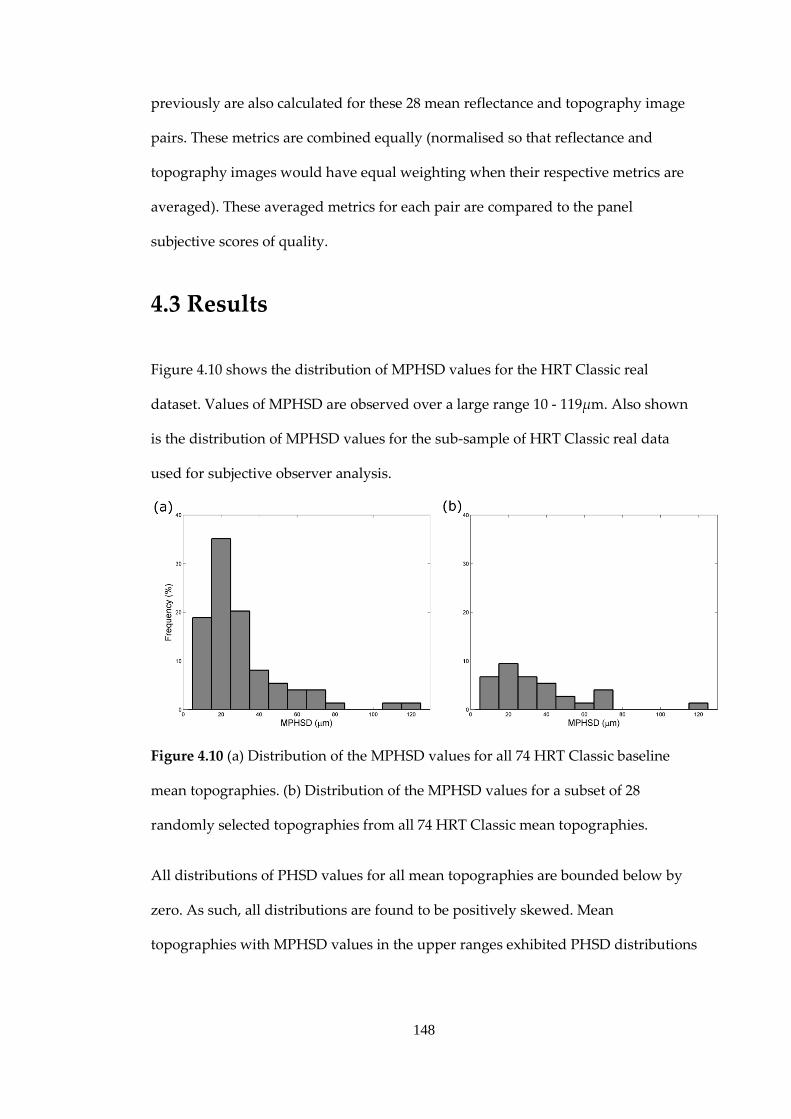
148

previously are also calculated for these 28 mean reflectance and topography image

pairs. These metrics are combined equally (normalised so that reflectance and

topography images would have equal weighting when their respective metrics are

averaged). These averaged metrics for each pair are compared to the panel

subjective scores of quality.

4.3 Results

Figure 4.10 shows the distribution of MPHSD values for the HRT Classic real

dataset. Values of MPHSD are observed over a large range 10 - 119µm. Also shown

is the distribution of MPHSD values for the sub-sample of HRT Classic real data

used for subjective observer analysis.

Figure 4.10 (a) Distribution of the MPHSD values for all 74 HRT Classic baseline

mean topographies. (b) Distribution of the MPHSD values for a subset of 28

randomly selected topographies from all 74 HRT Classic mean topographies.

All distributions of PHSD values for all mean topographies are bounded below by

zero. As such, all distributions are found to be positively skewed. Mean

topographies with MPHSD values in the upper ranges exhibited PHSD distributions

149

with a larger spread (as assessed by the IQR) than those of lower MPHSD values

(Figure 4.11).

Figure 4.11 MPHSD values compared to inter-quartile range (IQR) values for PHSD

distributions.

Figure 4.12 shows the effects of MPHSD on RA variability. For the series average

setting (a), a strong linear relationship is observed between series RA standard

deviation and the series averaged MPHSD: Pearson’s sample correlation coefficient,

𝑟=0.59 (p<0.001). For the individual image setting (b), only a very weak linear

relationship is observed between the individual image MPHSD as a fraction of the

mean series and the image deviation from the RA best available estimate (series

mean RA) as a fraction of series RA standard deviation (Pearson’s rank correlation

coefficient, 𝑟= 0.15 p=0.003).

150

Figure 4.12 (a) Series RA standard deviation values plotted against series-averaged

MPHSD values. (b) The magnitude of difference of individual RA measurements

from the series RA best available estimator (BAE) - as calculated by the series

average RA measurements – as a fraction of series RA standard deviation plotted

against MPHSD values as a fraction of series-averaged MPHSD values. Areas of a

higher density of points are represented by darker shading.

For the simulation, the range of MPHSD values varied considerably (18 – 116µm)

despite identical noise being applied to generate all mean topographies. The range

of MPHSD values for simulated data is similar to that of real data but poor

agreement is observed with increased real mean topography MPHSD values as seen

in Figure 4.13.

151

Figure 4.13 MPHSD values for real and simulated mean topographies. The

minimum observed MPHSD (10µm) in real mean topographies is plotted as a lower

bound for simulated mean topography MPHSD. Pearson’s sample correlation

coefficient 𝑟: 0.79 (p<0.001), MPHSD real – MPHSD simulated mean: 7.6 µm,

standard deviation: 13.7 µm.

Fourier analysis revealed a strong significantly positive dependence of the MPHSD

value on the RASD centroid and the summed spectral magnitude density of “pre-

averaged” single topography for both real and simulated data. Simply put the

MPHSD of mean topographies is affected by the characteristics of the component

images. In addition, for real data, there is a strong significantly positive dependence

of the MPHSD value on the RASD centroid and a negative dependence of the

MPHSD on the summed spectral magnitude density of “pre-averaged” single

topography for both real and simulated data. Figure 4.14 illustrates these

relationships.

152

Figure 4.14 Fourier metrics of constituent single images compared to MPHSD

values. Pearson’s 𝑟 correlation coefficients are for (a) 0.74, (b) 0.93, (c) 0.69, (d) -0.55,

(e) 0.58 and (f) 0.58.

Figure 4.15 Measure of the average GM of constituent single images compared to

MPHSD values. Pearson’s 𝑟 correlation coefficients are for (a) 0.95, (b) -0.51 and (c)

0.85.

153

Figure 4.16 Distributions of (a) averaged measure of the NCC of real mean

topography PHSD maps and GM maps for each constituent single topography (b)

averaged measure of the NCC of real mean topography PHSD maps and GM maps

for each constituent single reflectance image and (c) averaged measure of the NCC

of multiple simulated mean topography PHSD maps and GM maps for single seed

topographies. Means of distributions are 0.375, 0.25 and 0.56 for (a), (b) and (c)

respectively.

Both locally and globally, there is a measurable relationship of MPHSD to image

gradient measures of “pre-averaged” single topographies. On a global scale, for

simulated data and real data, there is a strong positive relationship between GM

mean values averaged across single topographies and MPHSD values. For real data,

there is also a negative relationship between the GM mean values averaged across

single reflectance images and the MPHSD. Figure 4.15 displays these relationships.

On a local scale means of NCC values in comparing maps of PHSD maps and GM

maps of single topography and reflectance images are 0.37 and 0.25 respectively for

real data. For simulated data, the mean of NCC values for comparisons of PHSD

maps and GM maps of single topographies is 0.45. NCC distributions for all 74

scans are presented in Figure 4.16.

154

Within and between-observer agreement among clinicians quantified by linearly

weighted κ values are shown in table 4.2 including mean between observer

agreement and mean within observer agreement (repeatability).

Table 4.2 Agreement between the subjective assessments of the image quality of

HRT mean topography and reflectance image pairs by 6 observers (A – F). Quality

assessments were made over a subset of 28 image pairs. Agreement is quantified by

use of linearly weighted κ values. Observers were asked to repeat their quality

assessments on the same (but reordered) subset (1 – 2). Within observer agreements

are in indicated by the italic font. The strength of agreement is indicated by colour -

red represents the lowest agreement and green the highest.

Observer

A1 A2 B1 B2 C1 C2 D1 D2 E1 E2 F1 F2

A1 0.78 0.58 0.75 0.37 0.51 0.50 0.61 0.61 0.53 0.61 0.52

A2 0.61 0.78 0.49 0.59 0.62 0.64 0.55 0.57 0.65 0.65

B1 0.67 0.45 0.49 0.63 0.66 0.37 0.36 0.54 0.48

B2 0.54 0.60 0.58 0.70 0.52 0.59 0.81 0.66

C1 0.76 0.51 0.53 0.26 0.46 0.64 0.61

C2 0.59 0.60 0.41 0.62 0.79 0.69

D1 0.82 0.38 0.41 0.55 0.48

Median Within Observer

D2 0.48 0.51 0.66 0.50

0.76

E1 0.62 0.47 0.42

Median Between Observer

E2 0.64 0.58

0.58

F1 0.75

F2

155

The relationship between observer image quality panel scores and MPHSD values is

displayed in Figure 4.17 (a). Equally weighted combined Fourier metrics (RASD

centroid) and gradient metrics (mean GM) for reflectance and topography image

pairs are plotted in Figures 4.17 (b) and (c) respectively. Examples of four mean

topography and reflectance image pairs are given in Figure 4.18. The associated

panel scores, the standard deviation of observer scores (averaged over repeat

assessments) and MPHSD values are also included.

Figure 4.17 Subjective observer assessed panel scores of image quality of mean

topography and reflectance image pairs compared to (a) MPHSD, (b)

reflectance/topography image combined RASD centroid measurement and (c)

reflectance/topography image combined mean GM. Coloured points on figures

correspond to those examples in Figure 4.18. Pearson’s 𝑟 correlation coefficients are

for (a) 0.81 (b) 0.81 and (c) 0.28.

156

Reflectance-Topography Image Pair Mean Panel

Score (Rounded)

MPHSD (Category)

Panel Score SD

Plot Symbol

1.42

(1)

18µm

(1) 0.51

4.83

(5)

38µm

(3) 0.39

4.92

(5)

121µm

(5) 0.29

3.92

(4)

51µm

(5) 0.90

Figure 4.18 Examples of reflectance-topography image pairs (a)-(b), (c)-(d), (e)-(f)

and (g)-(h) presented to experienced Heidelberg Retina Tomograph operators with

mean panel scores (rounded to nearest category) and standard deviation of scores

across all observers. MPHSD values and manufacturer supplied categories for these

values are displayed. Coloured symbols are used to represent these examples in

Figure 4.15. (SD: standard deviation).

157

4.4 Discussion

In case finding using medical images, a measurement of image quality is necessary

to assess how adequate any evidence (or lack thereof) in the image is for diagnostic

purposes. The effect of a degraded image quality on clinical decision making is

illustrated in the opening example of Figure 4.1, a case no doubt where a metric

showing poor image resolution would have perhaps led to an immediate second

scan in the first review of the patient. In the assessment of glaucomatous

progression, the confidence in any change detection algorithm will need to

incorporate an objective, easily understandable measure of image quality which is

robust and accurate on a local and global scale.

Below the 50µm threshold for acceptable images evidence suggests that the

diagnostic capability of the HRT is unrelated to MPHSD (Sung et al., 2009). Image

quality assessments in glaucoma detection and monitoring of structural changes in

the retina and ONH are not just relevant to HRT imaging. RNFL assessments using

OCT have been shown to be significantly affected by image quality; measurements

of RNFL thickness have been shown to be correlated to image quality metrics (Sung

et al., 2009, Balasubramanian et al., 2009).

The results of this and previous studies (Owen et al., 2006, Sihota et al., 2002) show

that high average MPHSD values for a series of HRT derived RA measurements are

predictive of higher RA variability. However this study also found that, in a series

itself, a mean topography with a relatively higher MPHSD value than the other

mean topographies had little relatively higher contribution to RA variability in that

series. In the context of glaucoma progression studies, these findings mean that a

series of RA measurements can be more helpfully assessed with the MPHSD as an

158

indicator of the overall series variability; this concept has been used in a previous

study to optimise a HRT RA progression analysis (Fayers et al., 2007). Conflictingly,

a MPHSD measurement of a mean topography may serve little use as an individual

weighting parameter for its associated RA measurement in analyses of change such

as a weighted least squares regression or a Chi-squared regression of RA over time

or in the identification of outlier RA measurements in a series.

The MPHSD values of mean topographies of different ONH and surrounding area

morphologies in different scanning conditions (due to different media opacities and

aberrations) fall within a large range. Significantly, a large component of this

variability is due to the underlying characteristics of the pre-averaged single

reflectance and topography image sets. In short, the MPHSD is affected by the

features in the pre-averaged images and is therefore not a wholly independent

measure of image quality. MPHSD values are higher for mean topographies whose

constituent single topographies produce higher image metrics indicating the

amount of signal ‘energy’ (spectral density magnitude sum), and the image-

averaged localised gradient about each pixel (mean GM). This has implications for

the clinical use of this metric, especially when it is used, for example, in population

based studies as a threshold upon which patients are included or excluded.

A simulation was developed to illustrate that, when equal misalignment noise is

used to generate new single topographies, a systematically large range of MPHSD

values of the resulting simulated mean topographies values is demonstrated. This

confirms that misalignment noise interacts with the single topography structure in

producing MPHSD values: MPHSD is not a true measure of misalignment noise

between single topographies. Quantitative evidence is also provided of the

relationship of pixel neighbourhood gradient maps of single topographies and the

159

PHSD maps i.e. evidence of the correspondence between local areas with high

gradients (or edges) and high PHSD areas. This leads to the somewhat obvious

conclusion that ‘movement’ applied to less ‘flat’ images, with less homogeneity,

will result in higher global variability due to increased local variability in the

locations of higher gradients.

Where the directionally-independent median frequency of the spectral density

magnitude distribution (RASD centroid) is higher in single topography and

reflectance images the MPHSD of mean topographies is also higher. From this one

can infer that the higher the proportion of high frequencies in a single topography

set, the higher the MPHSD for the resulting mean topography. These high

frequencies can come from real structures such as the sharp edges of vessels and the

cup/rim margin but also from image acquisition background noise from light scatter

in eyes with high levels of media opacity.

The HRT alignment software uses the features in single reflectance images to assess

how best to align single topographies before averaging to form a mean topography.

Some reflectance image metrics (spectral density magnitude sum and mean GM) are

negatively correlated to MPHSD values. This suggests that, the higher the values of

these metrics, the higher likelihood that features in reflectance images are correctly

detected and single topographies are better aligned reducing the MPHSD.

Observers, even those trained to use the HRT and interpret its output data, can have

poor agreement with each other (weighted Cohen’s 𝜅 lower limit of 0.26 and

median of 0.58) in assessing the quality of output HRT topography and reflectance

image pairs. Moreover, the repeatability of image quality judgements by expert

observers is only moderate (median 𝜅=0.76) as measured by agreement with a

160

second grading of the same set of image pairs by each observer. The between-

observer median 𝜅 value in this study is comparable to the between-observer

median unweighted Cohen’s 𝜅 of 0.55 in a study of clinicians assessment of the

quality of 100 fundus photographs (Bartling et al., 2009). Both between-observer and

within-observer agreement measures for HRT image quality grading are no better

than the decisions of clinicians when assessing monoscopic and stereoscopic

photographs for the presence of glaucomatous damage in another study (Varma et

al., 1992). Here, the median weighted 𝜅 for within-observer agreement was 0.79 for

both monoscopic and stereoscopic conditions. For between-observer agreement, the

median weighted 𝜅 values were 0.57 and 0.67 in monoscopic and stereoscopic

conditions respectively. This reinforces the need for an objective and robust quality

metric to help the HRT user. The panel-averaged scores had a good correlation with

the MPHSD values and metrics of the spectral domain (𝑟2=0.66 for both) showing

that these metrics can make similar assessments of image quality as the pooled

expertise of observers.

The simulation used in this analysis is developed using a heuristic approach aimed

at generating mean topographies with MPHSD values consistent with those of the

relevant real topographies when these real mean topographies had low MPHSD

values. This is because parameters governing the misalignments between single and

mean topographies are difficult to measure. Despite this approach, the simulation is

unable to consistently simulate mean topography MPHSD values observed in real

mean topographies across the full range of values. Specifically, variability tended to

be less well reproduced within mean topographies with higher MPHSD. This serves

as a motivation for the further development and testing of more sophisticated

161

means of simulating the image acquisition and computation processes involved in

mean topography generation by the HRT device and software.

MPHSD is a simple and easy to appreciate metric which gives a measure of the

global difference between three single topographies composing a mean topography.

However it is not an accurate estimate of misalignment between single topographies

and is affected by the underlying anatomical features in the image. The provision of

more specific metrics such as the level of ‘success’ of topography alignment and the

optical quality of images in the CSLO stack, both independent of the underlying

morphology, would improve the acquisition and post-hoc analysis of mean

topography images. A robust segmentation to automatically identify the anatomical

features and separate them from high frequency noise in the topography would

help to establish the optical quality of the imaging system. These would provide

information as to how close the variability of a mean topography is to its optimal

lower limit given fixed scanning conditions i.e. with minimal eye movement,

spherical and cylindrical correction and adequate illumination. For example, at

acquisition, an identification of poor alignment could help with deciding to scan

again attempting to minimise eye movement, whereas an identification of poor

optical quality would help to conclude that inferences from imaging data may be

limited from the outset.

This analysis aims to provide a better understanding of the factors which influence

MPHSD, the most widely used and the only software-supplied measure of within

mean topography variability. It leads to the conclusion that additional metrics could

give a clearer message to the clinician or scientist when deciding how to

appropriately interpret and use data from HRT images.

162

5. Simulation of Series of Optic

Nerve Head Images

As seen in Chapter 2 and in previous literature, when stereoscopic disc photograph

assessment or visual field progression are used as the reference standard for

progression/stability, there is poor discrimination between stable and progressing

eyes by HRT progression algorithms. This apparent poor discrimination may be due

partly to poor performance of the algorithms and partly to inaccuracies in the

reference standard itself. Furthermore, poor between-expert agreement in

identifying progression based on stereoscopic photographs in previous studies

(Coleman et al., 1996, Azuara-Blanco et al., 2003, Jampel et al., 2009) (and also

exhibited by the frequency of eyes requiring adjudication in Chapter 2) illustrates

the short-comings of stereophotography as a reference standard. For this reason, the

concept of a simulation mimicking stable serial images is a hugely useful one.

Progression algorithms can be applied to the simulated stable series and criteria

selected to obtain low false positive rates and the false positive rates of different

progression algorithms can be compared with each other, knowing that the image

series are truly stable.

Physical eye models have been created from synthetic materials to investigate the

accuracy of the CSLT to image certain structures (Dreher and Weinreb, 1991) and in-

vitro fixed model eyes can helpfully examine the characteristics of reflected laser

light from retinal tissue (Rakebrandt et al., 2003). Insights on potential artefacts in

the topographic fitting procedure for CSLT have been provided in other

applications of this model eye approach (Bartsch and Freeman, 1993). Realistic and

163

sophisticated computer simulation is common in other areas of medical imaging, in

particular neuro-imaging (Collins et al., 1998, Kwan et al., 1999). In these fields it is

widely considered the best way to validate automated post-processing algorithms,

such as assessing the performance of the alignment of non-rigid images and

volumes over time (Crum et al., 2004, Holden et al., 2002). However, with regard to

the detection of glaucomatous progression, the practice of realistically simulating

longitudinal image series has been neglected, with some exceptions in SLP (Vermeer

et al., 2006) and elementary work in CSLT (Patterson et al., 2005) similar to the

topography simulation in Chapter 4. The predominant focus in glaucoma has been

on simulation of visual field series (Gardiner and Crabb, 2002b, Spry et al., 2000,

Vesti et al., 2003, Gardiner and Crabb, 2002a, Jansonius, 2007). The key advantage of

this approach in CSLT imaging is having exact knowledge that the morphology of

the original structure is not changing, because all images are derived from the same

baseline scan. This simulation can then provide a test-bed for comparing false

positive rates of HRT change detection methods.

In this chapter, a virtual platform is developed in which components of the optic

disc topographic image formation process of the HRT are simulated

computationally, taking into account features relevant to topographic variability

such as eye movements and other sources of noise during and between HRT

examinations. This aim is implemented by using empirical and theoretical

parameters of these noise sources to propagate HRT series from real baseline scans.

The resulting simulated HRT images will be analogous to the real HRT images

obtained in clinics with variability similar to that inherent in real ‘stable’ series.

The work in this chapter has formed a paper published in Investigative

Ophthalmology and Visual Science (O'Leary et al., 2010a). Parts of this work were

164

also presented at the Image Morphometry and Glaucoma in Europe Meeting,

Leuven, Belgium February 12-13, 2009 and Rome, Italy February 4-5, 2010 and also

at the Association for Research in Vision and Ophthalmology Meeting, Fort

Lauderdale on May 3-7 2009 and May 2-6, 2010.

165

5.1 Methods

5.1.1 Data

HRT II scans previously acquired for a study on test re-test measurement variability

are used; the data are fully reported on elsewhere (Strouthidis et al., 2005b) and in

Chapters 3 and 4. In summary, they consisted of the images of both eyes from 74

patients (43 OHT, 31 POAG) having 5 HRT II examinations within 6 weeks. All HRT

II data were processed in the latest HRT III software viewer version (ONH Viewer

Module 3.1.2.15). From 148 eyes of 74 patients, 127 eyes of 66 patients were selected

on the basis of available raw data (having 5 computable mean topographies and

having a baseline scan with original confocal image stacks).

5.1.2 Simulation Development

The HRT II acquires a confocal image stack comprised of ‘optical sections’ taken

through a sequence of focal planes 62.5µm apart in a horizontal scanning angle of

17.5° and vertical scanning angle of 15° around the ONH surface. These are aligned

to compensate for eye movements occurring during scan acquisition. Each optical

section image is sampled as an array of 384 rastered horizontal line scans each

sampling 448 pixels. The intensity of light reflected in each optical section for a

location on the ONH/retinal surface is used to calculate the surface height at that

location (approximately the depth position of the optical section with the highest

reflectance intensity at that location). The matrix of surface height values of the

central (384 x 384) sampled locations forms the topography image with the

information from the 64 horizontally peripheral pixels used only prior to

topography formation.

166

The simulation uses the unprocessed (unaligned) confocal image stack as the basis

for simulation. For the purposes of simplicity and clarity, a scan triplet is used to

refer to the three single image stacks (referred to as single scans) obtained during

each acquisition or examination. The patient is repositioned at the HRT between

image acquisitions. It is from this scan triplet that three single topographies are

derived; these are aligned and averaged to form the mean topography.

One baseline single scan for each eye is chosen as the ‘seed’ for the generation of the

simulated series. Each optical section is aligned with the section above and below

using a cross correlation algorithm, to reduce eye and head movements already

potentially present in the seed data. Within each seed stack, various sources of

noise, present during image acquisition, that potentially result in variability

between the generated topography (single and mean) images is added in the

following order: (1) within examination eye movement, (2) within examination head

movement, (3) between examination head movement and (4) device noise consisting

of quantum effect noise (shot/photon counting) and electronic noise (Johnson-

Nyquist/thermal). Simulated single topographies are formed from resultant image

stacks using the HRT III software; the simulated mean topographies are calculated

from the simulated single topographies. The input and sequence of the addition of

these sources of noise are shown in Figure 5.1.

167

Figure 5.1 Schematic of simulation: HRT single and mean topography formation

formed from a single scan volume of CSLO optical sections. Processes are

represented by grey boxes with intermediate data states by white boxes and initial

and final data states by rounded boxes.

168

5.1.2.1 Within Examination Eye Movements

In HRT image acquisition, the patient is asked to fixate on a target before and

during the acquisition. Thus the eye movement model consists of the three main

components of normal fixational eye movements: ocular micro-tremor, ocular drift

and microsaccades. Ocular micro-tremor is assumed to have an amplitude range of

0-2 arcmin (median 17.5 arcsec) (Ratliff and Riggs, 1950) with a frequency power

spectrum from 0 Hz to 150 Hz (Spauschus et al., 1999). Ocular drift is assumed to

have linear speed an amplitude range of 3-12 arcsec with durations spanning the

intervals between microsaccades (Riggs et al., 1954). Microsaccades are assumed to

have mean amplitude of 30 arcmin and mean period of 30ms (Schulz, 1984). Mean

speeds of microsaccades are calculated from the ‘main sequence’ relationship

(Zuber and Stark, 1965) and are parametrically related to the amplitudes of

microsaccades. Each microsaccade speed is non-linear and is approximated to that

of a half-Gaussian function. The mean frequency of microsaccades is assumed to be

1.5 per second (Engbert and Mergenthaler, 2006).

Certain assumed rules are enforced in the eye movement model: drift and micro-

tremor take place simultaneously; neither drift nor micro-tremor can occur during

microsaccades; no subsequent ocular drift can be in the same direction (±90o) as the

previous microsaccade. This approximates the directional frequencies eye

movements observed in previous studies (Schulz, 1984). No initial directional

preference is chosen for eye movements though results have shown that horizontal

and vertical eye movements do display different characteristics (Liang et al., 2005).

From these parameters and rules, a retinal-trace (x, y, t) (the path of the retina in

transverse axes over time) is derived for the position of the retina. The sampling

period of each optical section is approximately 24ms (frequency 42 Hz) and within

169

each section the rastered horizontal line sampling period is approximately 62 µs

(frequency 16 kHz). As the latter frequency is many orders of magnitude above

maximum frequencies recorded for eye movements, the horizontal line scan time is

considered a sufficient sampling frequency for the eye movement model (i.e.

movement occurs between line scans and between optical sections). The transverse

(x and y) spatial sampling for each HRT pixel is approximately 2 arcmin in an

emmetropic eye.

5.1.2.2 Within Examination Head Movements

These are represented by scaling (‘magnification’) and the translational and

rotational movements of the retina to correspond with movements of the head.

There is little research on head movement parameters during positioning on chin

and head rests but studies have shown that a mean of about 2.5% of head motion

remains uncorrected by translational compensatory eye movements (Ferman et al.,

1987). As a consequence only translations along the ‘z’ axis (in depth) of scanning

are included in the head movement model. This model is implemented by applying

cumulative, random, axial translation (with appropriate scaling) and rotation to

each sequentially scanned optical section throughout the scan triplet.

5.1.2.3 Between Examination Movement

Global uniform transformation and change in overall reflectivity of the confocal

stack mimics variability resulting from placement of the head anew on the head and

chin rests. A standard deviation of 10 pixels is chosen (by assumption) for the

normal distribution from which lateral translations of the follow-up stack relative to

baseline can be chosen as an estimate for the operator uncertainty in centring the

ONH upon scanning. Changes in the autofocus settings of the machine (correct axial

170

placement of central CSLO section) are modelled by random small scaling and

depth translations. Differences in initial head angle placement in each examination

are mimicked by rotations of the scan triplet about each axis with relation to the

baseline.

For all eye and head movements, implementation of deriving new intensity values

at each new simulated pixel involves the defining of new coordinates for every pixel

in the CLSO section stack under a given transformation. “Filling-in” of unknown

data between known intensity values at fixed pixel coordinates requires

interpolation. As a standard approach in many similar problems, bilinear or trilinear

interpolation is chosen for this. It applies products of linear functions to the data of

the neighbouring 4 or 8 pixels in two or three-dimensional space to obtain intensity

values of new coordinates which do not coincide exactly with the coordinates of any

pixel in the seed stack. If the transformation only involves transverse components,

then bilinear interpolation is only performed using the values of the new

coordinate’s transverse neighbours. If axial components are involved in the

transformation, then trilinear interpolation is performed using the axial

neighbouring pixel information in addition.

In the rare cases where there is no valid measurement from the reflectance signal

from the focussed spot, these areas remain ‘invalid’ under the new coordinate

system. Bilinear/trilinear interpolation will render neighbouring values close

enough also ‘invalid’ under the coordinate transform. The effect of movement

which causes the re-sampled pixels to fall outside the boundaries of the original

optical section, known as “windowing”, is an important technical point to consider.

Null values are used and the topography formation and alignment algorithms will

ignore information at these pixels. This effect occurs mostly to the edges of the

171

optical section images. As previously stated, there are 64 extra horizontally

peripheral pixels available for use in each optical section before topography

formation. The simulation uses the information of these extra pixels to remove the

effects of windowing from horizontal axis movement.

As the dwell time of the scanning beam at each sampled point is <0.5 x 10-6 s the

effect of optical blur or ‘smearing’ of the optical point spread function (PSF) due to

eye movements is considered negligible for this model. Even at the maximum

simulated eye speed, the maximum displacement during this dwell time would be

<2.5 x 10-4 of the transverse spatial sampling interval between pixels (one pixel

width). One pixel width is approximately equal to a typical full width at half

maximum of the PSF in the HRT scanning system as referred to in the imaging

systems lateral resolution specification (Heidelberg Engineering, 2010).

5.1.2.4 Device Noise

The operating principles of the HRT are such that retinal reflected light is gathered

point by point and focussed onto a detector. A single spot detector - an avalanche

photodiode (APD) is used for sequentially measuring the incident reflectance

intensity values. The principal sources of device noise in HRT image acquisition are

assumed to be intrinsic noise (Pawley, 1994) in the form of quantum or photon-

counting (shot) noise (Goodman, 1985) along with electronic noise which is

primarily thermal noise (Johnson/Nyquist) and APD noise (Vasilescu, 2005). Photon

counting noise can be modelled as a Poisson process where the intensity measured

at the detector (proportional to number of photons striking the detector) for a

sampled point can be chosen from a Poisson distribution with a mean intensity of λ.

In this simulation λ is given by the intensity of the pixel of the seed optical section

after eye and head movements have been added. Thermal and APD noise which are

172

intrinsic noise from the properties of electronic circuitry in general and

semiconductor diodes respectively can be combined and approximated to white

noise with given amplitude. Each pixel in each optical section has added spatially

independent noise sampled from a normal distribution with a mean of zero and

with the amplitude of the noise determined by the standard deviation of the

distribution. In this simulation, the standard deviation is estimated at 2% of the

maximum 256 stored intensity grey-level values in an 8-bit analogue-to-digital

converter. After noise is introduced, each pixel intensity value is rounded to the

nearest 8-bit integer to represent the digitization of the signal in the HRT optical

section.

5.1.2.5 Noise Follow-up Time Dependence

The difference between one scan triplet and another is simply modelled by the

change in initial head and eye position corresponding to a repositioning of the head

onto the head and chin rest and a resetting of the acquisition centration on the

ONH. The within scan triplet noise parameters do not change with time nor do the

differences between examinations. These assumptions are supported by the finding

of no difference in variability between examinations with a range of intervals (1

hour to 4 weeks) too short for age related changes to have occurred (Chauhan and

MacDonald, 1995).

5.1.2.6 Implementation

This simulation model has been implemented in MATLAB® (2009a The MathWorks

Inc. Natick, Massachusetts); it contains the full technical specifications and is freely

available upon request from the authors. As indicated in Figure 5.1, all simulated

173

optical stack data are imported into the HRT III software for topography calculation

and alignment. This processing is identical to that of real data.

5.1.3 Simulation Testing

The appropriateness of the simulated images is assessed quantitatively by

comparing the following measures between the real and simulated topographies for

each eye.

5.1.3.1 Local within examination variability

This is a map of within examination pixel height standard deviations (PHSDw). Each

pixel of this map PHSDw(x, y) is the sample standard deviation at that pixel across

the three aligned single topographies comprising a mean topography.

5.1.3.2 Local between examination variability

This is a map of between examination pixel height standard deviations (PHSDb).

Each pixel of this map PHSDb(x, y) is the sample standard deviation at that pixel

across all mean topographies in the series.

5.1.3.3 Global within examination variability

This is the mean within examination pixel height standard deviation (MPHSDw).

MPHSDw is used as an overall measure of within examination quality and is

provided in the HRT III software. It is the geometric mean of all pixels in the PHSDw

map of a mean topography.

5.1.2.4 Global between examination variability

This is the mean of between examination pixel height standard deviation (MPHSDb).

MPHSDb is used in this study as a global measure of the variability between mean

174

topographies in a series. It is the geometric mean of all pixels in the PHSDb map for

each series.

5.1.2.5 Clinical measure of variability: Neuroretinal rim area variability of mean

topographies

As with previous chapters, RA is considered to present the best option from all the

HRT stereometric parameters for detecting and tracking glaucomatous changes in

the ONH. In addition its variability has been well characterised (Owen et al., 2006,

Tan et al., 2003). Thus reproducing longitudinal RA variability will present a major

validation of any realistic simulation of longitudinal HRT series. In this study the

Moorfields fixed, standard, reference plane is used to calculate RA (Poli et al., 2008).

RA coefficient of variation (CV) is calculated as the ratio of the standard deviation to

the mean of the RA across mean topographies in a series. The RA CV is compared

between real and corresponding simulated mean topography series to examine the

performance of the simulation in mimicking the variability of a clinically

meaningful parameter.

Single value metrics of variability (MPHSDw, MPHSDb, RA CV) are compared by

plotting the paired values (or mean value where appropriate) of simulated and real

series and examining the mean difference. Mean differences (bias) and the 95%

limits of agreement between real and simulated series are calculated for these

metrics. Analysis of proportional bias and agreement is also performed i.e. any

change in the bias or agreement with the measurement value itself was investigated.

175

5.1.2.6 Correlation in the spatial distribution of topographic variability between

real and simulated series

The maximal value of the NCC, a standard image processing metric for similarity of

two images, (Eskicioglu and Fisher, 1995) (as used in Chapter 4) is used to compare

the local variability measures (PHSDw, PHSDb maps) of real and simulated

topographies. The term maximal is used as PHSDw and PHSDb maps can be shifted

along x and y coordinates (with an upper limit of 20 pixels) to find the maximal

NCC. This is a logical approach as the real and simulated series will have different

baselines and as such PHSD maps will need to be approximately aligned to each

other. This metric captures the extent of mutual spatial information in the real and

simulated variability maps and thus how well the location of topographic variability

is reproduced by the simulation. NCC ranges from a minimum possible value of -1,

representing perfectly anti-correlated image data, to a value of +1, representing

perfectly correlated image data, where a value of 0 represents no correlation

whatsoever.

NCC values from comparing real and simulated mean topography PHSDw

variability maps are benchmarked against NCC values from comparisons of the real

mean topography PHSDw variability maps with each other. The NCC for a

real/simulated series comparison is the mean of the 25 possible pairs of

comparisons. The NCC for the real/real series comparison is the mean of 10 possible

pairs of comparisons.

176

5.2 Results

Of the selected 127 eyes from 66 patients 63 were left eyes and 64 were right eyes.

The median patient age at baseline examination was 70 years (inter-quartile range:

63– 75 years).

Mean differences (bias) and 95% limits of agreement between real and simulated

data for MPHSDw, MPHSDb, RA CV and the NCC values for PHSDw maps are

displayed in table 5.1. Results of analysis of proportional effects on agreement

between real and simulated series are also included in table 5.1 with statistical

significance of linear relationships between biases and average measurements and

statistical significance of linear relationships between 95% limits of agreement and

average measurements. In addition, a log transformation is used on mean values

and before differences are calculated between real and simulated measures, an

approach designed to ensure robustness against the effect of the heteroscedasticity

and potential outliers on any measured proportional effects,(Bland and Altman,

1986) These characteristics are clear in the Bland-Altman plots of Figures 2 and 5.

Accordingly log-transformed significance of proportionally dependent bias and 95%

limits of agreement are included in table 5.1.

177

Table 5.1: Summary of differences (bias and 95% limits of agreement (LoA))

between the simulated and real image series for global, regional and local measures

of variability: mean of within examination pixel height standard deviation

(MPHSDw), mean of between examination pixel height standard deviation

(MPHSDb), RA CV and NCC of PHSDw. maps.

Measures of Difference

Uniform

Significance of Proportional Dependence

Linear Log-transformed

Bias 95% LoA Bias

95% LoA Bias

95% LoA

Mea

sure

of V

aria

bilit

y

MPHSDw 3.5µm -20.9µm

to 28.8µm

p=0.10 p<0.01 p=0.61 p<0.01

MPHSDb 2.0µm -5.4µm

to 9.3µm

p<0.01 p<0.01 p=0.35 p=0.27

RA CV -2.1% -17.6%

to -13.4%

p=0.09 p=0.08 p=0.40 p=0.07

NCC PHSDw

0.052 0.039

to 0.065

p<0.01 p=0.25 p<0.01 p=0.87

178

Bland-Altman plots in Figures 5.2 (a) and 5.2 (b) show the agreement between

paired real and simulated eye series for MPHSDw and MPHSDb respectively.

Agreement between paired real and simulated topography series for RA CV values

for global RA is shown in the Bland-Altman plot in Figure 5.3. Linear proportional

biases and 95% limits of agreement found to have statistical significance in either

linear or log-transformed domains (p<0.05) are displayed on all Bland-Altman plots.

Figure 5.2 Bland-Altman plots showing series-wise, agreements between (a) average

within examination MPHSD (MPHSDw) for real and simulated mean topography

data and (b) agreement of between examination (MPHSDb) for real and simulated

mean topography data. The mean difference (bias) of average MPHSDw is 3.5µm

(95% limits of agreement: -20.9µm to 28.8µm). The mean difference of MPHSDb is

2.0µm (95% limits of agreement (LoA): -5.4µm to 9.3µm). Uniform 95% LoA

illustrate only approximate limits of agreement as heteroscedasticity of this data is

apparent. Dashed lines indicate statistically significant linear proportional bias for

MPHSDb and the significant linear proportional increase of the widths of the 95%

LoA for MPHSDw and for MPHSDb.

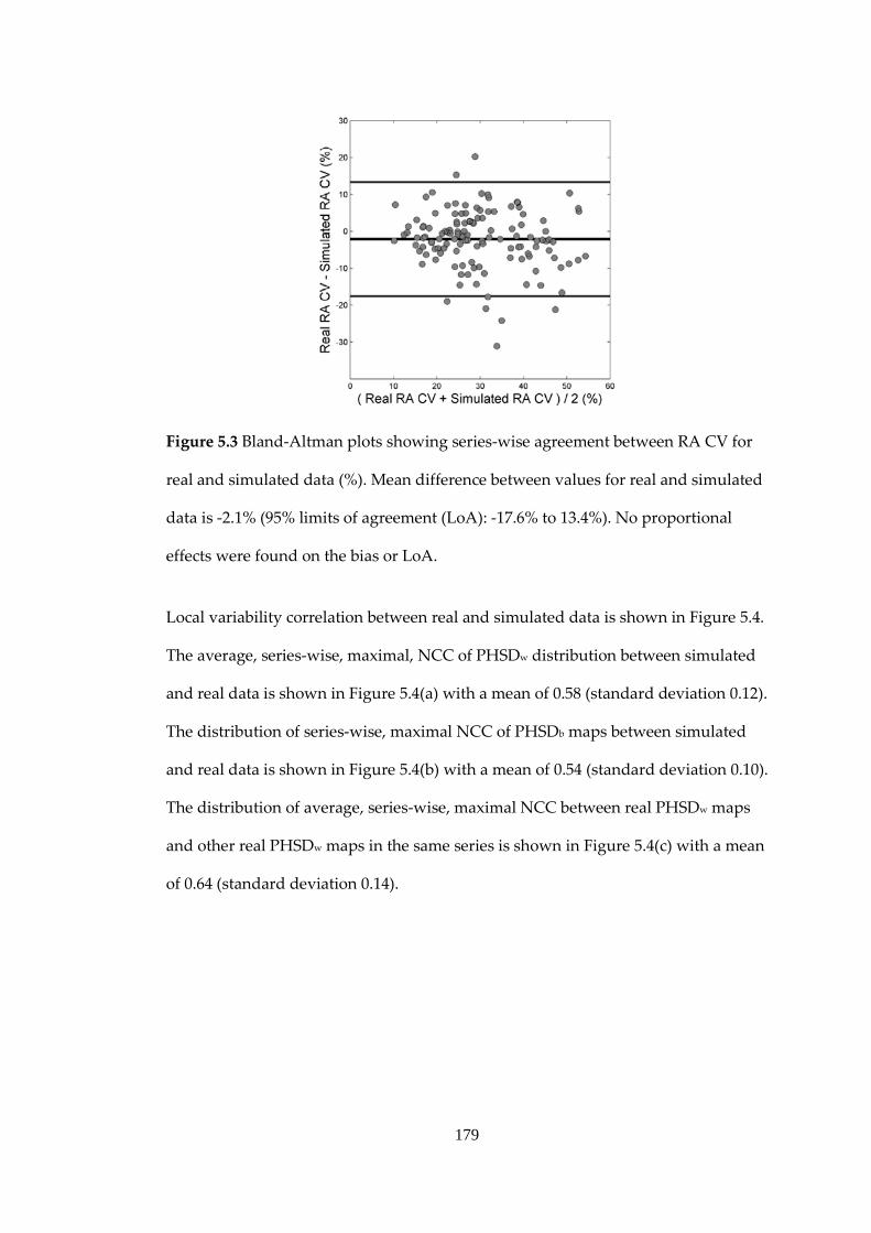
179

Figure 5.3 Bland-Altman plots showing series-wise agreement between RA CV for

real and simulated data (%). Mean difference between values for real and simulated

data is -2.1% (95% limits of agreement (LoA): -17.6% to 13.4%). No proportional

effects were found on the bias or LoA.

Local variability correlation between real and simulated data is shown in Figure 5.4.

The average, series-wise, maximal, NCC of PHSDw distribution between simulated

and real data is shown in Figure 5.4(a) with a mean of 0.58 (standard deviation 0.12).

The distribution of series-wise, maximal NCC of PHSDb maps between simulated

and real data is shown in Figure 5.4(b) with a mean of 0.54 (standard deviation 0.10).

The distribution of average, series-wise, maximal NCC between real PHSDw maps

and other real PHSDw maps in the same series is shown in Figure 5.4(c) with a mean

of 0.64 (standard deviation 0.14).

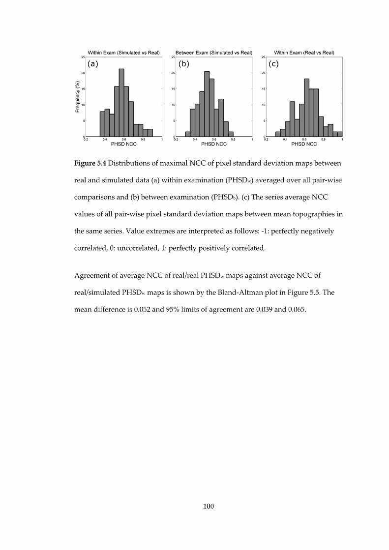
180

Figure 5.4 Distributions of maximal NCC of pixel standard deviation maps between

real and simulated data (a) within examination (PHSDw) averaged over all pair-wise

comparisons and (b) between examination (PHSDb). (c) The series average NCC

values of all pair-wise pixel standard deviation maps between mean topographies in

the same series. Value extremes are interpreted as follows: -1: perfectly negatively

correlated, 0: uncorrelated, 1: perfectly positively correlated.

Agreement of average NCC of real/real PHSDw maps against average NCC of

real/simulated PHSDw maps is shown by the Bland-Altman plot in Figure 5.5. The

mean difference is 0.052 and 95% limits of agreement are 0.039 and 0.065.

181

Figure 5.5 Benchmarking of PHSDw NCC values between real and simulated data:

Bland-Altman plot showing agreement of average NCC for real/real PHSDw map

comparisons and average NCC for real/simulated PHSDw map comparisons. Solid

lines represent a uniform bias of 0.052 and 95% limits of agreement of 0.039 to 0.065.

The dashed line represents the statistically significant linear proportional bias.

Examples of mean reflectance images, mean topographies and corresponding

PHSDw maps for real and simulated data are shown in Figures 5.6 and 5.7.

Examples of series average mean reflectance images, series average mean

topographies and corresponding PHSDb maps for real and simulated data are

shown in Figures 5.8 and 5.9.

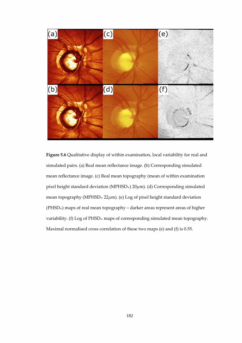
182





mean topography (MPHSDw 22µm). (e) Log of pixel height standard deviation

(PHSDw) maps of real mean topography – darker areas represent areas of higher

variability. (f) Log of PHSDw maps of corresponding simulated mean topography.

Maximal normalised cross correlation of these two maps (e) and (f) is 0.55.

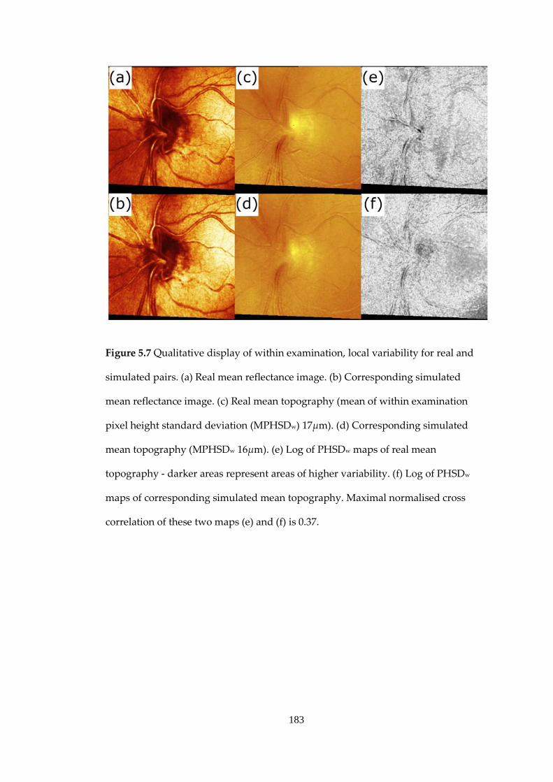
183





mean topography (MPHSDw 16µm). (e) Log of PHSDw maps of real mean

topography - darker areas represent areas of higher variability. (f) Log of PHSDw

maps of corresponding simulated mean topography. Maximal normalised cross

correlation of these two maps (e) and (f) is 0.37.

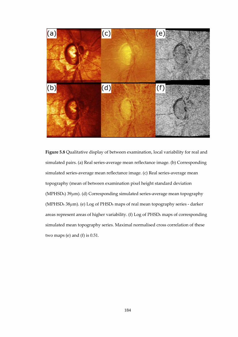
184










185










186

5.3 Discussion

There is no gold-standard method for detecting structural changes in the

glaucomatous eye. One solution might be afforded by simulating series of ONH

measurements with well estimated measurement variability characteristics. This

study proposes a blueprint for such an approach, using images from CSLO

technology. This simulation is based on empirically derived parameters from

previous studies and HRT specifications from published reports. The usefulness of a

simulation is critically dependent on the degree to which it reproduces the

characteristics of real data. The simulation presented in this study reproduces well

both the spatial characteristics, and the magnitude, of variability in short-time series

of HRT data both within examination acquisition and between examinations. Image

correlation of real and simulated spatial variability maps tend to be slightly less

than the correlation of real spatial variability maps with each other, but the

quantitative and qualitative differences are very small. The simulation also

generates realistic values for RA which is a clinically useful parameter for

monitoring change. The contribution simulation can have, independent of, and

before the collection of real data for scientific studies or clinical trials which aim to

assess the validity of change detection measures, cannot be overstated. Given any

number of baseline patient scans, it enables unlimited modification to the length of

series, frequency of testing and variability over time of the data. It also may reduce

potentially wasted cost and time involved in data collection given that study design

may be optimised in advance by testing preliminary hypotheses on simulated test-

bed data.

The simulations were bench-marked against real short-time series. Clinically

significant change is highly unlikely to have taken place during the short study

187

period and age related effects will also be almost non-existent; the only changes in

the series over time will be real fluctuations in the tissue morphology and variability

in the measuring device and settings. This study has used parameters from previous

studies on the movement of the eye (and, as a result, the movement of the ONH)

during fixation from previous studies, along with the reasonable estimates of

operator variability in initial ONH centration and the variability inherent in the

device hardware in an attempt to make these assumptions as realistic as possible.

Errors in estimating these parameters may result in inaccuracies in the simulation.

Other potential sources of variability, such as the ocular pulse and IOP changes,

have not been introduced as they have not been sufficiently well characterised. The

ocular pulse has been shown to contribute to changes in vessel calibre (Chen et al.,

1994, Knudtson et al., 2004) and changes in the backward and forward movements

of the retinal surface in vessel free areas (Chauhan and McCormick, 1995). Long-

term and short-term IOP changes can also cause changes in the vessel calibre (Shin

et al., 1991) along with changes in optic disc cupping (Parrow et al., 1992) and size

(Poostchi et al., 2010). The apparent random parabolic deformation of topographies

over time due to random changes in the distance of the eye from the device between

examinations (known as parabolic error) has been observed to be significant

(Balasubramanian et al., 2011). The simulation does not account for these effects but

it might be possible to do so using appropriate parameters. Despite these potential

shortcomings, the simulations appear to realistically reproduce observed

topographic variability.

Previous attempts to simulate series of ONH or retinal images are few and far

between. One approach involved simulating retardance image series obtained from

SLP baseline images (Vermeer et al., 2006). SLP differs from CSLT in that it

measures relevant anatomy in a different manner, and has different sources of

188

variability. Another simulation methodology, specific to HRT data, has used small

misalignments of identical finalised or post-processed single topographies to

generate longitudinal series (Patterson et al., 2005). This approach formed the basis

of the simulation used in Chapter 4 to investigate MPHSD. Although it reproduces

some of the global variability inherent in no-change patient HRT data, by design it

cannot reproduces the spatial and feature dependent variability involved in

topography fitting and topography alignment. It is also unsatisfactory from a

theoretical point of view as it is difficult to estimate the relationship of acquisition

noise factors and the variability of post-processed topographies. The methodology

presented in this study contrasts by using all the three-dimensional information

acquired in the HRT scan. Further, a key component of the simulation described in

the current study is that the simulated scans are re-imported into the HRT III

software. Thus any misalignments added both within examination and between

examination will be subject to partial correction by the HRT III alignment

algorithms. This is consistent with the procedure for real patient data.

Although within examination single topographies are more closely related than

between session topographies, because of the effects of between examination

repositioning of the patient and re-alignment of the scanner to the eye/ONH, the

simulation assumes no auto-correlation in time (knowing one value does not

provide you with any information of another value) between examinations. Also,

the within examination noise parameters do not change with time nor do the

differences between examinations. These assumptions are justified on the basis of

study results showing no difference in variability between scans with intervals

varying from 1 hour to 4 weeks (Chauhan and MacDonald, 1995).

189

There are a few cases of variability being poorly reproduced in simulated series as

can be seen in Figure 5.2(a). Here, the largest anomalies are above the line of

agreement showing that, in these cases, the average, global within mean topography

variability is higher in the simulation than in real series. This may indicate that the

optical section stack used to seed the simulation has more motion noise or lower

image quality than those in the rest of the real series. Although the simulation

model presented here will allow some alignment before noise addition, it is never

possible to attain a motion-free, noise-free image stack. Thus the simulation

depends on the optical section stack selected to seed each simulated series. Apart

from random differences in a small sample of 5 mean topographies, there may be

other potential causes for discrepancies in reproducing the variability of real data,

for example, some differences in RA variability may be due to small differences in

contour line placement between the real and simulated baseline topographies.

Windowing, as stated in the methodology may have small systematic effects on

differences in the calculations of variability between real and simulated data due to

the potential null values on optical section and topography image edges. However,

windowing caused by axial shifts should not affect the topography formation

process as any missing data will be in the low intensity “tails” of each axial intensity

profile. Topographic height information is mostly derived from the central

maximum of each axial intensity profile. Vertical axis shifts have the potential to

most affect the topography formation. Despite this, between examination, vertical

translations of scan triplets greater than 20 pixels between scans resulting in the loss

of more than 20 pixels at the top or bottom of a mean topography will occur in

approximately only 5% of simulated follow-up examinations and furthermore have

only a small effect on the alignment algorithms of the HRT and the calculation of

variability values.

190

The simulation makes the simplifying assumption that eye movement and

measurement noise parameters are the same for all patients. This assumption

seemed sufficient in reproducing many of the characteristics of real data.

Furthermore, it is important to note that in real patient data, patients with varying

degrees of lens opacity were scanned. This allowed the effects of a wide range of

image quality to be modelled, with some eyes having high within and between

examination variability. That this is also observed in the simulated data suggests

that much of the observed range of image variability is a consequence of the range

in the quality of ocular media and the structure of the ONHs themselves.

Future work could usefully consider the formation process in the CSLO pixels

(Gruppetta, 2009), allowing the modelling of other processes which occur before the

summation of light at the detector for each pixel by modifying the PSF during and

between acquisition sessions. These include changes in pupil diameter, media

opacities and changes in uncorrected lower order aberrations (defocus and

astigmatism). This simulation provides a model to test progression algorithm

specificity appropriate to the baseline image quality, but cannot mimic

systematically changing image quality over time. The long-term changes in the

optical quality of the eye over time (increased scatter and absorption) resulting in a

reduced and noisier light signal reflected to the device detector will need to be

addressed in order to mimic this feature in some topographic series over time.

The introduction in the simulations of topographic changes associated with focal

and diffuse glaucomatous damage in the ONH need to be investigated. By adding

change to a series of replicate HRT scans, and then overlaying measurement noise

from this simulation, the sensitivity of change detection algorithms may be assessed

191

(as the underlying location, temporal sequence and magnitude of the superimposed

change is known).

A stable series of measurements can be generated by simply adding random noise.

Such series may also be used to test specificity of statistical change detection

algorithms developed for detecting progression. However, in reality, there are many

other sources of variability in ONH scans such as eye movements, head movements

and device noise, the effects of which may be falsely detected as true morphological

change by these techniques. Such variability is manifestly more complex than

simple, additive noise and therefore a more realistic stable series simulation is

needed to more accurately test the specificity of these algorithms. Stability in any

clinical series of data is uncertain, whereas in a modelled series it is certain.

So, in conclusion, the methodology outlined in this work has definite use in

producing benchmark data on which the false positive rates of statistical methods

for detecting HRT progression can be examined. This could also improve the

confidence of change detected by these techniques in clinical studies. Simulating

series of progressive change in HRT series awaits further investigation. Still, the

results of this study are presented as a proof of principle for a solution towards the

seemingly intractable problem of developing reliable methods for detecting disease

progression in glaucoma.

192

6. Conclusion and Further Work

As continued research expands, modern knowledge of the various factors

characterising glaucomatous ONH progression will undoubtedly change. The

objectives of this thesis are to assess progression detection algorithms in ONH data

from CLST technology, specifically the HRT. The key findings in the sections of this

thesis are as follows.

Chapter 2 compares optic disc changes using automated analyses of HRT images

with assessments, by glaucoma specialists, of change in stereoscopic photographs.

Different statistical methods for detecting structural changes in HRT images exhibit

only moderate agreement with each other and have poor agreement with expert-

assessed change in optic disc stereophotographs. Because it is undermined by

limitations in the specificity and between-observer agreement, the use of optic disc

photograph assessment alone as a reference standard is not helpful in determining

the optimal automated change detection algorithm in series of HRT images.

Chapter 3 examines the effects of measurement variability across a range of

characteristics on the performance of some basic univariate statistical techniques to

detect underlying trends. This work demonstrates that serial autocorrelation of

measurement error can have large detrimental effects on the statistical power to

detect change in these methods even when the measurement noise is low. Of the

methods investigated, similar powers are observed on average across a range of

measurement noise characteristics – but non-parametric, rank-based methods offer

the advantage of not depending on linear change over time and may be preferable

for progression detection.

193

Chapter 4 finds quality metrics of HRT images to be highly predictive of within

examination pixel-wise measurement variability – measured by the MPHSD. A

simple simulation is used to demonstrate that uniform levels of misalignment noise

applied to different ONH images before image averaging can produce a wide range

of MPHSD values. This indicates the dependence of MPHSD on the ONH

morphology itself. Subjective assessment of image quality of HRT data exhibits a

low between-observer agreement but averaged panel scores have good agreement

with MPHSD values. The average MPHSD across a series of HRT images variability

is a strong predictor of series RA variability but for an individual examination

MPHSD was not predictive of the reliability of the RA measurement. This indicates

that MPHSD may not be a useful way to weight individual examination

information.

Chapter 5 describes how a novel simulation propagates HRT pseudo-longitudinal

series from the three-dimensional data of a single baseline scan. The simulation is

implemented using empirical and theoretical measurement noise parameters. This

approach is validated by its ability to reproduce the variability of CLST data both on

a local and global scale of the ONH. This means it can provide a test-bed to evaluate

the specificity and sensitivity of CSLT progression detection algorithms.

In summary, the new contributions to the field of imaging in glaucoma are:

- establishing that methods such as using expert assessed ONH

stereophotographs as reference standards for glaucomatous change do not

provide useful insights on how well or badly HRT glaucoma progression

algorithms perform

194

- demonstrating considerable disagreement between current HRT

progression detection algorithms motivating a continued search for an

optimum technique

- characterising the strong relationships of image quality and morphological

characteristics with HRT measurement variability

- emphasising the detrimental effects of measurement autocorrelation on the

ability to detect statistically significant trends in RA data

- the development of a novel and empirically based simulation which can

reproduce virtual HRT data with variability similar in magnitudes and

spatial characteristics to real data and thus address these issues

Following these findings, future work could usefully consider:

- discovering predictors of the noisy measurements in HRT imaging and in

other imaging modalities

- modelling change in the developed simulation of longitudinal HRT image

series

- application of the simulation methodology developed in this thesis to other

imaging modalities

- investigate the advantages of rank-based over parametric-based trend

detection techniques for non-linear models of change

- devising change detection algorithms for HRT and newer imaging

modalities based on these conclusions and testing these on simulated and

real data

195

APPENDIX A: Linear

Regression Permuted Test

Statistics

The univariate OLS linear regression solution considers the problem of fitting 𝑛

observed data points (𝑥𝑖 ,𝑦𝑖) for independent variable 𝑥 and dependent variable 𝑦

to a straight-line model:

𝒚(𝒙) = 𝒚(𝒙; 𝛼,𝛽) = 𝛼 + 𝛽𝒙+ 𝜺

where 𝛼 is the predicted value of 𝑦 when 𝑥=0 and 𝛽 describes the estimated linear

trend of 𝑦 with changing 𝑥. The measurement errors 𝜀𝑖 at each point are denoted

by 𝜺. OLS linear regression derives a solution to this model by searching for the

parameters 𝛼 and 𝛽 which minimise the measurement errors 𝜀𝑖. From this solution,

a test statistic can be derived from which the statistical significance of the slope of

fitted line 𝛽 can be inferred. The following analysis examines the effect of

reordering while using a permutation test on this test statistic. The estimate 𝛽 and

its standard error 𝑠𝛽 are defined by

𝛽 = �𝑛𝑆𝑥𝑦 − 𝑆𝑥𝑆𝑦𝑛𝑆𝑥𝑥 − 𝑆𝑥2

�,

196

𝑠𝛽 = �𝑛𝑠𝜀

𝑛𝑆𝑥𝑥 − 𝑆𝑥2,

where

𝑠𝜀 = 𝑛𝑆𝑦𝑦 − 𝑆𝑦2 − 𝛽2�𝑛𝑆𝑥𝑥 − 𝑆𝑥2�

and 𝑆𝑥 = ∑ 𝑥𝑖𝑛𝑖=1 , 𝑆𝑦 = ∑ 𝑦𝑖𝑛

𝑖=1 , 𝑆𝑥𝑥 = ∑ 𝑥𝑖2𝑛𝑖=1 , 𝑆𝑦𝑦 = ∑ 𝑦𝑖2𝑛

𝑖=1 , 𝑆𝑥𝑦 =

∑ 𝑥𝑖𝑦𝑖𝑛𝑖=1 are the OLS linear regression coefficients.

In the paradigm of a permutation test, 𝑥𝑖 are randomly re-ordered while fixing the

order of 𝑦𝑖. Thus during a permutation test, 𝑛, 𝑆𝑥, 𝑆𝑦, 𝑆𝑥𝑥, 𝑆𝑦𝑦 are fixed. It is

possible to compare the ranking effects from re-ordering on 𝛽 and 𝑠𝛽 by treating

these as constants during permutation. The slope test statistic from OLS linear

regression is then:

𝛽𝑆𝛽

=𝛽

�𝑛𝑠𝜀2

�𝑛𝑆𝑥𝑥 − 𝑆𝑥2�

=𝛽

�𝑛 �𝑛𝑆𝑦𝑦 − 𝑆𝑦2 − 𝛽�𝑛𝑆𝑥𝑥 − 𝑆𝑥2�

𝑛 − 2 �

�𝑛𝑆𝑥𝑥 − 𝑆𝑥2�

=𝛽

�𝐶1 − 𝛽𝐶2

= 𝑓(𝛽)

where:

197

𝐶1 =�𝑛2𝑆𝑦𝑦 − 𝑛𝑆𝑦2�

(𝑛 − 2)�𝑛𝑆𝑥𝑥 − 𝑆𝑥2�,

𝐶2 =�𝑛2𝑆𝑥𝑥 − 𝑛𝑆𝑥2�

(𝑛 − 2)�𝑛𝑆𝑥𝑥 − 𝑆𝑥2�

are invariant throughout permutation. For a real, meaningful (𝑛 > 2) solution of the

test-statistic 𝛽𝑆𝛽

, the denominator must yield:

𝐶1 − 𝛽𝐶2 > 0.

Thus during a permutation test the test statistic 𝑓(𝛽) is a monotonic (order-

preserving) function of 𝛽. Stated formally, this requires for any 𝑗𝑡ℎ and 𝑘𝑡ℎ

permutations given

𝛽𝑘 > 𝛽𝑗

that

𝑓(𝛽𝑘) > 𝑓�𝛽𝑗�.

This means that the order the resulting test-statistic from each permutation 𝛽𝑆𝛽

will

be unchanged relative to the respective 𝛽 for that permutation.

198

APPENDIX B – Image

Transformation Details

The affine transformation (a linear transformation with translation) of a set of 𝑖

points in three-dimensional space with coordinates (𝑥𝑖 ,𝑦𝑖 , 𝑧𝑖) to a point with new

coordinates (𝑥𝑖′,𝑦𝑖′, 𝑧𝑖′) can be represented by matrix algebra. When considering

only rotation, shear, scaling and translation or shift, each can be given by the

following affine transformation matrices using homogeneous coordinates:

Translation along 𝑥, 𝑦, 𝑧 axes by displacements 𝑡𝑥, 𝑡𝑦 and 𝑡𝑧:

�

𝑥𝑖′𝑦𝑖′𝑧𝑖′1

� = �

1 0 0 00 1 0 00 0 1 0𝑡𝑥 𝑡𝑦 𝑡𝑧 1

� � �

𝑥𝑖𝑦𝑖𝑧𝑖1

� � , 𝒑′ = T𝒑

Rotation about 𝑧 axis by angle 𝜃:

�


� = �

cos𝜃 − sin𝜃 0 0sin 𝜃 cos𝜃 0 0

0 0 1 00 0 0 1

� � �


� � , 𝒑′ = R𝑧𝒑

Rotation about 𝑥 axis by angle ∅:

�


� = �

1 0 0 00 cos∅ − sin∅ 00 sin∅ cos∅ 00 0 0 1

� � �


� � , 𝒑′ = R𝑥𝒑

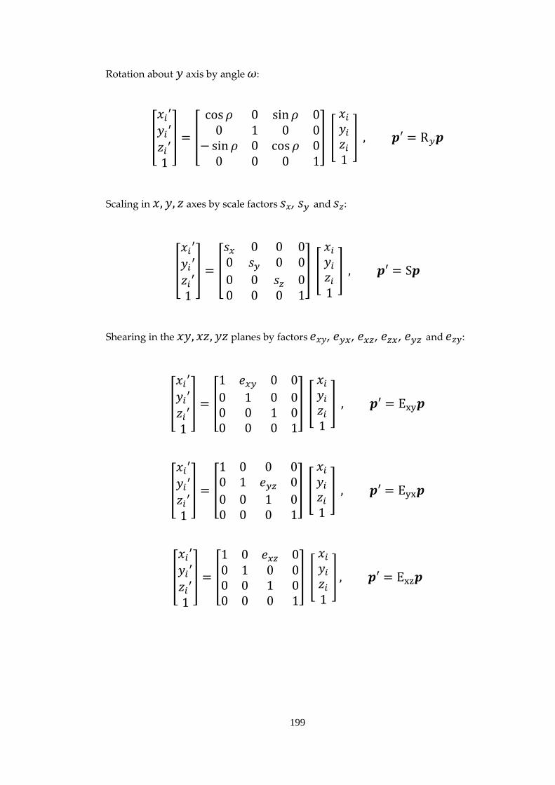
199

Rotation about 𝑦 axis by angle 𝜔:

�


� = �

cos𝜌 0 sin𝜌 00 1 0 0

− sin𝜌 0 cos𝜌 00 0 0 1

� ��


� � , 𝒑′ = R𝑦𝒑

Scaling in 𝑥,𝑦, 𝑧 axes by scale factors 𝑠𝑥, 𝑠𝑦 and 𝑠𝑧:

�


� = �

𝑠𝑥 0 0 00 𝑠𝑦 0 00 0 𝑠𝑧 00 0 0 1

� � �


� � , 𝒑′ = S𝒑

Shearing in the 𝑥𝑦, 𝑥𝑧,𝑦𝑧 planes by factors 𝑒𝑥𝑦, 𝑒𝑦𝑥, 𝑒𝑥𝑧, 𝑒𝑧𝑥, 𝑒𝑦𝑧 and 𝑒𝑧𝑦:

�


� = �

1 𝑒𝑥𝑦 0 00 1 0 00 0 1 00 0 0 1

� � �


� � , 𝒑′ = Exy𝒑

�


� = �

1 0 0 00 1 𝑒𝑦𝑧 00 0 1 00 0 0 1

� � �


� � , 𝒑′ = Eyx𝒑

�


� = �

1 0 𝑒𝑥𝑧 00 1 0 00 0 1 00 0 0 1

� � �


�� , 𝒑′ = Exz𝒑

200

�


� = �

1 0 0 00 1 0 0𝑒𝑧𝑥 0 1 00 0 0 1

� � �


� � , 𝒑′ = Ezx𝒑

�


� = �

1 0 0 00 1 𝑒𝑦𝑧 00 0 1 00 0 0 1

� � �


� � , 𝒑′ = Eyz𝒑

�


� = �

1 0 0 00 1 0 00 𝑒𝑧𝑦 1 00 0 0 1

� � �


� � , 𝒑′ = Ezy𝒑

Finally all transformations can be combined with the new coordinates 𝒑′ depending

on the ordering of each transformation. An example below would represent image

coordinates being transformed first, then rotated about the 𝑧, 𝑥,𝑦 axes then scaled

and finally sheared:

𝒑′ = ExyEyxExzEzxEyzEzy S R𝑦R𝑥R𝑧T𝒑

In designing the simulation for HRT mean topography generation, the probability

distributions for all the required parameters are chosen from the following random

distributions:

𝑡𝑥~𝑁 �0,𝑊

256𝑝� , 𝑡𝑦~𝑁�0,𝑊

256𝑝� , 𝑡𝑧~𝑁(0,10𝜇𝑚 )

𝜃~𝑁(0°, 0.25°), ∅~𝑁(0°, 0.1°), 𝜌~𝑁(0°, 0.1°)

𝑠𝑥~𝑁�0,𝑊10� , 𝑠𝑦~𝑁�0,

𝑊10� , 𝑠𝑧~𝑁�0 ,

𝑊10�

201

𝑒𝑥𝑦~𝑁(0,10), 𝑒𝑥𝑦~𝑁(0,10)

𝑒𝑥𝑦~𝑁(0,10), 𝑒𝑥𝑦~𝑁(0,10)

𝑒𝑥𝑦~𝑁(0,10), 𝑒𝑥𝑦~𝑁(0,10)

where 𝑊 is the width and height of the square image in pixels and 𝑝 is the unit of

one pixel width. Where no units are indicated, parameters are dimensionless ratios.

Transformations are applied at a sub-pixel level, using a bilinear interpolation

algorithm.

202

7. Bibliography

ABRAMS, L. S., SCOTT, I. U., SPAETH, G. L., QUIGLEY, H. A. & VARMA, R. 1994. Agreement among optometrists, ophthalmologists, and residents in evaluating the optic disc for glaucoma. Ophthalmology, 101, 1662-7.

ADVANCED GLAUCOMA INTERVENTION STUDY INVESTIGATORS 2000. The advanced glaucoma intervention study (AGIS): 7. The relationship between control of intraocular pressure and visual field deterioration. Am J Ophthalmol, 130, 429-40.

AIRAKSINEN, P. J. & DRANCE, S. M. 1985. Neuroretinal rim area and retinal nerve fiber layer in glaucoma. Arch Ophthalmol, 103, 203-204.

ALLINGHAM, R. R. & SHIELDS, M. B. 2005. Shields' textbook of glaucoma, Philadelphia, Lippincott Willliams & Wilkins.

ALTANGEREL, U., SPAETH, G. L. & STEINMANN, W. C. 2006. Assessment of function related to vision (AFREV). Ophthalmic Epidemiol, 13, 67-80.

ALTMAN, D. G. 1999. Practical statistics for medical research, Boca Raton, Fla., Chapman & Hall/CRC.

ALTMAN, D. G. & BLAND, J. M. 1994. Diagnostic tests 3: receiver operating characteristic plots. BMJ, 309, 188.

AMERICAN ACADEMY OF OPHTHALMOLOGY GLAUCOMA PANEL 2010. Primary Open-Angle Glaucoma. Preferred Practice Pattern Guidelines. San Francisco, CA.

ARMALY, M. F. 1968. Genetic factors related to glaucoma. Ann N Y Acad Sci, 151, 861-75.

ARNDT, S., CIZADLO, T., ANDREASEN, N. C., HECKEL, D., GOLD, S. & O'LEARY, D. S. 1996. Tests for comparing images based on randomization and permutation methods. J Cereb Blood Flow Metab, 16, 1271-9.

ARTES, P. H. & CHAUHAN, B. C. 2005. Longitudinal changes in the visual field and optic disc in glaucoma. Prog Retin Eye Res, 24, 333-54.

ARTES, P. H. & CRABB, D. P. 2010. Estimating normative limits of Heidelberg Retina Tomograph optic disc rim area with quantile regression. Invest Ophthalmol Vis Sci, 51, 355-61.

203

ASAOKA, R., STROUTHIDIS, N. G., KAPPOU, V., GARDINER, S. K. & GARWAY-HEATH, D. F. 2009. HRT-3 Moorfields reference plane: effect on rim area repeatability and identification of progression. British Journal of Ophthalmology, 93, 1510-1513.

ASAWAPHUREEKORN, S., ZANGWILL, L. & WEINREB, R. N. 1996. Ranked-segment distribution curve for interpretation of optic nerve topography. J Glaucoma, 5, 79-90.

AZUARA-BLANCO, A., KATZ, L. J., SPAETH, G. L., VERNON, S. A., SPENCER, F. & LANZL, I. M. 2003. Clinical agreement among glaucoma experts in the detection of glaucomatous changes of the optic disk using simultaneous stereoscopic photographs. American journal of ophthalmology, 136, 949-950.

BALASUBRAMANIAN, M., BOWD, C., VIZZERI, G., WEINREB, R. N. & ZANGWILL, L. M. 2009. Effect of image quality on tissue thickness measurements obtained with spectral domain-optical coherence tomography. Opt Express, 17, 4019-36.

BALASUBRAMANIAN, M., BOWD, C., WEINREB, R. N. & ZANGWILL, L. M. 2011. Agreement between Heidelberg Retina Tomograph-I and -II in detecting glaucomatous changes using topographic change analysis. Eye, Published ahead of print.

BALAZSI, A. G., DRANCE, S. M., SCHULZER, M. & DOUGLAS, G. R. 1984. Neuroretinal rim area in suspected glaucoma and early chronic open-angle glaucoma. Correlation with parameters of visual function. Arch Ophthalmol, 102, 1011-1014.

BARNDORFF-NIELSEN, O. 1977. Exponentially Decreasing Distributions for the Logarithm of Particle Size. Proceedings of the Royal Society of London. Series A, Mathematical and Physical Sciences, 353, 401-419.

BARRY, C. J., YOGESAN, K., JITSKAIA, L., MORGAN, W. H., HOUSE, P. H. & EIKELBOOM, R. H. 1998. A personal computer-based method of stereo chronometry for measuring neuroretinal rim width: a pilot study. Aust N Z J Ophthalmol, 26 Suppl 1, S22-5.

BARTLING, H., WANGER, P. & MARTIN, L. 2009. Automated quality evaluation of digital fundus photographs. Acta Ophthalmol, 87, 643-7.

BARTSCH, D. U. & FREEMAN, W. R. 1993. Laser-Tissue Interaction and Artifacts in Confocal Scanning Laser Ophthalmoscopy and Tomography. Neuroscience & Biobehavioral Reviews, 17, 459-467.

BATHIJA, R., ZANGWILL, L., BERRY, C. C., SAMPLE, P. A. & WEINREB, R. N. 1998. Detection of early glaucomatous structural damage with confocal scanning laser tomography. J Glaucoma, 7, 121-7.

204

BECKER, B., KOLKER, A. E. & ROTH, F. D. 1960. Glaucoma family study. Am J Ophthalmol, 50, 557-67.

BELLEZZA, A. J., RINTALAN, C. J., THOMPSON, H. W., DOWNS, J. C., HART, R. T. & BURGOYNE, C. F. 2003. Deformation of the lamina cribrosa and anterior scleral canal wall in early experimental glaucoma. Invest Ophthalmol Vis Sci, 44, 623-37.

BENGTSSON, B., OLSSON, J., HEIJL, A. & ROOTZEN, H. 1997. A new generation of algorithms for computerized threshold perimetry, SITA. Acta Ophthalmol Scand, 75, 368-75.

BERGIN, C., GARWAY-HEATH, D. F. & CRABB, D. P. 2008. Evaluating the effect of the new alignment algorithm for longitudinal series of Heidelberg retina tomography images. Acta Ophthalmol, 86, 207-14.

BEYERSDORFF, D., TAYMOORIAN, K., KNOSEL, T., SCHNORR, D., FELIX, R., HAMM, B. & BRUHN, H. 2005. MRI of Prostate Cancer at 1.5 and 3.0 T: Comparison of Image Quality in Tumor Detection and Staging. Am. J. Roentgenol., 185, 1214-1220.

BLAND, J. M. & ALTMAN, D. G. 1986. Statistical methods for assessing agreement between two methods of clinical measurement. Lancet, 1, 307-10.

BOVIK, A. C. 2009. The essential guide to video processing, Amsterdam ; Boston, Academic Press/Elsevier.

BOWD, C., BALASUBRAMANIAN, M., WEINREB, R. N., VIZZERI, G., ALENCAR, L. M., O'LEARY, N., SAMPLE, P. A. & ZANGWILL, L. M. 2009. Performance of Confocal Scanning Laser Tomograph Topographic Change Analysis (TCA) for Assessing Glaucomatous Progression. Invest. Ophthalmol. Vis. Sci., 50, 691-701.

BRETT, M., PENNY, W. D. & KIEBEL, S. J. 2003. Introduction to random field theory. In: ASHBURNER, J., FRISTON, K. & PENNY, W. D. (eds.) Human Brain Function. 2nd ed.: Academic Press.

BREUSEGEM, C., FIEUWS, S., STALMANS, I. & ZEYEN, T. Variability of the Standard Reference Height and its Influence on the Stereometric Parameters of the Heidelberg Retina Tomograph 3. Invest Ophthalmol Vis Sci, In press.

BRIGATTI, L. & CAPRIOLI, J. 1995. Correlation of visual field with scanning confocal laser optic disc measurements in glaucoma [published erratum appears in Arch Ophthalmol 1996 Apr;114(4):424]. Arch Ophthalmol, 113, 1191-4.

BRIGATTI, L., WEITZMAN, M. & CAPRIOLI, J. 1995. Regional test-retest variability of confocal scanning laser tomography. Am J Ophthalmol, 120, 433-440.

205

BUDENZ, D. L., CHANG, R. T., HUANG, X., KNIGHTON, R. W. & TIELSCH, J. M. 2005. Reproducibility of retinal nerve fiber thickness measurements using the stratus OCT in normal and glaucomatous eyes. Invest Ophthalmol Vis Sci, 46, 2440-3.

BULLMORE, E. T., SUCKLING, J., OVERMEYER, S., RABE-HESKETH, S., TAYLOR, E. & BRAMMER, M. J. 1999. Global, voxel, and cluster tests, by theory and permutation, for a difference between two groups of structural MR images of the brain. IEEE Trans Med Imaging, 18, 32-42.

BURGANSKY-ELIASH, Z., WOLLSTEIN, G., BILONICK, R. A., ISHIKAWA, H., KAGEMANN, L. & SCHUMAN, J. S. 2007. Glaucoma detection with the Heidelberg Retina Tomograph 3. Ophthalmology, 114, 466-71.

BURK, R. O., VIHANNINJOKI, K., BARTKE, T., TUULONEN, A., AIRAKSINEN, P. J., VOLCKER, H. E. & KONIG, J. M. 2000. Development of the standard reference plane for the Heidelberg retina tomograph. Graefes Arch Clin Exp Ophthalmol, 238, 375-84.

BURK, R. O. W., ROHRSCHNEIDER, K., VOLCKER, H. E. & ZINSER, G. 1990. Analysis of three-dimentional optic disk topography by laser scanning tomography. Parameter definition and evaluation of parameter inter-dependence. In: NASEMANN, J. & BURK, R. (eds.) Scanning Laser Ophthalmoscopy and Tomography. Munchen: Quintessenz.

BURR, J., AZUARA-BLANCO, A. & AVENELL, A. 2005. Medical versus surgical interventions for open angle glaucoma. Cochrane Database Syst Rev, CD004399.

CAPEL, D. 2004. Image mosaicing and super-resolution, London ; New York, Springer.

CHANG, R. T., KNIGHT, O. J., FEUER, W. J. & BUDENZ, D. L. 2009. Sensitivity and specificity of time-domain versus spectral-domain optical coherence tomography in diagnosing early to moderate glaucoma. Ophthalmology, 116, 2294-9.

CHAUHAN, B. C., BLANCHARD, J. W., HAMILTON, D. C. & LEBLANC, R. P. 2000. Technique for detecting serial topographic changes in the optic disc and peripapillary retina using scanning laser tomography. Invest Ophthalmol Vis Sci, 41, 775-82.

CHAUHAN, B. C., GARWAY-HEATH, D. F., GONI, F. J., ROSSETTI, L., BENGTSSON, B., VISWANATHAN, A. C. & HEIJL, A. 2008. Practical recommendations for measuring rates of visual field change in glaucoma. Br J Ophthalmol, 92, 569-73.

CHAUHAN, B. C., HUTCHISON, D. M., ARTES, P. H., CAPRIOLI, J., JONAS, J. B., LEBLANC, R. P. & NICOLELA, M. T. 2009. Optic Disc Progression in

206

Glaucoma: Comparison of Confocal Scanning Laser Tomography to Optic Disc Photographs in a Prospective Study. Invest. Ophthalmol. Vis. Sci., 50, 1682-1691.

CHAUHAN, B. C., LEBLANC, R. P., MCCORMICK, T. A. & ROGERS, J. B. 1994. Test-retest variability of topographic measurements with confocal scanning laser tomography in patients with glaucoma and control subjects. Am J Ophthalmol, 118, 9-15.

CHAUHAN, B. C. & MACDONALD, C. A. 1995. Influence of Time Separation on Variability Estimates of Topographic Measurements with Confocal Scanning Laser Tomography. Journal of Glaucoma, 4, 189-193.

CHAUHAN, B. C. & MCCORMICK, T. A. 1995. Effect of the cardiac cycle on topographic measurements using confocal scanning laser tomography. Graefes Archive for Clinical & Experimental Ophthalmology.

CHAUHAN, B. C., MCCORMICK, T. A., NICOLELA, M. T. & LEBLANC, R. P. 2001. Optic disc and visual field changes in a prospective longitudinal study of patients with glaucoma: comparison of scanning laser tomography with conventional perimetry and optic disc photography. Arch Ophthalmol, 119, 1492-9.

CHEN, H. C., PATEL, V., WIEK, J., RASSAM, S. M. & KOHNER, E. M. 1994. Vessel diameter changes during the cardiac cycle. Eye, 8 ( Pt 1), 97-103.

CHYLACK, L. T., JR., WOLFE, J. K., SINGER, D. M., LESKE, M. C., BULLIMORE, M. A., BAILEY, I. L., FRIEND, J., MCCARTHY, D. & WU, S. Y. 1993. The Lens Opacities Classification System III. The Longitudinal Study of Cataract Study Group. Arch Ophthalmol, 111, 831-6.

CIOFFI, G. A., ROBIN, A. L., EASTMAN, R. D., PERELL, H. F., SARFARAZI, F. A. & KELMAN, S. E. 1993. Confocal laser scanning ophthalmoscope. Reproducibility of optic nerve head topographic measurements with the confocal laser scanning ophthalmoscope. Ophthalmology, 100, 57-62.

CIULLA, T., REGILLO, C. & HARRIS, A. 2003. Retina and Optic Nerve Imaging,, Philadelphia, Lippincott Williams and Wilkins.

COFFEY, M., REIDY, A., WORMALD, R. P. L., WU, J. X., WRIGHT, L. A. & COURTNEY, P. 1993. Prevalence of glaucoma in the west of Ireland. Br J Ophthalmol, 77, 17-21.

COHEN, J. 1988. Statistical power analysis for the behavioral sciences, Hillsdale, N.J., L. Erlbaum Associates.

COLEMAN, A. L., SOMMER, A., ENGER, C., KNOPF, H. L., STAMPER, R. L. & MINCKLER, D. S. 1996. Interobserver and Intraobserver Variability in the

207

Detection of Glaucomatous Progression of the Optic Disc. Journal of Glaucoma, 5, 384-389.

COLLINS, D. L., ZIJDENBOS, A. P., KOLLOKIAN, V., SLED, J. G., KABANI, N. J., HOLMES, C. J. & EVANS, A. C. 1998. Design and construction of a realistic digital brain phantom. IEEE Trans Med Imaging, 17, 463-8.

COLTON, T. & EDERER, F. 1980. The distribution of intraocular pressures in the general population. Surv Ophthalmol, 25, 123-9.

COOPS, A., HENSON, D. B., KWARTZ, A. J. & ARTES, P. H. 2006. Automated analysis of heidelberg retina tomograph optic disc images by glaucoma probability score. Invest Ophthalmol Vis Sci, 47, 5348-55.

CRAWFORD, M. L., HARWERTH, R. S., SMITH, E. L., 3RD, SHEN, F. & CARTER-DAWSON, L. 2000. Glaucoma in primates: cytochrome oxidase reactivity in parvo- and magnocellular pathways. Invest Ophthalmol Vis Sci, 41, 1791-802.

CREMER, C. & CREMER, T. 1978. Considerations on a laser-scanning-microscope with high resolution and depth of field. Microsc Acta, 81, 31-44.

CRUM, W. R., HARTKENS, T. & HILL, D. L. G. 2004. Non-rigid image registration: theory and practice. Br J Radiol, 77, S140-153.

DENNISS, J., ECHENDU, D., HENSON, D. B. & ARTES, P. H. 2011. Discus: investigating subjective judgment of optic disc damage. Optom Vis Sci, 88, E93-101.

DETRY-MOREL, M. 2006. Side effects of glaucoma medications. Bull Soc Belge Ophtalmol, 27-40.

DIELEMANS, I., VINGERLING, J. R., WOLFS, R. C., HOFMAN, A., GROBBEE, D. E. & DE JONG, P. T. 1994. The prevalence of primary open-angle glaucoma in a population-based study in The Netherlands. The Rotterdam Study. Ophthalmology, 101, 1851-5.

DODGE, Y. 2008. The concise encyclopedia of statistics, New York, Springer.

DRANCE, S. M. 1989. Disc hemorrhages in the glaucomas. Surv Ophthalmol, 33, 331-7.

DREHER, A. W. & REITER, K. 1992. Scanning laser polarimetry of the retinal nerve fiber layer. SPIE, 1746, 34-41.

DREHER, A. W., TSO, P. C. & WEINREB, R. N. 1991. Reproducibility of topographic measurements of the normal and glaucomatous optic nerve head with the laser tomographic scanner. Am J Ophthalmol, 111, 221-229.

208

DREHER, A. W. & WEINREB, R. N. 1991. Accuracy of Topographic Measurements in a Model Eye with the Laser Tomographic Scanner. Investigative Ophthalmology & Visual Science, 32, 2992-2996.

DRUMMOND, J. C., BRANN, C. A., PERKINS, D. E. & WOLFE, D. E. 1991. A comparison of median frequency, spectral edge frequency, a frequency band power ratio, total power, and dominance shift in the determination of depth of anesthesia. Acta Anaesthesiol Scand, 35, 693-9.

EBERLEIN, E. & KELLER, U. 1995. Hyperbolic Distributions in Finance. Bernoulli, 1, 281-299.

EGAN, J. P. 1975. Signal detection theory and ROC-analysis, New York, Academic Press.

ENGBERT, R. & MERGENTHALER, K. 2006. Microsaccades are triggered by low retinal image slip. Proceedings of the National Academy of Sciences, 103, 7192-7197.

ERVIN, J. C., LEMIJ, H. G., MILLS, R. P., QUIGLEY, H. A., THOMPSON, H. W. & BURGOYNE, C. F. 2002. Clinician change detection viewing longitudinal stereophotographs compared to confocal scanning laser tomography in the LSU Experimental Glaucoma (LEG) Study. Ophthalmology, 109, 467-81.

ESKICIOGLU, A. M. & FISHER, P. S. 1995. Image quality measures and their performance. Communications, IEEE Transactions on, 43, 2959-2965.

FAYERS, T., STROUTHIDIS, N. G. & GARWAY-HEATH, D. F. 2007. Monitoring Glaucomatous Progression Using a Novel Heidelberg Retina Tomograph Event Analysis. Ophthalmology, 114, 1973-80.

FERMAN, L., COLLEWIJN, H., JANSEN, T. C. & VAN DEN BERG, A. V. 1987. Human gaze stability in the horizontal, vertical and torsional direction during voluntary head movements, evaluated with a three-dimensional scleral induction coil technique. Vision Research, 27, 811-828.

FERRERAS, A., PABLO, L. E., LARROSA, J. M., POLO, V., PAJARÍN, A. B. & HONRUBIA, F. M. 2008. Discriminating between Normal and Glaucoma-Damaged Eyes with the Heidelberg Retina Tomograph 3. Ophthalmology, 115, 775-781.e2.

FITZKE, F. W., HITCHINGS, R. A., POINOOSAWMY, D., MCNAUGHT, A. I. & CRABB, D. P. 1996. Analysis of visual field progression in glaucoma. Br J Ophthalmol, 80, 40-48.

FORTUNE, B., DEMIREL, S., ZHANG, X., HOOD, D. C., PATTERSON, E., JAMIL, A., MANSBERGER, S. L., CIOFFI, G. A. & JOHNSON, C. A. 2007. Comparing Multifocal VEP and Standard Automated Perimetry in High-

209

Risk Ocular Hypertension and Early Glaucoma. Invest Ophthalmol Vis Sci, 48, 1173-80.

FOSTER, P. J., OEN, F. T., MACHIN, D., NG, T. P., DEVEREUX, J. G., JOHNSON, G. J., KHAW, P. T. & SEAH, S. K. 2000. The prevalence of glaucoma in Chinese residents of Singapore: a cross-sectional population survey of the Tanjong Pagar district. Arch Ophthalmol, 118, 1105-11.

FRIEDMAN, D. S., WILSON, M. R., LIEBMANN, J. M., FECHTNER, R. D. & WEINREB, R. N. 2004a. An evidence-based assessment of risk factors for the progression of ocular hypertension and glaucoma. Am J Ophthalmol, 138, S19-31.

FRIEDMAN, D. S., WOLFS, R. C., O'COLMAIN, B. J., KLEIN, B. E., TAYLOR, H. R., WEST, S., LESKE, M. C., MITCHELL, P., CONGDON, N. & KEMPEN, J. 2004b. Prevalence of open-angle glaucoma among adults in the United States. Arch Ophthalmol, 122, 532-8.

GARDINER, S. K. & CRABB, D. P. 2002a. Examination of different pointwise linear regression methods for determining visual field progression. Invest Ophthalmol Vis Sci, 43, 1400-7.

GARDINER, S. K. & CRABB, D. P. 2002b. Frequency of testing for detecting visual field progression. Br J Ophthalmol, 86, 560-4.

GARWAY-HEATH, D. F. 2000. The identification of progression in cupping of the optic disc. In: HITCHINGS, R. A. (ed.) Glaucoma. London: BMJ Publishing.

GARWAY-HEATH, D. F., POINOOSAWMY, D., WOLLSTEIN, G., VISWANATHAN, A., KAMAL, D., FONTANA, L. & HITCHINGS, R. A. 1999. Inter- and intraobserver variation in the analysis of optic disc images: comparison of the Heidelberg retina tomograph and computer assisted planimetry. Br J Ophthalmol, 83, 664-669.

GARWAY-HEATH, D. F., WOLLSTEIN, G. & HITCHINGS, R. A. 1997. Aging changes of the optic nerve head in relation to open angle glaucoma. Br J Ophthalmol, 81, 840-5.

GIRKIN, C. A. 2004a. Primary open-angle glaucoma in African Americans. Int Ophthalmol Clin, 44, 43-60.

GIRKIN, C. A. 2004b. Relationship between structure of optic nerve/nerve fiber layer and functional measurements in glaucoma. Curr Opin Ophthalmol, 15, 96-101.

GIUFFRE, G., GIAMMANCO, R., DARDANONI, G. & PONTE, F. 1995. Prevalence of glaucoma and distribution of intraocular pressure in a population. The Casteldaccia Eye Study. Acta Ophthalmol Scand, 73, 222-225.

210

GOLDMANN, H. & LOTMAR, W. 1977. Rapid detection of changes in the optic disc: stereo-chronoscopy. Graefes Arch Clin Exp Ophthalmol, 202, 87-99.

GOLDSCHMIDT, E. 1973. The heredity of glaucoma. Acta Ophthalmol Suppl, 120, 27-31.

GOOD, P. I. 2005. Permutation, Parametric and Bootstrap Tests of Hypotheses, New York, Springer.

GOODMAN, J. W. 1985. Fundamental Limits in Photoelectric Detection of Light. Statistical Optics. John Wiley & Sons.

GORDON, M. O., BEISER, J. A., BRANDT, J. D., HEUER, D. K., HIGGINBOTHAM, E. J., JOHNSON, C. A., KELTNER, J. L., MILLER, J. P., PARRISH, R. K., 2ND, WILSON, M. R. & KASS, M. A. 2002. The Ocular Hypertension Treatment Study: baseline factors that predict the onset of primary open-angle glaucoma. Arch Ophthalmol, 120, 714-20; discussion 829-30.

GREANEY, M. J., HOFFMAN, D. C., GARWAY-HEATH, D. F., NAKLA, M., COLEMAN, A. L. & CAPRIOLI, J. 2002. Comparison of optic nerve imaging methods to distinguish normal eyes from those with glaucoma. Invest Ophthalmol Vis Sci, 43, 140-5.

GREENFIELD, D. S., KNIGHTON, R. W. & HUANG, X. R. 2000. Effect of corneal polarization axis on assessment of retinal nerve fiber layer thickness by scanning laser polarimetry. Am J Ophthalmol, 129, 715-22.

GRUPPETTA, S. 2009. Virtual Scanning Laser Opthalmoscope (VSLO): A Simulation of the Image Formation Process of the Confocal SLO. Invest. Ophthalmol. Vis. Sci., 50, 319-.

GUNDERSEN, K. G. & ASMAN, P. 2000. Comparison of ranked segment analysis (RSA) and cup to disc ratio in computer-assisted optic disc evaluation. Acta Ophthalmol Scand, 78, 137-41.

HANLEY, J. A. & MCNEIL, B. J. 1983a. A method of comparing the areas under receiver operating characteristic curves derived from the same cases. Radiology, 148, 839-43.

HANLEY, J. A. & MCNEIL, B. J. 1983b. A Method of Comparing the Areas under Receiver Operator Characteristic Curves Derived from the Same Cases. Radiology, 148, 839.

HARIZMAN, N., ZELEFSKY, J. R., ILITCHEV, E., TELLO, C., RITCH, R. & LIEBMANN, J. M. 2006. Detection of glaucoma using operator-dependent versus operator-independent classification in the Heidelberg retinal tomograph-III. Br J Ophthalmol, 90, 1390-2.

211

HATCH, W. V., FLANAGAN, J. G., ETCHELLS, E. E., WILLIAMS-LYN, D. E. & TROPE, G. E. 1997. Laser scanning tomography of the optic nerve head in ocular hypertension and glaucoma. Brit J Ophthalmol, 81, 871-876.

HAWKER, M. J., VERNON, S. A., TATTERSALL, C. L. & DUA, H. S. 2006. Detecting glaucoma with RADAAR: the Bridlington Eye Assessment Project. British Journal of Ophthalmology, 90, 744-748.

HAWKER, M. J., VERNON, S. A., TATTERSALL, C. L. & DUA, H. S. 2007. Linear regression modeling of rim area to discriminate between normal and glaucomatous optic nerve heads: the Bridlington Eye Assessment Project. J Glaucoma, 16, 345-51.

HAYMES, S. A., LEBLANC, R. P., NICOLELA, M. T., CHIASSON, L. A. & CHAUHAN, B. C. 2007. Risk of falls and motor vehicle collisions in glaucoma. Invest Ophthalmol Vis Sci, 48, 1149-55.

HAYMES, S. A., LEBLANC, R. P., NICOLELA, M. T., CHIASSON, L. A. & CHAUHAN, B. C. 2008. Glaucoma and on-road driving performance. Invest Ophthalmol Vis Sci, 49, 3035-41.

HAYREH, S. S. 2001. Blood flow in the optic nerve head and factors that may influence it. Prog Retin Eye Res, 20, 595-624.

HEE, M. R., IZATT, J. A., SWANSON, E. A., HUANG, D., SCHUMAN, J. S., LIN, C. P., PULIAFITO, C. A. & FUJIMOTO, J. G. 1995. Optical coherence tomography of the human retina. Arch Ophthalmol, 113, 325-32.

HEIDELBERG ENGINEERING. 2010. Technical specifications of the HRT III [Online]. Heidelberg Engineering. Available: http://www.heidelbergengineering.com/international/products/hrt-glaucoma/specifications/ [Accessed 12/05/2010 2010].

HEIJL, A. 2000. Glaucoma Perimetry. In: HITCHINGS, R. A. (ed.) Glaucoma. London: BMJ Publishing.

HEIJL, A., BENGTSSON, B., HYMAN, L. & LESKE, M. C. 2009. Natural history of open-angle glaucoma. Ophthalmology, 116, 2271-2276.

HEIJL, A., LESKE, M. C., BENGTSSON, B., HYMAN, L. & HUSSEIN, M. 2002. Reduction of intraocular pressure and glaucoma progression: results from the Early Manifest Glaucoma Trial. Arch Ophthalmol, 120, 1268-79.

HEIJL, A., LINDGREN, G., LINDGREN, A., OLSSON, J., ASMAN, P., MYERS, S. & PATELLA, M. 1991. Extended empirical statistical package for evaluation of single and multiple fields in glaucoma: Statpac 2. In: MILLS, R. P. & HEIJL, A. (eds.) Perimetry Update 1990/91. Amsterdam: Kugler & Ghedini.

http://www.heidelbergengineering.com/international/products/hrt-glaucoma/specifications/�

http://www.heidelbergengineering.com/international/products/hrt-glaucoma/specifications/�

212

HEIJL, A. & PATELLA, V. M. 2002. Essential Perimetry: the Field Analyzer Primer, Jena, Germany, Carl Zeiss Meditec, Inc.

HENSON, D. 2000. Visual fields, Oxford, Butterworth-Heinemann.

HENSON, D., CHAUDRY, S. & ARTES, P. 1999. The relationship between sensitivity and variability in normal and glaucomatous visual fields. . In: WALL, M. & WILD, J. M. (eds.) Perimetry Update 1998/9. The Hague: Kugler.

HIPEL, K. W. & MCLEOD, A. I. 1994. Time series modelling of water resources and environmental systems, Amsterdam ; New York, Elsevier.

HITCHINGS, R. A., CORBETT, J. J., WINKLEMAN, L. J. & SCHATZ, N. J. 1976. Hemorrhages with optic nerve drusen. Arch Neural, 33, 675-677.

HITCHINGS, R. A., MIGDAL, C. S., WORMALD, R., POINOOSWAMY, D. & FITZKE, F. 1994. The primary treatment trial changes in the visual field analysis by computer-assisted perimetry. Eye, 8, 117-20.

HITCHINGS, R. A. & SPAETH, G. L. 1977. The optic disc in glaucoma II: correlation of the appearance of the optic disc with the visual field. Br J Ophthalmol, 61, 107-113.

HOLDEN, M., SCHNABEL, J. A. & HILL, D. L. G. 2002. Quantification of small cerebral ventricular volume changes in treated growth hormone patients using nonrigid registration. Medical Imaging, IEEE Transactions on, 21, 1292-1301.

HOLMES, A. P., BLAIR, R. C., WATSON, J. D. & FORD, I. 1996. Nonparametric analysis of statistic images from functional mapping experiments. J Cereb Blood Flow Metab, 16, 7-22.

HSU, S. Y., TUNG, I. C., SHEU, M. M. & TSAI, R. K. 2006. Reproducibility of peripapillary retinal nerve fiber layer and macular retinal thickness measurements using optical coherence tomography. Kaohsiung J Med Sci, 22, 447-51.

HUDSON, C. J. W., KIM, L. S., HANCOCK, S. A., CUNLIFFE, I. A. & WILD, J. M. 2007. Some dissociating factors in the analysis of structural and functional progressive damage in open-angle glaucoma. Br J Ophthalmol, 91, 624-628.

HUGHES, E., SPRY, P. & DIAMOND, J. 2003. 24-hour monitoring of intraocular pressure in glaucoma management: a retrospective review. J Glaucoma, 12, 232-6.

IESTER, M. & MERMOUD, A. 2005. Retinal nerve fiber layer measured by Heidelberg retina tomograph and nerve fiber analyzer. Eur J Ophthalmol, 15, 246-54.

213

JAMPEL, H. D., FRIEDMAN, D., QUIGLEY, H., VITALE, S., MILLER, R., KNEZEVICH, F. & DING, Y. 2009. Agreement Among Glaucoma Specialists in Assessing Progressive Disc Changes From Photographs in Open-Angle Glaucoma Patients. American journal of ophthalmology, 147, 39-44.e1.

JAMPEL, H. D., VITALE, S., DING, Y., QUIGLEY, H., FRIEDMAN, D., CONGDON, N. & ZEIMER, R. 2006. Test-retest variability in structural and functional parameters of glaucoma damage in the glaucoma imaging longitudinal study. J Glaucoma, 15, 152-7.

JANSONIUS, N. M. 2007. Progression detection in glaucoma can be made more efficient by using a variable interval between successive visual field tests. Graefes Arch Clin Exp Ophthalmol, 245, 1647-51.

JOHNSON, C. A. & KELTNER, J. L. 1983. Incidence of visual field loss in 20,000 eyes and its relationship to driving performance. Arch Ophthalmol, 101, 371-375.

JONAS, J. B., BUDDE, W. M. & PANDA-JONAS, S. 1999. Ophthalmoscopic evaluation of the optic nerve head. Surv Ophthalmol, 43, 293-320.

JONAS, J. B. & GARWAY-HEATH, D. F. 2000. Primary glaucomas: optic disc features. In: HITCHINGS, R. A. (ed.) Glaucoma. London: BMJ Publishing.

JONAS, J. B. & SCHIRO, D. 1994. Localised wedge shaped defects of the retinal nerve fibre layer in glaucoma. Br J Ophthalmol, 78, 285-290.

KAMAL, D. S., GARWAY-HEATH, D. F., HITCHINGS, R. A. & FITZKE, F. W. 2000. Use of sequential Heidelberg retina tomograph images to identify changes at the optic disc in ocular hypertensive patients at risk of developing glaucoma. Br J Ophthalmol, 84, 993-8.

KAMAL, D. S., VISWANATHAN, A. C., GARWAY-HEATH, D. F., HITCHINGS, R. A., POINOOSAWMY, D. & BUNCE, C. 1999a. Detection of optic disc change with the Heidelberg retina tomograph before confirmed visual field change in ocular hypertensives converting to early glaucoma. Br J Ophthalmol, 83, 290-4.

KAMAL, D. S., VISWANATHAN, A. C., GARWAY HEATH, D. F., HITCHINGS, R. A., POINOOSAWMY, D. & BUNCE, C. 1999b. Detection of optic disc change with the Heidelberg retina tomograph before confirmed visual field change in ocular hypertensives converting to early glaucoma. Br J Ophthalmol, 83, 290-4.

KASS, M. A., HEUER, D. K., HIGGINBOTHAM, E. J., JOHNSON, C. A., KELTNER, J. L., MILLER, J. P., PARRISH, R. K., 2ND, WILSON, M. R. & GORDON, M. O. 2002. The Ocular Hypertension Treatment Study: a randomized trial determines that topical ocular hypotensive medication delays or prevents

214

the onset of primary open-angle glaucoma. Arch Ophthalmol, 120, 701-13; discussion 829-30.

KATAOKA, M., KIDO, A., KOYAMA, T., ISODA, H., UMEOKA, S., TAMAI, K., NAKAMOTO, Y., MAETANI, Y., MORISAWA, N., SAGA, T. & TOGASHI, K. 2007. MRI of the female pelvis at 3T compared to 1.5T: evaluation on high-resolution T2-weighted and HASTE images. J Magn Reson Imaging, 25, 527-34.

KERR, J., NELSON, P. & O'BRIEN, C. 1998. A comparison of ocular blood flow in untreated primary open-angle glaucoma and ocular hypertension. Am J Ophthalmol, 126, 42-51.

KHURANA, A. K. 2007. Glaucoma. Comprehensive Ophthalmology. 4th ed. India: New Age International.

KIM, J. S., ISHIKAWA, H., SUNG, K. R., XU, J., WOLLSTEIN, G., BILONICK, R. A., GABRIELE, M. L., KAGEMANN, L., DUKER, J. S., FUJIMOTO, J. G. & SCHUMAN, J. S. 2009. Retinal nerve fibre layer thickness measurement reproducibility improved with spectral domain optical coherence tomography. Br J Ophthalmol, 93, 1057-63.

KLEIN, B. E., KLEIN, R., SPONSEL, W. E., FRANKE, T., CANTOR, L. B., MARTONE, J. & MENAGE, M. J. 1992. Prevalence of glaucoma. The Beaver Dam Eye Study. Ophthalmology, 99, 1499-1504.

KNUDTSON, M. D., KLEIN, B. E., KLEIN, R., WONG, T. Y., HUBBARD, L. D., LEE, K. E., MEUER, S. M. & BULLA, C. P. 2004. Variation associated with measurement of retinal vessel diameters at different points in the pulse cycle. Br J Ophthalmol, 88, 57-61.

KOHLHAAS, M., BOEHM, A. G., SPOERL, E., PURSTEN, A., GREIN, H. J. & PILLUNAT, L. E. 2006. Effect of central corneal thickness, corneal curvature, and axial length on applanation tonometry. Arch Ophthalmol., 124, 471-6.

KOTECHA, A., O'LEARY, N., MELMOTH, D., GRANT, S. & CRABB, D. P. 2009. The Functional Consequences of Glaucoma for Eye-Hand Coordination. Invest. Ophthalmol. Vis. Sci., 50, 203-213.

KOTECHA, A., WHITE, E. T., SHEWRY, J. M. & GARWAY-HEATH, D. F. 2005. The relative effects of corneal thickness and age on Goldmann applanation tonometry and dynamic contour tonometry. Br J Ophthalmol., 89, 1572-5.

KOURKOUTAS, D., BUYS, Y. M., FLANAGAN, J. G., HATCH, W. V., BALIAN, C. & TROPE, G. E. 2007. Comparison of glaucoma progression evaluated with Heidelberg retina tomograph II versus optic nerve head stereophotographs. 42, 82-8.

215

KRAMER, T. R. & NOECKER, R. J. 2001. Comparison of the morphologic changes after selective laser trabeculoplasty and argon laser trabeculoplasty in human eye bank eyes. Ophthalmology, 108, 773-9.

KRIEGLSTEIN, G. 2000. Medical treatment of glaucoma. In: HITCHINGS, R. A. (ed.) Glaucoma. London: BMJ Publishing.

KWAN, R. K., EVANS, A. C. & PIKE, G. B. 1999. MRI simulation-based evaluation of image-processing and classification methods. IEEE Trans Med Imaging, 18, 1085-97.

LEE, B. L., ZANGWILL, L. & WEINREB, R. N. 1999. Change in optic disc topography associated with diurnal variation in intraocular pressure. J Glaucoma, 8, 221-3.

LESKE, M. C. 1983. The epidemiology of open-angle glaucoma: a review. Am J Epidemiol, 118, 166-91.

LESKE, M. C., CONNELL, A. M., SCHACHAT, A. P. & HYMAN, L. 1994. The Barbados Eye Study. Prevalence of open angle glaucoma. Arch Ophthalmol, 112, 821-829.

LESKE, M. C., WU, S. Y., HYMAN, L., NEMESURE, B., HENNIS, A. & SCHACHAT, A. P. 2004. Four-year incidence of visual impairment: Barbados Incidence Study of Eye Diseases. Ophthalmology, 111, 118-24.

LEUNG, C. K.-S., CHEUNG, C. Y.-L., LIN, D., PANG, C. P., LAM, D. S. C. & WEINREB, R. N. 2008. Longitudinal Variability of Optic Disc and Retinal Nerve Fiber Layer Measurements. Invest. Ophthalmol. Vis. Sci., 49, 4886-4892.

LIANG, J.-R., MOSHEL, S., ZIVOTOFSKY, A. Z., CASPI, A., ENGBERT, R., KLIEGL, R. & HAVLIN, S. 2005. Scaling of horizontal and vertical fixational eye movements. Physical Review E, 71, 031909.

LIN, D., LEUNG, C. K., WEINREB, R. N., CHEUNG, C. Y., LI, H. & LAM, D. S. 2009. Longitudinal evaluation of optic disc measurement variability with optical coherence tomography and confocal scanning laser ophthalmoscopy. J Glaucoma, 18, 101-6.

MAI, T. A., REUS, N. J. & LEMIJ, H. G. 2007a. Diagnostic accuracy of scanning laser polarimetry with enhanced versus variable corneal compensation. Ophthalmology, 114, 1988-93.

MAI, T. A., REUS, N. J. & LEMIJ, H. G. 2007b. Structure-function relationship is stronger with enhanced corneal compensation than with variable corneal compensation in scanning laser polarimetry. Invest Ophthalmol Vis Sci, 48, 1651-8.

216

MCCLISH, D. K. 1989. Analyzing a portion of the ROC curve. Med Decis Making, 9, 190-5.

MCGWIN, G., JR., MAYS, A., JOINER, W., DECARLO, D. K., MCNEAL, S. & OWSLEY, C. 2004. Is glaucoma associated with motor vehicle collision involvement and driving avoidance? Invest Ophthalmol Vis Sci, 45, 3934-9.

MCNEIL, B. J., HANLEY, J. A., FUNKENSTEIN, H. H. & WALLMAN, J. 1983. Paired receiver operating characteristic curves and the effect of history on radiographic interpretation. CT of the head as a case study. Radiology, 149, 75-7.

MEDEIROS, F. A., ZANGWILL, L. M., BOWD, C., SAMPLE, P. A. & WEINREB, R. N. 2006. Influence of disease severity and optic disc size on the diagnostic performance of imaging instruments in glaucoma. Invest Ophthalmol Vis Sci, 47, 1008-15.

METROPOLIS, N. & ULAM, S. 1949. The Monte Carlo method. J Am Stat Assoc, 44, 335-41.

MIGLIOR, S., ALBE, E., GUARESCHI, M., ROSSETTI, L. & ORZALESI, N. 2002. Intraobserver and interobserver reproducibility in the evaluation of optic disc stereometric parameters by Heidelberg Retina Tomograph. Ophthalmology, 109, 1072-7.

MIGLIOR, S., CASULA, M., GUARESCHI, M., MARCHETTI, I., IESTER, M. & ORZALESI, N. 2001. Clinical ability of Heidelberg retinal tomograph examination to detect glaucomatous visual field changes. Ophthalmology, 108, 1621-1627.

MIKELBERG, F. S., PARFITT, C. M., SWINDALE, N. V., GRAHAM, S. L., DRANCE, S. M. & GOSINE, R. 1995. Ability of the Heidelberg Retina Tomograph to detect early glaucomatous visual field loss. J Glaucoma, 4, 242-247.

MIKELBERG, F. S., WIJSMAN, K. & SCHULZER, M. 1993. Reproducibility of topographic parameters obtained with the Heidelberg retina tomograph. J Glaucoma, 2, 101-103.

MITCHELL, P., SMITH, W., ATTEBO, K. & HEALEY, P. R. 1996. Prevalence of open-angle glaucoma in Australia. The Blue Mountains Eye Study. Ophthalmology, 103, 1661-1669.

MORGAN, J. E. 2002. Retinal ganglion cell shrinkage in glaucoma. J Glaucoma, 11, 365-70.

MORGAN, J. E., SHEEN, N. J. L., NORTH, R. V., CHOONG, Y. & ANSARI, E. 2005. Digital imaging of the optic nerve head: monoscopic and stereoscopic analysis. Br J Ophthalmol, 89, 879-884.

217

MORISHITA, S., TANABE, T., YU, S., HANGAI, M., OJIMA, T., AIKAWA, H. & YOSHIMURA, N. 2008. Retinal nerve fibre layer assessment in myopic glaucomatous eyes: comparison of GDx variable corneal compensation with GDx enhanced corneal compensation. Br J Ophthalmol, 92, 1377-81.

MUSCH, D. C., GILLESPIE, B. W., LICHTER, P. R., NIZIOL, L. M. & JANZ, N. K. 2009. Visual field progression in the Collaborative Initial Glaucoma Treatment Study the impact of treatment and other baseline factors. Ophthalmology, 116, 200-7.

NELSON, P., ASPINALL, P., PAPASOULIOTIS, O., WORTON, B. & O'BRIEN, C. 2003. Quality of life in glaucoma and its relationship with visual function. J Glaucoma., 12, 139-50.

NEWELL, F. W. & KRILL, A. E. 1964. Diurnal Tonography in Normal and Glaucomatous Eyes. Trans Am Ophthalmol Soc, 62, 349-74.

NICHOLS, T. E. & HOLMES, A. P. 2002. Nonparametric permutation tests for functional neuroimaging: a primer with examples. Hum Brain Mapp, 15, 1-25.

NIEUWENHUIJS, D., COLEMAN, E. L., DOUGLAS, N. J., DRUMMOND, G. B. & DAHAN, A. 2002. Bispectral index values and spectral edge frequency at different stages of physiologic sleep. Anesth Analg, 94, 125-9, table of contents.

NOE, G., FERRARO, J., LAMOUREUX, E., RAIT, J. & KEEFFE, J. E. 2003. Associations between glaucomatous visual field loss and participation in activities of daily living. Clin Experiment Ophthalmol., 31, 482-6.

O'LEARY, N., CRABB, D. P. & GARWAY-HEATH, D. F. 2010a. An in silico model of scanning laser tomography image series: an alternative benchmark for the specificity of progression algorithms. Invest Ophthalmol Vis Sci, 51, 6472-82.

O'LEARY, N., CRABB, D. P., MANSBERGER, S. L., FORTUNE, B., TWA, M. D., LLOYD, M. J., KOTECHA, A., GARWAY-HEATH, D. F., CIOFFI, G. A. & JOHNSON, C. A. 2010b. Glaucomatous Progression in Series of Stereoscopic Photographs and Heidelberg Retina Tomograph Images. Arch Ophthalmol, 128, 560-568.

ODBERG, T. & RIISE, D. 1985. Early diagnosis of glaucoma. The value of successive stereophotography of the optic disc. Acta Ophthalmol (Copenh), 63, 257-263.

OSTER, S. F., DEINER, M., BIRGBAUER, E. & SRETAVAN, D. W. 2004. Ganglion cell axon pathfinding in the retina and optic nerve. Semin Cell Dev Biol, 15, 125-36.

218

OWEN, V. M., STROUTHIDIS, N. G., GARWAY-HEATH, D. F. & CRABB, D. P. 2006. Measurement variability in Heidelberg Retina Tomograph imaging of neuroretinal rim area. Invest Ophthalmol Vis Sci, 47, 5322-30.

PARK, E. & LEE, Y. J. 2001. Estimates of standard deviation of Spearman's rank correlation coefficients with dependent observations. Communications in Statistics-Simulation and Computation, 30, 129-142.

PARRISH, R. K., 2ND, SCHIFFMAN, J. C., FEUER, W. J. & AL., E. 2005. Test-retest reproducibility of optic disk deterioration detected from stereophotographs by masked graders. Am J Ophthalmol, 140, 762-764.

PARROW, K. A., SHIN, D. H., TSAI, C. S., HONG, Y. J., JUZYCH, M. S. & SHI, D. X. 1992. Intraocular pressure-dependent dynamic changes of optic disc cupping in adult glaucoma patients. Ophthalmology, 99, 36-40.

PATTERSON, A. J., GARWAY-HEATH, D. F., STROUTHIDIS, N. G. & CRABB, D. P. 2005. A new statistical approach for quantifying change in series of retinal and optic nerve head topography images. Invest Ophthalmol Vis Sci, 46, 1659-67.

PAWLEY, J. B. 1994. Sources of Noise in Three-Dimensional Microscopical Data Sets. In: BUETOW, D. E., CAMERON, I. T. & PADILLA, G. M. (eds.) Three-Dimensional Confocal Microscopy:Volume Investigation of Biological Specimens. New York: Academic Press.

PEDERSON, J. E. & ANDERSON, D. R. 1980. The mode of progressive disc cupping in ocular hypertension and glaucoma. Arch Ophthalmol, 98, 490-495.

PERKINS, E. S. 1974. Family studies in glaucoma. Br J Ophthalmol, 58, 529-35.

PHAL, P. M., USMANOV, A., NESBIT, G. M., ANDERSON, J. C., SPENCER, D., WANG, P., HELWIG, J. A., ROBERTS, C. & HAMILTON, B. E. 2008. Qualitative comparison of 3-T and 1.5-T MRI in the evaluation of epilepsy. AJR Am J Roentgenol, 191, 890-5.

PHELPS, C. D. 1977. Ocular hypertension: to treat or not to treat. Arch Ophthalmol, 95, 588-9.

PHILIPPIN, H., UNSOELD, A., MAIER, P., WALTER, S., BACH, M. & FUNK, J. 2006. Ten-year results: detection of long-term progressive optic disc changes with confocal laser tomography. Graefe's Archive for Clinical and Experimental Ophthalmology, 244, 460-464.

PITMAN, E. J. G. 1937. Significance Tests Which May be Applied to Samples From any Populations. Supplement to the Journal of the Royal Statistical Society, 4, 119-130.

219

PLESCH, A., KLINGBEIL, U., RAPPL, W. & SCHRADEL, C. 1990. Scanning Ophthalmic Imaging. In: NASEMANN, J. & BURK, R. O. W. (eds.) Laser Scanning Ophthalmoscopy and Tomography. Munchen: Quintessenz.

POHJANPELTO, P. E. J. & PLAVA, J. 1974. Ocular hypertension and glaucomatous optic nerve damage/. Acta Ophthalmologica, 52, 194-201.

POLI, A., STROUTHIDIS, N. G., HO, T. A. & GARWAY-HEATH, D. F. 2008. Analysis of HRT Images: Comparison of Reference Planes. Invest. Ophthalmol. Vis. Sci., 49, 3970-3975.

POOSTCHI, A., WONG, T., CHAN, K. C., KEDZLIE, L., SACHDEV, N., NICHOLAS, S., GARWAY-HEATH, D. F. & WELLS, A. 2010. Optic Disc Diameter Increases During Acute Elevations of Intraocular Pressure. Invest. Ophthalmol. Vis. Sci., 51, 2313-2316.

PURVES, D. 2004. Neuroscience, Sunderland, Mass., Sinauer Associates, Publishers.

QUIGLEY, H. A. 1996. Number of people with glaucoma worldwide. Br J Ophthalmol, 80, 389-393.

QUIGLEY, H. A. & ADDICKS, E. M. 1980. Chronic experimental glaucoma in primates. II. Effect of extended intraocular pressure elevation on optic nerve head and axonal transport. Invest Ophthalmol Vis Sci, 19, 137-52.

QUIGLEY, H. A. & ADDICKS, E. M. 1981. Regional differences in the structure of the lamina cribrosa and their relation to glaucomatous optic nerve damage. Arch Ophthalmol, 99, 137-143.

QUIGLEY, H. A. & BROMAN, A. T. 2006. The number of people with glaucoma worldwide in 2010 and 2020. British Journal of Ophthalmology, 90, 262-267.

QUIGLEY, H. A., KATZ, J., DERICK, R. J., GILBERT, D. & SOMMER, A. 1992. An evaluation of optic disc and nerve fiber layer examinations in monitoring progression of early glaucoma damage. Ophthalmology, 99, 19-28.

QUIGLEY, H. A., WEST, S. K., RODRIGUEZ, J., MUNOZ, B., KLEIN, R. & SNYDER, R. 2001. The prevalence of glaucoma in a population-based study of Hispanic subjects: Proyecto VER. Arch Ophthalmol, 119, 1819-26.

RABBETTS, R. B. 1998. Bennett and Rabbetts Clinical Visual Optics, Oxford ; Boston, Butterworth-Heinemann.

RAKEBRANDT, F., NORTH, R. V., ERICHSEN, J. T., DRASDO, N., FOWLER, C., COWEY, A. & MORGAN, J. E. 2003. The Construction of a Model Eye for Investigation of Laser-Tissue Interactions in Scanning Laser Ophthalmoscopy. Optometry & Vision Science, 80, 252-258.

220

RAMAKRISHNAN, R., NIRMALAN, P. K., KRISHNADAS, R., THULASIRAJ, R. D., TIELSCH, J. M., KATZ, J., FRIEDMAN, D. S. & ROBIN, A. L. 2003. Glaucoma in a rural population of southern India: the Aravind comprehensive eye survey. Ophthalmology, 110, 1484-90.

RAMULU, P. 2009. Glaucoma and disability: which tasks are affected, and at what stage of disease? Current Opinion in Ophthalmology, 20, 92-98 10.1097/ICU.0b013e32832401a9.

RAO, H. L., ZANGWILL, L. M., WEINREB, R. N., SAMPLE, P. A., ALENCAR, L. M. & MEDEIROS, F. A. 2010. Comparison of different spectral domain optical coherence tomography scanning areas for glaucoma diagnosis. Ophthalmology, 117, 1692-9, 1699 e1.

RATLIFF, F. & RIGGS, L. A. 1950. Involuntary motions of the eye during monocular fixation. J Exp Psychol, 40, 687-701.

RESNIKOFF, S., PASCOLINI, D., ETYA'ALE, D., KOCUR, I., PARARAJASEGARAM, R., POKHAREL, G. P. & MARIOTTI, S. P. 2004. Global data on visual impairment in the year 2002. Bull World Health Organ, 82, 844-51.

REUS, N. J., DE GRAAF, M. & LEMIJ, H. G. 2007. Accuracy of GDx VCC, HRT I, and clinical assessment of stereoscopic optic nerve head photographs for diagnosing glaucoma. Br J Ophthalmol, 91, 313-318.

REUS, N. J. & LEMIJ, H. G. 2004. Diagnostic accuracy of the GDx VCC for glaucoma. Ophthalmology, 111, 1860-5.

REUS, N. J., LEMIJ, H. G., GARWAY-HEATH, D. F., AIRAKSINEN, P. J., ANTON, A., BRON, A. M., FASCHINGER, C., HOLLO, G., IESTER, M., JONAS, J. B., MISTLBERGER, A., TOPOUZIS, F. & ZEYEN, T. G. 2010. Clinical Assessment of Stereoscopic Optic Disc Photographs for Glaucoma: The European Optic Disc Assessment Trial. Ophthalmology.

RIGGS, L. A., ARMINGTON, J. C. & RATLIFF, F. 1954. Motions of the retinal image during fixation. J Opt Soc Am, 44, 315-21.

ROBERTS, K. F., KULKARNI, S. V. & ARTES, P. H. 2010. Performance of the Ethnicity-Specific Moorfields Regression Analysis and Quantile Regression Analysis in the St Kitts Eye Study. Invest. Ophthalmol. Vis. Sci., ARVO e-abstract: 51, 2732.

ROHRSCHNEIDER, K., BURK, R. O., KRUSE, F. E. & VOLCKER, H. E. 1994. Reproducibility of the optic nerve head topography with a new laser tomographic scanning device. Ophthalmology, 101, 1044-1049.

221

RUDERMAN, D. L. & BIALEK, W. 1994. Statistics of natural images: Scaling in the woods. Phys Rev Lett, 73, 814-817.

SAARELA, V. & AIRAKSINEN, J. P. 2008. Heidelberg retina tomograph parameters of the optic disc in eyes with progressive retinal nerve fibre layer defects. Acta Ophthalmologica, 86, 603-608.

SAARELA, V., FALCK, A., AIRAKSINEN, P. J. & TUULONEN, A. 2010. The sensitivity and specificity of Heidelberg Retina Tomograph parameters to glaucomatous progression in disc photographs. British Journal of Ophthalmology, 94, 68-73.

SAITO, H., TOMIDOKORO, A., YANAGISAWA, M., IWASE, A. & ARAIE, M. 2009. Sensitivity and specificity with the glaucoma probability score in Heidelberg Retina Tomograph II in Japanese eyes. J Glaucoma, 18, 227-32.

SALKIND, N. J. & RASMUSSEN, K. 2007. Encyclopedia of measurement and statistics, Thousand Oaks, Calif., SAGE Publications.

SAMPLE, P. A., GOLDBAUM, M. H., CHAN, K., BODEN, C., LEE, T. W., VASILE, C., BOEHM, A. G., SEJNOWSKI, T., JOHNSON, C. A. & WEINREB, R. N. 2002. Using machine learning classifiers to identify glaucomatous change earlier in standard visual fields. Invest Ophthalmol Vis Sci, 43, 2660-5.

SCHUBERT, E., WOLFE, J. & TARNOPOLSKY, A. Year. Spectral centroid and timbre in complex, multiple instrumental textures. In: The 8th International Conference on Music Perception & Cognition, 2004 Evanston, IL. 654-657.

SCHULZ, E. 1984. Binocular micromovements in normal persons. Graefes Arch Clin Exp Ophthalmol, 222, 95-100.

SCHUMAN, J. S. 2008. Spectral domain optical coherence tomography for glaucoma (an AOS thesis). Trans Am Ophthalmol Soc, 106, 426-58.

SCHWARTZ, A. L., LOVE, D. C. & SCHWARTZ, M. A. 1985. Long-term follow-up of argon laser trabeculoplasty for uncontrolled open-angle glaucoma. Arch Ophthalmol, 103, 1482-1484.

SCHWENDER, D., DAUNDERER, M., MULZER, S., KLASING, S., FINSTERER, U. & PETER, K. 1996. Spectral edge frequency of the electroencephalogram to monitor "depth" of anaesthesia with isoflurane or propofol. Br J Anaesth, 77, 179-84.

SEE, J. L. S., NICOLELA, M. T. & CHAUHAN, B. C. 2009. Rates of neuroretinal rim and peripapillary atrophy area change: a comparative study of glaucoma patients and normal controls. Ophthalmology, 116, 840-847.

222

SHARP, P. F. & MANIVANNAN, A. 1997. The scanning laser ophthalmoscope. Phys. Med. Biol., 42, 951-966.

SHIN, D. H., TSAI, C. S., PARROW, K. A., KIM, C., WAN, J. Y. & SHI, D. X. 1991. Intraocular pressure-dependent retinal vascular change in adult chronic open-angle glaucoma patients. Ophthalmology, 98, 1087-1092.

SHIOSE, Y., KITAZAWA, Y., TSUKAHARA, S., AKAMATSU, T., MIZOKAMI, K., FUTA, R., KATSUSHIMA, H. & KOSAKI, H. 1991. Epidemiology of glaucoma in Japan--a nationwide glaucoma survey. Jpn J Ophthalmol, 35, 133-55.

SHUTTLEWORTH, G. N., KHONG, C. H. & DIAMOND, J. P. 2000. A new digital optic disc stereo camera: intraobserver and interobserver repeatability of optic disc measurements. Br J Ophthalmol, 84, 403-7.

SIHOTA, R., GULATI, V., AGARWAL, H. C., SAXENA, R., SHARMA, A. & PANDEY, R. M. 2002. Variables affecting test-retest variability of Heidelberg Retina Tomograph II stereometric parameters. J Glaucoma, 11, 321-8.

SMITH, S. W. 2003. Digital signal processing : a practical guide for engineers and scientists, Amsterdam ; Boston, Newnes.

SOMMER, A. 1996. Doyne Lecture. Glaucoma: facts and fancies. Eye, 10, 295-301.

SOMMER, A., POLLACK, I. & MAUMENEE, A. E. 1979. Optic disc parameters and onset of glaucomatous field loss. I. Methods and progressive changes in disc morphology. Arch Ophthalmol, 97, 1444-1448.

SOMMER, A., TIELSCH, J. M., KATZ, J., QUIGLEY, H. A., GOTTSCH, J. D., JAVITT, J. & SINGH, K. 1991. Relationship between intraocular pressure and primary open angle glaucoma among white and black Americans. The Baltimore Eye Survey. Arch Ophthalmol, 109, 1090-1095.

SPAUSCHUS, A., MARSDEN, J., HALLIDAY, D. M., ROSENBERG, J. R. & BROWN, P. 1999. The origin of ocular microtremor in man. Exp Brain Res, 126, 556-62.

SPECTOR, R. H. 1990. Visual Fields. In: WALKER, H. K., HALL, W. D. & HURST, J. W. (eds.) Clinical methods : the history, physical, and laboratory examinations. 3rd ed. Boston: Butterworths.

SPRY, P. G., JOHNSON, C. A., MCKENDRICK, A. M. & TURPIN, A. 2001. Variability components of standard automated perimetry and frequency-doubling technology perimetry. Invest Ophthalmol Vis Sci, 42, 1404-10.

223

SPRY, P. G. D., BATES, A. B., JOHNSON, C. A. & CHAUHAN, B. C. 2000. Simulation of Longitudinal Threshold Visual Field Data. Invest. Ophthalmol. Vis. Sci., 41, 2192-2200.

STONE, E. M., FINGERT, J. H., ALWARD, W. L., NGUYEN, T. D., POLANSKY, J. R., SUNDEN, S. L., NISHIMURA, D., CLARK, A. F., NYSTUEN, A., NICHOLS, B. E., MACKEY, D. A., RITCH, R., KALENAK, J. W., CRAVEN, E. R. & SHEFFIELD, V. C. 1997. Identification of a gene that causes primary open angle glaucoma. Science, 275, 668-70.

STROUTHIDIS, N. G., GARDINER, S. K., SINAPIS, C., BURGOYNE, C. F. & GARWAY-HEATH, D. F. 2009a. The Spatial Pattern of Neuroretinal Rim Loss in Ocular Hypertension. Invest. Ophthalmol. Vis. Sci., 50, 3737-3742.

STROUTHIDIS, N. G. & GARWAY-HEATH, D. F. 2008. New developments in Heidelberg retina tomograph for glaucoma. Curr Opin Ophthalmol, 19, 141-8.

STROUTHIDIS, N. G., SCOTT, A., PETER, N. M. & GARWAY-HEATH, D. F. 2006. Optic disc and visual field progression in ocular hypertensive subjects: detection rates, specificity, and agreement. Invest Ophthalmol Vis Sci, 47, 2904-10.

STROUTHIDIS, N. G., WHITE, E. T., OWEN, V. M., HO, T. A. & GARWAY-HEATH, D. F. 2005a. Improving the repeatability of Heidelberg retina tomograph and Heidelberg retina tomograph II rim area measurements. Br J Ophthalmol, 89, 1433-7.

STROUTHIDIS, N. G., WHITE, E. T., OWEN, V. M. F., HO, T. A., HAMMOND, C. J. & GARWAY-HEATH, D. F. 2005b. Factors affecting the test-retest variability of Heidelberg retina tomograph and Heidelberg retina tomograph II measurements. Br J Ophthalmol, 89, 1427-1432.

STROUTHIDIS, N. G., YANG, H., REYNAUD, J. F., GRIMM, J. L., GARDINER, S. K., FORTUNE, B. & BURGOYNE, C. F. 2009b. Comparison of Clinical and Spectral Domain Optical Coherence Tomography Optic Disc Margin Anatomy. Invest. Ophthalmol. Vis. Sci., 50, 4709-4718.

SULTAN, M. B., MANSBERGER, S. L. & LEE, P. P. 2009. Understanding the importance of IOP variables in glaucoma: a systematic review. Surv Ophthalmol, 54, 643-62.

SUNG, K. R., WOLLSTEIN, G., SCHUMAN, J. S., BILONICK, R. A., ISHIKAWA, H., TOWNSEND, K. A., KAGEMANN, L. & GABRIELE, M. L. 2009. Scan quality effect on glaucoma discrimination by glaucoma imaging devices. British Journal of Ophthalmology, 93, 1580-1584.

224

SWINDALE, N. V., STJEPANOVIC, G., CHIN, A. & MIKELBERG, F. S. 2000. Automated Analysis of Normal and Glaucomatous Optic Nerve Head Topography Images. Invest. Ophthalmol. Vis. Sci., 41, 1730-1742.

SZLYK, J. P., MAHLER, C. L., SEIPLE, W., EDWARD, D. P. & WILENSKY, J. T. 2005. Driving performance of glaucoma patients correlates with peripheral visual field loss. J Glaucoma, 14, 145-50.

TAN, J. C., GARWAY-HEATH, D. F. & HITCHINGS, R. A. 2003. Variability across the optic nerve head in scanning laser tomography. Br J Ophthalmol, 87, 557-9.

TAN, J. C. H. & HITCHINGS, R. A. 2003. Approach for Identifying Glaucomatous Optic Nerve Progression by Scanning Laser Tomography. Invest. Ophthalmol. Vis. Sci., 44, 2621-2626.

TAN, J. C. H. & HITCHINGS, R. A. 2004. Optimizing and Validating an Approach for Identifying Glaucomatous Change in Optic Nerve Topography. Invest. Ophthalmol. Vis. Sci., 45, 1396-1403.

TANNENBAUM, D. P., HOFFMAN, D., LEMIJ, H. G., GARWAY-HEATH, D. F., GREENFIELD, D. S. & CAPRIOLI, J. 2004. Variable corneal compensation improves discrimination between normal and glaucomatous eyes with the scanning laser polarimeter. Ophthalmology, 111, 259-64.

THE EUROPEAN GLAUCOMA PREVENTION STUDY GROUP 2003. Reproducibility of evaluation of optic disc change for glaucoma with stereo optic disc photographs. Ophthalmology, 110, 340-344.

THE GLAUCOMA LASER TRIAL RESEARCH GROUP 1990. The Glaucoma Laser Trial (GLT). 2. Results of argon laser trabeculoplasty versus topical medicines. The Glaucoma Laser Trial Research Group. Ophthalmology, 97, 1403-13.

TIELSCH, J. M., KATZ, J., SOMMER, A., QUIGLEY, H. A. & JAVITT, J. C. 1995. Hypertension, perfusion pressure, and primary open-angle glaucoma. A population-based assessment. Arch Ophthalmol, 113, 216-221.

TIELSCH, J. M., SOMMER, A., KATZ, J., ROYALL, R. M., QUIGLEY, H. A. & JAVITT, J. 1991. Racial variations in the prevalence of primary open-angle glaucoma. The Baltimore Eye Survey. JAMA, 266, 369-74.

TONNU, P. A., HO, T., NEWSON, T., EL SHEIKH, A., SHARMA, K., WHITE, E., BUNCE, C. & GARWAY-HEATH, D. 2005a. The influence of central corneal thickness and age on intraocular pressure measured by pneumotonometry, non-contact tonometry, the Tono-Pen XL, and Goldmann applanation tonometry. Br J Ophthalmol., 89, 851-4.

225

TONNU, P. A., HO, T., SHARMA, K., WHITE, E., BUNCE, C. & GARWAY-HEATH, D. 2005b. A comparison of four methods of tonometry: method agreement and interobserver variability. Br J Ophthalmol., 89, 847-50.

TORRALBA, A. & OLIVA, A. 2003. Statistics of natural image categories. Network-Computation in Neural Systems, 14, 391-412.

TSAI, C. S., RITCH, R., SHIN, D. H., WAN, J. Y. & CHI, T. 1992. Age-related decline of disc rim area in visually normal subjects. Ophthalmology, 99, 29-35.

TSOAR, H. 1994. Bagnold, R.A. 1941: The physics of blown sand and desert dunes. London: Methuen. Progress in Physical Geography, 18, 91-96.

TURANO, K. A., RUBIN, G. S. & QUIGLEY, H. A. 1999. Mobility performance in glaucoma. Invest Ophthalmol Vis Sci, 40, 2803-9.

UCHIDA, H., BRIGATTI, L. & CAPRIOLI, J. 1996. Detection of structural damage from glaucoma with confocal laser image analysis. Invest Ophthalmol Vis Sci, 37, 2393-2401.

VARMA, R., STEINMANN, W. C. & SCOTT, I. U. 1992. Expert agreement in evaluating the optic disc for glaucoma. Ophthalmology, 99, 215-221.

VASILESCU, G. 2005. Physical Noise Sources. Electronic Noise and Interfering Signals - Principles and Applications. Springer.

VERMEER, K. A., VOS, F. M., LO, B., QIENYUAN, Z., LEMIJ, H. G., VOSSEPOEL, A. M. & VAN VLIET, L. J. 2006. Modeling of scanning laser polarimetry images of the human retina for progression detection of glaucoma. Medical Imaging, IEEE Transactions on, 25, 517-528.

VESTI, E., JOHNSON, C. A. & CHAUHAN, B. C. 2003. Comparison of different methods for detecting glaucomatous visual field progression. Invest Ophthalmol Vis Sci, 44, 3873-9.

VISWANATHAN, A. C., CRABB, D. P., MCNAUGHT, A. I., WESTCOTT, M. C., KAMAL, D., GARWAY-HEATH, D. F., FITZKE, F. W. & HITCHINGS, R. A. 2003. Interobserver agreement on visual field progression in glaucoma: a comparison of methods. Br J Ophthalmol, 87, 726-30.

VISWANATHAN, A. C., FITZKE, F. W. & HITCHINGS, R. A. 1997. Early detection of visual field progression in glaucoma: a comparison of PROGRESSOR and STATPAC 2. Br J Ophthalmol, 81, 1037-42.

VIZZERI, G., WEINREB, R. N., MARTINEZ DE LA CASA, J. M., ALENCAR, L. M., BOWD, C., BALASUBRAMANIAN, M., MEDEIROS, F. A., SAMPLE, P. & ZANGWILL, L. M. 2009. Clinicians Agreement in Establishing

226

Glaucomatous Progression Using the Heidelberg Retina Tomograph. Ophthalmology, 116, 14-24.

WANG, Y. X., O’LEARY, N., STROUTHIDIS, N. G., WHITE, E. T., HO, T. A. & GARWAY-HEATH, D. F. 2011. Comparison of neuroretinal rim area measurements made by the Heidelberg retina tomograph I (HRT Classic) and the Heidelberg retina tomograph II. Ophthalmology, (Under review).

WANG, Y. X., XU, L., YANG, H. & JONAS, J. B. 2010. Prevalence of glaucoma in North China: the Beijing Eye Study. Am J Ophthalmol, 150, 917-24.

WEBB, R. H. & HUGHES, G. W. 1981. Scanning laser ophthalmoscope. IEEE Trans Biomed Eng, 28, 488-92.

WEBB, R. H., HUGHES, G. W. & DELORI, F. C. 1987. Confocal scanning laser ophthalmoscope. Appl Opt, 26, 1492-9.

WEINREB, R. N., DREHER, A. W., COLEMAN, A., QUIGLEY, H., SHAW, B. & REITER, K. 1990. Histopathologic validation of Fourier-ellipsometry measurements of retinal fiber layer thickness. Arch Ophthalmol, 108, 557-560.

WEINREB, R. N. & KHAW, P. T. 2004. Primary open-angle glaucoma. Lancet, 363, 1711-20.

WEINREB, R. N., LUSKY, M., BARTSCH, D. U. & MORSMAN, D. 1993. Effect of repetitive imaging on topographic measurements of the optic nerve head. Arch Ophthalmol, 111, 636-638.

WERNER, E. B., BISHOP, K. I., KOELLE, J., DOUGLAS, G. R., LEBLANC, R. P., MILLS, R. P., SCHWARTZ, B., WHALEN, W. R. & WILENSKY, J. T. 1988. A comparison of experienced clinical observers and statistical tests in detection of progressive visual field loss in glaucoma using automated perimetry. Arch Ophthalmol, 106, 619-623.

WILSON, M. R., HERTZMARK, E., WALKER, A. M., CHILDS, S.-K. & EPSTEIN, D. L. 1987. A case-control study of risk factors in open angle glaucoma. : Arch Ophthalmol, 105, 1066-71.

WOLFS, R. C., BORGER, P. H., RAMRATTAN, R. S., KLAVER, C. C., HULSMAN, C. A., HOFMAN, A., VINGERLING, J. R., HITCHINGS, R. A. & DE JONG, P. T. 2000. Changing views on open-angle glaucoma: definitions and prevalences -The Rotterdam Study. Invest Ophthalmol Vis Sci, 41, 3309-21.

WOLLSTEIN, G., GARWAY-HEATH, D. F., FONTANA, L. & HITCHINGS, R. A. 2000. Identifying early glaucomatous changes. Comparison between expert clinical assessment of optic disc photographs and confocal scanning ophthalmoscopy. Ophthalmology, 107, 2272-7.

227

WOLLSTEIN, G., GARWAY-HEATH, D. F. & HITCHINGS, R. A. 1998. Identification of early glaucoma cases with the scanning laser ophthalmoscope. Ophthalmology, 105, 1557-63.

WU, S. Y. & LESKE, M. C. 1997. Associations with intraocular pressure in the Barbados Eye Study. Arch Ophthalmol, 115, 1572-6.

XU, J., ISHIKAWA, H., WOLLSTEIN, G., BILONICK, R. A., SUNG, K. R., KAGEMANN, L., TOWNSEND, K. A. & SCHUMAN, J. S. 2008. Automated Assessment of the Optic Nerve Head on Stereo Disc Photographs. Invest Ophthalmol Vis Sci, 49, 2512–2517.

YAGCI, R., EKSIOGLU, U., MIDILLIOGLU, I., YALVAC, I., ALTIPARMAK, E. & DUMAN, S. 2005. Central corneal thickness in primary open angle glaucoma, pseudoexfoliative glaucoma, ocular hypertension, and normal population. Eur J Ophthalmol, 15, 324-8.

YOGESAN, K., BARRY, C. J., JITSKAIA, L., EIKELBOOM, R. H., MORGAN, W. H., HOUSE, P. H. & VAN SAARLOOS, P. P. 1999. Software for 3-D visualization/analysis of optic-disc images. IEEE Eng Med Biol Mag, 18, 43-9.

YUCEL, Y. H., GUPTA, N., KALICHMAN, M. W., MIZISIN, A. P., HARE, W., DE SOUZA LIMA, M., ZANGWILL, L. & WEINREB, R. N. 1998. Relationship of optic disc topography to optic nerve fiber number in glaucoma. Arch Ophthalmol, 116, 493-7.

ZANGWILL, L., IRAK, I., BERRY, C. C., GARDEN, V., DE SOUZA LIMA, M. & WEINREB, R. N. 1997. Effect of cataract and pupil size on image quality with confocal scanning laser ophthalmoscopy. Arch Ophthalmol, 115, 983-90.

ZANGWILL, L. M., BOWD, C., BERRY, C. C. & AL., E. 2001. Discriminating between normal and glaucomatous eyes using the Heidelberg Retina Tomograph, GDx Nerve Fiber Analyzer, and Optical Coherence Tomograph. Arch Ophthalmol, 119, 985-993.

ZELEFSKY, J. R., HARIZMAN, N., MORA, R., ILITCHEV, E., TELLO, C., RITCH, R. & LIEBMANN, J. M. 2006. Assessment of a race-specific normative HRT-III database to differentiate glaucomatous from normal eyes. J Glaucoma, 15, 548-51.

ZHOU, Q. 2006. Retinal scanning laser polarimetry and methods to compensate for corneal birefringence. Bull Soc Belge Ophtalmol, 89-106.

ZHOU, Q. & KNIGHTON, R. W. 1997. Light scattering and form birefringence of parallel cylindrical arrays that represent cellular organelles of the retinal nerve fiber layer. Appl Opt, 36, 2273-85.

228

ZHOU, Q. & WEINREB, R. N. 2002. Individualized compensation of anterior segment birefringence during scanning laser polarimetry. Invest Ophthalmol Vis Sci, 43, 2221-8.

ZINSER, G., VAN RESANDT, W., W, R., DREHER, A. W., WEINREB, R. N., HARBARTH, U., SCHROEDER, H. & BURK, R. O. W. Year. Confocal laser tomographic scanning of the eye. In: WAMPLER, J. E., ed. Proc. SPIE: New Methods in Microscopy and Low Light Imaging, 1989

1989 Bellingham. Spie - Int Soc Optical Engineering, 337-344.

ZUBER, B. L. & STARK, L. 1965. Microsaccades and the velocity-amplitude relationship for saccadic eye movements. Science, 150, 1459-60.

229

List of Publications

Manuscripts

N. O'Leary, D.P. Crabb, S.L. Mansberger, B. Fortune, M.D. Twa, M.J. Lloyd, A. Kotecha, D.F. Garway-Heath, G.A. Cioffi, C.A. Johnson (2010). “Glaucomatous progression in series of stereoscopic photographs and Heidelberg Retina Tomograph images.” Archives of Ophthalmology; 128; 5; 560-568. N. O'Leary, D.P. Crabb, D.F. Garway-Heath (2010). “An in silico model of scanning laser tomography image series: an alternative benchmark for the specificity of progression algorithms.” Investigative Ophthalmology and Visual Science; 51; 12; 6472-6482.

Conference Presentations: Published Abstracts

N. O'Leary, A.J. Patterson, D.F. Garway–Heath, and D.P. Crabb. “Investigating Mean Pixel Height Standard Deviation: An Image Quality Metric Used in Scanning Laser Tomography.” Applied Research in Vision and Ophthalmology Meeting, May 2006, Fort Lauderdale, Florida, USA Investigative Ophthalmology and Visual Science 2006 47: E-Abstract 3353. N. O'Leary, S. L. Mansberger, M. D. Twa, B. A. Fortune, M. J. Lloyd, G. A. Cioffi, C. A. Johnson, D. F. Garway-Heath, and D. P. Crabb. “Glaucomatous Progression in Series of Stereo-Paired Photographs and Heidelberg Retinal Tomography Images.” Applied Research in Vision and Ophthalmology Meeting, May 2008, Fort Lauderdale, Florida, USA. Investigative Ophthalmology and Visual Science 2008 49: E-Abstract 5431. N. O'Leary, M. Balasubramanian, D. F. Garway-Heath, and D. P. Crabb. “Developing and Testing a Heidelberg Retina Tomograph Image Simulation Method for Application to Optimise Glaucoma Progression Algorithms.” Applied Research in Vision and Ophthalmology Meeting, May 2009, Fort Lauderdale, Florida, USA. Investigative Ophthalmology and Visual Science 2009 50: E-Abstract 2249.

230

N. O'Leary, D. P. Crabb, and D. F. Garway-Heath. “An alternative reference standard for structural progression in glaucoma: an in silico model of scanning laser tomography image series.” Applied Research in Vision and Ophthalmology Meeting, May 2010, Fort Lauderdale, Florida, USA. Investigative Ophthalmology and Visual Science 2010 51: E-Abstract 4010.

Other Presentations

N. O'Leary, A.J. Patterson, D.F. Garway–Heath, and D.P. Crabb. “Investigating Mean Pixel Height Standard Deviation: An Image Quality Metric Used in Scanning Laser Tomography.” Image Morphometry and Glaucoma in Europe Meeting, January 2006, Mannheim, Germany. N. O'Leary, S. L. Mansberger, M. D. Twa, B. A. Fortune, M. J. Lloyd, G. A. Cioffi, C. A. Johnson, D. F. Garway-Heath, and D. P. Crabb. “Glaucomatous Progression in Series of Stereo-Paired Photographs and Heidelberg Retinal Tomography Images.” Image Morphometry and Glaucoma in Europe Meeting, February 2008, Rotterdam, The Netherlands. N. O'Leary, D. F. Garway-Heath, and D. P. Crabb. “Developing and Testing a Heidelberg Retina Tomograph Image Simulation Method for Application to Optimise Glaucoma Progression Algorithms.” Image Morphometry and Glaucoma in Europe Meeting, February 2009, Leuven, Belgium. N. O'Leary, D. F. Garway-Heath, and D. P. Crabb. “An alternative reference standard for structural progression in glaucoma: an in silico model of scanning laser tomography image series.” Image Morphometry and Glaucoma in Europe Meeting, February 2010, Rome, Italy.

OLeary Thesis 2011

Documents

Transcript of OLeary Thesis 2011