C S 5 6 1 - S P R I N G 2 0 1 2 W P I , M O H A M E D E LTA B A K H

OLAP & DATA MINING

1

Online Analytic Processing OLAP

2

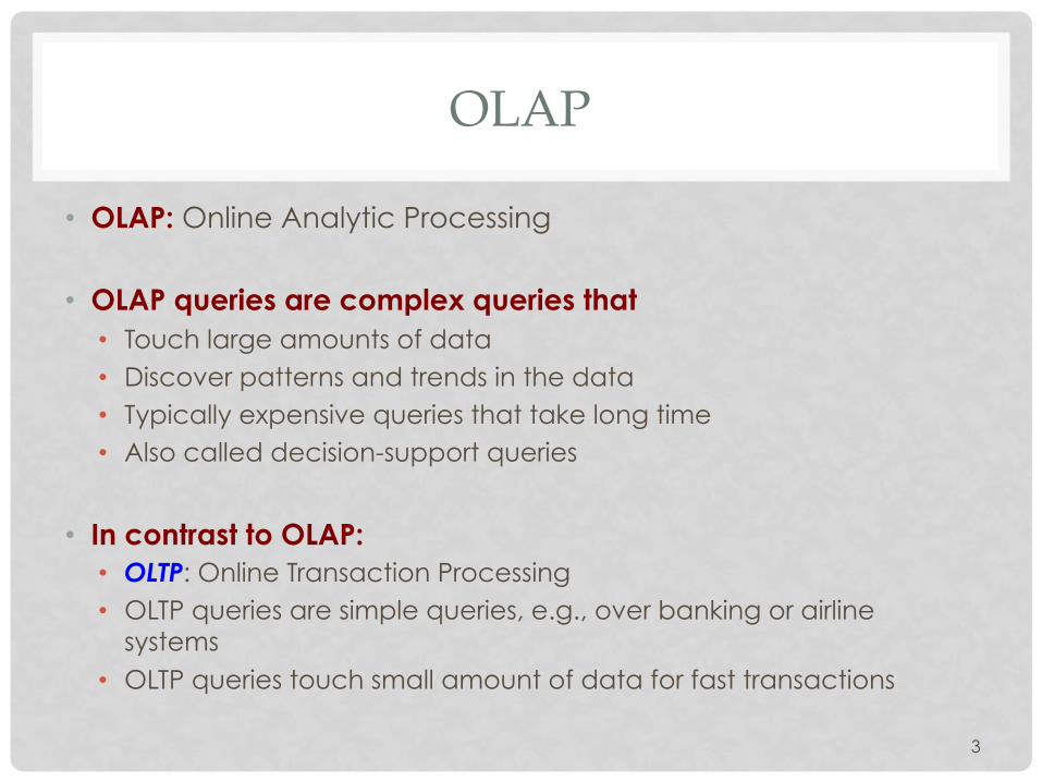
OLAP

•  OLAP: Online Analytic Processing

•  OLAP queries are complex queries that •  Touch large amounts of data •  Discover patterns and trends in the data •  Typically expensive queries that take long time •  Also called decision-support queries

•  In contrast to OLAP: •  OLTP: Online Transaction Processing •  OLTP queries are simple queries, e.g., over banking or airline

systems •  OLTP queries touch small amount of data for fast transactions

3

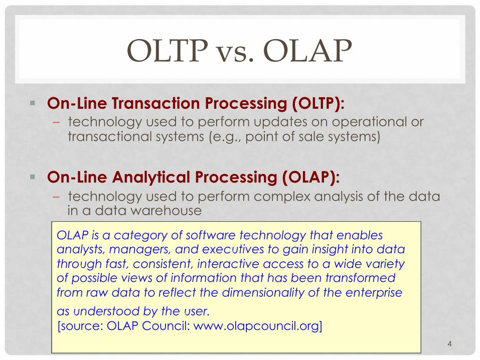
OLTP vs. OLAP

§  On-Line Transaction Processing (OLTP): –  technology used to perform updates on operational or

transactional systems (e.g., point of sale systems)

§  On-Line Analytical Processing (OLAP): –  technology used to perform complex analysis of the data

in a data warehouse

4

OLAP is a category of software technology that enables analysts, managers, and executives to gain insight into data through fast, consistent, interactive access to a wide variety of possible views of information that has been transformed from raw data to reflect the dimensionality of the enterprise

as understood by the user. [source: OLAP Council: www.olapcouncil.org]

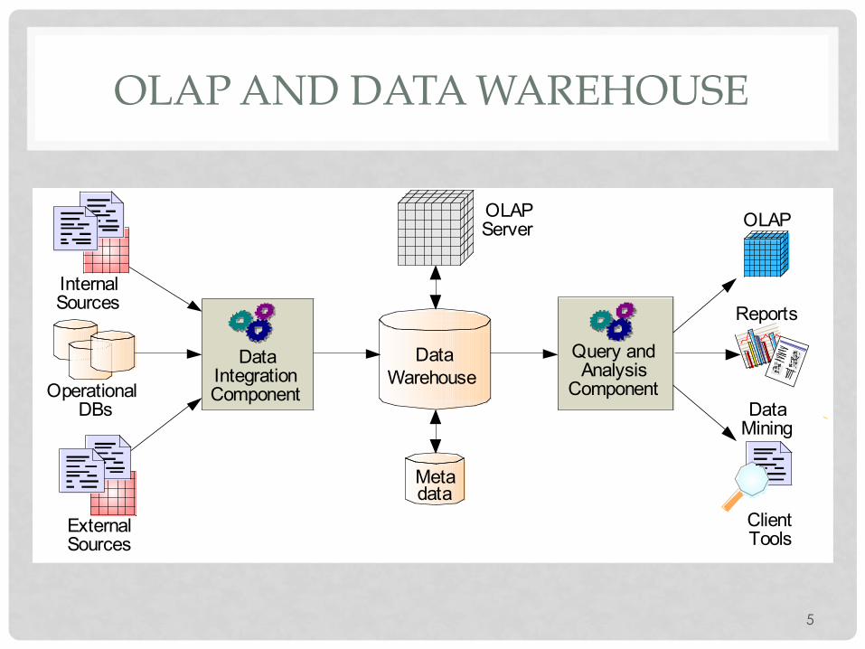
OLAP AND DATA WAREHOUSE

5

Query and Analysis

Component

Data Integration Component

Data Warehouse

Operational DBs

External Sources

Internal Sources

OLAP Server

Metadata

OLAP

Reports

Client Tools

Data Mining

OLAP AND DATA WAREHOUSE

•  Typically, OLAP queries are executed over a separate copy of the working data •  Over data warehouse

•  Data warehouse is periodically updated, e.g., overnight •  OLAP queries tolerate such out-of-date gaps

•  Why run OLAP queries over data warehouse?? •  Warehouse collects and combines data from multiple sources •  Warehouse may organize the data in certain formats to support OLAP

queries •  OLAP queries are complex and touch large amounts of data

•  They may lock the database for long periods of time •  Negatively affects all other OLTP transactions

6

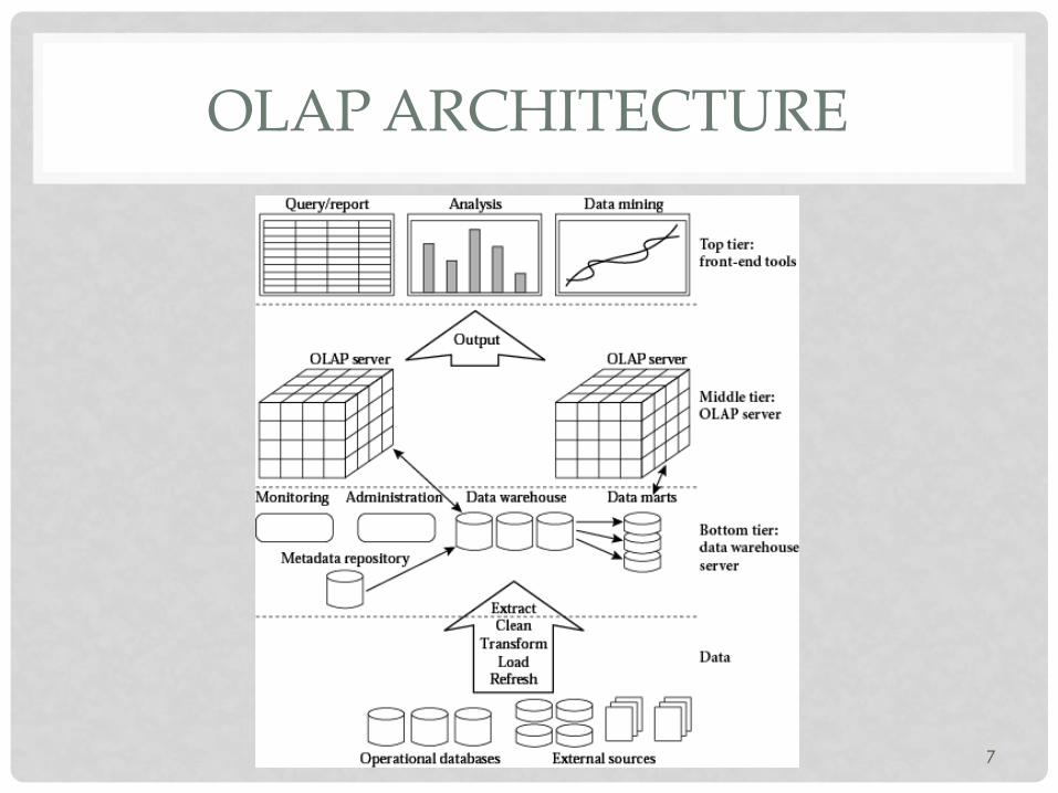
OLAP ARCHITECTURE

7

EXAMPLE OLAP APPLICATIONS

•  Market Analysis •  Find which items are frequently sold over the summer but

not over winter?

•  Credit Card Companies •  Given a new applicant, does (s)he a credit-worthy? •  Need to check other similar applicants (age, gender,

income, etc…) and observe how they perform, then do prediction for new applicant

8

OLAP queries are also called “decision-support” queries

MULTI-DIMENSIONAL VIEW

•  Data is typically viewed as points in multi-dimensional space

9

10

47

30

12 Milk 1%fat

3/1 3/2 3/3 3/4

Milk 2%fat

Orange juice

bread

Time

Items NY

MA CA

Location

Raw data cubes (raw level without

aggregation)

Typical OLAP applications have many dimensions

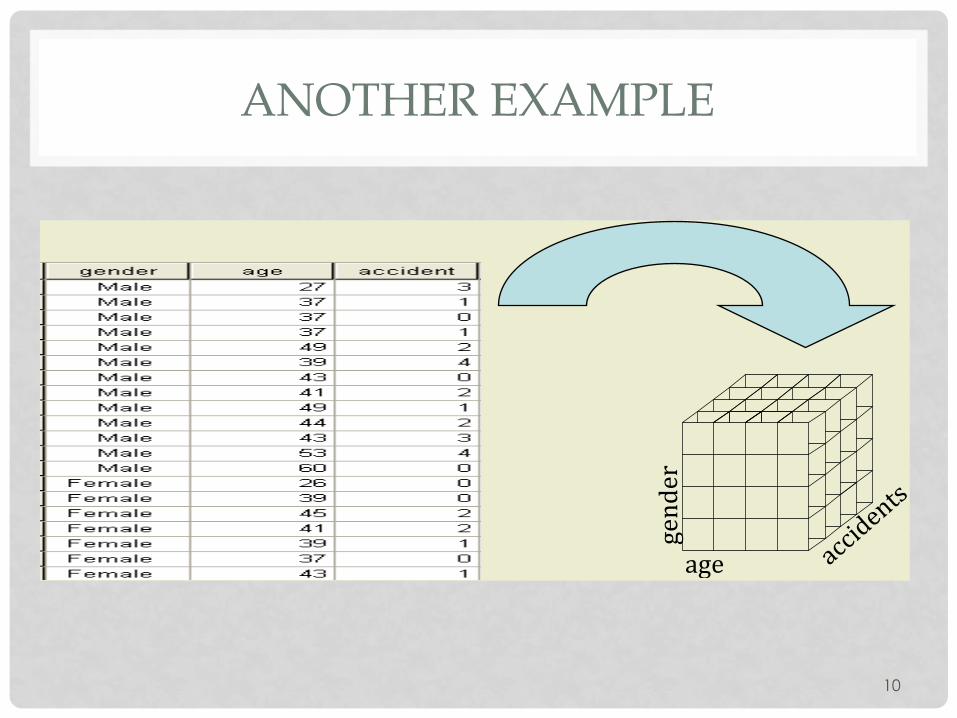
ANOTHER EXAMPLE

10

!"# !$$%&#'()

"#'&#*

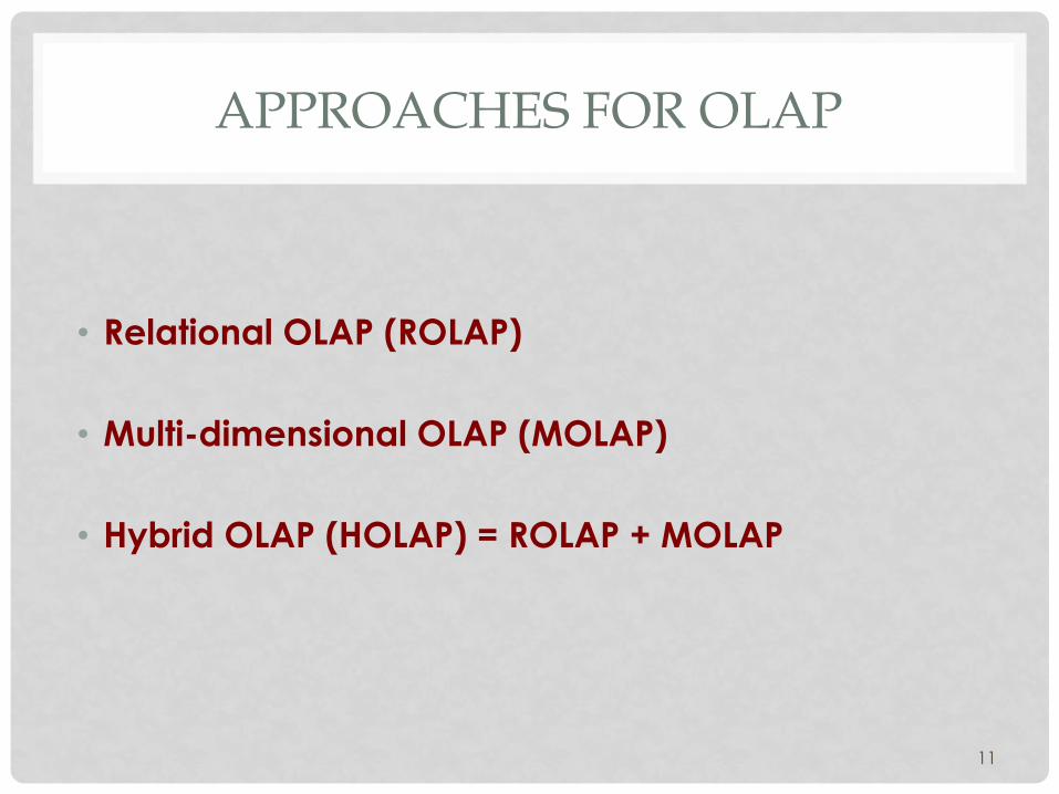
APPROACHES FOR OLAP

•  Relational OLAP (ROLAP)

•  Multi-dimensional OLAP (MOLAP)

•  Hybrid OLAP (HOLAP) = ROLAP + MOLAP

11

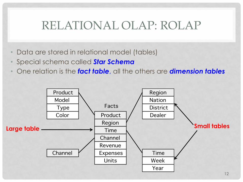
RELATIONAL OLAP: ROLAP

•  Data are stored in relational model (tables) •  Special schema called Star Schema •  One relation is the fact table, all the others are dimension tables

12

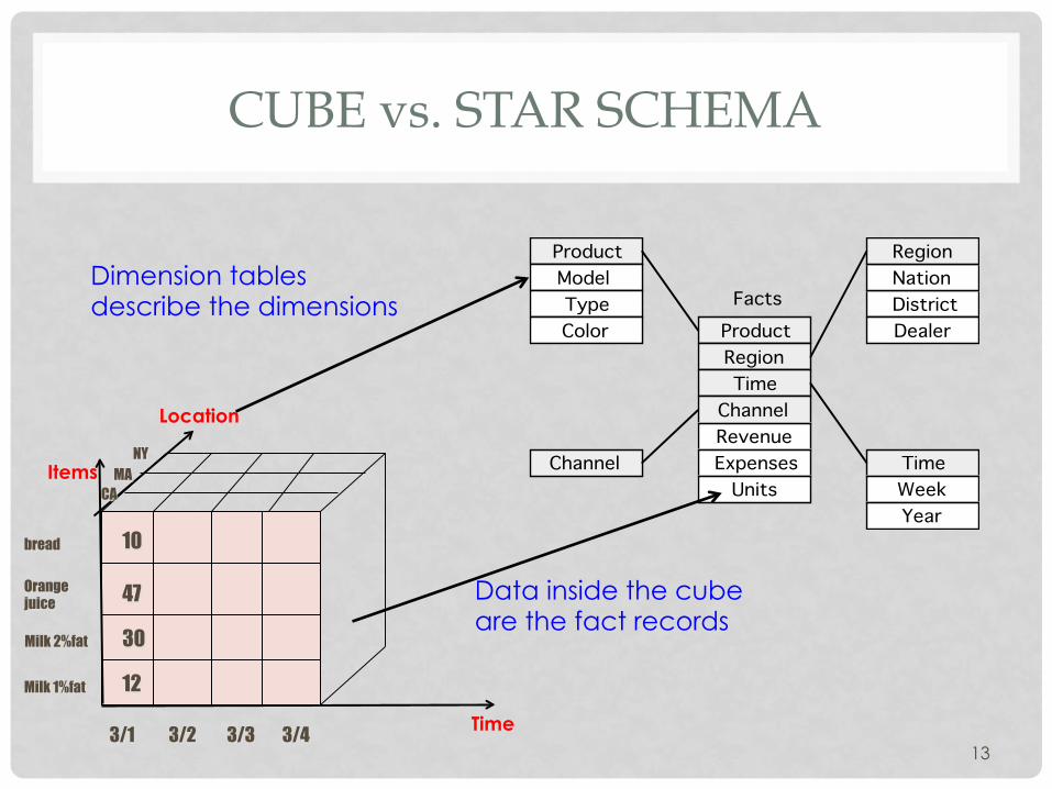
Facts

Week

Product

Product

Year

RegionTime

ChannelRevenueExpensesUnits

ModelTypeColor

Channel

RegionNationDistrictDealer

Time

Large table Small tables

CUBE vs. STAR SCHEMA

13

Facts

Week

Product

Product

Year

RegionTime

ChannelRevenueExpensesUnits

ModelTypeColor

Channel

RegionNationDistrictDealer

Time

Data inside the cube are the fact records

Dimension tables describe the dimensions

10

47

30

12 Milk 1%fat

3/1 3/2 3/3 3/4

Milk 2%fat

Orange juice

bread

Time

Items NY

MA CA

Location

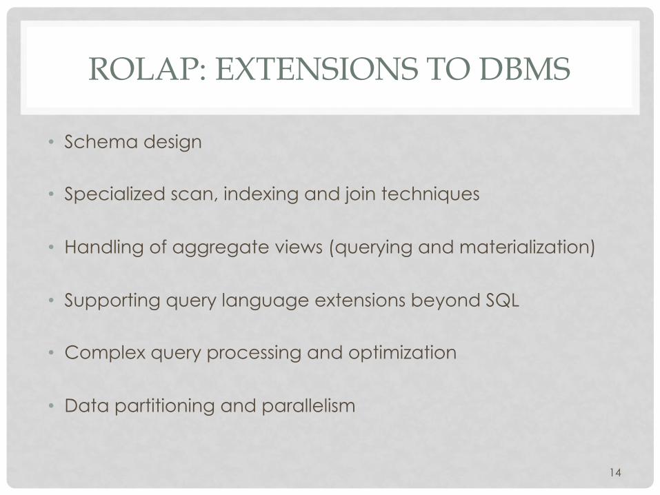
ROLAP: EXTENSIONS TO DBMS

•  Schema design

•  Specialized scan, indexing and join techniques

•  Handling of aggregate views (querying and materialization)

•  Supporting query language extensions beyond SQL

•  Complex query processing and optimization

•  Data partitioning and parallelism

14

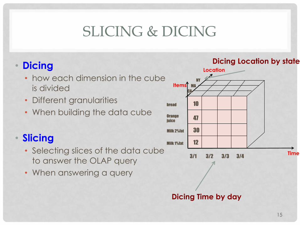
SLICING & DICING

•  Dicing •  how each dimension in the cube

is divided •  Different granularities •  When building the data cube

•  Slicing •  Selecting slices of the data cube

to answer the OLAP query •  When answering a query

15

Dicing Time by day

10

47

30

12 Milk 1%fat

3/1 3/2 3/3 3/4

Milk 2%fat

Orange juice

bread

Time

Items NY

MA CA

Location

Dicing Location by state

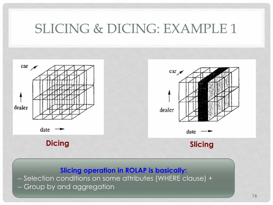
SLICING & DICING: EXAMPLE 1

16

Dicing Slicing

Slicing operation in ROLAP is basically: -- Selection conditions on some attributes (WHERE clause) + -- Group by and aggregation

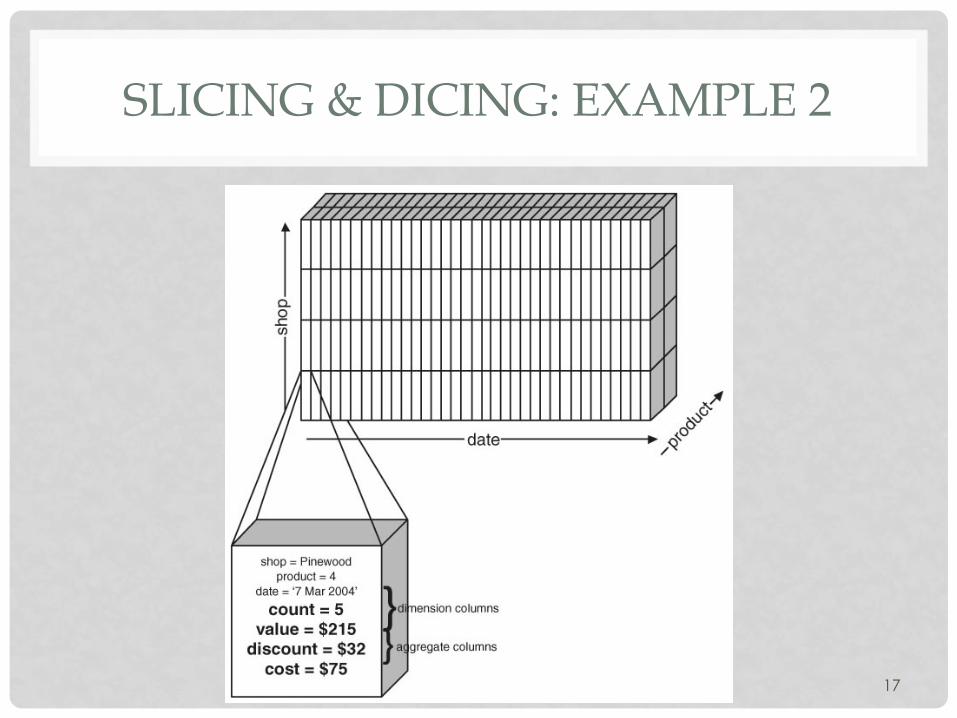
SLICING & DICING: EXAMPLE 2

17

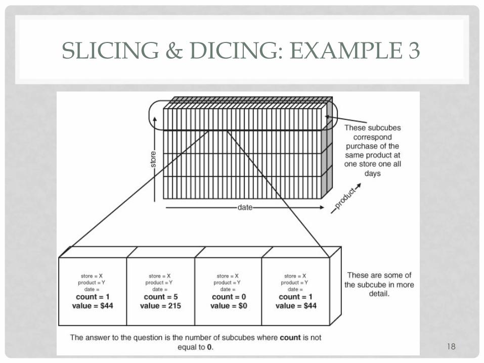
SLICING & DICING: EXAMPLE 3

18

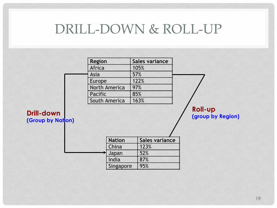
DRILL-DOWN & ROLL-UP

19

Region Sales variance

Africa 105%

Asia 57%

Europe 122%

North America 97%

Pacific 85%

South America 163%

Nation Sales variance

China 123%

Japan 52%

India 87%

Singapore 95%

Drill-down (Group by Nation)

Roll-up (group by Region)

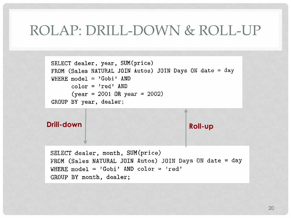
ROLAP: DRILL-DOWN & ROLL-UP

20

Drill-down Roll-up

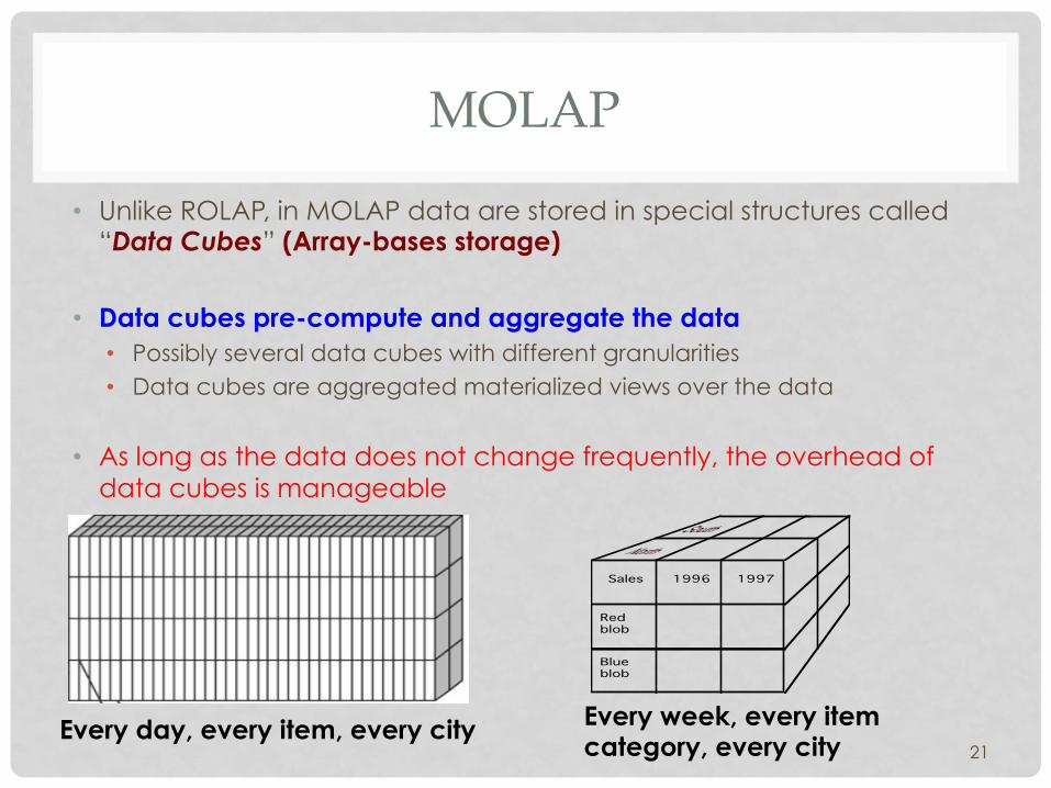
MOLAP

•  Unlike ROLAP, in MOLAP data are stored in special structures called “Data Cubes” (Array-bases storage)

•  Data cubes pre-compute and aggregate the data •  Possibly several data cubes with different granularities •  Data cubes are aggregated materialized views over the data

•  As long as the data does not change frequently, the overhead of data cubes is manageable

21

Sales 1996

Redblob

Blueblob

1997

Every day, every item, every city Every week, every item category, every city

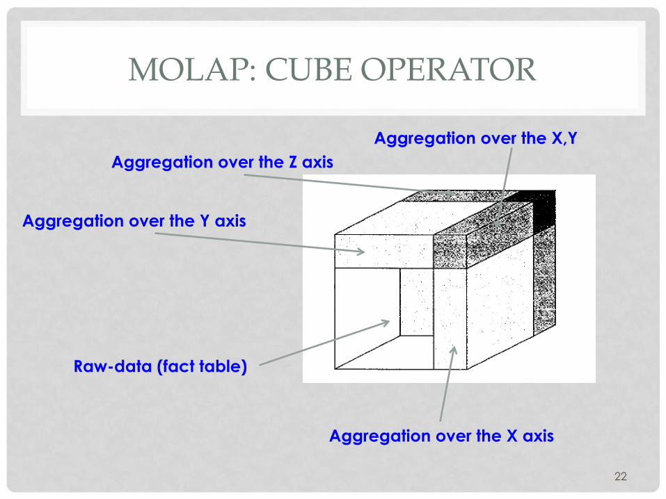
MOLAP: CUBE OPERATOR

22

Raw-data (fact table)

Aggregation over the X axis

Aggregation over the Y axis

Aggregation over the Z axis Aggregation over the X,Y

MOLAP & ROLAP

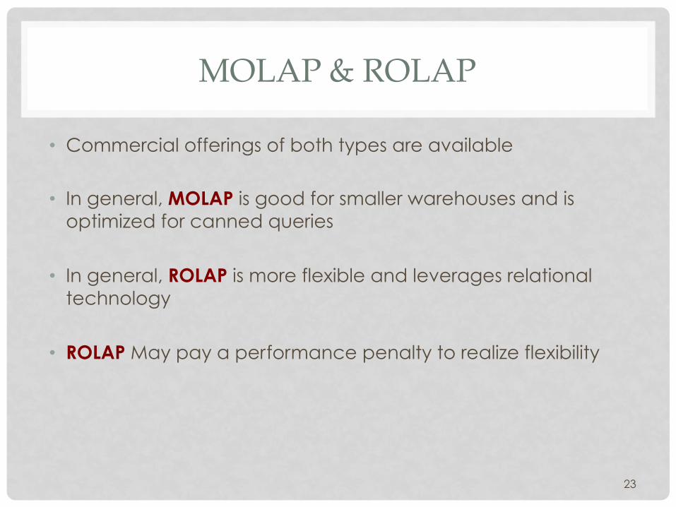
•  Commercial offerings of both types are available

•  In general, MOLAP is good for smaller warehouses and is optimized for canned queries

•  In general, ROLAP is more flexible and leverages relational technology

•  ROLAP May pay a performance penalty to realize flexibility

23

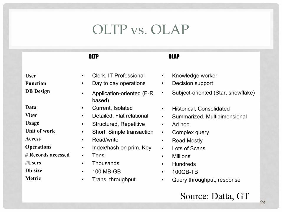
OLTP vs. OLAP

24

•  Clerk, IT Professional •  Day to day operations

•  Application-oriented (E-R based)

•  Current, Isolated •  Detailed, Flat relational •  Structured, Repetitive •  Short, Simple transaction •  Read/write •  Index/hash on prim. Key •  Tens •  Thousands •  100 MB-GB •  Trans. throughput

•  Knowledge worker •  Decision support

•  Subject-oriented (Star, snowflake)

•  Historical, Consolidated •  Summarized, Multidimensional •  Ad hoc •  Complex query •  Read Mostly •  Lots of Scans •  Millions •  Hundreds •  100GB-TB •  Query throughput, response

User Function DB Design Data View Usage Unit of work Access Operations # Records accessed #Users Db size Metric

OLTP OLAP

Source: Datta, GT

OLAP: SUMMARY

•  OLAP stands for Online Analytic Processing and used in decision support systems •  Usually runs on data warehouse

•  In contrast to OLTP, OLAP queries are complex, touch large amounts of data, try to discover patterns or trends in the data

•  OLAP Models •  Relational (ROLAP): uses relational star schema •  Multidimensional (MOLAP): uses data cubes

25

Overview on Data Mining Techniques

26

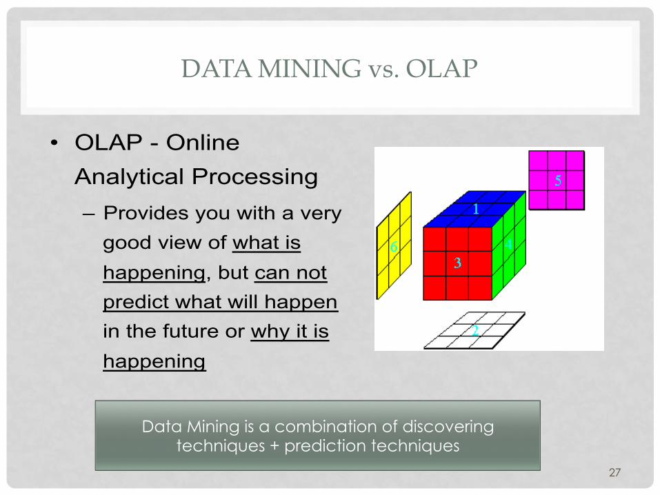
DATA MINING vs. OLAP

27

•  OLAP - Online Analytical Processing –  Provides you with a very

good view of what is happening, but can not predict what will happen in the future or why it is happening

Data Mining is a combination of discovering techniques + prediction techniques

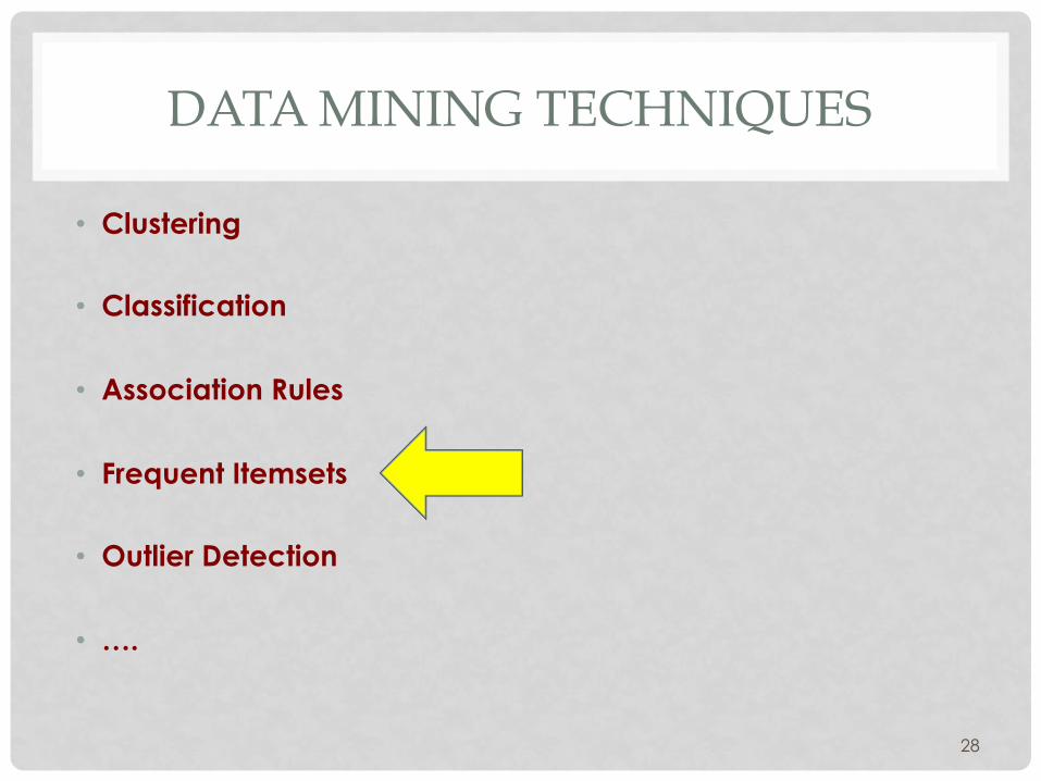
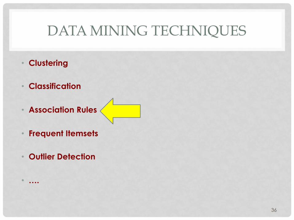
DATA MINING TECHNIQUES

•  Clustering

•  Classification

•  Association Rules

•  Frequent Itemsets

•  Outlier Detection

•  ….

28

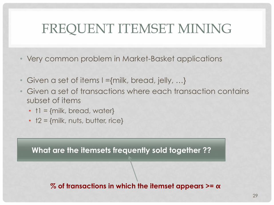
FREQUENT ITEMSET MINING

•  Very common problem in Market-Basket applications

•  Given a set of items I ={milk, bread, jelly, …} •  Given a set of transactions where each transaction contains

subset of items •  t1 = {milk, bread, water} •  t2 = {milk, nuts, butter, rice}

29

What are the itemsets frequently sold together ??

% of transactions in which the itemset appears >= α

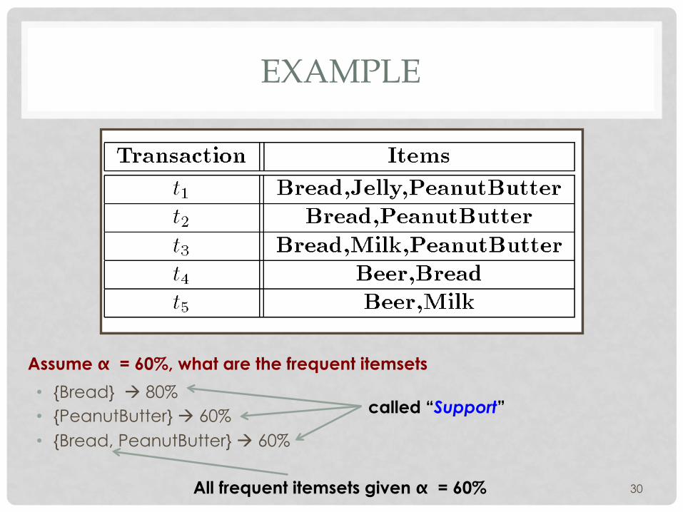
EXAMPLE

30

Assume α = 60%, what are the frequent itemsets

•  {Bread} à 80% •  {PeanutButter} à 60% •  {Bread, PeanutButter} à 60%

called “Support”

All frequent itemsets given α = 60%

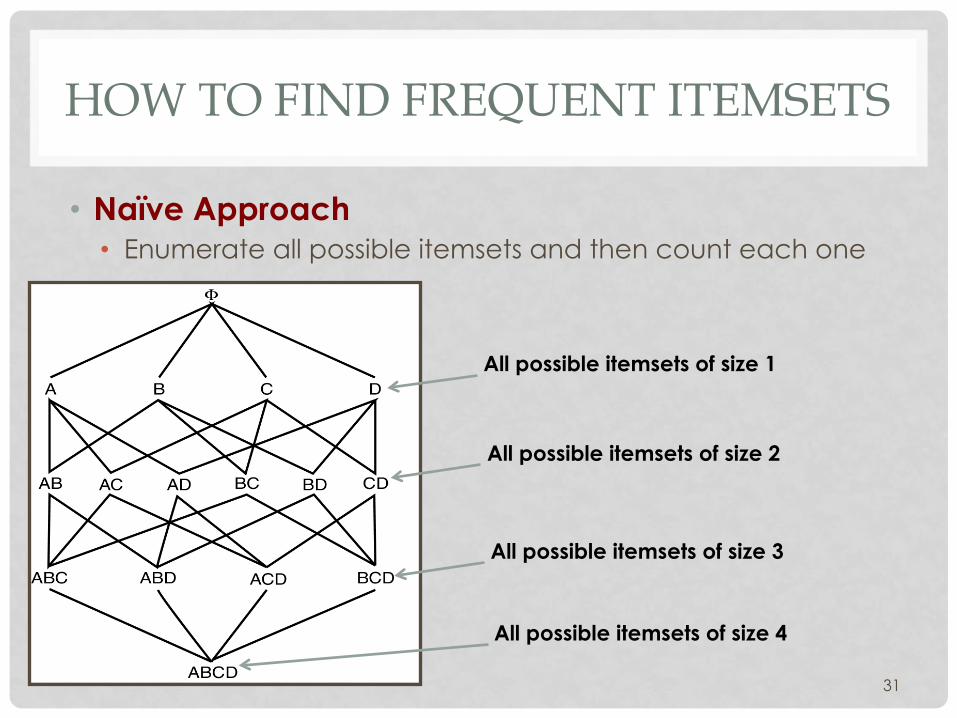
HOW TO FIND FREQUENT ITEMSETS

•  Naïve Approach •  Enumerate all possible itemsets and then count each one

31

All possible itemsets of size 1

All possible itemsets of size 2

All possible itemsets of size 3

All possible itemsets of size 4

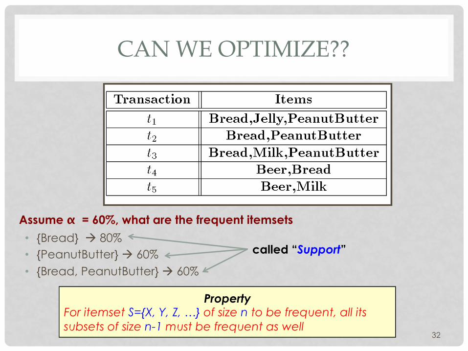
CAN WE OPTIMIZE??

32

Assume α = 60%, what are the frequent itemsets

•  {Bread} à 80% •  {PeanutButter} à 60% •  {Bread, PeanutButter} à 60%

called “Support”

Property For itemset S={X, Y, Z, …} of size n to be frequent, all its subsets of size n-1 must be frequent as well

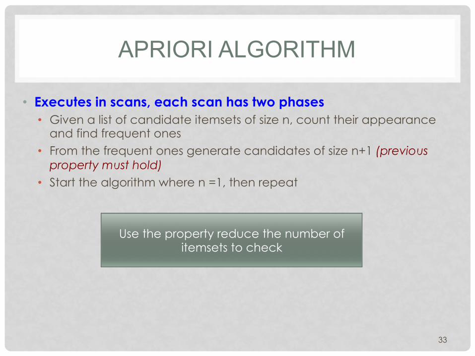
APRIORI ALGORITHM

•  Executes in scans, each scan has two phases •  Given a list of candidate itemsets of size n, count their appearance

and find frequent ones •  From the frequent ones generate candidates of size n+1 (previous

property must hold) •  Start the algorithm where n =1, then repeat

33

Use the property reduce the number of itemsets to check

APRIORI EXAMPLE

34

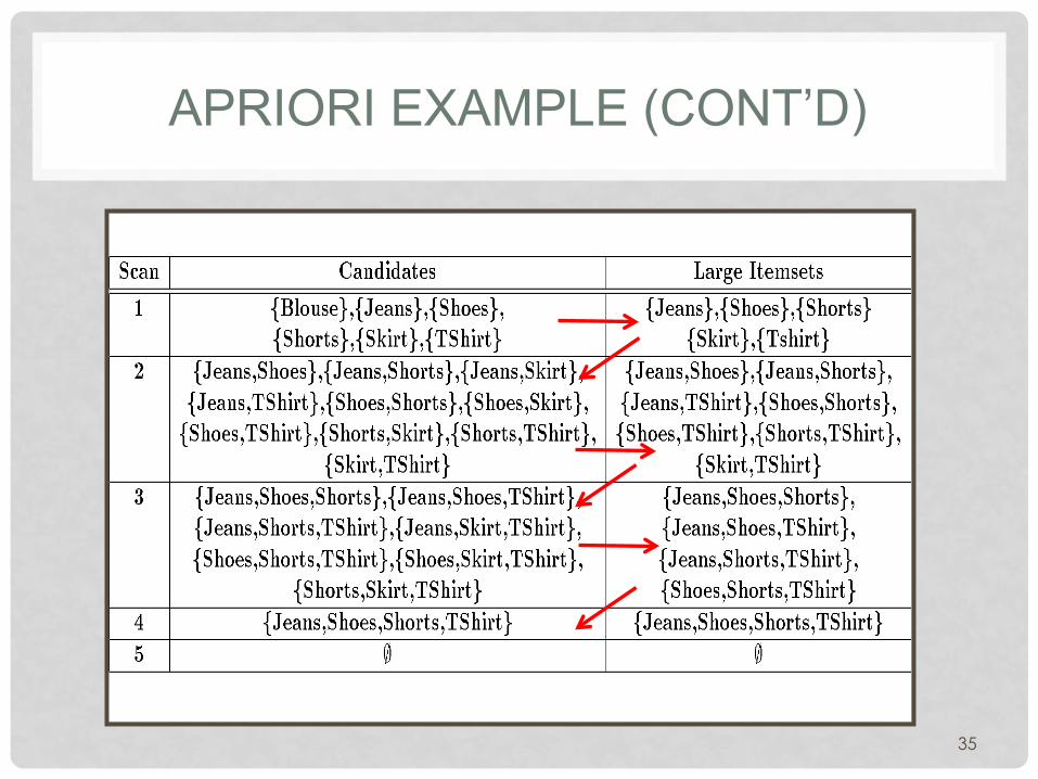
APRIORI EXAMPLE (CONT’D)

35

DATA MINING TECHNIQUES

•  Clustering

•  Classification

•  Association Rules

•  Frequent Itemsets

•  Outlier Detection

•  ….

36

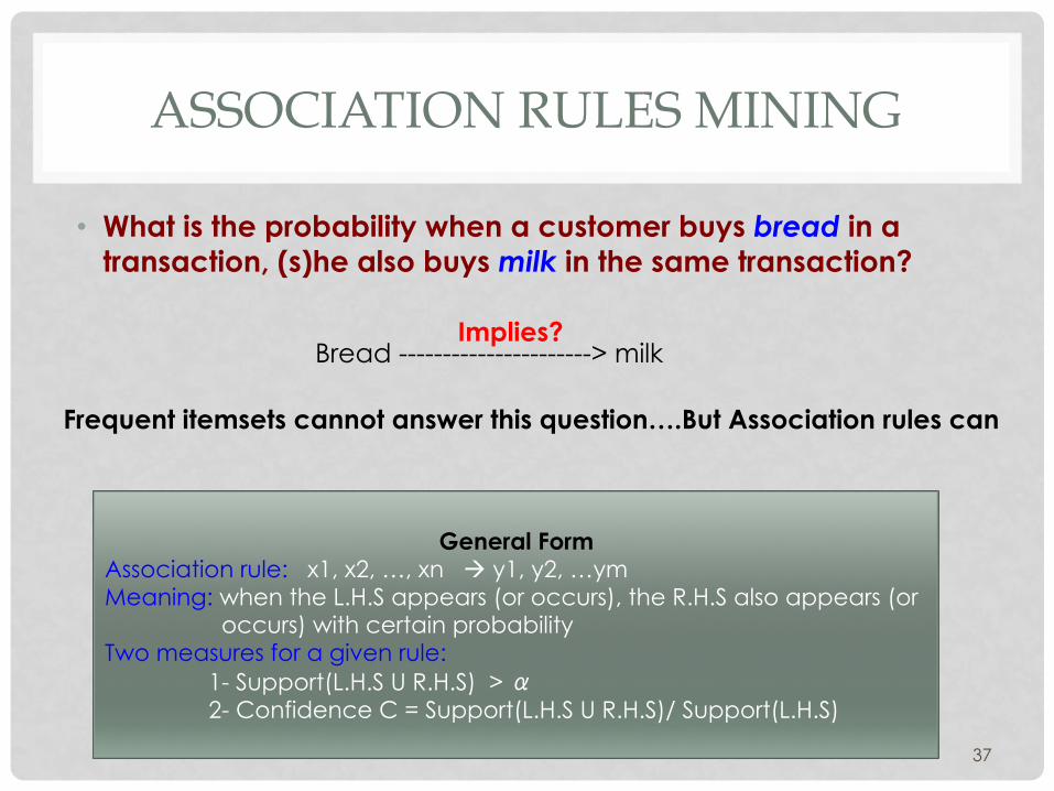
ASSOCIATION RULES MINING

•  What is the probability when a customer buys bread in a transaction, (s)he also buys milk in the same transaction?

37

Bread ----------------------> milk Implies?

Frequent itemsets cannot answer this question….But Association rules can

General Form Association rule: x1, x2, …, xn à y1, y2, …ym Meaning: when the L.H.S appears (or occurs), the R.H.S also appears (or occurs) with certain probability Two measures for a given rule: 1- Support(L.H.S U R.H.S) > α 2- Confidence C = Support(L.H.S U R.H.S)/ Support(L.H.S)

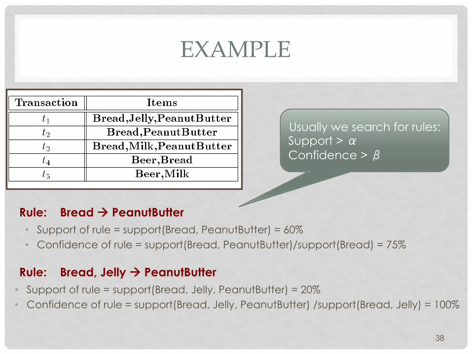
EXAMPLE

38

Rule: Bread à PeanutButter •  Support of rule = support(Bread, PeanutButter) = 60% •  Confidence of rule = support(Bread, PeanutButter)/support(Bread) = 75%

Rule: Bread, Jelly à PeanutButter •  Support of rule = support(Bread, Jelly, PeanutButter) = 20% •  Confidence of rule = support(Bread, Jelly, PeanutButter) /support(Bread, Jelly) = 100%

Usually we search for rules: Support > α Confidence > β