Okajima, Yuko
18
OSIPP Discussion Paper : DP-2016-E-003 Do “boss effects” exist in Japanese companies? Evidence from employee–supervisor matched panel data March 7, 2016 Okajima, Yuko† Specially Appointed Assistant Professor, Institute for Academic Initiatives, Osaka University Matsushige, Hisakazu Professor, Osaka School of International Public Policy (OSIPP) Ye, Yuwei Accenture Japan Ltd 【 Keywords 】 Supervisors, Managers, Performance management, Management development, Human resource development, Personnel management 【JEL Code】M12, M54 【Abstract】This paper investigates whether bosses can significantly enhance their subordinates’ performance using an eight-wave panel dataset from a medium-sized Japanese firm comprising approximately 500 employees. The dataset is of all regular employees working in one manufacturing company including in both blue-collar and white-collar occupations of various division: Product, Sales, R&D, Planning, and Admin. About 40 supervisors were matched to their subordinates, and the evaluation outcomes were used to evaluate the workers’ performance. The results showed that ‘boss effects’ were heterogeneous, displayed a one-year lag, and lasted for 2 years. It was also found that these effects remained significant, even when employees were assigned new/different supervisors. * We would like to express our gratitude to company Z for permission to use their data, and to the members of their Management Division for cooperation with interviews and discussion on the details of their personnel system. †Corresponding author. Strategic Planning Office, Institute for Academic Initiatives, Osaka University, 2-2 Yamadaoka, Suita, Osaka 565-0871, Japan. Email: [email protected]
Transcript of Okajima, Yuko
OSIPP Discussion Paper DP-2016-E-003
Do ldquoboss effectsrdquo exist in Japanese companies Evidence from employeendashsupervisor matched panel data
March 7 2016
Okajima Yukodagger
Specially Appointed Assistant Professor Institute for Academic Initiatives Osaka University
Matsushige Hisakazu
Professor Osaka School of International Public Policy (OSIPP)
Ye Yuwei Accenture Japan Ltd
【 Keywords 】 Supervisors Managers Performance management Management development Human resource development Personnel management 【JEL Code】M12 M54 【Abstract】This paper investigates whether bosses can significantly enhance their subordinatesrsquo performance using an eight-wave panel dataset from a medium-sized Japanese firm comprising approximately 500 employees The dataset is of all regular employees working in one manufacturing company including in both blue-collar and white-collar occupations of various division Product Sales RampD Planning and Admin About 40 supervisors were matched to their subordinates and the evaluation outcomes were used to evaluate the workersrsquo performance The results showed that lsquoboss effectsrsquo were heterogeneous displayed a one-year lag and lasted for 2 years It was also found that these effects remained significant even when employees were assigned newdifferent supervisors
We would like to express our gratitude to company Z for permission to use their data and to the members of their Management Division for cooperation with interviews and discussion on the details of their personnel system
daggerCorresponding author Strategic Planning Office Institute for Academic Initiatives Osaka University 2-2 Yamadaoka Suita Osaka 565-0871 Japan Email okajimaiaiosaka-uacjp
1
1 Introduction
Recently there have been many studies focusing on the reformation of personnel systems In Japan the transformation to performance-based systems has been an important issue However to increase the efficiency of personnel management it is inappropriate to focus only on the reform of the personnel system It is also necessary to focus on ldquoboss effectsrdquo because supervisors including managers play an important role in personnel management
Do bosses have a positive impact on their subordinatesrsquo performance in Japanese companies Bosses who perform well in their own jobs will not necessarily improve their subordinatesrsquo performance It is considered inefficient if bosses have no impact on their subordinatesrsquo performance in which case the allocation of managers is irrelevant It is worthwhile to focus on boss effects if managers have the potential to significantly improve their subordinatesrsquo performance However little consideration has been given to research on boss effects to date
There is a considerable amount of literature discussing the impacts of managers or CEOs on corporate behaviour Bertrand and Schoar (2003) examine manager effects on corporate behaviour in terms of different decision-making behaviours Kaplan Klebanov and Sorensen (2012) examine the particular characteristics of CEOs that are important for corporate governance Bennedsen (2007) assesses CEO effects on firm outputs However most of these studies do not consider the effects of bosses on their workers Lazear Shaw and Stanton (2012) use a bossndashworker matched dataset to study boss effects in technology-based jobs but they do not examine boss effects in white-collar occupations
The first objective of this study is to investigate whether boss effects exist in both white-collar and blue-collar occupations using a bossndashworker matched dataset from a Japanese manufacturing company (hereafter Company Z) In most of manufacturing companies in Japan permanent employees in a blue-collar occupation are commonly evaluated based on their performance and are subject to the same seniority-based pay system as white-collar workers1 It is suggested that there may be significant boss effects in Company Z Furthermore it seems that the boss effects only become apparent 1 year later (ie there is a 1-year lag) and do not disappear immediately when subordinates switch bosses The second objective is to examine the heterogeneity and trends of boss effects The analysis in this paper indicates that bosses affect their subordinates heterogeneously due to their personal management styles Therefore boss effects will become increasingly significant over time
The remainder of this paper is structured as follows Several previous studies on boss effects are
1 Koike (1996) found ldquothe white collarization of blue-collar workersrdquo by focusing on intellectual mastery and kaizen
(the concept of continuous improvement in the front-lines of manufacturing processes) among blue-collar workers in
large Japanese manufacturing companies Ishida (1990) studied the distribution of pay levels in blue-collar jobs in
Japanese manufacturing companies and concluded that this was both an incentive and a source of management
control in the manufacturing process
2
introduced in Section 2 The empirical method used to investigate boss effects in this paper is explained in Section 3 The background of the dataset and descriptions of the key variables including evaluation outcomes are presented in Section 4 Section 5 presents the results and discussion Section 6 concludes
2 Literature Review
In the field of business management the role of managers or supervisors and the performance of teams have long been debated in leadership theory Starting with the Ohio study in the late 1940s contingency theory and pathndashgoal theory sought to shed light on the relationships between leadership qualities behaviour and circumstances2 However these fundamentals of leadership theory have subsequently been extended in numerous ways and discussion has focused on the changing attitudes of subordinates In the fields of psychology and organizational behaviour in business management the subject of supervisory coaching behaviour has been discussed Although little empirical research measuring leadersrsquo behaviour and employeesrsquo performance exists Ellinger Ellinger and Keller (2003) examined the links between supervisory coaching behaviour and employee job satisfaction and performance
Because ldquofirms and employees naturally have opposing interests in that employee effort typically leads to benefits to the firms and costs to the employeerdquo (Lazear and Oyer 2013 p 480) incentives monitoring and intrinsic rewards are central issues in personnel economics Since Becker proposed the idea of human capital in 1964 Lazear (1979) and Milgrom and Roberts (1992) have gone on to discuss contract theory describing the need for purposeful design of compensation and performance systems The evaluation system is one aspect of employee monitoring and is usually administered by managers or supervisors Moreover in a well-designed incentive scheme it is the role of the CEO or managers to encourage actions that lead to goal congruence and they can avoid conflicts of interest by modifying self-interested behaviour on the part of employees
Most recently economists have used empirical studies to explore the effects of incentives on employees in relatively controlled settings Literature in various fields has examined work behaviour and workersrsquo productivity Abowd Kramarz and Woodcock (2008) developed a method to analyse the relationship between the employer and the employees (job relationship) using prototypical longitudinally linked employerndashemployee data First they introduced two specifications for their linear regression model One contained the interaction between observable and unobservable characteristics of the individuals and the firms The other was simpler only examining the pure person effects and pure firm effects Their main interest was in personfirm effects and unobservable heterogeneity In the second step they focused on a mixed model specification of the pure person effects and pure firm effects models Finally they used the estimates of the fixed effects model as a base to investigate the heterogeneity biases in the case where the person effects or the firm effects
2 Fleishman and Harris (1962)
3
were omitted They pointed out that the bias from omitting personfirm effects depended on the conditional covariance of the time-varying exogenous characteristics and the dummy variables for the firmperson effects given the dummy variables for individualsfirms
Lazear Shaw and Stanton (2012) used a similar methodology to investigate boss effects They examined the supervisorsrsquo impacts on the productivity of workers using a large sample of daily data from technology-based service jobs and found that high-quality bosses could increase teamsrsquo outputs substantially They also confirmed that the supervisorsrsquo effects on workersrsquo outputs would persist given that the bosses increased the workersrsquo productivity by teaching them new skills Finally Lazear Shaw and Stanton considered the efficient allocation of bosses They found that by allocating effective bosses high-quality workersrsquo productivity could be increased more than low-quality workersrsquo productivity However they did not investigate boss effects in white-collar occupations or their trends over time
The recent studies in the field of education the effect of principals offered insight for studies of ldquoboss effectsrdquo Branch Hanushek and Rivkin (2012) provided quantitative evidence of the impact of school principals on student outcomes They examined variations in the value added by principals by poverty quartile and found that the weakest principals were disproportionately distributed to the poorest schools They investigated principal effectiveness and found that a high-quality principal could raise student outcomes above the annual average for all students in the school They argued that principals influenced the studentsrsquo outcomes by the way in which they utilized the teaching staff
As noted the relationship between principal quality and student outcomes in schools is similar to that between CEO quality and workersrsquo productivity While Branch Hanushek and Rivkin (2102) focused on the impact of principal quality they did not consider the impacts of the teachers who influenced the students directly In other words they did not examine the effects on workersrsquo outputs of their direct bosses
Rockoff (2004) investigated the extent to which teacher qualities influence studentsrsquo achievement using a studentndashteacher matched panel dataset He used test scores for vocabulary reading comprehension mathematical computation and mathematical concepts to measure student achievement Rockoff used a random effects meta-analysis approach to confirm the existence of teacher effects The results of F-tests indicated that teacher effects were significant determinants of studentsrsquo test scores Rockoff calculated both the raw standard deviation and the estimated underlying standard deviation of teacher fixed effects Although the adjusted standard deviation was lower than the raw one it suggested that teacher qualities affected studentsrsquo achievement substantially Furthermore Rockoff proposed a correlation between teaching experience and student achievement He assumed that the teachersrsquo years of experience would have no impact on studentsrsquo test scores when they exceeded a certain cutoff point Strong evidence of gains from teaching experience was found in relation to vocabulary after controlling for teachersrsquo fixed effects The marginal return of teaching experience was positive but gradually declined as the years of experience increased until reaching the cutoff point
The application of an econometric methodology to analyse the relationship between a pair of actors is not confined to the field of education It can also be applied to the field of sports to analyse
4
coachesrsquo effects on playersrsquo performance The first study to provide empirical evidence of the robustness of estimates of coaching efficiency using English Football Association data was conducted by Dawson Dobson and Gerrard (2000) who used match outcomes to measure team performance Dawson Dobson and Gerrard used transfer values as the index of playersrsquo talent They utilized the playersrsquo characteristics including coaching input to estimate values so that the indirect impacts of coaching could be captured They found that estimates of coaching efficiency were sensitive to the choice of time-invariant efficiency models versus time-varying and inefficiency effect models The results were also sensitive to the inclusion of ex post financial input namely wage expenditure Nevertheless Dawson Dobson and Gerrard did not check for impacts on individual team members
Researchers tend to investigate the factors leading to differences in boss effects after confirming their existence and there is a wide range of studies analysing management styles Bertrand and Schoar (2003) constructed a panel dataset that matched managers and firms so that they were able to track the managers when they changed firms over time This dataset was used to investigate whether and how managers influenced corporate decision-making processes They found considerable heterogeneity among managers Bertrand and Schoar examined manager fixed effects while controlling for firm fixed effects Using F-tests for manager fixed effects they found that the managers had a significant effect on a wide range of corporate decisions including investment and acquisition decisions They also utilized the size distribution to compare the magnitude of manager fixed effects and showed that some managers had a significant impact on corporate performance In addition they analysed the relationship between managerial styles and observable managerial characteristics MBA graduation and birth cohort It was suggested that managers from earlier birth cohorts were more conservative financially Nonetheless managers who had graduated from MBA programs would make more aggressive decisions on average Although Bertrand and Schoar confirmed the manager effect on corporate decision-making they did not deal with the impacts on workers of different management styles
Borghans Weel and Weinberg (2008) considered a framework of interpersonal skills including caring and directness Their analysis used a longitudinal dataset to examine the impact of individualsrsquo sociability in their youth on their job choices in later years Their results showed that those who were sociable when they were 16 years old tended to choose jobs emphasizing interpersonal interactions Borghans Weel and Weinberg investigated the relationship between interpersonal style and labour market consequences using British and German data They found that directness provided higher returns than caring in terms of wages earned in both countries They also found that workers were most productive when they were assigned to jobs that best matched their interpersonal styles Although Borghans Weel and Weinberg examined workersrsquo wage premiums as a result of their interpersonal styles they did not investigate the relationship between workersrsquo productivity and their bossesrsquo personal management styles
3 Framework of Analysis
5
Here empirical models are developed to investigate whether boss effects exist in Company Z The main models used in this paper are ordered probit models which analyse the pooled data and panel ordered probit models which control for personal effects Using time-series data panel estimation eliminates both negative correlation and spurious correlation It is possible to hypothesize individual personal effects which are normally unobservable As the goal of this study was to prove the existence of boss effects on subordinatesrsquo performance the dependent variable was the evaluation outcome which represented the level of employee performance In addition the independent variable included dummy variables for the supervisors who evaluated their subordinatesrsquo performance and we hypothesized the existence and heterogeneity of boss effects in each evaluator Because working with high-performing colleagues tends to improve the performance of lower-performing employees the peer effect was also included as an independent variable
31 Ordered Probit Model
The evaluation outcome is not a continuous variable but rather a discrete variable ranked from 1 to 5 in ascending order of employee performance Therefore first the changes in the possibility of being rated more highly are examined using pooled data via an ordered probit model The performance of each worker is assumed to be a continuous latent variable y which is unobservable and specified as follows
yilowast = Xiζ + WEiη+ BOSSiθ + εi (1)
where yilowast stands for the performance of worker i=1hellipN and Xi is a vector of exogenous personal characteristics for worker i including age gender and years of schooling To isolate boss effects from department effects WEi is controlled for in the model WEi describes the working environment of worker i including the peer effects of his or her colleagues BOSSi is a vector of indicator variables regarded as boss effects for worker i bossij which is an element of BOSSii is 1
if the assessor of worker i is j (j=1hellipZ) and 0 otherwise The error term εi has a standard normal
distribution and are assumed to have the following properties
EεiXi WEi BOSSi = 0 Covεm εmXi WEi BOSSi = 1 if m = n0 if m ne n (2)
However we can observe yi instead of yilowast where the evaluation outcome takes values of 1 2 3 4 or 5 according to the following rules in which ki is the cutoff point
yi = 1 if and only if k0 lt yilowast le k1 ⋮
yi = 5 if and only if k4 lt yilowast le k5 (3)
Because the error terms are assumed to be independent and identically normally distributed according to Equation (2) the probability of being rated at the rth rank (r=1hellip5) is defined as follows
P(yi = r) = Φkr minus Xiζ minusWEiη minus BOSSiθ minus Φkrminus1 minus Xiζ minusWEiη minus BOSSiθ (4)
6
Then we can calculate the log-likelihood function using Equation (4) where dir = 1 if yi = r Finally the estimates of the parameters β α and γ can be calculated as follows
lnL(βα γ k1 hellip k4|yi Xi WEi BOSSi)
= lnP(yi = r)N
i=1
= sum sum dir times ln [Φkr minus Xiζ minus WEiη minus BOSSiθ minus Φkrminus1 minus Xiζ minus WEiη minus BOSSiθ]5r=1
Ni=1
(5)
32 Panel Ordered Probit Model Although an ordered probit model can provide evidence of boss effects using pooled data it
cannot control for personal effects such as initial ability To control for personal effects researchers (Bertrand and Schoar (2003) Lazear Shaw and Stanton (2012)) tend to employ a fixed effects model However a fixed effects model does not fit discrete dependent variables Hence we introduce a panel ordered probit model in which personal effects can be controlled for when the dependent variable is considered to be discrete
Similar to an ordered probit model the performance of worker i in year t is considered to be a continuous latent variable yitlowast as follows
yijtlowast = Xijtζ+ WEijtη+ BOSSjtθ+ ψi + υit (6)
where i=1hellipN and t=2008hellip2013 The definitions of Xijt and WEijt are the same as those in the ordered probit model bossijt an element of BOSSjt equals 1 if the assessor of worker i in year t is j (j=1hellipZ) ψi is defined as worker irsquos random personal effect υit refers to the error term υit has a standard normal distribution and conforms to the following assumptions
EυitX WE BOSS = 0Covυmt υntX WE BOSS = 1 if m = n0 if m ne n
Covυit υisX WE BOSS = 1 if t = s0 if t ne s and Cov(υit ψi|X WE BOSS) = 0 (7)
The observable discrete dependent variable yit is the evaluation outcome which takes values of 1 to 5 and follows similar rules to Equation (3) Compared with Equation (4) the possibilities of being rated at the rth rank after controlling for personal effects is defined as follows
Pyijt = r = Φkr minus Xijtζ minusWEijtη minus BOSSjtθ minus ψi minus Φkrminus1 minus Xijtζ minus WEijtη minus BOSSjtθ minus ψi
(8)
Based on Equation (8) we can obtain the following log-likelihood function for each worker i i=1hellipN
7
nL(ζηθ k1 hellip k4) = dr(yit) times lnPyijt = r5
r=1
T
t=1
= sum sum dryijttimes lnΦkr minus Xijtζ minus WEijtη minus BOSSjtθ minus ψi minus5r=1
Tt=1
Φkrminus1 minus Xijtζ minus WEijtη minus BOSSjtθ minus ψi (9)
In Equation (9) dryijt equals 1 if the evaluation outcome of worker i in year t is r The estimates can be obtained using the above equation
33 Likelihood-Ratio Test
To investigate the existence and heterogeneity of boss effects we employ the likelihood-ratio test after estimating the models as outlined above The likelihood-ratio test utilizes the log-likelihoods of the unrestricted and restricted models to test whether the restricted model is justified Setting θ1 as a base group for the boss dummy the null hypothesis to test for heterogeneity in boss effects is defined as follows
H0 θ2 = θ3 = ⋯ = θZ
The test statistic of the likelihood-ratio test is LR = minus2(lnLrestricted minus lnLunrestricted) where lnLrestricted and lnLunrestricted are defined as
the log-likelihood values of the restricted model and the unrestricted model respectively Under the null hypothesis the test statistic LR will approximately follow the χ2 distribution with dfunrestricted minus dfrestricted degrees of freedom where dfunrestricted and dfrestricted are the degrees of freedom of the models
4 Data
41 Background of Company Z
We use the bossndashworker matched micro personnel dataset of Company Z from 2008 to 2013 so that we can analyse boss effects using information on both the bosses and their subordinates Company Z is a regional Japanese consumer products company that has operated for nearly 100 years It has continuously expanded its scale and its annual revenue rose from 36 billion yen in 2008 to 51 billion yen in 2012 Currently Company Z is one of the leading companies in its field and supplies its products to customers throughout Japan The number of regular employees in this company increased by 40 during the 5-year period 2008ndash2013 from 310 in 2008 to 440 in 2013
Company Z has a production division that contains employees about 20 to 403 of all regular
3 For the first 3 years blue-collar employees represented about 20 of all regular employees In 2011 when an
additional factory was built the number of blue-collar employees rose to nearly 40 of all regular employees
8
employees The ratio of blue-collar employees working on the production line including the bottling process accounts for approximately 30 of all regular employees over an entire period Around 25 of all regular employees belong to the sales division approximately12 belong to the RampD division including RampD and the quality assurance department and around 10 belong to the planning (new business) division Other minor divisions namely the administrative division and the food service division comprise less than 5 of all employees each
The employeesrsquo performance is used as the criterion for the evaluation of outcomes The employees are rated on a scale of 1 to 5 which in ascending order represent rankings of C (poor performance) B (not meeting requirements) AB (fulfilling requirements) A (above requirements) and S (outstanding performance) respectively The ratings distribution within each department or division is never regulated The assessors of the employeesrsquo performance are their direct supervisors because they train and supervise their subordinates In this paper the term ldquobossesrdquo mentioned refers to these direct supervisors
The mechanism for evaluating the performance of employees is as follows The evaluation system was comprised of two parts behaviour evaluation and achievement evaluation With regard to behaviour evaluation specific behaviour-evaluation items were distilled based on competency consistency and conformity with the firmrsquos philosophy management policy and behavioural guidelines Achievement evaluation was assessed based on performance in the management by objectives (MBO) system The MBO system and operating rules were reformed to foster goal sharing among top-ranking managers and employees Individual goals were linked to workplace goals which were extensions of division or company goals
This evaluation system was introduced in April 2007 as a reform of the former system At the same time they introduced a reformed MBO system The evaluation outcomes used in this study are all based on the reformed system Company Z also tried to ensure the transparency of their new personnel system Training for assessors under the new evaluation system was carried out every year after its launch This training was aimed at deepening the understanding of the evaluation items in the new employee evaluation system and consisted of lectures and practical training in the evaluation methods The company gathered voice of employees through the CEO-members group interviews
42 Summary Statistics
The dataset used in this study comprises 2263 observations of regular employees from 2008 to 2013 including 1093 observations of employees whose bosses were different from the previous year This dataset provides the foundation to analyse boss effects
First the dependent variable needs to be considered Here the evaluation outcomes are used as the dependent variable It is assumed that all workers are evaluated objectively based on the evaluation rules introduced above Lazear Shaw and Stanton (2012) used the outputs of technology-based service jobs as the dependent variable to measure productivity However this method was of limited value in blue-collar occupations Hence this study uses the evaluation outcomes as the dependent variable so that productivity in white-collar occupations can also be measured
9
In this micro personnel dataset 2016 observations have evaluation outcomes These outcomes are ranked from 1 to 5 where a rank of 5 refers to the best outcomes As can be seen in Table 1 the mean evaluation outcome of employees is 376 This indicates that on average both blue-collar and white-collar employees are rated at the 3rd rank (AB) This is further illustrated by the left-skewed distribution of evaluation outcomes shown in Figure 1 However the distribution of evaluation outcomes is varied in its shape especially in year 2011 every distributions is still similar left-skewed as shown in Figure 2
(place Figure 1 here)
(place Figure 2 here)
Second the list of personal characteristics can be seen in Table 1 The average age of the subjects
in this study is about 33 years and 26 are female There is obvious polarization in employeesrsquo educational backgrounds4 To enable quantitative control educational background is translated into years of schooling which is a continuous variable As can be seen in Table 1 most of the employees have been educated for 14 years which suggests attainment of either a high school or technical college diploma This may be the result of the existence of large numbers of factory workers and senior employees who joined the company as blue-collar employees and rose to become managers5 Furthermore peer effects are also controlled for as a characteristic of the working environment Peer effects are calculated as the average evaluation outcomes of colleagues of the individuals concerned and have a mean of 37 Because this study investigates lagged boss effects the lagged characteristics are also controlled for in the analysis
During this analysis considerable attention must be paid to the endogeneity problem For example better bosses may be assigned to supervise more workers and the time for teaching per subordinates gets lower which would create a downward bias in the observed effect on subordinatesrsquo performance Alternatively high-performing subordinates may be assigned to effective bosses which would create an upward bias in the observed effect of subordinatesrsquo performance
(place Table 1 here)
5 Results
51 Heterogeneity in Boss Effects
The results shown in Table 2 indicate that bosses have an impact on their subordinatesrsquo evaluations Panel A shows the results for the ordered probit model using pooled data Panel B shows
4 Educational attainment is classified into eight categories secondary school technical and vocational training
school high school special vocational school junior college technical college university and postgraduate
education (eg masterrsquos degree andor doctorate)
5 Since Company Z is a typical Japanese manufacturing company they provides a career path to the management
level for high-performing blue-collar employees
10
the results of the panel ordered probit model which takes personal effects into account The dependent variables of estimation in Table 2 are the same (ie the employeesrsquo evaluation outcomes) taking values of 1ndash5 However the independent variables that are controlled vary Estimations A0 and B0 control the boss dummies and peer effects of department in the year of the workersrsquo performances are evaluated The boss dummies and peer effects that are controlled for in Estimations A1 and B1 and Estimations A2 and B2 are 1- and 2-year lagged respectively For example in Estimations A0 A1 and A2 worker irsquos boss dummies in 2010 2009 and 2008 respectively are controlled for if the dependent variable takes the value of his or her evaluation outcome in 2010
The likelihood-ratio test is used to confirm the existence of boss effects and variations in boss effects among bosses As can be seen in Table 2 the null hypothesis that boss effects do not differ from boss to boss is rejected at the 5 significance level in Estimations A1 A2 B1 and B2 These results illustrate that 1- and 2-year lagged boss effects both vary significantly from boss to boss when previous working environment characteristics are controlled for regardless of whether individual effects are controlled for or not It is therefore suggested that time-lagged boss effects exist in Company Z
The results indicate that bosses who have supervised them previously have an impact on workersrsquo current performance In other words boss effects become apparent a year later and last for more than 2 years which may be considered to be the consequence of teaching This result is in line with the findings of Lazear Shaw and Stanton (2012) and Ellinger and Keller (2003) who suggested that one of the basic activities of bosses is teaching the effects of which can persist over time Boss effects can last for a long period of time in employeesrsquo careers due to the effects of skill transfer and good working habits learned from their bosses
The variation in lagged boss effects among bosses is still observed when the workersrsquo personal effects are controlled for in Estimations B0 B1 and B2 as seen in Table 2 This indicates that the variation in boss effects is not caused by the different characteristics of the workers themselves but by the consequences of the personal management styles of previous bosses The rejection of the null hypothesis at the 1 significance level in Estimations B1 and B2 indicates that boss effects from previous bosses are heterogeneous In other words the heterogeneity of boss effects becomes apparent a year later and lasts for at least 2 years owing to the different management styles of bosses The finding that current bosses do not have an impact on workersrsquo performance suggests that the impact of bosses through for example teaching may require considerable time
(place Table 2 here)
52 How do Boss Effects Change
The analysis outlined above confirms that boss effects may vary from boss to boss even during the same period Therefore we need to investigate the relationship between current boss effects and the lagged boss effects How do boss effects change over time In order to investigate changes in boss effects we compare the p-values of the likelihood-ratio tests of all estimations because the
11
p-values of likelihood-ratio tests indicate the strength of the restrictions As can be seen in Table 26 the p-value for the likelihood-ratio test in Estimation B0 is the largest among Estimations B0ndashB2 This suggests that boss effects are becoming more significant over time ie bosses are having a greater impact on their subordinatesrsquo performance This finding seems reasonable if the workers are supervised by the same bosses across different periods because the bosses can reinforce their impact over a longer period
53 Robustness Check
This study uses different samples to investigate the robustness of the results outlined above In one sample the workers switch bosses during the previous year while in the other sample the workers switch bosses from 2 years earlier Table 3 shows the results It is found that the null hypothesis is rejected at the 1 significance level in the sample in which the workers switch bosses during the previous year (Bd1) and at the 10 significance level in the sample in which the workers switch bosses from 2 years earlier (Bd2) These results indicate that boss effects vary from boss to boss regardless of whether the workers switch bosses that is the results confirming the existence and heterogeneity of boss effects are robust
As can be seen in Table 3 the lagged boss effects can last even when the worker switches bosses That is boss effects remain robust after eliminating the fixed optimistic evaluations under same pair of a supervisor and a subordinate
It can be seen from Table 2 that the p-value of the likelihood-ratio test in Estimation B0 is the largest among the three estimations B0ndashB2 while the p-values of the likelihood-ratio test in Estimations B1 and B2 are nearly the same This result is in line with that for Estimations A0ndashA2 in Table 2 However a slightly different result is shown in Table 3 where it can be seen that the p-value of the likelihood-ratio test in Estimation Bd1 is much smaller than that in Estimation Bd2 This indicates that the 1-year lagged boss effects are more significant than the 2-year lagged boss effects when the workers switch bosses Because the workers have different bosses over a 2- or 3-year period the bosses cannot maintain their impact Hence the boss effects are less significant over time
(place Table 3 here)
6 Conclusion
The primary objective of this study is to document the existence and heterogeneity of boss effects
in a single Japanese company We use an ordered probit model to analyse the pooled data and a panel ordered probit model to investigate the boss effects after controlling for personal effects The
6 Because workersrsquo individual effects are controlled for in the panel ordered probit model the results of the panel
ordered probit model are more convincing than those of the ordered probit model Therefore we focus on the panel
ordered probit model when comparing the p-values of the likelihood-ratio tests
12
analysis results in two findings First it is found that previous bosses have a significant impact on their subordinatesrsquo evaluation outcomes Furthermore these boss effects last for at least 2 years because a part of these effects is the consequences of teaching In other words in the first year bosses do not have a teaching or coaching effect Along with the finding of former literature that examined 6- and 12-month lagged boss effects this study demonstrated the boss effects lasting even longer term as proving the 2-year lagged boss effects Second there are significant variations in boss effects in the second year after a change of boss This suggests that boss effects vary from boss to boss because each boss has his or her own management style
These results have some implications for company management Because the boss effects exist from the second year and last for at least for 2 years it would seem better to focus on the training of bosses to improve their subordinatesrsquo performance Further to the findings of previous studies that examined six-month and 12-month lagged boss effects this study demonstrated that the boss effects last for even longer periods of time as proved by the 2-year lagged boss effects This is mainly due to the bossesrsquo teaching activities Therefore those workers whom the company expects to promote to supervisory positions should have both sophisticated professional skills and excellent teaching skills In addition each boss has a unique way of supervising and training his or her subordinates Hence it is likely that boss effects will be improved by increasing communication among bosses such that they can share their experiences and learn from one another Because coaching skills represent another important factor that has an effect on subordinatesrsquo performance boss effects will also be improved by training bosses in communication skills Finally it is better to focus not only on employeesrsquo current bosses but also on their previous ones Furthermore it is better if workers do not switch bosses frequently such that the bosses have sufficient time to reinforce their impact on their subordinates
Although this study investigates the existence heterogeneity and trends of boss effects in both white-collar and technology-based jobs there are several limitations in the analysis It is difficult to discuss and compare boss effects in technical occupations with those in white-collar occupations such as those in the sales division RampD division and planning division because the sample size of the data used in this paper is not large enough to be divided into two parts Additionally although the evaluation outcomes can capture not only the results of performance but also the workersrsquo attitudes during the process the evaluation outcomes as a surrogate variable of performance may be limited by the evaluation distribution As a result the evaluation outcomes may reflect the relative performance results rather than the absolute ones These limitations will be addressed in future studies
Reference Abowd J M Kramarz F and Woodcock S (2008) lsquoEconometric analysis of linked
employer-employee datarsquo in L Maacutetyaacutes and P Sevestre (eds) The Econometrics of Panel Data Berlin Springer Berlin Heidelberg
13
Bennedsen M Perez-Gonzalez F and Wolfenzon D (2006) lsquoDo CEOs matterrsquo NYU Working Paper No FIN-06-032
Bertrand M and Schoar A (2003) lsquoManaging with style the effect of managers on firm policiesrsquo Quarterly Journal of Economics CXVIII 4 1169ndash1208
Borghans L Baster W and Bruce A W (2008) lsquoInterpersonal styles and labor market outcomesrsquo The Journal of Human Resources 43 4 815ndash858
Branch G F Hanushek E A and Rivken S G (2012) lsquoEstimating the effect of leaders on public sector productivity The case of school principalsrsquo Working Paper No 17803 National Bureau of Economic Research
Dawson P Dobson S and Gerard B (2000) lsquoEstimating coaching efficiency in professional team sports Evidence from English association footballrsquo Scottish Journal of Political Economy 47 4 399ndash421
Ellinger A D Ellinger A E and Keller S B (2003) lsquoSupervisory coaching behavior employee satisfaction and warehouse employee performance A dyadic perspective in the distribution industryrsquo Human Resource Development Quarterly 14 4 435ndash458
Ishida M (1999) Chingin no Shakai-kagaku [Social Science of Compensation] ndash Japan and England - Tokyo Chuo-keizai-sha
Kaplan S N Mark M K and Morten S (2012) lsquoWhich CEO characteristics and abilities matterrsquo The Journal of Finance 67 3 971ndash1005
Koike K (1996) The Economics of Work in Japan Tokyo LTCB International Library Foundation
Lazear E P Shaw K L and Stanton C T (2012) lsquoThe value of bossesrsquo Working Paper No 18317 National Bureau of Economic Research
Rockoff J E (2004) lsquoThe impact of individual teachers on student achievement evidence from panel datarsquo The American Economic Review 94 2 247ndash252
14
Figure 1 Distribution of evaluation outcomes
Evaluation Outcomes
Figure 2 Distribution of evaluation outcomes in each year
Year
0
10
20
30
40
50
60
1 2 3 4 5C B AB A S (Poor (Under (Fulfilling (Above (Outstanding Performance ) Requirements) Requirements) Requirements) Performance)
0
10
20
30
40
50
60
70
2008 2009 2010 2011 2012 2013
C (Poor Performance)
B (Under Requirements)
AB (fulfilling Requirements)
A (above Requirements)
S (Outstanding Performance)
15
Table 1 Summary statistics
Variable Definition Obs Mean Std Dev Min Max
Dependent VariableEvaluation Evaluation outcome of the employee 2016 376 074 10 50
Personal CharacteristicsAge Age of the employee (at the time evaluated) 2102 3328 1059 182 593Age (squared) Squared value of age of the employee (at the time evaluated) 2102 121966 80352 3300 35106Gender Gender of the employee 2283 026 044 00 20Years of Schooling Schooling years of the employee 2276 1404 238 90 180
Working EnvironmentEvaluation_Peers Average evaluation outcomes of colleagues 2229 375 034 20 50Evaluation_Peers_lag1 Average evaluation outcomes of colleagues 1 year lagged 1771 374 032 20 50Evaluation_Peers_lag2 Average evaluation outcomes of colleagues 2 years lagged 1333 372 033 25 50
Subsize Scale of the departement in which the employee works 2102 2483 2276 10 760Subsize_lag1 Scale of the departement in which the employee works 1 year lagged 1918 2464 2162 10 760Subsize_lag2 Scale of the departement in which the employee works 2 years lagged 1499 2436 2099 10 760
16
Table 2 Regressions of evaluations using the ordered probit model and the panel ordered probit model
PANEL A Orderd Probit Model PANEL B Panel Orderd Probit ModelA0 A1 A2 B0 B1 B2
Variable Base-year data 1-year lagged data 2-year lagged data Base-year data 1-year lagged data 2-year lagged data
Age 0129 0084 0128 0142 0084 0136-0024 (0028) (0035) -0031 (0033) (0045)
Age (squared) -0002 -0001 -0002 -0002 -0001 -0002(0000) (0000) (0000) (00002) (0000) (0001)
Gender -0046 -0124 -0120 -0088 -0148 -0165(0081) (0092) (0110) (0106) (0105) (0139)
Years of Schooling -0042 -0017 -0024 -0043 -0015 -0019(0017) (0019) (0022) (0022) (0022) (0028)
Blue Collar Dummy dagger 0009 -0099 -0064 -0041 -0149 -0161(0099) (0108) (0120) (0119) (0120) (0148)
Peer Effect 1818 2018(0123) (0130)
Peer Effect -1 -0109 -0172(0132) (0137)
Peer Effect -2 0240 -0024(0182) (0186)
Assessor Dummies yes yesAssessor Dummies -1 yes yesAssessor Dummies -2 yes yes
Year Dummies Dagger yes yes yes yes yes yes
Likelihood-ratio test for null hypothesis Boss effects are equal to each other among bosses (θ2=θ3=hellip=θZ) (θ2=θ3=hellip=θZ)
LR chi2 statistic 4511 7829 8223 2263 7666 7269Prob gt chi2 0232 0000 0000 0983 0000 0000
Log Likelihood -1423829 -1171069 -816224 -1422509 -1171386 -817303 Pseudo R2 0133 00513 0085Observations 1523 1137 825 1523 1137 825Number of id 403 367 352Standard errors in parentheses plt001 plt005 plt01
17
Table 3 Estimation using the sample in which workers have different bosses from the previous year (Panel Bd1) and from two years ago (Panel Bd2)
PANEL Bd
Panel Orderd Probit ModelBd1 Bd2
Variable 1-year lagged data 2-year lagged data
Age 0057 0136(0037) (0050)
Age (squared) -0001 -0002(0000) (0001)
Gender -0182 -0146(0114) (0142)
Years of Schooling 0012 -0042(0024) (0031)
Blue Collar Dummy dagger -0075 -0226(0146) (0164)
Peer Effect -1 -0140(0179)
Peer Effect -2 0417(0219)
Assessor Dummies -1 yesAssessor Dummies -2 yes
Year Dummies Dagger yes yes
Likelihood-ratio test for null hypothesis Boss effects are equal to each other among bosses (θ2=θ3=hellip=θZ)
LR chi2 statistic 6981 4711Prob gt chi2 0001 0067
Log Likelihood -724395 -545589Observations 708 463Number of id 321 279Standard errors in parentheses plt001 plt005 plt01
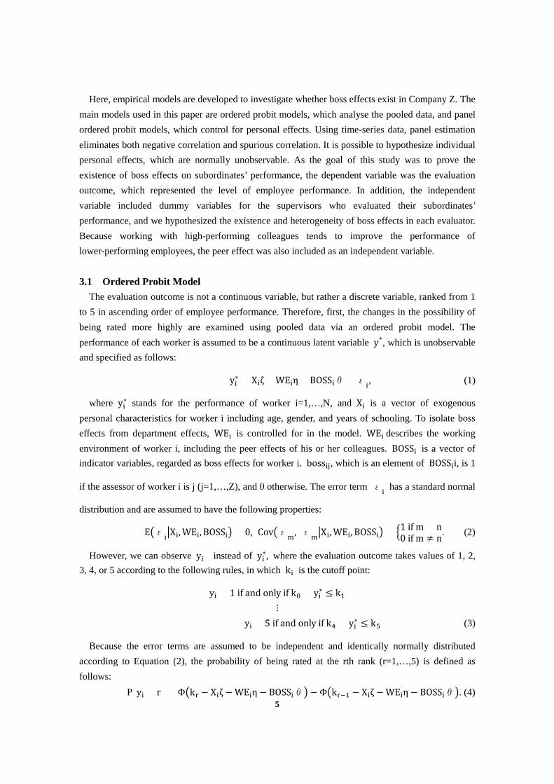
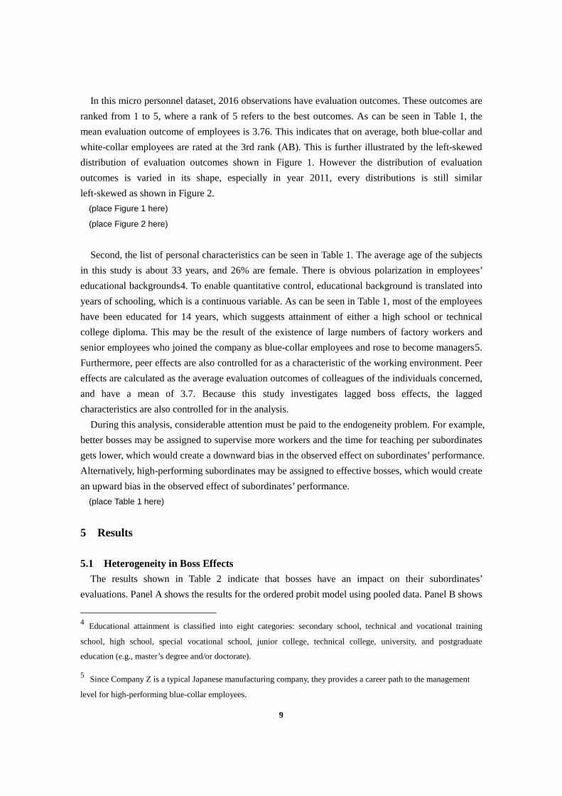

10
the results of the panel ordered probit model which takes personal effects into account The dependent variables of estimation in Table 2 are the same (ie the employeesrsquo evaluation outcomes) taking values of 1ndash5 However the independent variables that are controlled vary Estimations A0 and B0 control the boss dummies and peer effects of department in the year of the workersrsquo performances are evaluated The boss dummies and peer effects that are controlled for in Estimations A1 and B1 and Estimations A2 and B2 are 1- and 2-year lagged respectively For example in Estimations A0 A1 and A2 worker irsquos boss dummies in 2010 2009 and 2008 respectively are controlled for if the dependent variable takes the value of his or her evaluation outcome in 2010
The likelihood-ratio test is used to confirm the existence of boss effects and variations in boss effects among bosses As can be seen in Table 2 the null hypothesis that boss effects do not differ from boss to boss is rejected at the 5 significance level in Estimations A1 A2 B1 and B2 These results illustrate that 1- and 2-year lagged boss effects both vary significantly from boss to boss when previous working environment characteristics are controlled for regardless of whether individual effects are controlled for or not It is therefore suggested that time-lagged boss effects exist in Company Z
The results indicate that bosses who have supervised them previously have an impact on workersrsquo current performance In other words boss effects become apparent a year later and last for more than 2 years which may be considered to be the consequence of teaching This result is in line with the findings of Lazear Shaw and Stanton (2012) and Ellinger and Keller (2003) who suggested that one of the basic activities of bosses is teaching the effects of which can persist over time Boss effects can last for a long period of time in employeesrsquo careers due to the effects of skill transfer and good working habits learned from their bosses
The variation in lagged boss effects among bosses is still observed when the workersrsquo personal effects are controlled for in Estimations B0 B1 and B2 as seen in Table 2 This indicates that the variation in boss effects is not caused by the different characteristics of the workers themselves but by the consequences of the personal management styles of previous bosses The rejection of the null hypothesis at the 1 significance level in Estimations B1 and B2 indicates that boss effects from previous bosses are heterogeneous In other words the heterogeneity of boss effects becomes apparent a year later and lasts for at least 2 years owing to the different management styles of bosses The finding that current bosses do not have an impact on workersrsquo performance suggests that the impact of bosses through for example teaching may require considerable time
(place Table 2 here)
52 How do Boss Effects Change
The analysis outlined above confirms that boss effects may vary from boss to boss even during the same period Therefore we need to investigate the relationship between current boss effects and the lagged boss effects How do boss effects change over time In order to investigate changes in boss effects we compare the p-values of the likelihood-ratio tests of all estimations because the
11
p-values of likelihood-ratio tests indicate the strength of the restrictions As can be seen in Table 26 the p-value for the likelihood-ratio test in Estimation B0 is the largest among Estimations B0ndashB2 This suggests that boss effects are becoming more significant over time ie bosses are having a greater impact on their subordinatesrsquo performance This finding seems reasonable if the workers are supervised by the same bosses across different periods because the bosses can reinforce their impact over a longer period
53 Robustness Check
This study uses different samples to investigate the robustness of the results outlined above In one sample the workers switch bosses during the previous year while in the other sample the workers switch bosses from 2 years earlier Table 3 shows the results It is found that the null hypothesis is rejected at the 1 significance level in the sample in which the workers switch bosses during the previous year (Bd1) and at the 10 significance level in the sample in which the workers switch bosses from 2 years earlier (Bd2) These results indicate that boss effects vary from boss to boss regardless of whether the workers switch bosses that is the results confirming the existence and heterogeneity of boss effects are robust
As can be seen in Table 3 the lagged boss effects can last even when the worker switches bosses That is boss effects remain robust after eliminating the fixed optimistic evaluations under same pair of a supervisor and a subordinate
It can be seen from Table 2 that the p-value of the likelihood-ratio test in Estimation B0 is the largest among the three estimations B0ndashB2 while the p-values of the likelihood-ratio test in Estimations B1 and B2 are nearly the same This result is in line with that for Estimations A0ndashA2 in Table 2 However a slightly different result is shown in Table 3 where it can be seen that the p-value of the likelihood-ratio test in Estimation Bd1 is much smaller than that in Estimation Bd2 This indicates that the 1-year lagged boss effects are more significant than the 2-year lagged boss effects when the workers switch bosses Because the workers have different bosses over a 2- or 3-year period the bosses cannot maintain their impact Hence the boss effects are less significant over time
(place Table 3 here)
6 Conclusion
The primary objective of this study is to document the existence and heterogeneity of boss effects
in a single Japanese company We use an ordered probit model to analyse the pooled data and a panel ordered probit model to investigate the boss effects after controlling for personal effects The
6 Because workersrsquo individual effects are controlled for in the panel ordered probit model the results of the panel
ordered probit model are more convincing than those of the ordered probit model Therefore we focus on the panel
ordered probit model when comparing the p-values of the likelihood-ratio tests
12
analysis results in two findings First it is found that previous bosses have a significant impact on their subordinatesrsquo evaluation outcomes Furthermore these boss effects last for at least 2 years because a part of these effects is the consequences of teaching In other words in the first year bosses do not have a teaching or coaching effect Along with the finding of former literature that examined 6- and 12-month lagged boss effects this study demonstrated the boss effects lasting even longer term as proving the 2-year lagged boss effects Second there are significant variations in boss effects in the second year after a change of boss This suggests that boss effects vary from boss to boss because each boss has his or her own management style
These results have some implications for company management Because the boss effects exist from the second year and last for at least for 2 years it would seem better to focus on the training of bosses to improve their subordinatesrsquo performance Further to the findings of previous studies that examined six-month and 12-month lagged boss effects this study demonstrated that the boss effects last for even longer periods of time as proved by the 2-year lagged boss effects This is mainly due to the bossesrsquo teaching activities Therefore those workers whom the company expects to promote to supervisory positions should have both sophisticated professional skills and excellent teaching skills In addition each boss has a unique way of supervising and training his or her subordinates Hence it is likely that boss effects will be improved by increasing communication among bosses such that they can share their experiences and learn from one another Because coaching skills represent another important factor that has an effect on subordinatesrsquo performance boss effects will also be improved by training bosses in communication skills Finally it is better to focus not only on employeesrsquo current bosses but also on their previous ones Furthermore it is better if workers do not switch bosses frequently such that the bosses have sufficient time to reinforce their impact on their subordinates
Although this study investigates the existence heterogeneity and trends of boss effects in both white-collar and technology-based jobs there are several limitations in the analysis It is difficult to discuss and compare boss effects in technical occupations with those in white-collar occupations such as those in the sales division RampD division and planning division because the sample size of the data used in this paper is not large enough to be divided into two parts Additionally although the evaluation outcomes can capture not only the results of performance but also the workersrsquo attitudes during the process the evaluation outcomes as a surrogate variable of performance may be limited by the evaluation distribution As a result the evaluation outcomes may reflect the relative performance results rather than the absolute ones These limitations will be addressed in future studies
Reference Abowd J M Kramarz F and Woodcock S (2008) lsquoEconometric analysis of linked
employer-employee datarsquo in L Maacutetyaacutes and P Sevestre (eds) The Econometrics of Panel Data Berlin Springer Berlin Heidelberg
13
Bennedsen M Perez-Gonzalez F and Wolfenzon D (2006) lsquoDo CEOs matterrsquo NYU Working Paper No FIN-06-032
Bertrand M and Schoar A (2003) lsquoManaging with style the effect of managers on firm policiesrsquo Quarterly Journal of Economics CXVIII 4 1169ndash1208
Borghans L Baster W and Bruce A W (2008) lsquoInterpersonal styles and labor market outcomesrsquo The Journal of Human Resources 43 4 815ndash858
Branch G F Hanushek E A and Rivken S G (2012) lsquoEstimating the effect of leaders on public sector productivity The case of school principalsrsquo Working Paper No 17803 National Bureau of Economic Research
Dawson P Dobson S and Gerard B (2000) lsquoEstimating coaching efficiency in professional team sports Evidence from English association footballrsquo Scottish Journal of Political Economy 47 4 399ndash421
Ellinger A D Ellinger A E and Keller S B (2003) lsquoSupervisory coaching behavior employee satisfaction and warehouse employee performance A dyadic perspective in the distribution industryrsquo Human Resource Development Quarterly 14 4 435ndash458
Ishida M (1999) Chingin no Shakai-kagaku [Social Science of Compensation] ndash Japan and England - Tokyo Chuo-keizai-sha
Kaplan S N Mark M K and Morten S (2012) lsquoWhich CEO characteristics and abilities matterrsquo The Journal of Finance 67 3 971ndash1005
Koike K (1996) The Economics of Work in Japan Tokyo LTCB International Library Foundation
Lazear E P Shaw K L and Stanton C T (2012) lsquoThe value of bossesrsquo Working Paper No 18317 National Bureau of Economic Research
Rockoff J E (2004) lsquoThe impact of individual teachers on student achievement evidence from panel datarsquo The American Economic Review 94 2 247ndash252
14
Figure 1 Distribution of evaluation outcomes
Evaluation Outcomes
Figure 2 Distribution of evaluation outcomes in each year
Year
0
10
20
30
40
50
60
1 2 3 4 5C B AB A S (Poor (Under (Fulfilling (Above (Outstanding Performance ) Requirements) Requirements) Requirements) Performance)
0
10
20
30
40
50
60
70
2008 2009 2010 2011 2012 2013
C (Poor Performance)
B (Under Requirements)
AB (fulfilling Requirements)
A (above Requirements)
S (Outstanding Performance)
15
Table 1 Summary statistics
Variable Definition Obs Mean Std Dev Min Max
Dependent VariableEvaluation Evaluation outcome of the employee 2016 376 074 10 50
Personal CharacteristicsAge Age of the employee (at the time evaluated) 2102 3328 1059 182 593Age (squared) Squared value of age of the employee (at the time evaluated) 2102 121966 80352 3300 35106Gender Gender of the employee 2283 026 044 00 20Years of Schooling Schooling years of the employee 2276 1404 238 90 180
Working EnvironmentEvaluation_Peers Average evaluation outcomes of colleagues 2229 375 034 20 50Evaluation_Peers_lag1 Average evaluation outcomes of colleagues 1 year lagged 1771 374 032 20 50Evaluation_Peers_lag2 Average evaluation outcomes of colleagues 2 years lagged 1333 372 033 25 50
Subsize Scale of the departement in which the employee works 2102 2483 2276 10 760Subsize_lag1 Scale of the departement in which the employee works 1 year lagged 1918 2464 2162 10 760Subsize_lag2 Scale of the departement in which the employee works 2 years lagged 1499 2436 2099 10 760
16
Table 2 Regressions of evaluations using the ordered probit model and the panel ordered probit model
PANEL A Orderd Probit Model PANEL B Panel Orderd Probit ModelA0 A1 A2 B0 B1 B2
Variable Base-year data 1-year lagged data 2-year lagged data Base-year data 1-year lagged data 2-year lagged data
Age 0129 0084 0128 0142 0084 0136-0024 (0028) (0035) -0031 (0033) (0045)
Age (squared) -0002 -0001 -0002 -0002 -0001 -0002(0000) (0000) (0000) (00002) (0000) (0001)
Gender -0046 -0124 -0120 -0088 -0148 -0165(0081) (0092) (0110) (0106) (0105) (0139)
Years of Schooling -0042 -0017 -0024 -0043 -0015 -0019(0017) (0019) (0022) (0022) (0022) (0028)
Blue Collar Dummy dagger 0009 -0099 -0064 -0041 -0149 -0161(0099) (0108) (0120) (0119) (0120) (0148)
Peer Effect 1818 2018(0123) (0130)
Peer Effect -1 -0109 -0172(0132) (0137)
Peer Effect -2 0240 -0024(0182) (0186)
Assessor Dummies yes yesAssessor Dummies -1 yes yesAssessor Dummies -2 yes yes
Year Dummies Dagger yes yes yes yes yes yes
Likelihood-ratio test for null hypothesis Boss effects are equal to each other among bosses (θ2=θ3=hellip=θZ) (θ2=θ3=hellip=θZ)
LR chi2 statistic 4511 7829 8223 2263 7666 7269Prob gt chi2 0232 0000 0000 0983 0000 0000
Log Likelihood -1423829 -1171069 -816224 -1422509 -1171386 -817303 Pseudo R2 0133 00513 0085Observations 1523 1137 825 1523 1137 825Number of id 403 367 352Standard errors in parentheses plt001 plt005 plt01
17
Table 3 Estimation using the sample in which workers have different bosses from the previous year (Panel Bd1) and from two years ago (Panel Bd2)
PANEL Bd
Panel Orderd Probit ModelBd1 Bd2
Variable 1-year lagged data 2-year lagged data
Age 0057 0136(0037) (0050)
Age (squared) -0001 -0002(0000) (0001)
Gender -0182 -0146(0114) (0142)
Years of Schooling 0012 -0042(0024) (0031)
Blue Collar Dummy dagger -0075 -0226(0146) (0164)
Peer Effect -1 -0140(0179)
Peer Effect -2 0417(0219)
Assessor Dummies -1 yesAssessor Dummies -2 yes
Year Dummies Dagger yes yes
Likelihood-ratio test for null hypothesis Boss effects are equal to each other among bosses (θ2=θ3=hellip=θZ)
LR chi2 statistic 6981 4711Prob gt chi2 0001 0067
Log Likelihood -724395 -545589Observations 708 463Number of id 321 279Standard errors in parentheses plt001 plt005 plt01
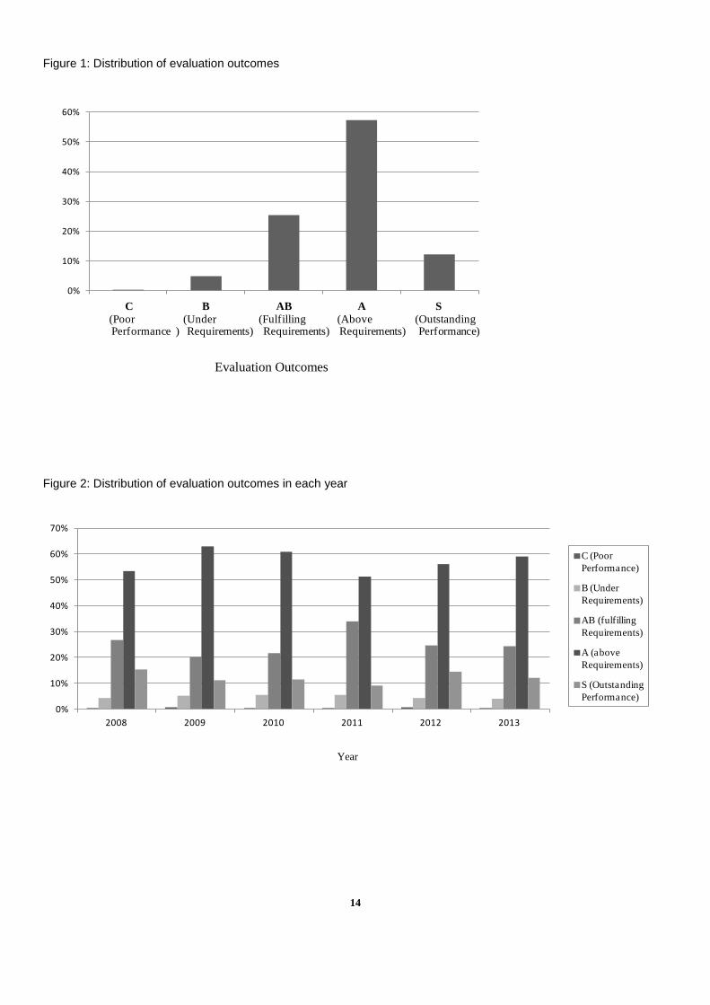
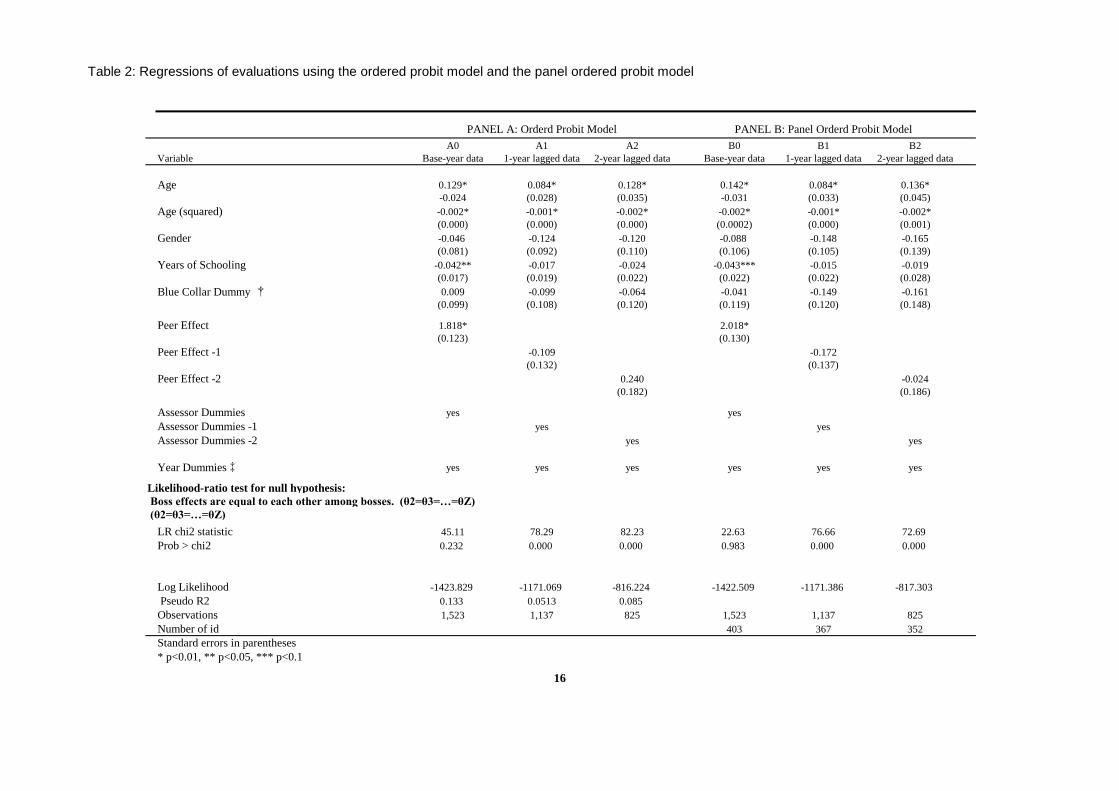