OIW-EX Series of Oil in Water Analyzers - Advanced Sensors · 2.1 - Identifying an OIW EX Series...
80
8 Meadowbank Road, Carrickfergus, BT38 8YF, Northern Ireland www.advancedsensors.co.uk Company Reg. NI 53892 Page 1 of 80 OIW-EX Series of Oil in Water Analyzers Microscopy Handbook Document code: OIW-HBO-0009 Version: EX-009 20 September 2017
Transcript of OIW-EX Series of Oil in Water Analyzers - Advanced Sensors · 2.1 - Identifying an OIW EX Series...

8 Meadowbank Road, Carrickfergus, BT38 8YF, Northern Ireland www.advancedsensors.co.uk
Company Reg. NI 53892 Page 1 of 80
OIW-EX Series of
Oil in Water Analyzers
Microscopy Handbook
Document code: OIW-HBO-0009 Version: EX-009
20 September 2017
8 Meadowbank Road, Carrickfergus, BT38 8YF, Northern Ireland www.advancedsensors.co.uk
Company Reg. NI 53892 Page 2 of 80
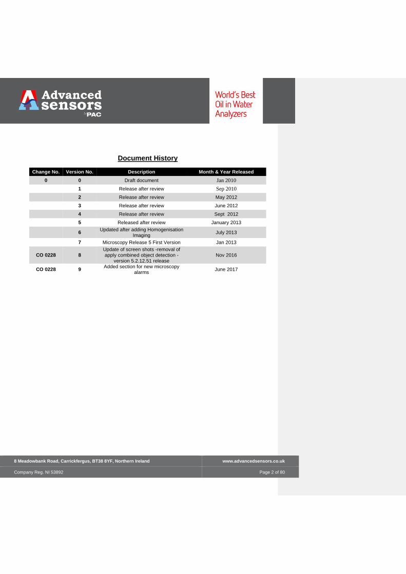
Document History
Change No. Version No. Description Month & Year Released
0 0 Draft document Jan 2010
1 Release after review Sep 2010
2 Release after review May 2012
3 Release after review June 2012
4 Release after review Sept 2012
5 Released after review January 2013
6 Updated after adding Homogenisation
Imaging July 2013
7 Microscopy Release 5 First Version Jan 2013
CO 0228 8 Update of screen shots -removal of apply combined object detection -
version 5.2.12.51 release Nov 2016
CO 0228 9 Added section for new microscopy
alarms June 2017
8 Meadowbank Road, Carrickfergus, BT38 8YF, Northern Ireland www.advancedsensors.co.uk
Company Reg. NI 53892 Page 3 of 80
TABLE OF CONTENTS
OIW-EX SERIES OF ............................................................................................................................................. 1
OIL IN WATER ANALYZERS ........................................................................................................................... 1
MICROSCOPY HANDBOOK ............................................................................................................................. 1
TABLE OF CONTENTS ...................................................................................................................................... 3
SECTION 1 - OIW-EX SERIES - MICROSCOPY HANDBOOK ........................................................................ 5
1.1 - Introduction ................................................................................................................................................................... 6
1.2 Modes of Operation ......................................................................................................................................................... 6
SECTION 2 – MICROSCOPY OVERVIEW ........................................................................................................10
2.1 – Introduction ................................................................................................................................................................ 10
2.1 - Identifying an OIW EX Series Unit with Microscopy Functionality ................................................................................ 11
2.2 - Taking Images for Analysis ........................................................................................................................................... 12 2.2.1 - Imaging Phase in the Measurement Cycle for the EX100M & EX1000M ..................................................................... 13 2.2.2- Imaging Phase in the Measurement Cycle for EX400M ................................................................................................ 14
SECTION 3 - SOFTWARE PANEL DESCRIPTIONS .......................................................................................15
3.1 - Difference between EX400M, EX100M and EX1000M .................................................................................................. 15
3.2 – Switching Between Panels ........................................................................................................................................... 16
3.3 – Colour Coding .............................................................................................................................................................. 17
3.4 – Quick View Panel ......................................................................................................................................................... 18 3.4.1 – Turbidity Measurement ............................................................................................................................................... 19 3.4.2 – Turbidity Indicative Measurement .............................................................................................................................. 20 3.4.3 – Turbidity Attenuation Unit (AU) Measurement ........................................................................................................... 20
8 Meadowbank Road, Carrickfergus, BT38 8YF, Northern Ireland www.advancedsensors.co.uk
Company Reg. NI 53892 Page 4 of 80
3.5 - Size Distribution Panel ................................................................................................................................................. 21 3.5.1-Size Distribution Panel Display Options ......................................................................................................................... 23 3.5.1.1- Left and Right Chart Options ...................................................................................................................................... 24 3.5.1.2 – Plot Type ................................................................................................................................................................... 24 3.5.1.3- Time Period Display Options ...................................................................................................................................... 24
3.6 – The Trending Panel ...................................................................................................................................................... 24 3.6.1 - Trending Panel Display Options .................................................................................................................................... 26 3.6.2 - Trending Panel Quick Menu ......................................................................................................................................... 27
3.7 – The Image Panel .......................................................................................................................................................... 28 3.7.1 Image Panel Open Images .............................................................................................................................................. 29 3.7.2 Image Panel Display Options .......................................................................................................................................... 29 3.7.2.1 - Zooming Options ....................................................................................................................................................... 30 3.7.2.2 – Viewing Options ........................................................................................................................................................ 31 3.7.2.3 – View Type ................................................................................................................................................................. 31
3.8 – Large Image Panel ....................................................................................................................................................... 32
3.9 – Main Top Display Panel ............................................................................................................................................... 33
SECTION 4 - MICROSCOPY CONFIGURATION .............................................................................................34
4.1 – Microscopy Configuration Options .............................................................................................................................. 35
4.2 – Imaging Configuration ................................................................................................................................................. 36
4.3 - Settings ........................................................................................................................................................................ 37 4.3.1 – Shape Factor ................................................................................................................................................................ 38 4.3.2 – Sharpness Factor.......................................................................................................................................................... 38 4.3.3 – Gas Factor .................................................................................................................................................................... 39 4.3.4 – Shape Factor Weights .................................................................................................................................................. 40 4.3.5 – Auto Adjust Shape Factor towards the Fluorescence Value ........................................................................................ 41
4.4 – Calibration ................................................................................................................................................................... 42 4.4.1 – Uniform Calibration ..................................................................................................................................................... 43 4.4.2 – Pixel Calibration Factor ................................................................................................................................................ 43 4.4.3 – Display Raw Image Values ........................................................................................................................................... 43 4.4.4 – Image Calibration ......................................................................................................................................................... 44
4.5 - Object Size ................................................................................................................................................................... 44
4.6 – Alarm Levels ................................................................................................................................................................ 46
4.7 – Density and mg/L ........................................................................................................................................................ 47
4.8 – Advanced .................................................................................................................................................................... 48 4.8.1- Stuck Object Removal .................................................................................................................................................... 49 4.8.2 – Aggressive Size Averaging ............................................................................................................................................ 49 4.8.3 – Flow Valve Control during Static Imaging .................................................................................................................... 49 4.8.4 – Auto Contrast Every 50 Images ................................................................................................................................... 50 4.8.5 – Auto Exposure Every 50 Images .................................................................................................................................. 50

8 Meadowbank Road, Carrickfergus, BT38 8YF, Northern Ireland www.advancedsensors.co.uk
Company Reg. NI 53892 Page 5 of 80
4.8.6 – Image Processing Mode ............................................................................................................................................... 50 4.8.7 – Clean Every nth Image ................................................................................................................................................. 50
4.9 – Homogenisation Imaging ............................................................................................................................................. 51
4.10 – Imaging Test Control ................................................................................................................................................. 52
SECTION 5 – MICROSCOPY MEASUREMENT ALARMS .............................................................................53
SECTION 6 – DATA FILES ..................................................................................................................................62
6.1 – Location....................................................................................................................................................................... 62
6.2 - Data Structure .............................................................................................................................................................. 63
6.3 – File Structure ............................................................................................................................................................... 65
6.4 – File Backup / Removal ................................................................................................................................................. 66
7.1 – Measurements ............................................................................................................................................................ 67 7.1.1 Shape .............................................................................................................................................................................. 67 7.1.2 Size .................................................................................................................................................................................. 71 7.1.3 -Concentration ................................................................................................................................................................ 77
7.2 – Configuration Parameters ........................................................................................................................................... 78
8 – APPENDIX........................................................................................................................................................80
8.1 - OIW-EX Contact Details ................................................................................................................................................ 80
Section 1 - OIW-EX Series - Microscopy Handbook

8 Meadowbank Road, Carrickfergus, BT38 8YF, Northern Ireland www.advancedsensors.co.uk
Company Reg. NI 53892 Page 6 of 80
1.1 - Introduction
The Microscopy Handbook provides information on how to operate an Advanced Sensors Microscopy Analyser
Models EX-100M, EX-400M and EX-1000M. For the EX-100M additional information can be found in User Manual
OIW-HBO-0002 about the operation of the Fluorescence measurement. For the EX-1000M additional information
about the Spectrometer can be found in OIW-HBO-0005.
NOTE: This handbook only covers the operation of the Microscopy. For the basic operation
of Advanced Sensors Ltd OIW-EX-M Series of Oil in Water Analyzer Systems please refer to
OIW-HBO-0002, i.e. the User Handbook.
CAUTION: This manual describes the operation and use of the unit NOT the installation.
Ensure that the unit has been correctly installed in line with the Installation Handbook OIW-
HBO-0001 prior to use.
1.2 Modes of Operation
The OIW-EX Series have been designed with maximum flexibility in mind, enabling them to be configured in a variety of ways to suit different customer requirements.
CAUTION: Should the equipment be used in a manner not specified in this handbook the
sensor may not function correctly and protection provided by the equipment may be
impaired.
CAUTION: No options should be altered without a full understanding of the change being
made.
8 Meadowbank Road, Carrickfergus, BT38 8YF, Northern Ireland www.advancedsensors.co.uk
Company Reg. NI 53892 Page 7 of 80
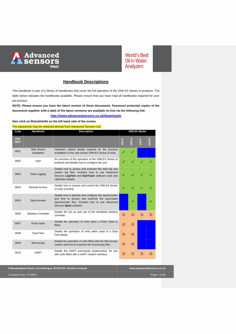
Handbook Descriptions
This handbook is part of a library of handbooks that cover the full operation of the OIW-EX Series of products. The
table below indicates the handbooks available. Please ensure that you have read all handbooks required for your
job function.
NOTE: Please ensure you have the latest version of these documents. Password protected copies of the
documents together with a table of the latest revisions are available on-line via the following link:
http://www.advancedsensors.co.uk/downloads
then click on Documents on the left hand side of the screen.
The passwords may be obtained directly from Advanced Sensors Ltd.
Code Handbook Description OIW EX Model
OIW-HBO-
10
0-S
10
00-S
10
0-P
10
00-P
0001
Side Stream
Installation
Hardware related details required for the physical
installation of the side stream OIW-EX Series of units. ✓ ✓
0002 User An overview of the operation of the OIW-EX Series of
products and details how to configure the unit. ✓ ✓ ✓ ✓
0003 Data Logging
Details how to access and examine the data log and
system log files. Includes how to use Advanced
Sensors LogView and SamTrack software tools and
calibration details.
✓ ✓ ✓ ✓
0004 Remote Access Details how to access and control the OIW-EX Series
of units remotely. ✓ ✓ ✓ ✓
0005 Spectrometer
Details how to operate and configure the spectrometer
and how to access and examine the associated
Spectrometer files. Includes how to use Advanced
Sensors SpAn software.
✓ ✓
0006 Wireless Controller Details the set up and use of the handheld wireless
controller. O O O O
0007 Flush Valve Details the operation of units when a Flush Valve is
fitted. O O
0008 Dual Flow Details the operation of units when used in a Dual
Flow Mode. O O
0009 Microscopy Details the operation of units fitted with the Microscopy
system and how to examine the microscopy files. O O
0010 HART Details the HART commands implemented, for use
with units fitted with a HART modem interface. O O O O

8 Meadowbank Road, Carrickfergus, BT38 8YF, Northern Ireland www.advancedsensors.co.uk
Company Reg. NI 53892 Page 8 of 80
0011 In-Line Probe User An overview of the operation of the OIW-EX P Series
of products and details how to configure the unit. ✓ ✓
0012 In-Line Probe
Installation
Hardware related details required for the physical
installation of the in-line probe OIW-EX P Series of
units. ✓ ✓
0013 MiView Details on how to use the client software for
Microscopy Analysers
Key
✓ Required
O Optional Extra
Not applicable

8 Meadowbank Road, Carrickfergus, BT38 8YF, Northern Ireland www.advancedsensors.co.uk
Company Reg. NI 53892 Page 9 of 80
Symbols used in this handbook
The following symbols are used in this document to indicate special information:
Warning : An instruction that draws attention to the risk of injury or death
Caution: An instruction that draws attention to the risk of damage to the product, process or
surroundings.
Note: Clarification of an instruction or additional information.
Information: Further reference for more detailed information or technical details.
NOTE: Although Warning hazards are related to potential personal injury, and Caution
hazards are associated with material damage, it must be understood that operation of
damaged equipment could lead to personal injury or death.
All Warning and Caution hazards must be complied with.

8 Meadowbank Road, Carrickfergus, BT38 8YF, Northern Ireland www.advancedsensors.co.uk
Company Reg. NI 53892 Page 10 of 80
Section 2 – Microscopy Overview
2.1 – Introduction
The microscopy oil in water analysis system incorporates a camera which periodically takes a series of images and
then analyses those images to identify the size distribution of oil, solids and gas content within the produced water.
If the object is seen as round, then it is identified as oil and if the object is seen as irregular in shape then it is
identified as a solid. This is a recognised method of distinguishing oil from solids. Gas is detected as a round object
with a hole at the centre of the object. By counting oil, solids and gas over a series of images, and knowing the total
area of the images taken, an indication of the ppm of the oil, solids and gas can be obtained.
As the images are analysed the data is displayed immediately on the screen and the user can see the images as
they are taken. In addition, the analysis displayed and the images taken are stored within the OIW EX-M unit,
allowing the user to examine the analysis at a later date and if required perform additional analysis on the images.
To aid in the process of performing additional analysis Advanced Sensors provides a microscopy image software
tool called MiView to help with this task. As with all information provided by Advanced Sensors analysers, users are
free to use other software tools to interrogate the data as the information is stored in simple comma separated text
files, and the images can be viewed with standard tools.
The EX100M and EX100M microscopy system also includes the OIW EX100 and EX1000 fluorescence detection
system for primary oil content measurement.

8 Meadowbank Road, Carrickfergus, BT38 8YF, Northern Ireland www.advancedsensors.co.uk
Company Reg. NI 53892 Page 11 of 80
2.1 - Identifying an OIW EX Series Unit with Microscopy Functionality
The microscopy system is distinguished from the standard OIW-EX Series by the letter M at the end of the model
number i.e. OIW EX400M and OIW EX1000M systems. The number after the M indicates the number of produced
water streams that are being monitored.
The OIW EX400M has only microscopy features. The OIW EX100M/1000M has all the features and functionality of
the OIW EX100M/1000M but with the additional features described in this manual.
The OIW-EX Series software can be distinguished from the OIW-EX-M Series by looking at the software header
box which clearly identifies the unit type, see Figure 1.
Figure 1. OIW EX100M and OIW EX400M software
The following sections will detail the operation of the microscopy system – details will also be provided on the file
format should the user wish to analyse the data with alternative tools.

8 Meadowbank Road, Carrickfergus, BT38 8YF, Northern Ireland www.advancedsensors.co.uk
Company Reg. NI 53892 Page 12 of 80
2.2 - Taking Images for Analysis
Similar to the oil detection system whereby the laser must be on to enable measurement, the microscopy system
requires the lighting system to be on to take and analyse images, therefore the analyser will not operate when the
measurement cycle is in the stopped position.
There is a facility to take a single image while the measurement cycle is stopped, but this will not form part of the
daily trending analysis.

8 Meadowbank Road, Carrickfergus, BT38 8YF, Northern Ireland www.advancedsensors.co.uk
Company Reg. NI 53892 Page 13 of 80
2.2.1 - Imaging Phase in the Measurement Cycle for the EX100M & EX1000M
Imaging is done before the homogenisation process with either the valve closed in Static Mode or with the valve
opened in Flow Mode. The differences in these two modes are described in more detail in section 6.2.
Figure 2. OIW-EX100M and 1000M Measurement Cycle
The image processing may continue after the system has moved on to the homogenisation and other phases – the
images and microscopy data will be displayed as soon as the information becomes available.

8 Meadowbank Road, Carrickfergus, BT38 8YF, Northern Ireland www.advancedsensors.co.uk
Company Reg. NI 53892 Page 14 of 80
2.2.2- Imaging Phase in the Measurement Cycle for EX400M
The schedule for the EX400M is cleaning of the optical components using the ultra sonics, followed by the
imaging phase. Cleaning happens with the flow open. Images can be set to be in Flow Mode (that is with
produced water flowing through the system during imaging) or image Static Mode (the valve is closed and the
produced water remains static in the chamber during sampling).
8 Meadowbank Road, Carrickfergus, BT38 8YF, Northern Ireland www.advancedsensors.co.uk
Company Reg. NI 53892 Page 15 of 80
Section 3 - Software Panel Descriptions
3.1 - Difference between EX400M, EX100M and EX1000M
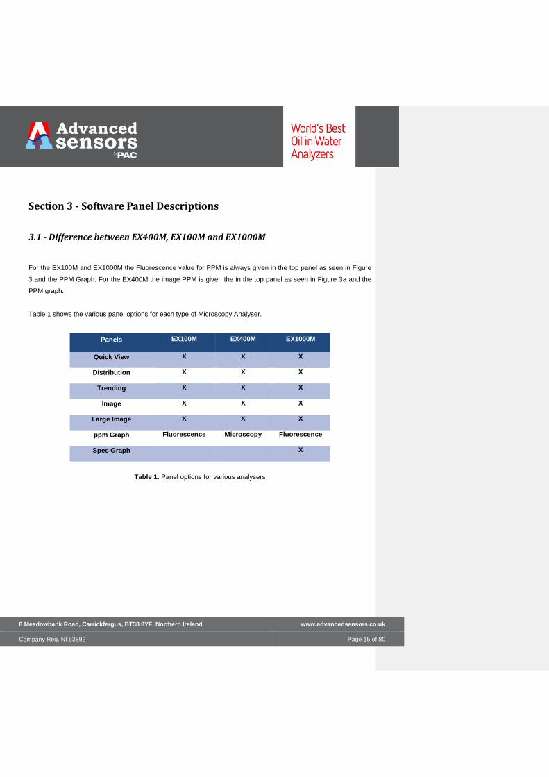
For the EX100M and EX1000M the Fluorescence value for PPM is always given in the top panel as seen in Figure
3 and the PPM Graph. For the EX400M the image PPM is given the in the top panel as seen in Figure 3a and the
PPM graph.
Table 1 shows the various panel options for each type of Microscopy Analyser.
Panels EX100M EX400M EX1000M
Quick View X X X
Distribution X X X
Trending X X X
Image X X X
Large Image X X X
ppm Graph Fluorescence Microscopy Fluorescence
Spec Graph X
Table 1. Panel options for various analysers
8 Meadowbank Road, Carrickfergus, BT38 8YF, Northern Ireland www.advancedsensors.co.uk
Company Reg. NI 53892 Page 16 of 80
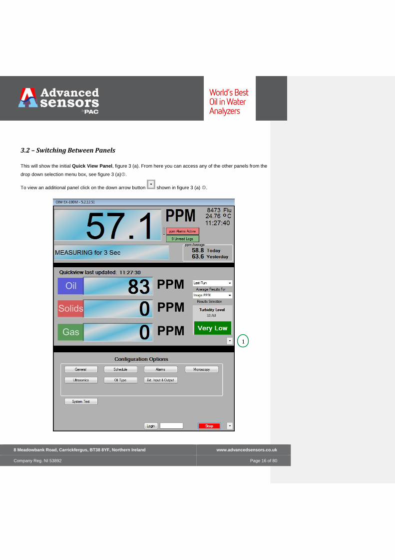
3.2 – Switching Between Panels
This will show the initial Quick View Panel, figure 3 (a). From here you can access any of the other panels from the
drop down selection menu box, see figure 3 (a).
To view an additional panel click on the down arrow button shown in figure 3 (a) .
1

8 Meadowbank Road, Carrickfergus, BT38 8YF, Northern Ireland www.advancedsensors.co.uk
Company Reg. NI 53892 Page 17 of 80
(a)
(b)
Figure 3. Switching Panels
3.3 – Colour Coding
All screens follow a colour code convention for displaying the data. Oil droplet data is displayed in blue, solids data
is displayed in red and gas in green. That is, bar charts, graphs and markings on images in blue represent oil
droplets data, bar charts, graphs and markings on images in red represent solids data and bar charts, graphs and
markings on images in green represent gas data.
2
8 Meadowbank Road, Carrickfergus, BT38 8YF, Northern Ireland www.advancedsensors.co.uk
Company Reg. NI 53892 Page 18 of 80
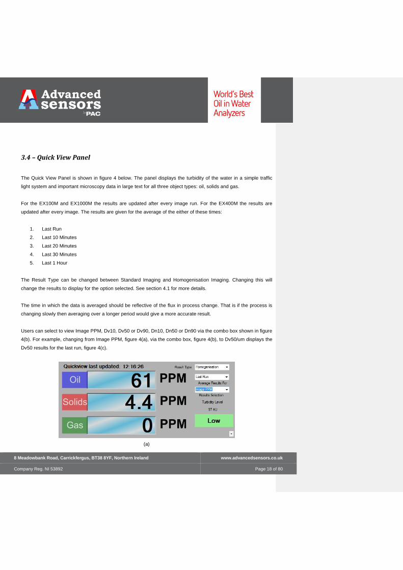
3.4 – Quick View Panel
The Quick View Panel is shown in figure 4 below. The panel displays the turbidity of the water in a simple traffic
light system and important microscopy data in large text for all three object types: oil, solids and gas.
For the EX100M and EX1000M the results are updated after every image run. For the EX400M the results are
updated after every image. The results are given for the average of the either of these times:
1. Last Run
2. Last 10 Minutes
3. Last 20 Minutes
4. Last 30 Minutes
5. Last 1 Hour
The Result Type can be changed between Standard Imaging and Homogenisation Imaging. Changing this will
change the results to display for the option selected. See section 4.1 for more details.
The time in which the data is averaged should be reflective of the flux in process change. That is if the process is
changing slowly then averaging over a longer period would give a more accurate result.
Users can select to view Image PPM, Dv10, Dv50 or Dv90, Dn10, Dn50 or Dn90 via the combo box shown in figure
4(b). For example, changing from Image PPM, figure 4(a), via the combo box, figure 4(b), to Dv50/um displays the
Dv50 results for the last run, figure 4(c).
(a)

8 Meadowbank Road, Carrickfergus, BT38 8YF, Northern Ireland www.advancedsensors.co.uk
Company Reg. NI 53892 Page 19 of 80
(b)
(c)
Figure 4. The Quick View Panel
When homogenisation and flowing image are both enabled, the user can select on the dialog between viewing the
results for either the flowing or homogenisation periods.
3.4.1 – Turbidity Measurement
Microscopy system reports the level of turbidity in a simple traffic colour code as well as Attention Units display in
Quick View Panel. The turbidity measurement is taken from the transmission of light through the sample in the
chamber.
8 Meadowbank Road, Carrickfergus, BT38 8YF, Northern Ireland www.advancedsensors.co.uk
Company Reg. NI 53892 Page 20 of 80
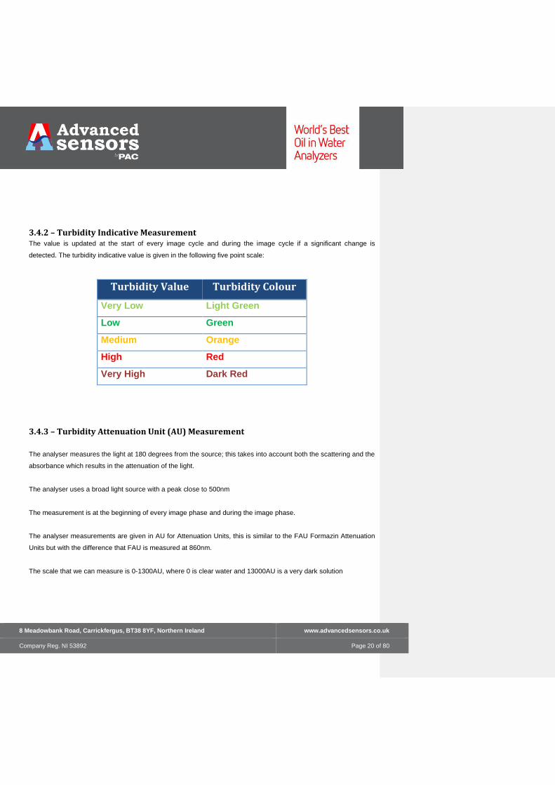
3.4.2 – Turbidity Indicative Measurement The value is updated at the start of every image cycle and during the image cycle if a significant change is
detected. The turbidity indicative value is given in the following five point scale:
Turbidity Value Turbidity Colour
Very Low Light Green
Low Green
Medium Orange
High Red
Very High Dark Red
3.4.3 – Turbidity Attenuation Unit (AU) Measurement
The analyser measures the light at 180 degrees from the source; this takes into account both the scattering and the
absorbance which results in the attenuation of the light.
The analyser uses a broad light source with a peak close to 500nm
The measurement is at the beginning of every image phase and during the image phase.
The analyser measurements are given in AU for Attenuation Units, this is similar to the FAU Formazin Attenuation
Units but with the difference that FAU is measured at 860nm.
The scale that we can measure is 0-1300AU, where 0 is clear water and 13000AU is a very dark solution

8 Meadowbank Road, Carrickfergus, BT38 8YF, Northern Ireland www.advancedsensors.co.uk
Company Reg. NI 53892 Page 21 of 80
3.5 - Size Distribution Panel
The Size Distribution Panel is shown below, figure 5. This panel displays two charts; for either a combination of oil
droplets (blue chart), solids (red chart) and gas (green chart). To view the different object types see section
3.5.1.
1 1
2 2
3

8 Meadowbank Road, Carrickfergus, BT38 8YF, Northern Ireland www.advancedsensors.co.uk
Company Reg. NI 53892 Page 22 of 80
Figure 5. The Image Distribution Panel
There are three types of graphs that can be displayed:
• Distribution-Figure 5
The distribution is the frequency percentage of data given for 40 point intervals between the maximum and
minimum values of the x-axis. The frequency percentage values are given on the left hand of the charts in
figure 6.
• Cumulative- Figure 5
The cumulative is the sum of all frequency percentage data less than the value on the x-axis. The
cumulative frequency percentage values are given on the right hand of the charts in figure 6.
• Distribution and Cumulative- Figure 5
This displays both the distribution and cumulative charts.
A variety of data is displayed below each chart and includes:
• Dv10 -the particle size below which 10 per cent of the volume of material is found.
• Dv50 –the median particle size, the particle size below which 50 per cent of the volume of material is
found.
• Dv90 –the particle size below which 90 per cent of the volume of material is found.
• The total number of images used for the chart data is displayed at the bottom right of the dialog.
When homogenisation and flowing image are both enabled, the user can select on the dialog between viewing the
results for either the flowing or homogenisation periods.
8 Meadowbank Road, Carrickfergus, BT38 8YF, Northern Ireland www.advancedsensors.co.uk
Company Reg. NI 53892 Page 23 of 80
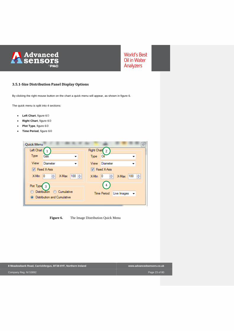
3.5.1-Size Distribution Panel Display Options
By clicking the right mouse button on the chart a quick menu will appear, as shown in figure 6.
The quick menu is split into 4 sections:
• Left Chart, figure 6
• Right Chart, figure 6
• Plot Type, figure 6
• Time Period, figure 6
Figure 6. The Image Distribution Quick Menu
1
2
4
3

8 Meadowbank Road, Carrickfergus, BT38 8YF, Northern Ireland www.advancedsensors.co.uk
Company Reg. NI 53892 Page 24 of 80
3.5.1.1- Left and Right Chart Options
Type:
Changing the type will change if oil, solids or gas data is displayed in the left or right chart.
View:
Allows the chart to display Area, Volume, Diameter or Shape distribution on the left or right charts.
Fixed X-Axis, X-Min and X-Max:
The size axis (x-axis) can also be configured to a fixed range – in which case the minimum and maximum range
can be set, or full range – in which case the graph will dynamically change the x-axis to display all objects detected.
3.5.1.2 – Plot Type
Changing the plot type will change the type of plot that is displayed on both graphs.
3.5.1.3- Time Period Display Options
This allows the user to display either the analysis of the Live Data or today’s data.
3.6 – The Trending Panel
The Trending panel is shown below in figure 7; this panel displays up to four plots for live timing and two for other
time periods.
The top chart in figure 7 is the Dv50 value for Live Image time period. In this mode there are four lines displayed.
The light blue line represents the actual Dv50 values of oil droplets for each image, while the heavy blue line
represents the average DV50 value of oil droplets for all the images in the run. Similarly, the light red line
represents the actual Dv50 values of solids for each image, while the heavy red line represents the average Dv50
values of solids for images in the run.
The total number of images used for the chart data is displayed at the top right of the trending dialog.

8 Meadowbank Road, Carrickfergus, BT38 8YF, Northern Ireland www.advancedsensors.co.uk
Company Reg. NI 53892 Page 25 of 80
Figure 7. The Trending Panel
When homogenisation and flowing image are both enabled, the user can select on the dialog between viewing the
results for either the flowing or homogenisation periods.

8 Meadowbank Road, Carrickfergus, BT38 8YF, Northern Ireland www.advancedsensors.co.uk
Company Reg. NI 53892 Page 26 of 80
3.6.1 - Trending Panel Display Options
The Chart Type can be set to any of the options shown.
PPM
mgl
Area
Volume
Dv10
Dv50
Dv90
Dn10
Dn50
Dn90
Shape
Number of Objects
Turbidity
Temperature
Circularity
Aspect Ratio
Convexity
Elongation
Projected Circle
Sharpness
Feret Diameter
Length
Width

8 Meadowbank Road, Carrickfergus, BT38 8YF, Northern Ireland www.advancedsensors.co.uk
Company Reg. NI 53892 Page 27 of 80
3.6.2 - Trending Panel Quick Menu
By clicking the right mouse button on the chart a quick menu will appear, as shown in figure 8.
Figure 8. The Trending Panel Quick Menu
The Y-axis position can be set to a fixed value or updated dynamically by checking on the Fixed Y-Axis check box.
The minimum and maximum Y-Axis values for the fixed graph are set by changing the Y-Min and Y-Max values.
Changing the View type will change which object data is displayed in the chart and table. The combinations are:
Oil + Solids
Oil + Gas
Solids + Gas
Note: if the Time Period is set to anything other than the Live Image then the light red and blue lines that represent
the live information are not displayed.

8 Meadowbank Road, Carrickfergus, BT38 8YF, Northern Ireland www.advancedsensors.co.uk
Company Reg. NI 53892 Page 28 of 80
3.7 – The Image Panel
The Image Panel displays the last image taken and the analysis of that image. This can be seen below, figure 9.
Detected oil droplets are coloured in blue, detected solids in red and gas as green. To help identify objects yellow
grid lines are displayed over the image. The yellow text in the centre of each grid line highlights the distance in µm
between each grid line, and the markings on the gridline indicate the distance in µm from the zero origin of the
image ([0,0] in the lower left corner). The date and time of the image displayed are shown next to the image.
Figure 9. The Image Panel

8 Meadowbank Road, Carrickfergus, BT38 8YF, Northern Ireland www.advancedsensors.co.uk
Company Reg. NI 53892 Page 29 of 80
3.7.1 Image Panel Open Images
An image previously saved can be opened and viewed on the image panel using the Open Image button.
Processed images file names begin with ‘OIWImageProcessed’ whereas the non processed images file names
start with ‘OIWImage’. See section 5 for information on File Structure.
3.7.2 Image Panel Display Options
The default display for the image panel is to show the processed image with detected oil droplets coloured in blue
and detected solids in red as shown above.
By clicking the right mouse button on the image a quick menu will appear, as shown below, figure 10.
Figure 10. Image Panel Display Options
This menu has two sections: Zooming Options and Viewing Options.

8 Meadowbank Road, Carrickfergus, BT38 8YF, Northern Ireland www.advancedsensors.co.uk
Company Reg. NI 53892 Page 30 of 80
3.7.2.1 - Zooming Options
To zoom in on an area of an image select the “To Zoom in Click on Image” radio button, then click on an area of
the image you want to view more closely. This option will revert back to the Pan Image option allowing the image to
be panned around the image window. To zoom in further simply click on the “To Zoom in Click on Image” option
again. As zooming in takes place the yellow distance between grid lines will be updated as will the position from
origin.
Figure 11 below shows an example of an object that has been zoomed in on.
Figure 11. Example of Zooming in on an Image

8 Meadowbank Road, Carrickfergus, BT38 8YF, Northern Ireland www.advancedsensors.co.uk
Company Reg. NI 53892 Page 31 of 80
3.7.2.2 – Viewing Options
As mentioned the default display for the image panel is to show the processed image with detected oil droplets
coloured in blue, detected solids in red and gas as green. The viewing options allow the image to be displayed
with only the oil droplets highlighted, only the solids highlighted, only the gas highlighted, with nothing highlighted
(the image with no markings), or with all oil droplets, solids and gas shown.
Figure 12 shows the differences between highlighting solids and selecting unmarked.
Figure 12. Examples of Image View Options
3.7.2.3 – View Type
Changing the view type will change the object type that is displayed in the image panels table.
1
2

8 Meadowbank Road, Carrickfergus, BT38 8YF, Northern Ireland www.advancedsensors.co.uk
Company Reg. NI 53892 Page 32 of 80
3.8 – Large Image Panel
The Large Image Panel includes all the features of the Image Panel in section 3.7 minus the results table.
Figure 13. Large Image Panel

8 Meadowbank Road, Carrickfergus, BT38 8YF, Northern Ireland www.advancedsensors.co.uk
Company Reg. NI 53892 Page 33 of 80
3.9 – Main Top Display Panel
Figure 17 shows the main display at the top of the software.
Figure 17. Main Display
Descriptions of areas in Main Display Figure 17
1. For EX1000M and EX100M PPM or mg/L value is related to the fluorescence measurement. For further
details for these models please refer to OIW-HBO-002 User Manual. For the EX400M the value displayed
is related to the object selected in the Main Display option in the Microscopy Configuration. The object type
is displayed at the top of area 2.
2. Either the object type (EX400M) or the raw fluorescence value is displayed at the top of area 2.
The temperature of the measurement chamber is then displayed
3. The alarms for the system are displayed here.
4. Displays the current cycle status. For information please refer to OIW-HBO-002.
5. The average value of PPM for today and yesterday. For EX1000M and EX100M the value is related to the
fluorescence measurement. For further details for these models please refer to OIW-HBO-002 User
Manual. For the EX400M the value displayed is related to the object selected in the Main Display option in
the Microscopy Configuration. The Object type is displayed at the top of area 2.
1
2
3
4
5

8 Meadowbank Road, Carrickfergus, BT38 8YF, Northern Ireland www.advancedsensors.co.uk
Company Reg. NI 53892 Page 34 of 80
Section 4 - Microscopy Configuration
The microscopy configuration options button (Figure 18) can be found under the Configuration Options in the
bottom control (Figure 18). You will need to log in to make any changes. Note: this button will only be visible for
OIW-EX-M Series users.
Figure 18. Microscopy Configuration Button

8 Meadowbank Road, Carrickfergus, BT38 8YF, Northern Ireland www.advancedsensors.co.uk
Company Reg. NI 53892 Page 35 of 80
4.1 – Microscopy Configuration Options
Note: Some options can only be changed if the cycle has been stopped
The configuration is split into a number of tabs (as seen in figure 19) which will be described in the following
sections.
Figure 19. Microscopy Configuration Window
The controls at the bottom of the panel have the following functions:
• Close button will close the microscopy configuration tab
• Load Configuration button can be used to load a new configuration file which will update microscopy
configuration value. These can be generated using MiView Batch and Image Reprocessing Application
• Export Configuration button can be used to save a new configuration file which can be loaded onto the
MiView Batch Image Reprocessing Application

8 Meadowbank Road, Carrickfergus, BT38 8YF, Northern Ireland www.advancedsensors.co.uk
Company Reg. NI 53892 Page 36 of 80
4.2 – Imaging Configuration
The Imaging Configuration shown in Figure 19 is used to set configuration options related to the imaging.
• Imaging Mode is described in section 6.2,
• Image Sampling controls how many images should be taken during each imaging phase of the
measurement cycle, and the time interval between each image.
• No. Images to be Saved is the number of images that will be saved to the during each image cycle.
• Main Display (EX400M only) changes what object type is displayed in the PPM Graph and Main Display.
• Imaging Schedule can set the imaging to take place with and without homogenisation. Homogenisation
will break up the oil droplets into much smaller particle sizes, so do not used the result from this phase for
measurement of oil droplet size. Homogenisation imaging can be used to remove oil that has coated solids.

8 Meadowbank Road, Carrickfergus, BT38 8YF, Northern Ireland www.advancedsensors.co.uk
Company Reg. NI 53892 Page 37 of 80
4.3 - Settings
This section controls the settings for the detection algorithm. It is important to understand that any changes made
to these settings will affect the PPM reading derived from the image. For this reason any changes made may
require a change to the Oil, Solids and Gas Gain (see section6).
(a)
(b)
Figure 20. Settings tab for (a) EX400M and (b) EX100M/1000M

8 Meadowbank Road, Carrickfergus, BT38 8YF, Northern Ireland www.advancedsensors.co.uk
Company Reg. NI 53892 Page 38 of 80
4.3.1 – Shape Factor
As mentioned previously, the image analysis distinguishes oil droplets from solids by assessing the shape of
objects found in the image. If the object is seen as round then it is identified as oil and if the object is seen as
irregular in shape then it is identified as a solid. The degree to which an identified object is categorised as an oil
droplet is based on the Shape Factor setting.
The higher this setting is the ‘rounder’ the oil droplet must be to be considered as an oil droplet. A shape factor of 1
means completely round object. Anything not categorised as round will be marked as a solid. Figure 21 below
provides simplified examples of roundness.
Figure 21. Roundness Factor Objects
4.3.2 – Sharpness Factor
Images which are out of the main focal plane will be blurred (not sharp) and can appear larger than they actually
are. This factor determines which objects will be considered as ‘in focus’ and should be considered as detected
objects, and which objects should be ignored as they will be inaccurately measured if identified as an object.
The higher the factor, the sharper an object must be to be detected.

8 Meadowbank Road, Carrickfergus, BT38 8YF, Northern Ireland www.advancedsensors.co.uk
Company Reg. NI 53892 Page 39 of 80
Figure 22. Sharpness Factor Objects
Using Figure 22 as an example, setting the Sharpness Factor to 1.00 will detect only objects fully in focus: object
1. Objects 2 and 3 will not be detected as they are blurred (out of the focal plane). Setting the Sharpness Factor to
0.50 will detect objects 1 and 2, but will ignore object 3 as it is too blurred.
4.3.3 – Gas Factor
Gas bubbles will differ from oil droplets as they will have a clear centre. This factor controls the white to black ratio
of the detected object and allows the detection algorithm to ignore gas bubbles to improve the accuracy of the oil
measurement system detection.
Figure 23. Gas Factor Objects
Using Figure 23 as an example, setting the Gas Factor to 0 (zero) will detect any round object with an inner white
portion as a gas (all objects). Setting the Gas Factor to 20 will only detect objects below 20% clear as gas i.e.
objects 2 and 3; object 1 will be detected as an oil droplet. Setting the Gas Factor to 60 in this example will not

8 Meadowbank Road, Carrickfergus, BT38 8YF, Northern Ireland www.advancedsensors.co.uk
Company Reg. NI 53892 Page 40 of 80
detect any object below 60% clear as gas and all objects will be detected as oil droplets i.e. only objects with
greater than 60% clear will be seen as gas.
4.3.4 – Shape Factor Weights
The shape factor is made up of a number of different properties of the object. These properties can be weighted in
order to represent the differences between oil and solids objects in the water. That is for example when solid
objects are round the convexity and greyscale weights can be increased to better detect round solids.
Roundness Weight
The roundness is related to the objects perimeter and area, the larger the perimeter to the area the lower the
roundness value will be.
Aspect Ratio Weight
The aspect ratio is related to the ratio of the objects width against height, see section 6.1.1 Shape.
Percentage of Projected Circle Weight
Percentage of the edge of the object that falls within +-10% of a projected circle from the centre of mass of the
object. This property is good at differentiating between oil and solid objects, see section 6.1.1 Shape.
Circularity Weight
The Circularity is related to the ratio of the projected perimeter from the objects area to its actual perimeter, see
section 6.1.1 Shape.
Convexity Weight
Convexity is an indication of how rough the particle is, see section 6.1.1 Shape.
Greyscale Weight
Greyscale Variation is an indication of how textured the object is. In general oil objects will have very little texture
and solids will have some texture in the object

8 Meadowbank Road, Carrickfergus, BT38 8YF, Northern Ireland www.advancedsensors.co.uk
Company Reg. NI 53892 Page 41 of 80
4.3.5 – Auto Adjust Shape Factor towards the Fluorescence Value
When the Auto Adjust Shape Factor towards the Fluorescence Value check box is ticked in figure 20(b) the shape
factor will be adjusted so that the microscopy ppm and the fluorescence ppm become similar. The min and max
auto shape factor are boundary conditions that shape factor must remain in.
This option should only be used when the differences in shape between oil and solids are very similar. The
differences in the min and max should also be set no greater than 0.2.

8 Meadowbank Road, Carrickfergus, BT38 8YF, Northern Ireland www.advancedsensors.co.uk
Company Reg. NI 53892 Page 42 of 80
4.4 – Calibration
(a)
(b)
Figure 24. Calibration Tab for (a) EX400M and (b) EX100M/1000M

8 Meadowbank Road, Carrickfergus, BT38 8YF, Northern Ireland www.advancedsensors.co.uk
Company Reg. NI 53892 Page 43 of 80
4.4.1 – Uniform Calibration
A uniform calibration is used to correct non-uniformities in the image. This is done periodically in case, for example,
the Analyser receives a physical knock that may move the camera slightly.
By ticking “Perform Uniform Image On Next Cycle” a uniform image will be processed before the next Image Cycle.
4.4.2 – Pixel Calibration Factor
The Pixel Calibration Factor is the size each pixel in the image represents in um. That is if the factor is 0.4 then 1
pixel is 0.4µm. 40µm would give 100 pixels in length. This can only be adjusted by an Advanced Sensors
Engineer.
4.4.3 – Display Raw Image Values
By checking the Display Raw Image Values check box the raw image values are sent to the quick view control for
each of the object types, as seen in figure 25. The raw image value is used for calibration of the microscopy object
concentration.
Figure 25. Calibration Tab for (a) EX400M and (b) EX100M/1000M

8 Meadowbank Road, Carrickfergus, BT38 8YF, Northern Ireland www.advancedsensors.co.uk
Company Reg. NI 53892 Page 44 of 80
4.4.4 – Image Calibration
For the EX100M and EX1000M the PPM reading obtained from the image is secondary value for Oil PPM and it is
important to understand that for this system the fluorescence PPM is the primary value for Oil PPM.
The seven values A, B, C, D, m, c and intercept are the parameters for the calibration curve for the microscopy
system.
The load calibration file can be used to update the calibration values.
For EX100M and EX1000M
The Imaging PPM can auto calibrate itself to the fluorescence measurement by checking the Auto Calibration
check box. This has the effect of the system adjusting the Oil Gain to match the Fluorescence PPM
By checking Link Auto Calibration to Solids + Gas the multiplication factor used to adjust the Oil Gain is applied
to the Solids and Gas Gain. This should be unselected once the oil calibration is complete.
For EX400M
The Oil, Solids and Gas Gain can be adjusted separately. This may be important when calibrating for example the
Solids PPM against the lab measurement.
4.5 - Object Size
Object Size Tab Figure 26 allows the user to edit the detection size for oil, solids and gas.
For example, if the max diameter for oil was 100µm and min diameter was 10µm the following would happen:
Oil droplet size 112µm would not be detected and oil droplet size 6µm would not be detected, whereas any oil
droplets between 10 and 100µm, such as an oil droplet of 30µm, would be detected.
Setting the size of the Oil, Solids and Gas objects can help reduce any false-positive objects being picked up. That
is, if we know that the oil objects in the system range between 1 and 20µm, then we could consider objects that are
round, and bigger than 20µm, to be either solids or gas objects.

8 Meadowbank Road, Carrickfergus, BT38 8YF, Northern Ireland www.advancedsensors.co.uk
Company Reg. NI 53892 Page 45 of 80
If a possible oil object is bigger than the set Max Value, the object can be considered as:
• No Object if the If > than Max Leave Empty is checked
• Solid if the If > than Max set as Solid is checked
• Gas if the If > than Max set as Gas is checked
Figure 26. Object Size Tab

8 Meadowbank Road, Carrickfergus, BT38 8YF, Northern Ireland www.advancedsensors.co.uk
Company Reg. NI 53892 Page 46 of 80
4.6 – Alarm Levels
The Imaging Alarm is configured by the Alarm Levels tab.
The user can set the fluorescence to go out of range if the Turbidity is very high by checking on Set PPM to Out of
Range when Turbidity is very high to. The turbidity very high PPM value can be set by the user.
Figure 27. Warning Level Tab
8 Meadowbank Road, Carrickfergus, BT38 8YF, Northern Ireland www.advancedsensors.co.uk
Company Reg. NI 53892 Page 47 of 80
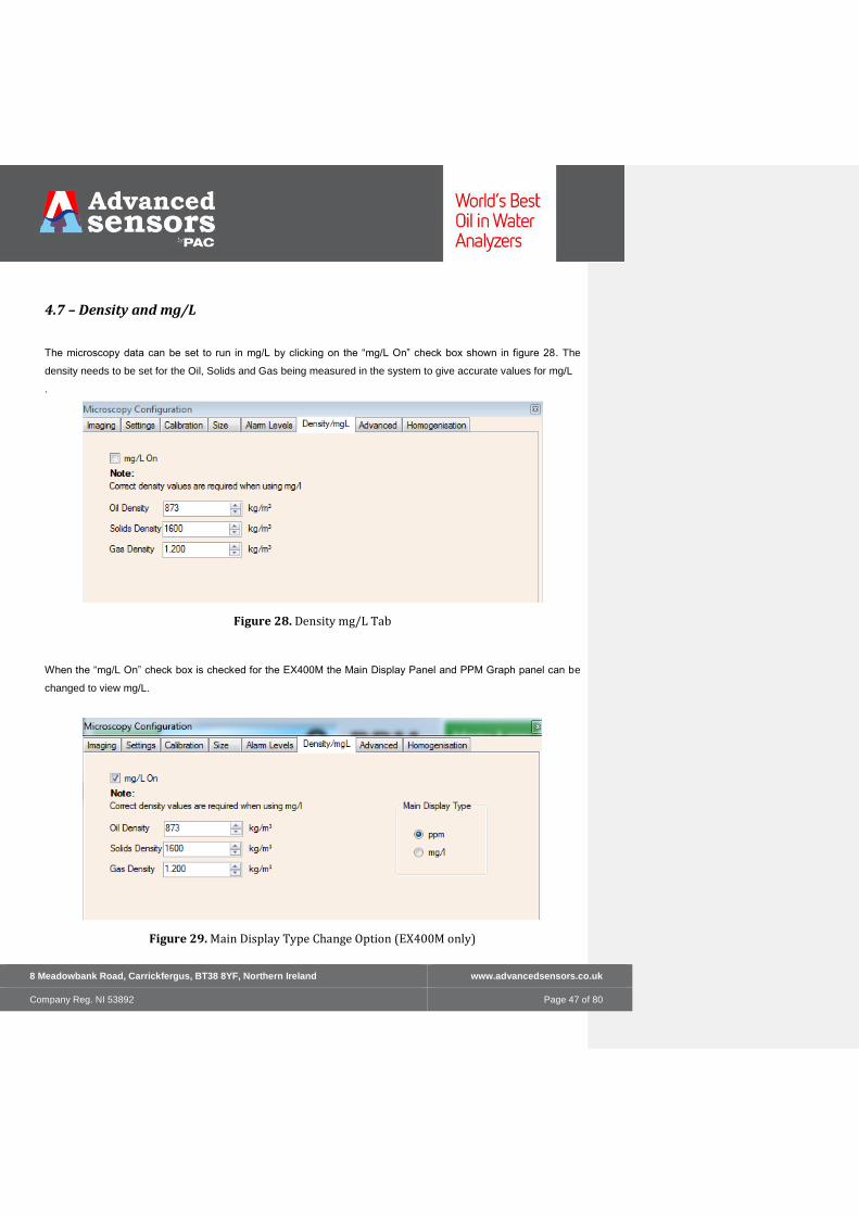
4.7 – Density and mg/L
The microscopy data can be set to run in mg/L by clicking on the “mg/L On” check box shown in figure 28. The
density needs to be set for the Oil, Solids and Gas being measured in the system to give accurate values for mg/L
.
Figure 28. Density mg/L Tab
When the “mg/L On” check box is checked for the EX400M the Main Display Panel and PPM Graph panel can be
changed to view mg/L.
Figure 29. Main Display Type Change Option (EX400M only)

8 Meadowbank Road, Carrickfergus, BT38 8YF, Northern Ireland www.advancedsensors.co.uk
Company Reg. NI 53892 Page 48 of 80
4.8 – Advanced
Features in this section should be adjusted with care. Advanced Sensors recommends the following settings
Figure 30. Advanced Microscopy Configuration settings

8 Meadowbank Road, Carrickfergus, BT38 8YF, Northern Ireland www.advancedsensors.co.uk
Company Reg. NI 53892 Page 49 of 80
4.8.1- Stuck Object Removal
Objects that stick to the optical window will appear in the same place in multiple images causing the object to be
counted over and over again. With the Advanced Sensors ultra sonic cleaning technology the probability of objects
being stuck on the window is low.
By checking the Stuck Objects Removal check box the object will only be counted once and then ignored.
4.8.2 – Aggressive Size Averaging
The size in terms of the distribution volumetric is calculated for all the objects in all the images in the run.
This value is then averaged over all the runs in the time period of observation.
The averaging of the distribution volumetric can be average over every 50 images instead. This will reduce the
effect of large particles on the average value
4.8.3 – Flow Valve Control during Static Imaging
When in a static image mode to reduce the affect of oil and solid objects settling over the imaging period the flow
valve can be opened every 50 images of the image cycle.
The delay between the flow valve closing again and the imaging taking place can also be set. This is important as
closing the valve in a high pressure line can cause a quick rush of gas.
The time the valve is opened for can be set and should reflect the flow rate of the line.

8 Meadowbank Road, Carrickfergus, BT38 8YF, Northern Ireland www.advancedsensors.co.uk
Company Reg. NI 53892 Page 50 of 80
4.8.4 – Auto Contrast Every 50 Images
Enables the image processing to perform an auto contrast after every 50 images. Normally this is done at the
beginning of each cycle. May be useful if the concentration or turbidity of the water changes rapidly over time.
By default, this should be selected.
4.8.5 – Auto Exposure Every 50 Images
Enables the image processing to perform an auto exposure after every 50 images. Normally this is done at the
beginning of each cycle. May be useful if the concentration or turbidity of the water changes rapidly over time.
By default, this should be selected.
4.8.6 – Image Processing Mode
The speed of the image processing can be adjusted for faster processing, although the sensitivity (that is the ability
to pick up all the objects in the image) is sacrificed.
By default, this should be set to sensitive.
4.8.7 – Clean Every nth Image
Allows the analyser to perform a cleaning phase after n number of images. May be useful in high gas or
concentration.

8 Meadowbank Road, Carrickfergus, BT38 8YF, Northern Ireland www.advancedsensors.co.uk
Company Reg. NI 53892 Page 51 of 80
4.9 – Homogenisation Imaging
The settings for the homogenisation image configuration are split into two sections:
Homogenisation Settings
• Power the power level for the ultrasonic cleaning
• PWM the length of the ultrasonic pulse in time
• PWM Ratio the ratio the ultrasonics is on/off
• Time On the total length of time of the ultrasonic cleaning phase
Image Sampling
Controls how many images should be taken during each imaging phase of the measurement cycle, and the time
interval between each image.
Figure 31. Homogenisation Imaging Options

8 Meadowbank Road, Carrickfergus, BT38 8YF, Northern Ireland www.advancedsensors.co.uk
Company Reg. NI 53892 Page 52 of 80
4.10 – Imaging Test Control
By clicking on the System Test button on the configuration panel and then on the Microscopy Tab you can get
access to control the Light and take images manually.
Figure 32. Microscopy System Test

8 Meadowbank Road, Carrickfergus, BT38 8YF, Northern Ireland www.advancedsensors.co.uk
Company Reg. NI 53892 Page 53 of 80
Section 5 – Microscopy Measurement Alarms
Configurable microscopy measurement alarms allow the user to set lower and upper measurement threshold
alarms, allocate alarm limits to relays and configure alarm timings. All alarms are recorded in the system logs for
complete traceability.
Microscopy Measurement Alarms
INFORMATION: Measurement alarms correspond to the user defined measurement unit.
Therefore measurement alarms will be displayed in ppm, ppb, % or mg/l units according to
user configuration.
Microscopy Measurement alarms provide the user with warnings to indicate measurement values have exceeded
either one of the set threshold limits. Figure 31 below of the ‘Measurement Alarms’ menu shows the menu options
and the ‘Alarm Settings’ box in the ‘Configurations Setting’ display area. Measurement alarm configuration options
(when enabled or disabled) are displayed in the ‘Configurations Setting’ display area for quick reference.
Figure 33: Measurement Alarms configuration menu and configuration settings display area. *Example for illustration only actual screen may vary with alarm type.
The ‘Enable Alarm Threshold 1’ box must be ticked to enable and edit this feature. If a second limit is required then
the ‘Enable Alarm Threshold 2’ box can be selected (note: ‘Enable Alarm Threshold 1’ must be enabled first before
the second alarm threshold can be selected). Limits are set using the numerical up / down arrows in the threshold
box and displayed in the ‘Configurations Setting’ display area as shown above in Figure 31. Relays can be
allocated to trigger when alarm threshold 1 is crossed. The user can select a relay, all or none from the drop-down
list at the bottom of the menu. The dry contact relay can, for example, activate an audible alarm in the control room,

8 Meadowbank Road, Carrickfergus, BT38 8YF, Northern Ireland www.advancedsensors.co.uk
Company Reg. NI 53892 Page 54 of 80
open/close a valve to reroute the process flow or any other user requirement (set up at the time of installation) to
indicate an alarm status.
If an alarm threshold is crossed the user can configure a time limit, ‘Alarm Persistence’, before an alarm is raised to
compensate for temporary out of threshold variations in measurement values. The measured value must then
exceed the thresholds for the specified time before an alarm is raised. In Figure 33, the ‘Alarm Persistence’ time is
selected using the numerical up / down arrows, to a maximum time of 120 seconds. The selected persistence time
is then displayed in the ‘Configurations Setting’ display area as shown in Figure 33. A pending alarm message, in
yellow, will be displayed on screen, as well as the alarm panel, during the persistence period until the time is
exceeded when an alarm is issued, shown in Figure 34. Otherwise if the measurement returns to within the
threshold range during the persistence time no alarm is issued.
Figure 34: Alarm pending warning with the alarm panel open.
An alarm clearing feature can be configured if required. The ‘Clearing Persistence’ time is the length of
time an alarm is active before being automatically cleared. Select the ‘Enable Alarm Clearing’ box to
enable this feature and set the ‘Lower Alarm Clearing Threshold’ using the numerical up / down arrows
(Figure 35 below). This clearing feature occurs at user configured time intervals, or the ‘Clearing
Persistence’ time, selected using the numerical up / down arrows, to a maximum time of 23 hours and
59 seconds.
Figure 35: Enable alarm clearing.

8 Meadowbank Road, Carrickfergus, BT38 8YF, Northern Ireland www.advancedsensors.co.uk
Company Reg. NI 53892 Page 55 of 80
CAUTION: Enable ‘Alarm Clearing’ with caution. When ‘Alarm Clearing’
is enabled, alarms may clear without alerting the user.
Figure 36. Configurations Panel
The alarm type to be configured can be selected from the “Alarm Type” and “Droplet Type” drop down box menu
options.
Figure 37. Selecting the Alarm Type
Microscopy measurement alarms correspond to the user defined measurement unit. The configurable
microscopy alarms supported include PPM, Dv10, Dv50, Dv90, Dn10, Dn50 and Dn90. Each alarm type can be
configured for each of the droplet types, oil solids and gas.

8 Meadowbank Road, Carrickfergus, BT38 8YF, Northern Ireland www.advancedsensors.co.uk
Company Reg. NI 53892 Page 56 of 80
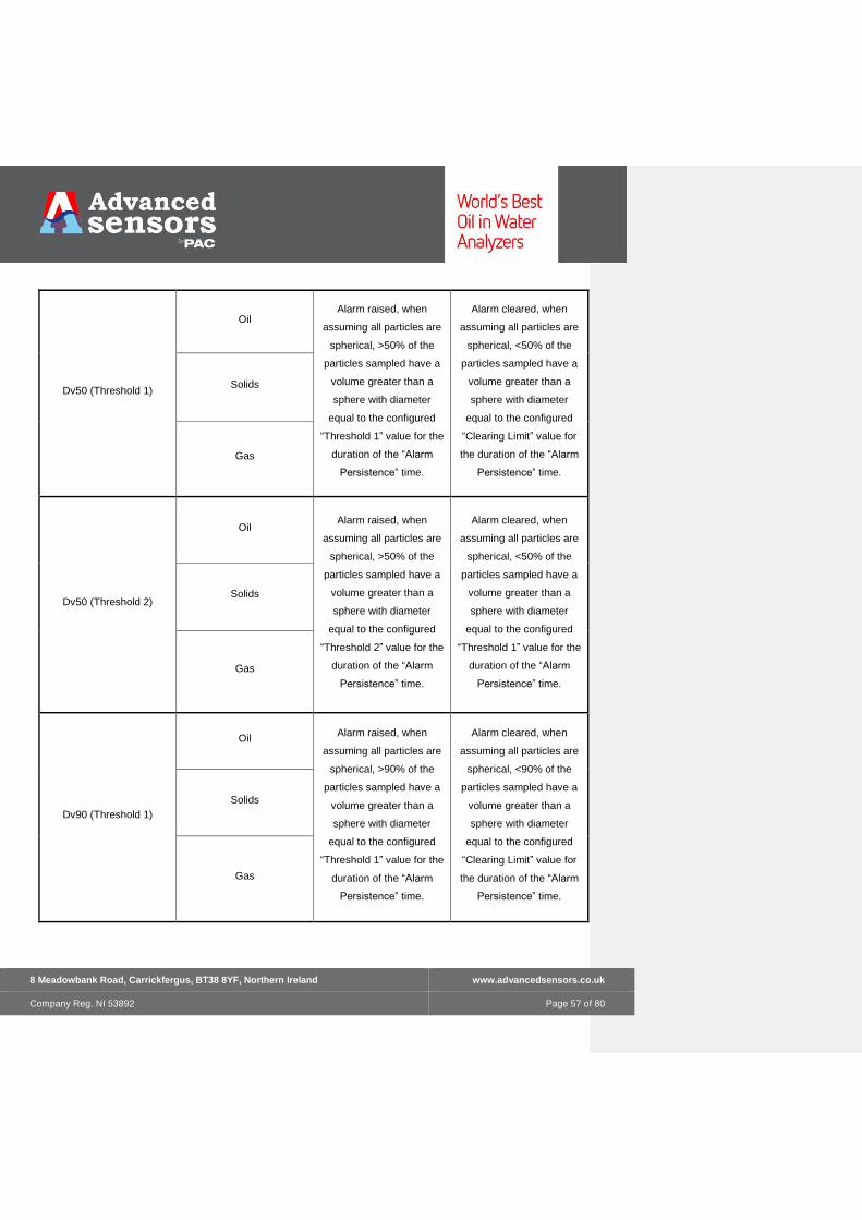
Alarm Type Particle Type Alarm Raise Criteria Alarm Clear Criteria
Image PPM (Threshold 1)
Oil Alarm raised when the
concentration of the
configured particle type is
above the configured
“Threshold 1” value for the
duration of the “Alarm
Persistence” time.
Alarm cleared when the
image PPM is below the
“Clearing Limit” for the
duration of the “Clearing
Persistence” time.
Solids
Gas
Image PPM (Threshold 2)
Oil Alarm raised when the
concentration of the
configured particle type is
above the configured
“Threshold 2” value for the
duration of the “Alarm
Persistence” time.
Alarm cleared when the
image PPM is below the
“Threshold 1” for the
duration of the “Clearing
Persistence” time.
Solids
Gas
Dv10 (Threshold 1)
Oil
Alarm raised, when
assuming all particles are
spherical, >10% of the
particles sampled have a
volume greater than a
sphere with diameter
equal to the configured
“Threshold 1” value for the
duration of the “Alarm
Persistence” time.
Alarm cleared, when
assuming all particles are
spherical, <10% of the
particles sampled have a
volume greater than a
sphere with diameter
equal to the configured
“Clearing Limit” value for
the duration of the “Alarm
Persistence” time.
Solids
Gas
Dv10 (Threshold 2)
Oil Alarm raised, when
assuming all particles are
spherical, >10% of the
particles sampled have a
volume greater than a
sphere with diameter
equal to the configured
“Threshold 2” value for the
duration of the “Alarm
Persistence” time.
Alarm cleared, when
assuming all particles are
spherical, <10% of the
particles sampled have a
volume greater than a
sphere with diameter
equal to the configured
“Threshold 1” value for the
duration of the “Alarm
Persistence” time.
Solids
Gas
8 Meadowbank Road, Carrickfergus, BT38 8YF, Northern Ireland www.advancedsensors.co.uk
Company Reg. NI 53892 Page 57 of 80
Dv50 (Threshold 1)
Oil Alarm raised, when
assuming all particles are
spherical, >50% of the
particles sampled have a
volume greater than a
sphere with diameter
equal to the configured
“Threshold 1” value for the
duration of the “Alarm
Persistence” time.
Alarm cleared, when
assuming all particles are
spherical, <50% of the
particles sampled have a
volume greater than a
sphere with diameter
equal to the configured
“Clearing Limit” value for
the duration of the “Alarm
Persistence” time.
Solids
Gas
Dv50 (Threshold 2)
Oil Alarm raised, when
assuming all particles are
spherical, >50% of the
particles sampled have a
volume greater than a
sphere with diameter
equal to the configured
“Threshold 2” value for the
duration of the “Alarm
Persistence” time.
Alarm cleared, when
assuming all particles are
spherical, <50% of the
particles sampled have a
volume greater than a
sphere with diameter
equal to the configured
“Threshold 1” value for the
duration of the “Alarm
Persistence” time.
Solids
Gas
Dv90 (Threshold 1)
Oil Alarm raised, when
assuming all particles are
spherical, >90% of the
particles sampled have a
volume greater than a
sphere with diameter
equal to the configured
“Threshold 1” value for the
duration of the “Alarm
Persistence” time.
Alarm cleared, when
assuming all particles are
spherical, <90% of the
particles sampled have a
volume greater than a
sphere with diameter
equal to the configured
“Clearing Limit” value for
the duration of the “Alarm
Persistence” time.
Solids
Gas

8 Meadowbank Road, Carrickfergus, BT38 8YF, Northern Ireland www.advancedsensors.co.uk
Company Reg. NI 53892 Page 58 of 80
Dv90 (Threshold 2)
Oil
Alarm raised, when
assuming all particles are
spherical, >90% of the
particles sampled have a
volume greater than a
sphere with diameter
equal to the configured
“Threshold 2” value for the
duration of the “Alarm
Persistence” time.
Alarm cleared, when
assuming all particles are
spherical, <90% of the
particles sampled have a
volume greater than a
sphere with diameter
equal to the configured
“Clearing Limit” value for
the duration of the “Alarm
Persistence” time.
Solids
Gas
Dn10 (Threshold 1)
Oil Alarm raised when 10% of
the particles sampled have
a diameter above
“Threshold 1” for the
duration of the “Alarm
Persistence” time.
Alarm cleared when 10%
of the particles sampled
have a diameter below the
“Clearing Limit” for the
duration of the “Clearing
Persistence” time.
Solids
Gas
Dn10 (Threshold 2)
Oil Alarm raised when 10% of
the particles sampled have
a diameter above
“Threshold 2” for the
duration of the “Alarm
Persistence” time.
Alarm cleared when 10%
of the particles sampled
have a diameter below the
“Threshold 1” for the
duration of the “Clearing
Persistence” time.
Solids
Gas
Dn50 (Threshold 1)
Oil Alarm raised when 50% of
the particles sampled have
a diameter above
“Threshold 1” for the
duration of the “Alarm
Persistence” time.
Alarm cleared when 50%
of the particles sampled
have a diameter below the
“Clearing Limit” for the
duration of the “Clearing
Persistence” Time.
Solids
Gas
Dn50 (Threshold 2)
Oil Alarm raised when 50% of
the particles sampled have
a diameter above
“Threshold 2” for the
duration of the “Alarm
Persistence” time.
Alarm cleared when 50%
of the particles sampled
have a diameter below the
“Threshold 1” for the
duration of the “Clearing
Persistence” Time.
Solids
Gas
Commented [HJ1]: For all you need to add in threshold 2 alarms
8 Meadowbank Road, Carrickfergus, BT38 8YF, Northern Ireland www.advancedsensors.co.uk
Company Reg. NI 53892 Page 59 of 80
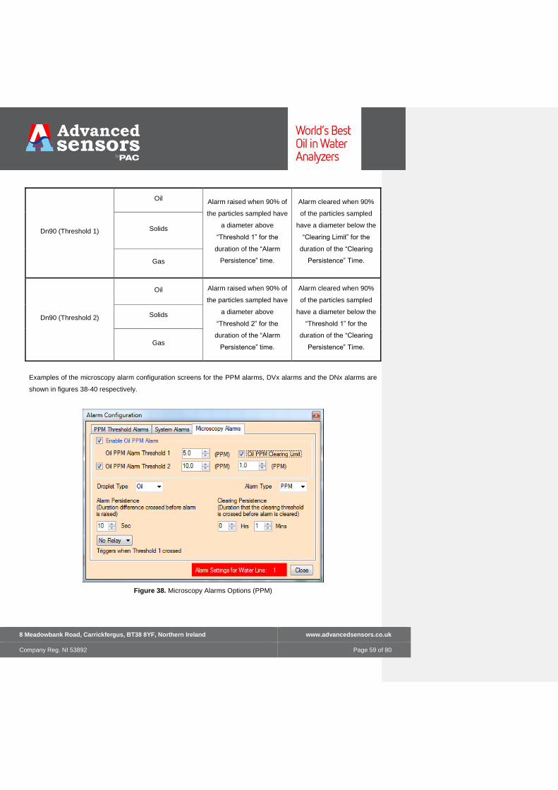
Dn90 (Threshold 1)
Oil Alarm raised when 90% of
the particles sampled have
a diameter above
“Threshold 1” for the
duration of the “Alarm
Persistence” time.
Alarm cleared when 90%
of the particles sampled
have a diameter below the
“Clearing Limit” for the
duration of the “Clearing
Persistence” Time.
Solids
Gas
Dn90 (Threshold 2)
Oil Alarm raised when 90% of
the particles sampled have
a diameter above
“Threshold 2” for the
duration of the “Alarm
Persistence” time.
Alarm cleared when 90%
of the particles sampled
have a diameter below the
“Threshold 1” for the
duration of the “Clearing
Persistence” Time.
Solids
Gas
Examples of the microscopy alarm configuration screens for the PPM alarms, DVx alarms and the DNx alarms are
shown in figures 38-40 respectively.
Figure 38. Microscopy Alarms Options (PPM)

8 Meadowbank Road, Carrickfergus, BT38 8YF, Northern Ireland www.advancedsensors.co.uk
Company Reg. NI 53892 Page 60 of 80
Figure 39. Selecting the Droplet Type
Figure 40. Microscopy Alarms Options (Dn50)

8 Meadowbank Road, Carrickfergus, BT38 8YF, Northern Ireland www.advancedsensors.co.uk
Company Reg. NI 53892 Page 61 of 80
When a microscopy alarm is raised the “Micr. Alarms” button will be highlighted red. Clicking on the button will
show a table of all currently raised alarms. The “Threshold” column shows the trigger value that should be
exceeded in order for the alarm to be raised. The “Clearing Details” column for an active alarm shows the trigger
value below which the alarm will clear. When the alarm is clearing the “Clearing Details” column will show the time
left before the alarm will be cleared. Figure 41 shows an example of an alarm being raised on threshold 1 while the
threshold 2 alarms is clearing.
Figure 41. Microscopy Alarms table showing alarms for the Dv90 alarms for solids
The microscopy alarms can be used to provide external alarms. External alarm capability for each of the
microscopy alarms is enabled via relays. The relay will be triggered if the trigger condition is exceeded for an alarm
that a relay has been assigned to. The relay will be reset when all the alarms it has been assigned to are cleared.
The relay used for each alarm can be chosen from the relay drop down list, as shown below in Figure 42.

8 Meadowbank Road, Carrickfergus, BT38 8YF, Northern Ireland www.advancedsensors.co.uk
Company Reg. NI 53892 Page 62 of 80
Figure 42. Assigned relays can be selected from can be selected from the relays drop down list.
Section 6 – Data Files
Both the analysis and image data are stored for later reference within the OIW EX-M Series units, as with the
standard fluorescence (for OIW EX100M and EX1000M only) and spectral data (for OIW EX1000M only).
To review the Microscopy data, we recommend that you use MiView Software.
6.1 – Location
The Data Logging Handbook provides details for locating the OIWLogs directory in the shared area of the OIW EX-
M Series unit.
The microscopy files are located in a folder named Micro_Logs within the monthly folder either in system
configuration dependent:
8 Meadowbank Road, Carrickfergus, BT38 8YF, Northern Ireland www.advancedsensors.co.uk
Company Reg. NI 53892 Page 63 of 80
C:\Users\Public\Documents\OIWlogs
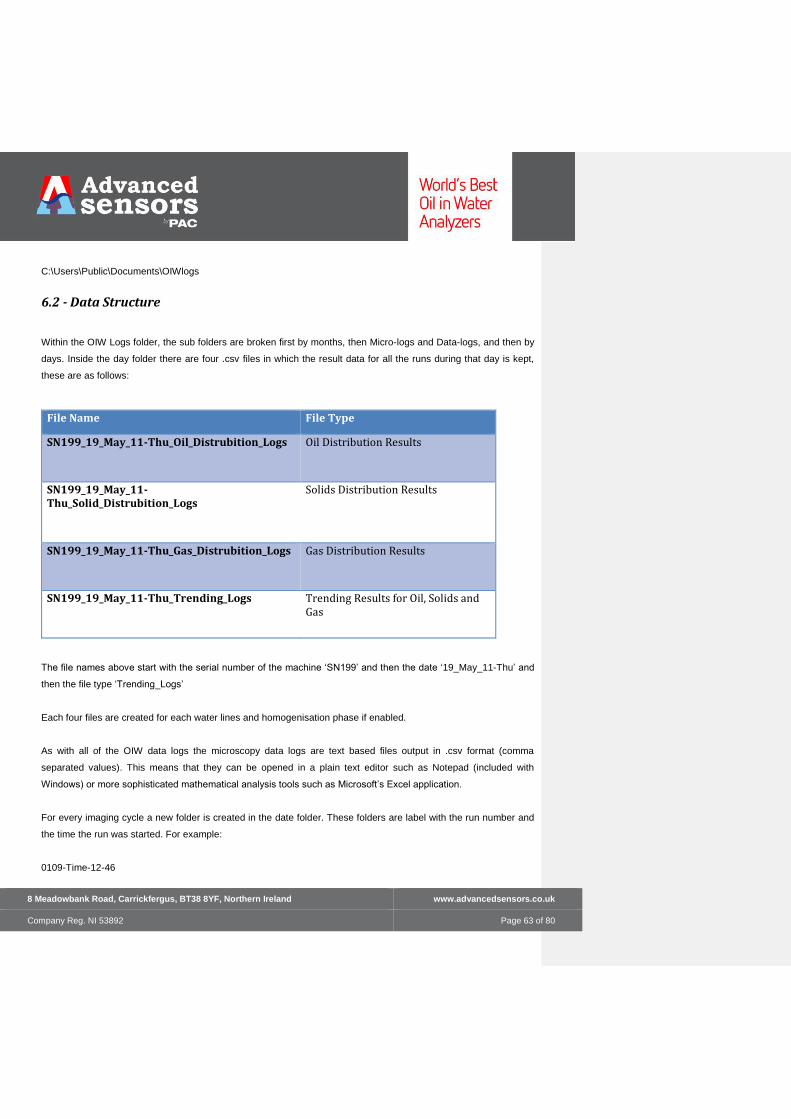
6.2 - Data Structure
Within the OIW Logs folder, the sub folders are broken first by months, then Micro-logs and Data-logs, and then by
days. Inside the day folder there are four .csv files in which the result data for all the runs during that day is kept,
these are as follows:
File Name File Type
SN199_19_May_11-Thu_Oil_Distrubition_Logs
Oil Distribution Results
SN199_19_May_11-Thu_Solid_Distrubition_Logs
Solids Distribution Results
SN199_19_May_11-Thu_Gas_Distrubition_Logs
Gas Distribution Results
SN199_19_May_11-Thu_Trending_Logs
Trending Results for Oil, Solids and Gas
The file names above start with the serial number of the machine ‘SN199’ and then the date ‘19_May_11-Thu’ and
then the file type ‘Trending_Logs’
Each four files are created for each water lines and homogenisation phase if enabled.
As with all of the OIW data logs the microscopy data logs are text based files output in .csv format (comma
separated values). This means that they can be opened in a plain text editor such as Notepad (included with
Windows) or more sophisticated mathematical analysis tools such as Microsoft’s Excel application.
For every imaging cycle a new folder is created in the date folder. These folders are label with the run number and
the time the run was started. For example:
0109-Time-12-46

8 Meadowbank Road, Carrickfergus, BT38 8YF, Northern Ireland www.advancedsensors.co.uk
Company Reg. NI 53892 Page 64 of 80
This would be images from cycle 109 which started at 12:46.
Two images are saved for every image processed. The first image saved is the raw unprocessed image and the
second image is the processed image which contains the results for the image. The processed image is stored with
lower quality as the image itself is only used as a reference. The raw unprocessed image is saved at full quality
allowing these images to be reprocessed at a later stage.
For example the file names of the images are shown below:
Raw Image Filename:- OIWImage0001_19 May 2011_12_28_32
Processed Image Filename:- OIWImageProcessed0001_19 May 2011_12_28_32
The first part of the file name will contain the word ‘OIWImageProcessed’ if it is a processed image and for a raw
image this is ‘OIWImage’. The next four digits is the image number in the run. This is then followed by the date and
time.
8 Meadowbank Road, Carrickfergus, BT38 8YF, Northern Ireland www.advancedsensors.co.uk
Company Reg. NI 53892 Page 65 of 80
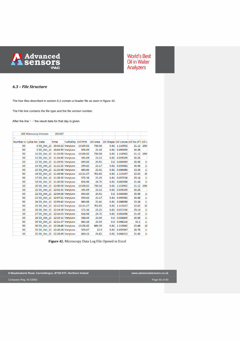
6.3 – File Structure
The four files described in section 6.2 contain a header file as seen in figure 42.
The File line contains the file type and the file version number.
After the line ‘- -‘ the result data for that day is given.
Figure 42. Microscopy Data Log File Opened in Excel

8 Meadowbank Road, Carrickfergus, BT38 8YF, Northern Ireland www.advancedsensors.co.uk
Company Reg. NI 53892 Page 66 of 80
6.4 – File Backup / Removal
To ensure memory management the OIW-EX-M units auto removes older images when hard drive is low on
memory.
It is important to understand that all analysis files will be maintained – and only the image files will be deleted.
Should the images be required longer term then they must be backed up.
8 Meadowbank Road, Carrickfergus, BT38 8YF, Northern Ireland www.advancedsensors.co.uk
Company Reg. NI 53892 Page 67 of 80
7.1 – Measurements This section describes the various measurement values obtained from the OIW Microscopy System.
7.1.1 Shape These values are used to describe the shape of each object and are used to classify the objects found in the
image.
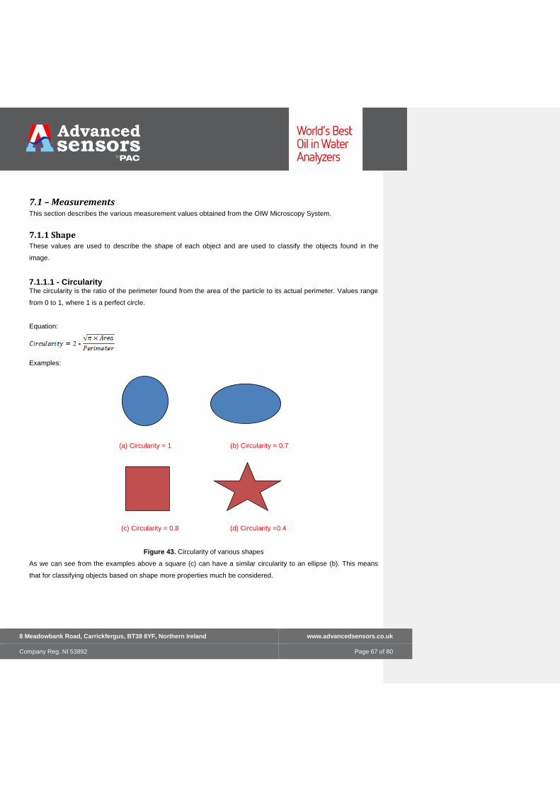
7.1.1.1 - Circularity The circularity is the ratio of the perimeter found from the area of the particle to its actual perimeter. Values range
from 0 to 1, where 1 is a perfect circle.
Equation:
Examples:
(a) Circularity = 1 (b) Circularity = 0.7
(c) Circularity = 0.8 (d) Circularity =0.4
Figure 43. Circularity of various shapes
As we can see from the examples above a square (c) can have a similar circularity to an ellipse (b). This means
that for classifying objects based on shape more properties much be considered.

8 Meadowbank Road, Carrickfergus, BT38 8YF, Northern Ireland www.advancedsensors.co.uk
Company Reg. NI 53892 Page 68 of 80
7.1.1.2 - HS Circularity (High Sensitivity Circularity)
The high sensitivity circularity is more sensitive to the difference in the object’s area to its perimeter than circularity
measurements. Values range from 0 to 1.
Equation:
7.1.1.3 - Convexity
Convexity is an indication of how rough the particle is. The convexity is found from the ratio of the Convex Hull
perimeter divided by actual particle perimeter of the object.
Equation:
The Convex Hull is like placing an elastic band around the object, for example the dotted line around the star object
in figure 44.
Figure 44. Convex Hull around a star shaped object
The lower the convexity the more rough the object is. Convexity ranges from 0 to 1.

8 Meadowbank Road, Carrickfergus, BT38 8YF, Northern Ireland www.advancedsensors.co.uk
Company Reg. NI 53892 Page 69 of 80
7.1.1.4 - Aspect Ratio
The Aspect Ratio is defined as the ratio of the object’s width to its height.
See width and length measurement definitions.
Values range from 0 to 1. A value of 1 would give a perfect circle.
Equation:
7.1.1.5 - Elongation
Elongation is 1 minus the Aspect Ratio
Equation:

8 Meadowbank Road, Carrickfergus, BT38 8YF, Northern Ireland www.advancedsensors.co.uk
Company Reg. NI 53892 Page 70 of 80
7.1.1.6 - Percentage of a Projected Circle
Percentage of the edge of the object that falls within +-10% of a projected circle from the centre of mass of the
object. Figure 45(a) shows a rough circular object where a lot of the object edge falls within the two circular bands,
thus having a high percentage of a projected circle. Whereas the in figure 45(b) the square has very little of its edge
that falls within the two bands, thus having a low percentage of a projected circle.
(a)
(b)
Figure 45. Projected Circle around a rough circular object (a) and square object (b) shape
The shape of the object uses the various shape measurements to calculate how round an object is. The software
uses a specially design Advanced Sensors algorithm to adjust the shape for Oil and Solid particles, making the
classification process unique to this application.

8 Meadowbank Road, Carrickfergus, BT38 8YF, Northern Ireland www.advancedsensors.co.uk
Company Reg. NI 53892 Page 71 of 80
7.1.2 Size
These values are used to describe the size of each object
7.1.2.1 - Volume Distribution
The volume distribution for a set of particles is described by ordering the particles volume and then finding which
particles fall within a certain % of the total volume.
For example, figure 46 shows 3 particles
Particle A, 1µm Diameter
Particle B, 2µm Diameter
Particle C, 3µm Diameter
A B C
Figure 46. Three particles from left to right (a)1µm, (b)2µm and (c)3µm
The volume for each particle is given below and the total volume display from the smallest particle to the largest is
shown in figure 47:
Particle A, 0.52 µm3 Volume
Particle B, 4.2 µm3 Volume
Particle C, 14.1 µm3 Volume
Total Volume is 18.8µm3

8 Meadowbank Road, Carrickfergus, BT38 8YF, Northern Ireland www.advancedsensors.co.uk
Company Reg. NI 53892 Page 72 of 80
Figure 47. Three particles from left to right (a)1µm, (b)2µm and (c)3µm order in terms of volume
10% of the total volume Dv10 of the particles is 1.88µm3 This falls within particle B volume
50% of the total volume Dv50 of the particles is 9.4µm3 This falls within particle C volume
90% of the total volume Dv90 of the particles is 16.92µm3 This falls within particle C volume
Therefore:
Dv10 is 2µm
Dv50 is 3µm
Dv90 is 3µm

8 Meadowbank Road, Carrickfergus, BT38 8YF, Northern Ireland www.advancedsensors.co.uk
Company Reg. NI 53892 Page 73 of 80
7.1.2.2 - Number Distribution
Dn is the distribution of the diameter for the complete volume (objects) that have been sampled. Figure 48 show a
distribution curve.
Figure 48. Distribution Curve
If we order all the objects diameters from the lowest to the highest then:
Dn10 is the diameter 10% of the objects exist
Dn50 is the diameter 50% of the objects exist
Dn90 is the diameter 90% of the objects exist
Dn10 Dn50 Dn90

8 Meadowbank Road, Carrickfergus, BT38 8YF, Northern Ireland www.advancedsensors.co.uk
Company Reg. NI 53892 Page 74 of 80
7.1.2.3 - Diameter/Diameter EQPC
The Diameter EQPC is the diameter of a circle with the equivalent area of the object that is measured, as shown in
figure 49. The Diameter EQPC is used for standard diameter measurements on the analyser including the Dv10,
Dv50 and Dv90.
Area = 65µm Area=65µm
Figure 49. Calculating Diameter based on the area of an object
Equation:
= Diameter

8 Meadowbank Road, Carrickfergus, BT38 8YF, Northern Ireland www.advancedsensors.co.uk
Company Reg. NI 53892 Page 75 of 80
7.1.2.4 - Diameter PED This is the diameter of a circle that has the same perimeter as the object measured
Equation:
7.1.2.5 – Feret Diameter
The Feret Diameter is defined as the maximum distance between any two points in the object, as shown in figure
50.
Figure 50. Feret Diameter of an object
Feret Diameter
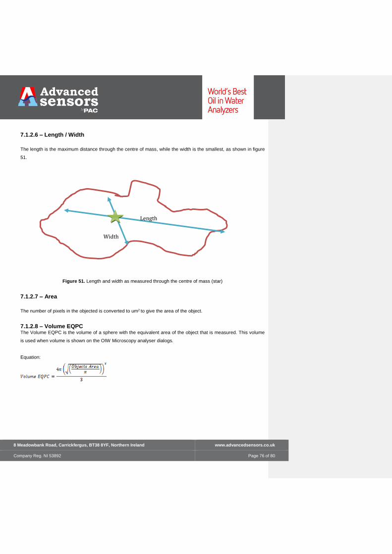
8 Meadowbank Road, Carrickfergus, BT38 8YF, Northern Ireland www.advancedsensors.co.uk
Company Reg. NI 53892 Page 76 of 80
7.1.2.6 – Length / Width
The length is the maximum distance through the centre of mass, while the width is the smallest, as shown in figure
51.
Figure 51. Length and width as measured through the centre of mass (star)
7.1.2.7 – Area
The number of pixels in the objected is converted to um2 to give the area of the object.
7.1.2.8 – Volume EQPC The Volume EQPC is the volume of a sphere with the equivalent area of the object that is measured. This volume
is used when volume is shown on the OIW Microscopy analyser dialogs.
Equation:
Width
Length

8 Meadowbank Road, Carrickfergus, BT38 8YF, Northern Ireland www.advancedsensors.co.uk
Company Reg. NI 53892 Page 77 of 80
7.1.2.9 – Volume PED
This is the volume of a circle that has the same perimeter as the object measured
Equation:
7.1.2.10 – Perimeter
The Perimeter is the distance around the object.
7.1.3 -Concentration
Image PPM
The image PPM is measured for Oil, Solids and Gas objects. The values are found in a three step process:
1. The total area of the objects in the image divided by the area of the image
2. Adjust this value based on the calibration curve for the system
3. Adjust the value for the gain for Oil, Solids and Gas, to get the final PPM
Concentration
The concentration is simply the % of Oil, Solids or Gas measured.
Number of Objects
The number of particles is the number of Oil, Solids or Gas objects found.

8 Meadowbank Road, Carrickfergus, BT38 8YF, Northern Ireland www.advancedsensors.co.uk
Company Reg. NI 53892 Page 78 of 80
7.2 – Configuration Parameters
This section describes the various parameters that are found the in Microscopy Configuration of the OIW
Microscopy Software
Imaging Mode
The system can sample during imaging in three modes. The recommend mode is to image in flow.
1. Static Imaging
The sample chamber is closed and the sample remains static during imaging.
Advantages
• Imaging will not be affected by high flow in this mode.
• Average value of the static sample rather than measuring different points in the flow.
Disadvantages
• If there are high levels of gas in the system, the sudden change in pressure from closing the chamber may
cause gas to be released. This can affect the quality of the images.
• Oil and Solid particles may settle in the sampling chamber over the image period
2. Flow Imaging
Imaging cycle is measured with flow through the chamber. Meaning that for 50 images with 1 second between each
image the result will be the average of 50 seconds of flow for the image cycle.
Advantages
• Not affected by gas.
• No Oil or Solid settling
Disadvantages
• If the flow is too high objects will become distorted. Please contact Advanced Sensors for the maximum
flow rate of your system.

8 Meadowbank Road, Carrickfergus, BT38 8YF, Northern Ireland www.advancedsensors.co.uk
Company Reg. NI 53892 Page 79 of 80
3. High Gas Content
This Mode operates in flow with cleaning between each image the minimum time between each image can only be
3 seconds. Useful if there is a lot of gas sticking to optical window on the analyser.

8 Meadowbank Road, Carrickfergus, BT38 8YF, Northern Ireland www.advancedsensors.co.uk
Company Reg. NI 53892 Page 80 of 80
8 – Appendix
8.1 - OIW-EX Contact Details
Customer Liaison
Sales & Marketing
Tel.+44(0)28 93 35 64 67
E-Mail: [email protected]
Advanced Sensors Headquarters
Advanced Sensors Ltd
8 Meadowbank Road
Carrickfergus
BT38 8YF
UK
Tel: +44 (0)28 93 32 89 22
Fax: +44 (0)28 93 32 86 69
Web: www.advancedsensors.co.uk