Instructions for use

Title Ozone variations over the northern subtropical region revealed by ozonesonde observations in Hanoi

Author(s) Ogino, S.-Y.; Fujiwara, M.; Shiotani, M.; Hasebe, F.; Matsumoto, J.; T. Hoang, Thuy Ha; T. Nguyen, Tan Thanh

Citation Journal of Geophysical Research: Atmospheres, 118(8), 3245-3257https://doi.org/10.1002/jgrd.50348

Issue Date 2013-04-27

Doc URL http://hdl.handle.net/2115/64747

Rights Copyright 2013 American Geophysical Union.

Type article

File Information Ogino_et_al-2013-Journal_of_Geophysical_Research__Atmospheres.pdf

Hokkaido University Collection of Scholarly and Academic Papers : HUSCAP

JOURNAL OF GEOPHYSICAL RESEARCH: ATMOSPHERES, VOL. 118, 3245–3257, doi:10.1002/jgrd.50348, 2013

Ozone variations over the northern subtropical region revealedby ozonesonde observations in HanoiS.-Y. Ogino,1,2 M. Fujiwara,3 M. Shiotani,4 F. Hasebe,3 J. Matsumoto,1,5

Thuy Ha T. Hoang,6 and Tan Thanh T. Nguyen6

Received 4 December 2012; revised 15 March 2013; accepted 19 March 2013; published 30 April 2013.

[1] Seasonal and subseasonal variations in the ozone mixing ratio (OMR) areinvestigated by using continuous 7 year ozonesonde data from Hanoi (21ıN, 106ıE),Vietnam. The mean seasonal variations for the 7 years show large amplitude at the uppertroposphere and lower stratosphere (UTLS) region (10–18 km) and at the lowertroposphere (around 3 km) with standard deviations normalized by the annual mean valueof about 30% for both regions. In the UTLS region, the seasonal variation in the OMRshows a minimum in winter and a maximum in spring to summer. The variation seems tobe caused by the seasonal change in horizontal transport. Low OMR air masses aretransported from the equatorial troposphere in winter by the anticyclonic flow associatedwith the equatorial convections, and high OMR air masses are transported from themidlatitude stratosphere in summer possibly due to Rossby wave breakings in the UTregion and anticyclonic circulation associated with the Tibetan High in the LS region. Inthe lower troposphere, a spring maximum is found at 3 km height. Biomass burning andtropopause foldings are suggested as possible causes of this maximum. Subseasonalvariations in the OMR show large amplitude in the UTLS region (at around 15 km) and inthe boundary layer (below 1 km) with the standard deviations normalized by the annualmean larger than 40%. The OMR variations in the winter UTLS region have a negativecorrelation with the meridional wind. This relation indicates that the low OMRs observedat Hanoi has been transported from the equatorial region.Citation: Ogino, S.-Y., M. Fujiwara, M. Shiotani, F. Hasebe, J. Matsumoto, T. H. T. Hoang, and T. T. T. Nguyen (2013), Ozonevariations over the northern subtropical region revealed by ozonesonde observations in Hanoi, J. Geophys. Res. Atmos., 118,3245–3257, doi:10.1002/jgrd.50348.

1. Introduction[2] Atmospheric ozone is a gas that has activity in both

infrared and ultraviolet-visible regions. In the stratosphere,heating due to ultraviolet absorption by the ozone has anessential role in determining the basic atmospheric struc-ture. In the troposphere, ozone controls the air quality by

1Research Institute for Global Change (RIGC), Japan Agency forMarine-Earth Science and Technology (JAMSTEC), Yokosuka, Japan.

2Graduate School of Science, Kobe University, Kobe, Japan.3Faculty of Environmental Earth Science, Hokkaido University,

Sapporo, Japan.4Research Institute for Sustainable Humanosphere, Kyoto University,

Uji, Kyoto, Japan.5Department of Geography, Tokyo Metropolitan University, Hachioji,

Japan.6Aero-Meteorological Observatory, National Hydrometeorological

Service, Ministry of Natural Resources and Environment, Hanoi, S. R.Vietnam.

Corresponding author: S-.Y. Ogino, Research Institute for GlobalChange (RIGC), Japan Agency for Marine-Earth Science and Technology(JAMSTEC), 2-15, Natsushima-cho, Yokosuka 237-0061, Japan.(ogino-sy@jamstec.go.jp)

©2013. American Geophysical Union. All Rights Reserved.2169-897X/13/10.1002/jgrd.50348

producing OH radical and works as a greenhouse gas [e.g.,Brasseur et al., 2003]. Recently, it was shown that the tropo-spheric ozone is increasing (positive radiative forcing) andcontributes to the global warming [Solomon et al., 2007].However, the observations show that the ozone variation hasstrong dependence on location. In recent decades, increasingozone mixing ratios were observed in high latitudes [e.g.,Tarasick et al., 2005], whereas a decrease was observedover Europe and North America [Logan et al., 2012]. In thestratosphere, it is reported that the ozone amount had a nega-tive trend until the 1990s and is slightly increasing in recentyears [WMO, 2011]. The stratospheric ozone decrease givesboth positive radiative effect due to an increase in solar radi-ation reaching the troposphere and negative one due to adecrease in thermal infrared emission, and the consequentradiative balance is sensitive to the vertical distribution ofozone depletion [Shine and de Forster, 1999]. It is impor-tant to describe the three-dimensional distribution and itstemporal variation of ozone on a global basis in order tounderstand the atmospheric variability and climate change[WMO, 2011].

[3] Satellite observations of ozone have provided abun-dant information, especially about the global distributionof column ozone [e.g., Stolarski and Frith, 2006]. Vertical

3245

OGINO ET AL.: OZONE VARIATION IN HANOI

profiles are observed with the nadia [e.g., Hoogen et al.,1999; Kroon et al., 2011] and limb [e.g., Shiotani andHasebe, 1994; Mieruch et al., 2012] measurement tech-niques which have depicted the three-dimensional ozonedistributions and their variabilities mainly in the middleatmosphere. Although tropospheric ozone profiles are nowavailable by nadir sounding [e.g., Worden et al., 2007], theystill have limitations in the vertical resolution and cover-age. Therefore, balloon-borne ozonesondes remain a neces-sary tool for ozone observation. These ozonesondes haveadvantages in vertical resolution and wide vertical coveragethrough the troposphere and the lower stratosphere (surfaceto �30 km), even though an individual ozonesonde obser-vation does not provide information about the horizontalvariation.

[4] Ozonesonde observations operationally conducted bythe meteorological agencies have a long time and globalcoverage. Most of the operational ozonesonde data arearchived at World Ozone and Ultraviolet Radiation DataCentre (WOUDC) (http://www.woudc.org/). Since the oper-ational ozonesonde stations tend to be located over thenorthern midlatitudes, the Southern Hemisphere AdditionalOzonesondes (SHADOZ) recently established equatorialand southern hemispheric ozonesonde stations [Thompsonet al., 2003a, 2003b, 2007, 2012]. However, there was noozonesonde station before September 2004 that providedcontinuous data over the Indochina Peninsula, which islocated at the southeastern edge of the Eurasian Continent.

[5] Since September 2004, we have conducted once ortwice monthly regular ozonesonde observations in Hanoi(21.02ıN, 105.80ıE) at the base of the Indochina Penin-sula. In addition, we have conducted campaign observationswith ozonesondes and two types of water vapor sondes,Snow White [Fujiwara et al., 2003a] and Cryogenic Frostpoint Hygrometer (CFH) [Vömel et al., 2007], seven timesduring every northern winter from 2004/2005 to 2010/2011[e.g., Fujiwara et al., 2010]. In each campaign observation,ozone and water vapor sondes were launched at intervalsof a few days during a 2–4 week period. Such continu-ous ozonesonde observation in this latitude region is rareon a global basis except for the operational observation atHong Kong (22.31ıN, 114.17ıE) near Hanoi since 2000,where the obtained data are archived at the WOUDC. In thispaper, the data at Hong Kong are also used as a reference.Hanoi has been one of the SHADOZ stations since 2010[Thompson et al., 2012].

[6] Hanoi is located near the boundary between the trop-ical troposphere and extratropical stratosphere in the uppertroposphere and lower stratosphere (UTLS) region, which isone of the important regions for the stratosphere-troposphereexchange (STE) [Holton et al., 1995]. Hanoi is also locatedat the southeastern edge of the Asian monsoon circulation.The Asian monsoon is one of the most important circu-lations for the mass and energy exchanges between thetropics and the extratropics in the UTLS region [Dunkerton,1995]. In the meaning mentioned above, the physical andchemical observations at Hanoi are expected to provide valu-able information on the STE and the tropical-extratropicalexchange. The purpose of this paper is to describe the basicvariations in ozone and related meteorological parametersobtained at Hanoi, the newly established ozonesonde station.From the viewpoint of zonal mean atmospheric structure,

it is expected that the seasonal variation in ozone in thesubtropical UTLS region shows larger (smaller) values inwinter (summer) because the boundary between the midlat-itude LS and the tropical UT moves southward (northward)in winter (summer) and the air mass with high (low) ozoneconcentration in the midlatitude LS (the tropical UT) tendsto be observed. However, it will be shown that the seasonalozone variation at Hanoi is opposite to the one expected fromthe zonal mean viewpoint and is strongly affected by thezonally asymmetric atmospheric structure due to the Asianmonsoon.

[7] In this paper, we describe the seasonal and subseasonalvariations in the ozone mixing ratio (OMR) revealed by theozonesonde observations at Hanoi. In section 2, we describethe details of ozonesonde observations conducted at Hanoi,the other data used for comparison, and the analysis method.The characteristics of seasonal variations and subseasonalvariations in ozone are shown in section 3. The source ofthe variations is discussed by comparing with the meteoro-logical fields and the global ozone distributions. Section 4summarizes the results of the description and the discussion.

2. Observation and Data2.1. Ozonesonde Observation at Hanoi

[8] We started regular ozonesonde observations inSeptember 2004 at the Aero-Meteorological Observatory inHanoi (21.02ıN, 105.80ıE; WMO station number: 48820),Vietnam. We have conducted once-monthly ozonesondeobservations since then. The launch frequency was increasedto twice monthly during the period from February 2006 toOctober 2010.

[9] Seven intensive campaign observations with ozoneand water vapor sondes have been conducted in every north-ern winter (December 2004/January 2005, January 2006,January 2007, January 2008, January 2009, January 2010,and January 2011) under the Soundings of Ozone and Waterin the Equatorial Region (SOWER) project [e.g., Fujiwaraet al., 2010]. During each campaign period (2–4 weeks),we launched ozone and water vapor sondes every few days.The number of intensive ozonesonde launches for each cam-paign is as follows: 8 in the first campaign (December 2004to January 2005), 16 in the second (January 2006), 6 in thethird (January 2007), 5 in the fourth (January 2008), 4 inthe fifth (January 2009), 5 in the sixth (January 2010), and3 in the seventh (January 2011). We use these campaign datato describe the subseasonal and day-to-day variabilities inozone during the wintertime.

[10] The monthly observations were conducted by usinga set of an ozonesonde and a radiosonde to obtain theozone concentration, pressure, temperature, and humiditydata from the surface up to about 30 km. Three types ofozonesonde-radiosonde combinations were used. Dependingon the combinations, different types of sensor solutions wereused. During the period from September 2004 to April 2009,a combination of an Ensci 1Z ECC ozonesonde and a VaisalaRS80 radiosonde without a wind finding module wereused with a 2%-KI unbuffered solution (combination 1).A Science Pump Corporation ECC-6A ozonesonde and aVaisala RS92-SGP radiosonde with a 1%-KI buffered solu-tion (combination 2) were used during the period from May2009 to June 2010. An Ensci Model-Z ECC ozonesonde and

3246

OGINO ET AL.: OZONE VARIATION IN HANOI

Figure 1. (left) Mean seasonal variation of OMR obtained by calculating monthly mean values at eachheight and at each month from September 2004 to November 2011. (center) Same as the left panels butshowing the OMR anomalies from the annual mean at each height. (right) Vertical profiles of annualmean OMR (thick dashed line), standard deviation of OMR mean seasonal variation (thin solid line),and standard deviation normalized by the annual mean OMR at each height (thick solid line). Plus marksin left and center panels indicate cold point tropopauses determined by the long-term monthly meantemperature profiles. The upper panels show the height range of 0–30 km, while the lower panels focuson the variations in the UTLS and the tropospheric regions from 0 to 20 km.

a Vaisala RS92-SGP radiosonde with a 0.5%-KI bufferedsolution (combination 3) have been used since July 2010.The wind data have been available since May 2009 for theobservations launched with the RS92-SGP radiosonde.

[11] In laboratory intercomparisons, differences in ozonevalues measured by ECC ozonesondes with different instru-ment and solution types were shown by Smit et al. [2007].According to their result, combinations 1, 2, and 3 used atHanoi have biases relative to the reference measurementby the UV-photometer of at most –5%, +5%, and +5%,respectively. This means that the comparison between theozonesonde data before and after the switch from combina-tion 1 to combination 2 in May 2009 may have a relativebias of at most 10%. However, the present study does notcontain such a comparison. In section 3.1, we investigatethe 7 year mean seasonal variations. The biases do not affectthe qualitative investigation of the mean seasonal variations,because the usage of instrument-solution combinations doesnot have any seasonal dependence. It is also noted that,since the data taken by the three types of combinationsare mixed when we estimate the monthly mean values, thebiases tend to be canceled out. The exception is the data ofthe winter campaigns in every January. Only combination1, an Ensci 1Z ECC ozonesonde and a 2%-KI unbufferedsolution, has been used for the campaign observations.Therefore, the monthly mean data in January may have anegative bias relative to other months. However, this bias isconsidered to be negligible in this paper, because we willexamine the seasonal variability larger than 20–30%. This

point will be mentioned again in section 3.1. In section 3.2,we investigate the subseasonal and day-to-day variabili-ties by using non-averaged data, in which the precision ofthe measurements with the fixed instrument and solutionshould be taken into account. According to the result bySmit et al. [2007], the precision for each sensor type andsolution is less than 5%. That is much smaller than thevariabilities discussed in section 3.2. Note that recently itis planned to homogenize the ozonesonde data sets fromdifferent types of solutions and sensors in an activity,“Ozone Sonde Data Quality Assessment (O3S-DQA),” asa part of SPARC-IGACO-IOC Initiative on “Past Changesin the Vertical Distribution of Ozone” (Smit et al., 2012,Guide Lines for Homogenization of Ozone Sonde Data,http:// www - das.uwyo.edu/�deshler/ NDACC _ O3Sondes/O3s_DQA/O3S-DQA-Guidelines%20Homogenization-V2-19 November2012.doc).

[12] In this paper, we discuss the time variations of theOMR at various time scales at various height regions fromthe surface to the stratosphere. Because the OMR variesrapidly with height, it is reasonable to evaluate the ampli-tude of variation by quantities relative to the mean. Here,the amplitude is evaluated by the “relative standard devia-tion” (RSD). A RSD is defined as a standard deviation (SD)divided by a mean; the RSD is also called the “coefficient ofvariation” in general.

[13] In this paper, we also use the weekly ozonesonde dataobtained at Hong Kong (22.31ıN, 114.17ıE) during 2000–2011 provided by WOUDC. The data were processed by thesame methods as the Hanoi data and used as a reference.

3247

OGINO ET AL.: OZONE VARIATION IN HANOI

Figure 2. The same as Figure 1 except for the results obtained from the ozonesonde data at Hong Kongfrom 2000 to 2010.

2.2. Global Meteorological and Ozone Data[14] To interpret the ozone variations observed at Hanoi,

we also analyzed the global reanalysis and satellite ozonedata. We used the National Centers for Environmental Pre-diction (NCEP) Reanalysis-II data [Kanamitsu et al., 2002]with temporal interval of 6 h, horizontal resolution of2.5�2.5°, and pressure levels of 1000, 925, 850, 700, 600,500, 400, 300, 250, 200, 150, 100, 70, 50, 30, 20, and 10 hPaduring 2004–2010 for analyzing the meteorological fieldsrelated to the ozone variations observed at Hanoi and tocalculate isentropic backward trajectories.

[15] We also used the ozone profiles retrieved by theAura/Microwave Limb Sounder (MLS) retrieval schemeversion 2.2 Level 2 [Livesey et al., 2006; Jiang et al., 2007]to investigate the horizontal distributions of ozone. TheAura/MLS data were chosen because these resolve the ver-tical distribution, and the data period (from August 2004to the present) just covers the ozonesonde observations atHanoi. We exclude from our analysis the data below 215 hPathat is the lowest level of Aura/MLS ozone measurements.We removed the MLS data with erroneous values from ouranalysis in accordance with the recommendations in thedata description document by the Jet Propulsion Labora-tory [Livesey et al., 2007]. The pressure levels used are215.443 (the lowest level of the Aura/MLS ozone mea-surements), 146.780, 100.000, 68.1292, 46.4159, 31.6228,21.5443, 14.6780, 10.0000, 6.81292, and 4.64159 hPa (veryfew ozonesonde data are available above this level). The cli-matological monthly means for the 8 years were obtainedfrom the monthly mean data gridded on to 5ı � 5ı bins.

[16] In addition, we used the monthly mean outgo-ing long-wave radiation (OLR) provided by the NationalOceanic and Atmospheric Administration (NOAA)[Liebmann and Smith, 1996] with a horizontal resolution of

2.5° longitude � 2.5° latitude from 2004 to 2010 to comparethe ozone variations with the convective activities.

3. Results and Discussion3.1. Seasonal Variations

[17] Figure 1 shows the mean seasonal variations of OMRat Hanoi (left panels). The long-term monthly mean val-ues since September 2004 are used for this plot. The OMRanomaly from the annual mean is also shown in the cen-ter panels. The means, the SDs, and the RSDs (the SDsnormalized by the annual mean) are plotted in the right pan-els of Figure 1. The similar plots obtained by the data atHong Kong are shown in Figure 2. The results showed quitesimilar seasonal variations at both stations, suggesting thatthe data are reliable and the obtained variations are robust.The characteristics of the mean seasonal variation seen atboth stations are described below.

[18] In the lower and middle stratosphere (above about20 km height, shown in the upper panels of Figure 1), aclear seasonal variation is found with larger values in springand summer and with smaller values in winter. The meanvalue and the SD rapidly increase with height, while theRSD ranges by 5%–10% through this height range. Sincethe normal SD tends to increase for the variable with largemean value, the RSD is more appropriate for the evalu-ation of variables of which mean value rapidly changes.The seasonal variation with the spring-summer maximumis consistent with the well-known features of seasonal vari-ation in the ozone shown by Shiotani and Hasebe [1994]using satellite ozone data. This reflects the seasonality ofboth the Brewer-Dobson circulation and the photochem-ical production. This aspect of seasonality will not bediscussed further.

3248

OGINO ET AL.: OZONE VARIATION IN HANOI

Figure 3. Upper panels show 5 day backward trajectories starting at every 06:00 UT (13:00 LT inVietnam) the Aura/MLS OMR (color shades) and the NCEP Reanalysis pressure (broken contours) in(left) January, (center) May, and (right) July at 400 K surface (at about 18 km over Hanoi). Lower panelsshow climatological monthly mean geopotential height (color shade), horizontal wind (arrow), and OLR(contour and gray shade) in (left) January, (center) May, and (right) July at 100 hPa (about 400 K nearHanoi). Contour levels for OLR are 180, 200, 220, and 240 W/m2. The areas below 180 and 200 W/m2

are shaded by dark and light gray colors, respectively. Note that OLR contours in the area north of 30ıNare not displayed, because they are possibly contaminated by the cold land surface.

[19] A clear seasonal cycle with a winter minimum isalso found in the upper troposphere and lower stratosphere(UTLS) region (10–20 km shown in the lower panels ofFigure 1) with the RSD of 20–30%. In more detail, the RSDhas double peaks in height at about 14 km and about 18 km.The seasonal variability appears to be different above andbelow the cold point tropopause (indicated by the plus marksin Figure 1) at around 17 km height. Below the tropopauselevel (upper troposphere near 14 km), the OMR peaks in

late spring (May), while above it (lower stratosphere near18 km) the OMR peaks in summer (July to August). Itis possible that the processes resulting in these variationsare different. This point is discussed below in terms of theair mass transport. It should be noted that the winter mini-mum in January should be considered carefully because thedata in January may have a negative bias as mentioned insection 2. It is confirmed that the data at the Hong Kongstation in Figure 2 show the similar minimum in January.

Figure 4. The same as Figure 3 but (upper) at 356 K surface (at about 14 km over Hanoi) and (lower)at 150 hPa (about 356 K near Hanoi).

3249

OGINO ET AL.: OZONE VARIATION IN HANOI

Figure 5. Latitude-pressure section of climatological mean Aura/MLS OMR in May along 105ıE.Black contours show the NCEP Reanalysis isentropes, and gray contours show the NCEP Reanalysiszonal wind.

Therefore, it is said that the minimum in January may notbe caused only by the expected negative bias but reflectsthe nature.

[20] The upper panels of Figure 3 show 5 day backwardtrajectories starting from Hanoi at every 06:00 UT (13:00 LTin Vietnam) in winter (January), late spring (May), andsummer (July) for all years at the 400 K isentropic surface(about 18 km height over Hanoi) and at the 356 K surface(about 14 km height over Hanoi). The backward trajectorieswere calculated every 30 min on isentropic surfaces by usingthe linearly interpolated NCEP reanalysis data and by thesecond-order Runge-Kutta method for time integration, asdone previously by Fujiwara et al. [2003b] and Hasebe et al.[2007]. The monthly mean background OMRs obtained byAura/MLS during 2004–2010 are also plotted in the upperpanels of Figure 3. Corresponding meteorological fields, thegeopotential height, horizontal winds, and OLR are shownin the lower panels of Figure 3, and the same plots for uppertroposphere (around 14 km height near Hanoi) are shown inFigure 4. Note that the white color region over and aroundthe Tibetan Plateau (30ıE–100ıE, 20ıN–50ıN) in the panelfor July at 356 K indicates that the Aura/MLS OMR dataare not available because the level is below the lower limit(215 hPa) of the Aura/MLS ozone observation [Liveseyet al., 2007], which is due to the Tibetan High developmentover the region as seen in the lower right panel of Figure 4.In the following, the overall features of trajectories in eachmonth are compared with the climatological mean of theAura/MLS OMR and the meteorological fields.

[21] In winter, air masses are transported from the equa-torial and subtropical upper troposphere over the MaritimeContinent, the Indian Ocean, South Asia, and West Africawhere the mean OMRs are smaller than those in the

midlatitude and high-latitude regions. This feature is com-monly seen through the UTLS region in winter. The anti-cyclonic circulation formed over the northern part of thewestern Pacific in winter (lower left panels of Figures 3and 4) is considered to be a Rossby response to the convec-tive heating over the Maritime Continent and the equatorialwestern Pacific region [Highwood and Hoskins, 1998;Hatsushika and Yamazaki, 2003]. It is assumed that this typeof horizontal transport is the cause of the OMR minimum inwinter UTLS region over Hanoi.

[22] In late spring (May), convective center moves north-westward, and the associated monsoon high and anticycloniccirculation begin to develop in the UTLS region over andaround the Bay of Bengal as seen in the lower middlepanels of Figures 3 and 4. As seen in Figure 1, the uppertropospheric OMR over Hanoi increases in May at theheight range from 10 to 16 km. This increase is consis-tent with the cross-tropopause, isentropic air mass transportfrom the midlatitude stratosphere possibly due to the Rossbywave breaking, which is known to occur frequently inlate spring at around the 350 K surface [e.g., Appenzelleet al., 1996; Seo and Bowman, 2001]. We emphasize thatthe location of Hanoi is appropriate for the observationof the cross-tropopause mass exchange in this season. Insummer (July), the region of high ozone concentration atthe 356 K surface moves to the Pacific region, as seen inthe lower right panel of Figure 4, and the OMR aroundHanoi decreases. This move is consistent with the results byPostel and Hitchman [1999], who showed that the Rossbywave breaking occurs most actively in the Pacific region inthe northern summer.

[23] At the 400 K surface, a similar anticyclonic flowseems to transport the midlatitude air to the tropics (lower

3250

OGINO ET AL.: OZONE VARIATION IN HANOI

Figure 6. Time height sections of (left) OMR, (center) OMR anomaly from the mean seasonal variation,and (right) vertical profiles of the RSD (the SD of the OMR anomaly from the mean seasonal variationnormalized by the annual mean of each year) from (top) 2004 to (bottom) 2011.

right panel of Figure 3). However, the OMR distribution(upper right panel of Figure 3) formed by the anticycloniccirculation is somewhat different from that in the uppertroposphere. As seen in the upper center and right panelsof Figure 4, the horizontal OMR distribution in the lowerstratosphere has a coherent tongue-shaped structure extend-ing from the central Pacific to the Indian Ocean with ahorizontal scale of �1000 km or larger. It should also benoted that this tongue-shaped structure is vertically sepa-rated from the upper tropospheric ozone increase, as shownin Figure 5. In Figure 5, a high OMR intrusion is seen fromthe midlatitude stratosphere at a latitude of 20ıN–30ıN nearthe 360K surface, while apart from the intrusion, an OMRincrease is seen near 10ıN at around the 380 K surface,which is due to the tongue-shaped OMR transport from the

midlatitude stratosphere. The lower stratospheric increaseseems to be caused directly by the anticyclonic circulationassociated with the Tibetan High, which is different fromthe upper tropospheric increase possibly due to the Rossbywave breakings. This feature is consistent with the resultsof chemical transport model and the data analyses shownby Konopka et al. [2010]. The anticyclonic circulation inthe lower stratosphere appears in late spring and developsuntil midsummer as a thermodynamical response of Asianmonsoon convective activity [Randel and Park, 2006;Park et al., 2007]. In July–August, a well-developedtongue-shaped structure with high OMR air massesmoves over Hanoi. As a result, the maximum OMR isconsidered to appear at around 18 km height in summerover Hanoi.

3251

OGINO ET AL.: OZONE VARIATION IN HANOI

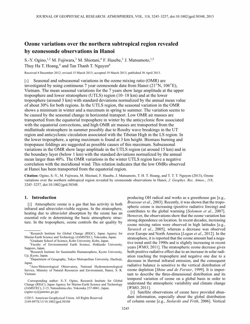
Figure 7. Temporal variations of the OMR averaged at(bottom) 2–4 km, (center) 13–15 km, and (top) 17–19 kmbins in each year from 2004 to 2011. The climatologicalseasonal variation is also plotted with black line.

[24] Hanoi is located at the northwestern edge andat the southeastern edge of the anticyclonic circulationdue to the Rossby response in winter and in sum-mer, respectively. Therefore, it is concluded that the sea-sonal variation in the UTLS ozone observed at Hanoiis caused by the seasonal change in the source of theair mass associated with the large-scale, monsoon-relatedcirculation change, although the detailed behaviors aredifferent between the height ranges above and belowthe tropopause.

[25] In the middle troposphere (5–10 km), the seasonalvariability of OMR is small with the relative standarddeviation of 10%–20% as seen in Figure 1. The weakmaxima are seen in late spring (May), summer (August), andautumn (October).

[26] In the lower troposphere, the OMR has a clear maxi-mum in March to April at about 3 km height. It is known thatsurface ozone enhancement occurs in this season in the Eastand Southeast Asian regions [e.g., Pochanart et al., 2001;Tanimoto et al., 2005]. Pochanart et al. [2001] indicated thatthe spring maximum of the surface ozone over Thailand wascaused by the ozone production due to biomass burning inSoutheast Asia. Indeed, it is clearly seen that the near-surfaceozone increases during the same months. It is possible thatthe ozone increase at about 3 km height is related withthe surface ozone enhancement due to the biomass burn-ing through vertical diffusion or transport. It is knownthat strong temperature inversions frequently develop overthe Indochina Peninsula in spring [Nodzu et al., 2006; Oginoet al., 2010; Nodzu et al., 2011]. Nodzu et al. [2006] showedthat the temperature inversions typically appear at two lev-els, about 1.5 km and about 4 km in March to April overHanoi. It is interesting that the OMR maximum observedwith the ozonesondes appears between the heights of thesedouble inversions. This relationship implies that the dou-ble layered structure of atmospheric stability plays a role indetermining the vertical transport or accumulation processof high OMR air masses over the Indochina Peninsula.

[27] Deep intrusions of the stratospheric air into the tro-posphere associated with tropopause foldings [e.g., Elbernet al., 1997; Stohl et al., 2003] are another candidate forproducing the spring ozone maximum at 3 km. This ozonemaximum also seems to have a source from the upper tropo-spheric ozone increase in May discussed above. The warmair intrusion from the stratosphere due to the tropopausefolding must produce a steep temperature change withinthe troposphere, which is consistent with the coexistence oftemperature inversions and ozone maximum.

[28] The results and discussions above suggest that theconsideration of three-dimensional transport is important forunderstanding the spring increase in ozone at 3 km. Furtherstudies, such as three-dimensional trajectory analysis andnumerical experiments using a chemical transport model, areexpected to clarify the generation mechanism of the ozonemaximum in spring.

[29] An ozone enhancement near the surface in October isalso clearly seen in Figure 1, as also seen in Figure 3 of thepaper by Thompson et al. [2012]. The same feature is foundin the result at Hong Kong (Figure 2). Biomass burning isnot active in October over the southeast Asian region [e.g.,Duncan et al., 2003], which is different from the spring casementioned above. Therefore, we should consider the causeof this enhancement other than the pollution due to biomassburning. Further studies would be expected to clarify it.

3.2. Subseasonal Variations[30] Next, we investigate the subseasonal variations in

OMR observed by the ozonesondes at Hanoi. Figure 6shows the OMR variations for every year from 2004 to2011. The left panels show the OMR measured values. Thecenter panels show the OMR anomalies from the 8 yearmean seasonal variation, i.e., deseasonalized OMR varia-tions. The right panels show vertical profiles of the RSD ofthe deseasonalized OMR variations. Both the data from themonthly and the intensive campaign observations were usedfor these figures. From the left and center panels, we find the

3252

OGINO ET AL.: OZONE VARIATION IN HANOI

Figure 8. Time height sections of (left) OMR and (center) meridional wind, and (right) vertical profilesof statistical values of OMR: (thick dashed line) campaign-mean OMR, (thin solid line) standard devi-ation, and (thick solid line) relative standard deviation for (top) the first (December 2004 and January2005), (middle) the second (January 2006), and (bottom) the third (January 2007) campaign observations.Vertical white lines in the time height sections denote the launch time of the ozonesonde.

subseasonal variations have a significant magnitude in addi-tion to the mean seasonal variability.

[31] These features are more clearly seen from the lineplots at selected heights shown in Figure 7. We can rec-ognize the characteristics of the mean seasonal variationof the OMR with the lower tropospheric (2–4 km) earlyspring (March–April) maximum, the upper tropospheric(13–15 km) late spring (May–June) maximum, and the lowerstratospheric (17–19 km) summer (July–August) maximumin almost all years. In addition to such a clear seasonalcycle, the subseasonal variation of the OMR is also dominantthrough the year.

[32] The RSD for each year is shown in the right panelof Figure 6. It is seen that the RSDs have larger values inthe UTLS region near 15 km height as a common featurefor every year except for years 2010 and 2011. Their val-ues are around 40%, which is comparable to that of themean seasonal variation at the same height region. Note thatthe exception for years 2010 and 2011 is considered partlybecause of the gap in the data. The RSDs in the boundarylayer (below 1 km height) are also large.

[33] The monthly ozonesonde observations at Hanoi havebeen conducted once or twice per month, and their samplinginterval is not constant. Therefore, it is difficult to investigatethe dominant phenomena only from this data set. However,

we have conducted campaign ozonesonde observations atintervals of a few days during every winter. Here, we exam-ine the campaign observation data to investigate the ozonevariations at a time scale of a few to several days.

[34] Examples of OMR variations during the first, second,and third campaigns are shown in Figure 8. The layeredOMR minima with a vertical scale of 2–3 km in the UTLSregion near the 15 km height are clearly seen for all the threecampaign observations. For example, in the first campaign

Figure 9. Vertical profile of mean OMR relative standarddeviation for the results of all campaign observations.

3253

OGINO ET AL.: OZONE VARIATION IN HANOI

Figure 10. Scatter plots of OMR versus meridional wind averaged at height ranges of (left) 14–15 kmand (right) 0–1 km for (top) the first (December 2004 and January 2005), (middle) the second (January2006), and (bottom) the third (January 2007) campaign observations.

period, an OMR minimum appears near the 14 km heightduring 4–8 January. Similar OMR minima are found dur-ing 17–29 January 2006 at around 14 km and during 10–14January 2007 at around 13 km. Vertical profiles of OMRRSDs are shown in the right panels in Figure 8. In this figure,the large variability of ozone in the UTLS is found with theRSD of 40%–60% near the 14 km height. The similar fea-ture (maximum RSD of about 30% in the UTLS region) isfound in the mean RSD profile for all the results from theseven campaigns in every winter (Figure 9). It is also seenthat the near-surface variations have large amplitudes withthe RSD of 40%–70%.

[35] The variation in the UTLS region seems to havea close relation with the background meridional wind asshown in the center panels of Figure 8. This relation isexamined in more detail below, since it supports the resultof the backward trajectory analyses shown in section 3.1that the OMR value observed at Hanoi has a dependencyon the air mass origin. The strong northward wind in theUTLS region coincides with the OMR minima describedabove. The scatter plots show a negative correlation betweenthe OMR and the meridional wind variations averaged over14–15 km height range as shown in the left panels inFigure 10. The correlation coefficient is estimated as approx-imately –0.6 as the mean value of the three campaign data.It is also found that the OMR has a positive correlation

with the zonal wind with the correlation coefficient ofapproximately +0.8 (not shown). These results indicate thatthe eastward-oriented (weak northward and strong east-ward) wind tends to transport low OMR air masses and thenorthward-oriented (strong northward and weak eastward)wind tends to transport high OMR air masses to Hanoi. Inthe boundary layer, a positive correlation between the OMR

Figure 11. Vertical profiles of correlation coefficientbetween the OMR and the meridional wind (left panel) andbetween the OMR and the zonal wind (right panel) at every1 km bin from the surface up to 20 km. The correlation coef-ficient is the averaged value for the results of all campaignobservations.

3254

OGINO ET AL.: OZONE VARIATION IN HANOI

Figure 12. Backward trajectories at 356 K surface starting at the time of campaign ozonesonde launchesfor (left) December 2004 and January 2005, (center) January 2006, and (right) January 2007. Monthlymean Aura/MLS OMR is shaded by color. Lines and shades share the same colors showing the values ofozone mixing ratio.

and the meridional wind is found with a correlation coeffi-cient of approximately 0.4 as the mean value of the threecampaign data.

[36] Figure 11 shows vertical profiles of the correlationcoefficient between the OMR and the meridional wind (leftpanel) and between the OMR and the zonal wind (rightpanel) at every 1 km bin from the surface to 20 km. Thecorrelation coefficient is the average of all results from theseven wintertime campaign observations. It is found thatthe negative (positive) correlation between the OMR andthe meridional (zonal) wind in the UTLS region is a promi-nent feature. The student’s t test for the null correlationbetween OMR and meridional wind in UTLS in January2006, when we conducted 14 soundings that were the largestnumber among the all winter campaigns, showed that thenegative correlation is statistically significant at the 95%level. Based on these facts, we consider that the correlationsbetween OMR and the horizontal winds are the signifi-cant feature in the UTLS region at Hanoi. In the boundarylayer, on the other hand, the positive correlation between theOMR and the meridional wind does not seem to be robust,although the large amplitude and the positive correlation areseen in the first three campaign observations.

[37] In the left panels of Figure 12, backward trajectorieson the 356 K surface starting at Hanoi at the launch time ofthe first, second, and third campaign ozonesonde observa-tions are plotted with colors indicating the observed OMRvalues. These trajectories show that the lower (higher) OMRvalues tend to be traced back to the Maritime Continentsand the western Pacific (to the Indian Ocean and Africanregion). This result is consistent with the negative correla-tion between the OMR and the meridional wind in the UTLSregion over Hanoi and supports the interpretation that theOMR winter minimum in the UTLS is caused by the lowOMR air mass transport from the equatorial region wherethe mean ozone concentration is low.

4. Summary[38] We have conducted continuous monthly ozonesonde

observations and intensive campaign observations withintervals of a few days for every winter at Hanoi (21.02ıN,105.80ıE), Vietnam since September 2004. By using theobtained data, seasonal and subseasonal variations in theozone mixing ratio (OMR) are investigated, and the causes

of the variations are discussed. The relative standarddeviation (RSD), which is defined as the standard deviationnormalized by the mean value, is employed to evaluate theamplitude of variation to eliminate the rapid increase of themean OMR with height.

[39] In the lower and middle stratosphere (above about20 km height), a clear seasonal variation is found with largervalues in spring and summer and with smaller values in win-ter. This result is consistent with the well-known features ofseasonal variation shown in previous studies [Shiotani andHasebe, 1994].

[40] A seasonal cycle with a winter minimum and aspring-summer maximum is also found in the UTLS region(10–20 km) with larger RSD of 20%–30%. A backward tra-jectory analysis shows that the winter minimum is due to thelow OMR air mass transport from the tropical troposphere.This feature is commonly seen through the UTLS regionin winter. In contrast, the variation from spring to summerseems to be different above and below the tropopause levelat around 17 km. Below the tropopause level (upper tropo-sphere near 14 km), the OMR peaks in late spring (May).This peak is consistent with the air mass transport from themidlatitude stratosphere to the troposphere possibly due toRossby wave breakings. Above the tropopause level (lowerstratosphere near 18 km), the OMR peaks in summer (July toAugust). This peak seems to be caused directly by the anti-cyclonic circulation associated with the Tibetan High, whichis different from the upper tropospheric increase. In midsum-mer, the well-developed tongue-shaped structure with highOMR air masses moves over Hanoi. As a result, the maxi-mum OMR is considered to appear at around 18 km heightin summer over Hanoi.

[41] In the lower troposphere, the OMR has a clear maxi-mum in March to April at about 3 km height. The maximumseems to propagate downward from 3 km height to the sur-face ozone maximum in May. The relation with surfaceozone enhancement due to biomass burning is suggested.Tropopause folding is another candidate for producing thespring ozone maximum at 3 km.

[42] Subseasonal variations in the OMR show largeamplitudes in the UTLS region (around 15 km) and in theboundary layer (below 1 km) with the RSD larger than 40%,which is comparable to those of mean seasonal variationof the OMR. It is shown that the OMR variation in theUTLS region during every winter campaign has a negative

3255

OGINO ET AL.: OZONE VARIATION IN HANOI

correlation with the meridional wind. This relationindicates that the low OMR air masses observed at Hanoihave been transported from the equatorial region, whichis confirmed by the backward trajectory analyses. Theseresults support the interpretation that the OMR winter min-imum in the UTLS is caused by the low OMR air masstransport from the equatorial region, where the mean ozoneconcentration is low.

[43] Acknowledgments. The authors thank the staff at the Aero-Meteorological Observatory, Hanoi, National Hydrometeorological Serviceof Vietnam for their help in obtaining the valuable ozonesonde data. Thepresent work was partly supported by Grants-in-Aid for Scientific Research(A) No. 15204043 and (A) No. 18204041, the Ministry of Education, Cul-ture, Sports, Science and Technology, by the Global Environment ResearchFund (A-071), the Ministry of the Environment, and by Kyoto UniversityActive Geosphere Investigations for the 21st Century Centers of Excellence(COE) Program. Some of the ozonesondes were provided by the NationalOceanic and Atmospheric Administration (NOAA) and the National Aero-nautics and Space Administration (NASA). The trajectory model usedin this study was developed at the Earth Observation Research Center(EORC), National Space and Development Agency (NASDA) (now JapanAerospace Exploration Agency, JAXA).

ReferencesAppenzelle, C., J. R. Holton, and K. H. Rosenlof (1996), Seasonal varia-

tion of mass transport across the tropopause, J. Geophys. Res., 101(D10),15,071–15,078.

Brasseur, G. P., R. G. Prinn, and A. A. Pszenny (eds.) (2003), AtmosphericChemistry in a Changing World, 300 pp., Springer-Verlag, Berlin.

Duncan, B. N., R. V. Martin, A. C. Staudt, R. Yevich, and J. A. Logan(2003), Interannual and seasonal variability of biomass burning con-strained by satellite observations, J. Geophys. Res., 108(D2), 4100, doi:10.1029/2002JD002378.

Dunkerton, T. J. (1995), Evidence of meridional motion in the summerlower stratosphere adjacent to monsoon regions, J. Geophys. Res., 100,16,675–16,688.

Elbern, H., J. Kowol, R. Sládkovic, and A. Ebel (1997), Deep stratosphericintrusions: A statistical assessment with model guided analyses, Atmos.Environ., 31(19), 3207–3226, doi:10.1016/S1352-2310(97)00063-0.

Fujiwara, M., M. Shiotani, F. Hasebe, H. Vömel, S. J. Oltmans, P. Ruppert,T. Horinouchi, and T. Tsuda (2003a), Performance of the Meteolabor“Snow White” chilled-mirror hygrometer in the tropical troposphere:Comparisons with the Vaisala RS80 A/H-Humicap sensors, J. Atmos.Oceanic Technol., 20, 1534–1542, doi:10.1175/1520-0426(2003)020.

Fujiwara, M., S.-P. Xie, M. Shiotani, H. Hashizume, F. Hasebe, H.Vömel, S. J. Oltmans, and T. Watanabe (2003b), Upper tropospheric

inversion and easterly jet in the tropics, J. Geophys. Res., 108(D24, 4796),doi:10.1029/2003JD003,928.

Fujiwara, M., et al. (2010), Seasonal to decadal variations of water vaporin the tropical lower stratosphere observed with balloon-borne cryo-genic frost point hygrometers, J. Geophys. Res., 115 (D18304), doi:10.1029/2010JD014179.

Hasebe, F., M. Fujiwara, N. Nishi, M. Shiotani, H. Vömel, S. Oltmans, H.Takashima, S. Saraspriya, N. Komala, and Y. Inai (2007), In situ obser-vations of dehydrated air parcels advected horizontally in the tropicaltropopause layer of the western Pacific, Atmos. Chem. Phys., 7, 803–813,doi:10.5194/acp-7-803-2007.

Hatsushika, H., and K. Yamazaki (2003), Stratospheric drain over Indone-sia and dehydration within the tropical tropopause layer diagnosedby air parcel trajectories, J. Geophys. Res., 180D19, 4610, doi:10.1029/2002JD002986.

Highwood, E. J., and B. J. Hoskins (1998), The tropical tropopause, Q. J.R. Meteorol. Soc., 124, 1579–1604.

Holton, J. R., P. H. Haynes, M. E. McIntyre, A. R. Douglass, R. B. Rood,and L. Pfister (1995), Stratosphere-troposphere exchange, Rev. Geophys.,33(4), 403–439.

Hoogen, R., V. V. Rozanov, and J. P. Burrows (1999), Ozone profilesfrom GOME satellite data: Algorithm description and first validation, J.Geophys. Res., 104(D7), 8263–8280, doi:10.1029/1998JD100093.

Jiang, Y. B., et al. (2007), Validation of Aura Microwave Limb Sounderozone by ozonesonde and lidar measurements, J. Geophys. Res., 112(D24S34), doi:10.1029/2007JD008776.

Kanamitsu, M., W. Ebisuzaki, J. Woollen, S.-K. Yang, J. J. Hnilo, M.Fiorino, and G. L. Potter (2002), NCEP-DOE AMIP-II Reanalysis(R-2), Bull. Am. Meteorol. Soc., 83, 1631–1643, doi:10.1175/BAMS-83-11-1631.

Konopka, P., J.-U. Grooss, G. Gunther, F. Ploeger, R. Pommrich, R. Muller,and N. Livesey (2010), Annual cycle of ozone at and above the trop-ical tropopause: Observations versus simulations with the ChemicalLagrangian Model of the Stratosphere (CLaMS), Atmos. Chem. Phys.,10, 121–132, doi:10.5194/acp-10-121-2010.

Kroon, M., J. F. de Haan, J. P. Veefkind, L. Froidevaux, R. Wang, R. Kivi,and J. J. Hakkarainen (2011), Validation of operational ozone profilesfrom the Ozone Monitoring Instrument, J. Geophys. Res., 116(D18305),doi:10.1029/2010JD015100.

Liebmann, B., and C. A. Smith (1996), Description of a complete (inter-polated) outgoing longwave radiation dataset, Bull. Am. Meteorol. Soc.,77(6), 1275–1277.

Livesey, N. J., W. V. Snyder, W. G. Read, and P. Wagner (2006),Retrieval algorithms for the EOS Microwave Limb Sounder (MLS)instrument, IEEE Trans. Geosci. Remote Sens., 44 (5), 1144–1155,doi:10.1109/TGRS.2006.872327.

Livesey, N. J., et al. (2007), Earth Observing System (EOS) AuraMicrowave Limb Sounder (MLS) Version 2.2 Level 2 data quality anddescription document, version 2.2x-1.0a.

Logan, J. A., et al. (2012), Changes inozone over Europe: Analysis of ozonemeasurements from sondes, regular aircraft (MOZAIC) and alpine sur-face sites, J. Geophys. Res., 117(D09301), doi:10.1029/2011JD016952.

Mieruch, S., et al. (2012), Global and long-term comparison of SCIA-MACHY limb ozone profiles with correlative satellite data (2002–2008),Atmos. Meas. Tech., 5(4), 771–788, doi:10.5194/amt-5-771-2012.

Nodzu, M. I., S.-Y. Ogino, Y. Tachibana, and M. D. Yamanaka (2006),Climatological description of seasonal variations in lower-tropospherictemperature inversion layers over the Indochina Peninsula, J. Climate,19, 3307–3319, doi:10.1175/JCLI3792.1.

Nodzu, M. I., S.-Y. Ogino, and M. D. Yamanaka (2011), Seasonal changesin a vertical thermal structure producing stable lower-troposphere lay-ers over the inland region of the Indochina Peninsula, J. Climate, 24,3211–3223, doi:10.1175/2010JCLI3871.1.

Ogino, S.-Y., M. I. Nodzu, Y. Tachibana, J. Matsumoto, M. D. Yamanaka,and A. Watanabe (2010), Temperature inversions over the inlandIndochina revealed by GAME-T enhanced rawinsonde observations,SOLA, 6, 5–8, doi:10.2151/sola.2010-002.

Park, M., W. J. Randel, A. Gettelman, S. T. Massie, and J. H. Jiang (2007),Transport above the Asian summer monsoon anticyclone inferred fromAura Microwave Limb Sounder tracers, J. Geophys. Res., 112(D16309),doi:10.1029/2006JD008,294.

Pochanart, P., J. Kreasuwun, P. Sukasem, W. Geeratithadaniyom, M. S.Tabucanon, J. Hirokawa, Y. Kajii, and H. Akimoto (2001), Tropi-cal tropospheric ozone observed in Thailand, Atmos. Environ., 35,2657–2668.

Postel, G. A., and M. H. Hitchman (1999), A climatology of Rossby wavebreaking along the subtropical tropopause, J. Atmos. Sci., 56, 359–373.

Randel, W. J., and M. Park (2006), Deep convective influence on theAsian summer monsoon anticyclone and associated tracer variabilitywith AIRS, J. Geophys. Res., 111(D12314), doi:10.1029/2005JD006,490.

Seo, K.-H., and K. P. Bowman (2001), A climatology of isentropic cross-tropopause exchange, J. Geophys. Res., 106(D22), 28,159–28,172, doi:10.1029/2000JD000295.

Shine, K. P., and P. M. de F. Forster (1999), The effect of human activityon radiative forcing of climate change: A review of recent developments,Global Planet. Change, 20, 205–225

Shiotani, M., and F. Hasebe (1994), Stratospheric ozone variations in theequatorial region as seen in Stratospheric Aerosol and Gas Experimentdata, J. Geophys. Res., 99, 14,575–14,584.

Smit, H. G. J., et al. (2007), Assessment of the performance ofECC-ozonesondes under quasi-flight conditions in the environmentalsimulation chamber: Insights from the Juelich Ozone Sonde Inter-comparison Experiment (JOSIE), J. Geophys. Res., 112(D19306), doi:10.1029/2006JD007308.

Solomon, S., D. Qin, M. Manning, Z. Chen, M. Marquis, K. B. Averyt,M. Tignor, and H. L. Miller (eds.) (2007), IPCC, 2007: Climate Change2007: The Physical Science Basis. Contribution of Working Group I tothe Fourth Assessment Report of the Intergovernmental Panel on ClimateChange, 996 pp., Cambridge University Press, Cambridge.

Stohl, A., H. Wernli, P. James, M. Bourqui, C. Forster, M. A. Liniger,P. Seibert, and M. Sprenger (2003), A new perspective of stratosphere-troposphere exchange, Bull. Am. Meteorol. Soc., 84, 1565–1573,doi:10.5194/acp-6-4057-2006.

Stolarski, R. S., and S. M. Frith (2006), Search for evidence of trendslow-down in the long-term TOMS/SBUV total ozone data record:

3256

OGINO ET AL.: OZONE VARIATION IN HANOI

The importance of instrument drift uncertainty, Atmos. Chem. Phys., 6,4057–4065, doi:10.5194/acp-6-4057-2006.

Tanimoto, H., Y. Sawa, H. Matsueda, I. Uno, T. Ohara, K. Yamaji, J.Kurokawa, and S. Yonemura (2005), Significant latitudinal gradient inthe surface ozone spring maximum over East Asia, Geophys. Res. Lett.,32(L21805), doi:10.1029/2005GL023514.

Tarasick, D. W., V. E. Fioletov, D. I. Wardle, J. B. Kerr, and J. Davies(2005), Changes in the vertical distribution of ozone over Canadafrom ozonesondes: 1980–2001, J. Geophys. Res., 110 (D02304), doi:10.1029/2004JD004643.

Thompson, A. M., et al. (2003a), Southern Hemisphere AdditionalOzonesondes (SHADOZ) 1998–2000 tropical ozone climatology 1.Comparison with Total Ozone Mapping Spectrometer (TOMS) andground-based measurements, J. Geophys. Res., 108 (D2, 8238), doi:10.1029/2001JD000967.

Thompson, A. M., et al. (2003b), Southern Hemisphere AdditionalOzonesondes (SHADOZ) 1998–2000 tropical ozone climatology 2.Tropospheric variability and the zonal wave-one, J. Geophys. Res.,108(D2, 8241), doi:10.1029/2002JD002241.

Thompson, A. M., J. C. Witte, H. G. J. Smit, S. J. Oltmans, B. J. Johnson,V. W. J. H. Kirchhoff, and F. J. Schmidlin (2007), Southern Hemisphere

Additional Ozonesondes (SHADOZ) 1998–2004 tropical ozoneclima-tology: 3. Instrumentation, station-to-station variability, and evaluationwith simulated flight profiles, J. Geophys. Res., 112 (D03304), doi:10.1029/2005JD007042.

Thompson, A. M., et al. (2012), SHADOZ (Southern HemisphereAdditional Ozonesondes) ozone climatology (2005-2009): Troposphericand tropical tropopause layer (TTL) profiles with comparisons toOMI-based ozone products, J. Geophys. Res., 117(D23301), doi:10.1029/2011JD016911.

Vömel, H., et al. (2007), Validation of Aura Microwave Limb Sounderwater vapor by balloonborne cryogenic frost point hygrometer mea-surements, J. Geophys. Res., 112 (D24S37), doi:10.1029/2007JD008,698.

WMO (World, Meteorological Organization) (2011), Scientific Assessmentof Ozone Depletion: 2010, Global Ozone Research and MonitoringProject–Report No. 52, 516 pp., World Meteorological Organization,Geneva, Switzerland.

Worden, H. M., et al. (2007), Comparisons of Tropospheric EmissionSpectrometer (TES) ozone profiles to ozonesondes: Methods and initialresults, J. Geophys. Res., 112(D03309), doi:10.1029/2006JD007258.

3257