OFR 2018–1096: Procedures for Using the Horiba Scientific ...

U.S. Department of the InteriorU.S. Geological Survey

Open File Report 2018–1096

Procedures for Using the Horiba Scientific Aqualog® Fluorometer to Measure Absorbance and Fluorescence from Dissolved Organic Matter

AAXXXX_fig 01

A. Peat soil B. Rice

C. Cattail D. Algae

<0

<6

<12

<18

<24

<30

≥30

<0

<3

<6

<9

<12

<15

≥15

<0

<3

<6

<9

<12

<15

≥15

<0

<20

<40

<60

<80

<100

<120

≥120

Excitation, in nanometers240 260 280 300 320 340 360 380 400 420 440




Emis

sion

, in

nano

met

ers

600

580

560

540520

500

480

460

440420400380360340

320

300

Emis

sion

, in

nano

met

ers

600

580

560

540520

500

480

460

440420400380360340

320

300

Emis

sion

, in

nano

met

ers

600

580

560

540520

500

480

460

440420400380360340

320

300

Emis

sion

, in

nano

met

ers

600

580

560

540520

500

480

460

440420400380360340

320

300

Cover. Four excitation-emission matrices showing fluorescence from different sources of dissolved organic matter common to

the Sacramento–San Joaquin Delta (California, USA): A, Peat soil (euic, thermic Typic Medisaprists); B, Rice (oryza sativa);

C, Cattail (typha spp.); and D, Algae (thalassiosira weissflogii). Note, the presence or absence of fluorescence peaks,

intensity of fluorescence response, changes in the ratios of excitation-emission pairs, and shifts in peak maxima have all been

shown to provide information about dissolved organic matter character and origin.


By Angela M. Hansen, Jacob A. Fleck, Tamara E.C. Kraus, Bryan D. Downing, Travis von Dessonneck, and Brian A. Bergamaschi


U.S. Department of the InteriorU.S. Geological Survey

U.S. Department of the InteriorRYAN K. ZINKE, Secretary

U.S. Geological SurveyJames F. Reilly II, Director

U.S. Geological Survey, Reston, Virginia: 2018

For more information on the USGS—the Federal source for science about the Earth, its natural and living resources, natural hazards, and the environment—visit https://www.usgs.gov or call 1–888–ASK–USGS.

For an overview of USGS information products, including maps, imagery, and publications, visit https://store.usgs.gov.

Any use of trade, firm, or product names is for descriptive purposes only and does not imply endorsement by the U.S. Government.

Although this information product, for the most part, is in the public domain, it also may contain copyrighted materials as noted in the text. Permission to reproduce copyrighted items must be secured from the copyright owner.

Suggested citation:Hansen, A.M., Fleck, J.A., Kraus, T.E.C., Downing, B.D., von Dessonneck, T., and Bergamaschi, B.A., 2018, Procedures for using the Horiba Scientific Aqualog® fluorometer to measure absorbance and fluorescence from dissolved organic matter: U.S. Geological Survey Open-File Report 2018–1096, 31 p., https://doi.org/10.3133/ofr20181096.

ISSN 2331-1258 (online)

http://www.usgs.gov

http://store.usgs.gov

iii

ContentsAbstract ...........................................................................................................................................................1Purpose and Scope .......................................................................................................................................1Background.....................................................................................................................................................1Sample Collection and Handling .................................................................................................................5Analytical Method..........................................................................................................................................5

Aqualog® Instrument ............................................................................................................................5Equipment and Materials ....................................................................................................................6Precautions and Interferences ..........................................................................................................6Validation and Quality-Control Samples ...........................................................................................7

Monthly Quality Control ..............................................................................................................7Aqualog® Validation Scans ...............................................................................................7Potassium Dichromate .......................................................................................................8Fluorescence Reference Set ............................................................................................8Certified Reference Material ............................................................................................8

Daily Quality Control ....................................................................................................................8Standard Reference Material .........................................................................................11Laboratory Blank Samples ..............................................................................................12Laboratory Sample Replicates .......................................................................................12

Analysis Procedure ............................................................................................................................13Data Reporting and Limits .................................................................................................................14Acceptance of Data ...........................................................................................................................16

Data Processing and Corrections .............................................................................................................18Data Storage .................................................................................................................................................18Data Analysis ................................................................................................................................................21Summary........................................................................................................................................................25Acknowledgments .......................................................................................................................................25References Cited..........................................................................................................................................25Appendix 1. Aqualog® Standard Operating Procedure Walkthrough ............................................31Appendix 2. Processed Summary Report for Absorbance Data .....................................................31Appendix 3. Processed Summary Report for Fluorescence Data ...................................................31

iv

Figures

1. Schematics showing chromophoric dissolved organic matter components .....................2 2. Schematics showing some chromophoric dissolved organic matter components ..........3 3. Graph showing the absorbance response for five concentrations of potassium

dichromate solution averaged over an annual cycle .............................................................9 4. Graph showing absorbance response of five concentrations of potassium

dichromate at three wavelengths measured over an annual cycle tests linearity through the ultraviolet range ......................................................................................................9

5. Graphs showing long-term average excitation-emission matrices for Starna 6BF PMMA (polymethylmethacrylate) blocks ...............................................................................10

6. Example showing excitation-emission matrix of the standard reference material SRMTea used in the Organic Matter Research Laboratory ...................................................11

7. Graphs showing Aqualog® water Raman criteria .................................................................15 8. Graphs used for the visual inspection of the daily baseline excitation-emission

matrix ............................................................................................................................................16 9. Graph showing absorbance spectra measured between 240 and 600 nanometers

indicating the long-term method detection limit calculated using 1200 baseline-corrected blanks analyzed during January 2013–December 2014 .....................................17

10. Graph showing fluorescence excitation-emission matrix indicating the long-term method detection limit calculated using 1200 baseline-corrected blanks analyzed January 2013–December 2014 ..................................................................................................17

11. Graphs showing example of model output from principal component analysis ..............22 12. Graph showing an example of model output from discriminant analysis .........................23 13. Graphs showing an example of model output from parallel factor analysis ....................24

Tables

1. Description of commonly used optical properties of absorbance and fluorescence to analyze the composition of dissolved organic matter .......................................................4

2. Laboratory equipment and materials used for the measurement of dissolved organic matter by absorbance and fluorescence in the U.S. Geological Survey Organic Matter Research Laboratory .......................................................................................6

3. Validation scans recommended for Aqualog® calibration ....................................................8 4. The National Institute of Standards and Technology recommended wavelengths

and target results for five concentrations of potassium dichromate standard .................9 5. The scan order for a typical analysis run includes the water Raman, baseline,

and analytical set ........................................................................................................................12 6. Aqualog® experiments used in a typical analytical run, along with method,

parameters, and reagents .........................................................................................................13 7. The Organic Matter Research Laboratory data-storage structure for example

analysis date of May 18, 2016 ...................................................................................................19 8. National Water Information System codes for commonly published diagnostic

parameters and indices .............................................................................................................20

v

Conversion Factors

International System of Units to U.S. customary units

By Multiply To obtain

Length

nanometer (nm) 25,400,000.0 inch (in.)micrometer (μm) 25,400.0 inch (in.)centimeter (cm) 2.54 inch (in.)meter (m) 0.3048 foot (ft)

Volume

microliter (µL) 29,573.5 ounce, fluid (fl oz)milliliter (mL) 29.5735 ounce, fluid (fl oz)liter (L) 0.0295735 ounce, fluid (fl oz)

Flow rate

meter per second (m/s) 0.3048 foot per second (ft/s)cubic meter per second (m3/s) 0.0283168 cubic foot per second (ft3/s)

Temperature in degrees Celsius (°C) may be converted to degrees Fahrenheit (°F) as follows:

°F = (1.8 × °C) + 32.

Supplemental InformationSpecific conductance is given in microsiemens per centimeter at 25 degrees Celsius (µS/cm at 25 °C).

Concentrations of chemical constituents in water are given in either milligrams per liter (mg/L) or micrograms per liter (µg/L).

vi

AbbreviationsAU absorbance unitsCAWSC California Water Science CenterCRM certified reference materialDA discriminant analysisDBP disinfection byproductDDL daily detection limitDOC dissolved organic carbonDOM dissolved organic matterEEM excitation-emission matrixHNO3 nitric acidIFE inner-filtering effectsIHSS International Humic Substances SocietyLRW lab reagent waterLT-MDL long-term method detection limitMDL method detection limitNIST National Institute of Standards and TechnologyNWIS U.S. Geological Survey National Water Information System databaseORML Organic Matter Research LaboratoryPARAFAC parallel factor analysisPCA principal component analysisPMMA polymethylmethacrylatePOM particulate organic matterQA quality assuranceQC quality controlRPD relative percentage differenceRU Raman-normalized intensity unitsSOP standard operating procedureSRM standard reference materialUSGS U.S. Geological SurveyUV ultraviolet


By Angela M. Hansen, Jacob A. Fleck, Tamara E.C. Kraus, Bryan D. Downing, Travis von Dessonneck, and Brian A. Bergamaschi

AbstractAdvances in spectroscopic techniques have led to an

increase in the use of optical measurements (absorbance and fluorescence) to assess dissolved organic matter composition and infer sources and processing. Although optical measurements are easy to make, they can be affected by many variables rendering them less comparable, including by inconsistencies in sample collection (for example, filter pore size, preservation), the application of corrections for interferences (for example, inner-filtering corrections), differences in holding times, and instrument drift (for example, lamp intensity). A documented, standardized procedure to address these variables ensures that the optical (absorbance and fluorescence) measurements collected by U.S. Geological Survey researchers are useful and widely comparable.

Rigorous and quantifiable quality assurance and quality control are essential for making these data comparable, particularly because there is no published guideline for the measurement of dissolved organic matter absorbance and fluorescence, and especially because there is no National Institute of Standards and Technology standard for dissolved organic matter. Validation and quality-control samples are analyzed on a monthly basis to determine laboratory and instrument precision and daily (that is, each day samples are run) to ensure repeatability. Data are not considered acceptable unless they meet laboratory criteria: All standards should be within 10 percent of the target value, laboratory replicates should be within 5 percent relative percent difference, and laboratory blanks (that is, laboratory reagent-grade water) should be less than one-tenth of the long-term method detection limit.

Finally, for data to be useful, they must be accessible to users in a format that can be easily analyzed and interpreted. The Organic Matter Research Laboratory staff has developed a processing routine that extracts a subset of the data, which is made available to the public through the USGS National Water Quality Information System (http://nwis.waterdata.usgs.gov/usa/nwis/qwdata), and organizes the full datasets (that

is, complete absorbance spectra and fluorescence excitation-emission matrices) in different forms that allow for these data to be analyzed using multi-parameter and multi-way statistical approaches.

Purpose and ScopeThe purpose of this report is to document the procedures

developed by the U.S. Geological Survey (USGS) California Water Science Center (CAWSC) Organic Matter Research Laboratory (OMRL) personnel for using the Aqualog® fluorometer to measure the absorbance and fluorescence of dissolved organic matter (DOM). Topics include sample collection and handling, instrument set-up, data quality assurance and quality control, data processing, as well as a brief overview of optical properties and how these data are commonly used. The intended audience is primarily those who will use the Aqualog® fluorometer for research and could benefit from a guide to its specific operation following a set of standard procedures; as such, this report does not address the fundamental principles underlying the measurement technology.

BackgroundOptical spectroscopy has been used for decades to

measure DOM amount and composition, and advances in instrumentation have improved data quality—and the ease of sample analysis—associated with this approach. The optical measurements discussed in this report can be broken up into two different phenomena: (1) absorbance, the measurement of the amount of light absorbed by a water sample over a known distance at a specific wavelength (fig. 1A), and (2) fluorescence, the measurement of the amount of light emitted by a water sample at a specific wavelength following absorbance of incident light over a known distance at a specific excitation wavelength (fig. 2A). Absorbance scans

http://nwis.waterdata.usgs.gov/usa/nwis/qwdata


2 Procedures for Using the Horiba Scientific Aqualog® Fluorometer to Measure Absorbance and Fluorescence from DOM

are depicted in a two-dimensional array, with wavelength, in nanometers (nm), on one axis and the amount of light absorbed on the second axis (fig. 1B). Fluorescence scans comprise sets of emission spectra collected across an array of excitation wavelengths and are typically depicted in an excitation-emission data matrix (EEM) consisting of thousands of excitation-emission pairs from a single water sample, where the excitation wavelength (nm) is on one axis, the emission wavelength (nm) is on the second axis, and the fluorescence intensity is on a third axis (fig. 2B).

Advances in commercially available optical spectroscopy instruments and analytical techniques have led to an increase in the use of optical property measurements of absorbance and fluorescence in many research applications across scientific disciplines. Optical spectroscopy increasingly not only is used to provide a proxy for DOM concentration and composition,

but also to identify unique parameters that can be used to trace the DOM source, biogeochemical transformations, and roles in ecosystem processes (Jaffé and others, 2008; Hernes and others, 2009; Hansen and others, 2016). These improved techniques are rapid, inexpensive, and allow for tracking DOM both in surface and groundwater. Optical measurements have been used in a range of aquatic systems (reservoirs, streams, estuaries, oceans) as well as to identify DOM associated with plants, soil, phytoplankton, wastewater, oil, and other materials. Optical data can be used in a wide range of applications for natural waters, including organic matter cycling (Coble, 2007; Tranvik and others, 2009), algal production of DOM (Lapierre and Frenette, 2009), and DOM source attribution and fingerprinting (Baker and Spencer, 2004; Carstea and others, 2009; Goldman and others, 2012; Carpenter and others, 2013).

sac17-0642_fig01

B

A254

Spectral slope

Inte

nsity

, in

abso

rban

ce u

nits

1.0

0.8

0.6

0.4

0.2

0200 250 300 350 400 450

Wavelength, in nanometers

500 550 600 650 700

A

EXPLANATIONSample 1

Sample 2

Sample 3

Figure 1. Chromophoric dissolved organic matter (DOM) components: A, absorb light thereby decreasing the amount of energy exiting the sample and B, the absorbance response at a single wavelength is related to DOM concentration (that is, absorbance at 254 nanometers [A254]), whereas the slope between two wavelengths or the ratios between them provides information about the composition of the DOM.

Background 3

Measuring DOM absorbance and fluorescence in a filtered-water sample provides information about the concentration of the bulk DOM pool as well as the composition of different types of compounds present and their likely origin. Common parameters and indices derived from optical data include the absorbance at specific wavelengths (for example, absorbance at 254, 280, 370, 412, and 440 nm) and fluorescence at specific excitation-emission pairs (for example, ex260/em450, peak A; ex275/em340, peak T; and ex340/em440, peak C). The response at a specific wavelength or wavelength pair is related to the DOM concentration—the response increases as the amount of the optically active DOM pool in the sample increases. Information about the composition of DOM can be obtained by normalizing the absorbance or fluorescence response to another parameter; normalizing to dissolved organic carbon (DOC) concentration is most commonly reported (Beggs and Summers, 2011; Hansen and others, 2016). In table 1, various indicators of DOM composition are listed, including the examination of ratios of different wavelengths (for example, fluorescence index and humification index) and spectral slopes (S275–295, S290–350, S350–400) across specific regions of the optical spectrum, which can be related to the molecular weight, source, and processing (for example, biodegradation and photolytic exposure) of DOM.

sac17-0642_fig02

AEm

issi

on, i

n na

nom

eter

s

Emission, in nanometers Excitation, in nanometers

600 0.22

0.02

0.18

0.16

0.14

0.12

0.01

0.08

0.06

0.04

0.02

0.01

0.08

0.06

0.04

0.02600

550500

450

350250

300

400350

450

300

4000

550

500

450

400

350

300

Inte

nsity

, in

Ram

an u

nits

Inte

nsity

, in

Ram

an u

nits

0.01

0.08

0.06

0.04

0.02

0

240 260 280 300 400 420 440320 340Excitation, in nanometers

360 380

B

C

Intensity, in Raman units

A

Figure 2. Some chromophoric dissolved organic matter (DOM) components: A, absorb light then re-emit it at a longer wavelength and B, a two-dimensional representation of fluorescence is referred to as an excitation-emission matrix (EEM) plot. As with absorbance, the response at any given wavelength can be related to concentration; C, an EEM is actually a three-dimensional surface with the z-axis indicating intensity.


Table 1. Description of commonly used optical properties of absorbance and fluorescence to analyze the composition of dissolved organic matter.

[Adapted from Hansen and others, 2016. Abbreviations: cm, centimeter; DOC, dissolved organic carbon; DOM, dissolved organic matter; ex-em, excitation-emission; FDOM, fluorescent dissolved organic matter; L, liter; mg, milligram; nm, nanometer; RU, Raman units; S, slope; SUVA, specific ultraviolet absorbance; UV, ultraviolet; VIS, visibile; >, greater than; —, not applicable]

MeasurementsDescription

Calculation Purpose ReferenceAbsorbance measurements

SUVA at 254 nm, in liters per milligram of carbon per meter

Absorption coefficient at 254 nm divided by DOC concentration.

Absorbance per unit carbon. Typically a greater number is associated with greater aromatic content.

Weishaar and others (2003); Spencer and others (2012); Chowdhury (2013)

SUVA (280 nm, 350 nm, 370 nm)in liters per milligram of carbon per meter

Absorption coefficient at a given wavelength in the ultraviolet region divided by DOC concentration.


Chin and others (1994); Hansen and others (2018)

Specific visible absorbance [SVA (412 nm, 440 nm, 480 nm, 510 nm, 532 nm, 555 nm)] in liters per milligram of carbon per meter

Absorption coefficient at a given wavelength in the visible region divided by DOC concentration.


Hansen and others (2016)

Spectral slopes (S275–295, S290–350, S350–400)] (nm–1)

Nonlinear fit of an exponential function to the absorption spectrum over the wavelength range.

Typically higher S values indicate low molecular weight material and (or) decreasing aromaticity.

Blough and Del Vecchio (2002); Helms and others (2008)

Spectral slope ratio (SR) S275–295 (nm–1):S350–400 (nm–1)

Spectral slope S275–295 divided by spectral slope S350–400.

Shown to be negatively correlated to DOM molecular weight and to generally increase upon irradiation.

Helms and others (2008)

Fluorescence measurementsSpecific fluorescence at various

peaks [spA, spB, spC, spD, spM, spN, spT, spZ](RU L mg-C–1)

Fluorescence at a given ex-em pair divided by DOC concentration.

Fluorescence per unit carbon. Hansen and others (2016, 2018)

Peak ratio (A:T) The ratio of Peak A (ex260/em450) to Peak T (ex275/em340) intensity.

An indication of the amount of humic-like (recalcitrant) versus fresh-like (labile) fluorescence in a sample.

Hansen and others (2016, 2018)

Peak ratio (C:A) The ratio of Peak C (ex340/em440) to Peak A (ex260/em450) intensity.

An indication of the relative amount of photosensitive humic-like DOM fluorescence in a sample.

Moran and others (2000); Hansen and others (2016)

Peak ratio (C:M) The ratio of Peak C (ex340/em440) to Peak M (ex300/em390) intensity.

An indication of the amount of diagenetically altered (blue-shifted) fluorescence in a sample.

Coble (1996); Burdige and others (2004); Para and others (2010); Helms and others (2013)

Peak ratio (C:T) The ratio of Peak C (ex340/em440) to Peak T (ex275/em340) intensity.

An indication of the amount of humic-like (recalcitrant) versus fresh-like (labile) fluorescence in a sample.

Baker and others (2008)

Fluorescence index (FI) The ratio of em wavelengths at 470 nm and 520 nm, obtained at ex 370.

Shown to identify the relative contribution of terrestrial and microbial sources to the DOM pool.

McKnight and others (2001); Cory and others (2010)

Analytical Method 5

Sample Collection and HandlingSamples processed in the OMRL are collected according

to the USGS protocols (U.S. Geological Survey, 2012). It should be noted that the use of methanol to rinse field equipment and tubing results in contamination, so its use should be avoided when collecting samples for organic carbon analysis. After collection, samples are filtered immediately in the field or placed on ice and filtered as soon as possible (preferably within 24 hours) in the laboratory through pre-combusted 0.3-micrometer (μm) nominal pore-size glass-fiber filters (Advantec MFS model GF7547mm; Advantec MFS, Dublin, California, USA; also available through the USGS One-Stop Shop, item Q355FLD) or 0.45-μm nominal pore-size syringe, capsule, or disk filters. Following filtration, samples in amber glass should be stored in the dark on ice or refrigerated at less than 4 degrees Celsius (°C) and analyzed within 2 days, preferably. Acid preservation of samples is not recommended. If samples are known to include a large fraction of labile DOM, it is best to filter samples immediately in the field and analyze them within 24 hours to avoid loss of that pool of DOM prior to analysis. Samples are visually inspected just prior to analysis to ensure no colloids or precipitates have formed during storage. In cases where samples become visually cloudy, refiltration may be required.

Procedures for handling samples that are known to contain a large amount of volatile organic compounds (for example, oil and gas compounds) are being developed.

Analytical MethodIn this section, everything needed to measure absorbance

and fluorescence in a water sample is described, from the instrument and software to assessment of quality control and reporting of the data.

Aqualog® Instrument

The method used in the CAWSC OMRL is appropriate for using the Aqualog® instrument to analyze filtered-water samples containing DOM. Procedures for operating the Aqualog® are adapted from the manufacturer’s user manual (Horiba Scientific, 2011). This method simultaneously measures the absorbance and fluorescence of a filtered-water sample and produces an absorbance scan of 121 (361 after interpolation) wavelengths and a fluorescence matrix of 11,029 discrete excitation and emission pairs.

MeasurementsDescription

Calculation Purpose ReferenceFluorescence measurements—Continued

Humification index (HIX) The area under the em spectra 435–480 nm divided by the peak area 300–345 nm + 435–480 nm, at ex 254 nm.

An indicator of humic substance content or extent of humification. Higher values indicate an increasing degree of humification.

Ohno (2002)

Freshness index (β:α) The ratio of emission intensity at 380 nm divided by the maximum emission intensity between 420 and 435 nm at excitation 310 nm.

An indicator of recently produced DOM, with greater values representing a greater proportion of fresh DOM.

Parlanti and others (2000); Wilson and Xenopoulos (2009)

Relative fluorescence efficiency (RFE) (RU cm)

Ratio of fluorescence at ex370/em460 (FDOM) to absorbance at 370 nm.

RFE is an indicator of the relative amount of algal and non-algal DOM.

Downing and others (2009)

Biological index (BIX) The ratio of emission intensity at 380 nm divided by 430 nm at excitation 310 nm.

An indicator of autotrophic productivity. Greater values (>1) correspond to recently produced DOM of autochthonous origin.

Huguet and others (2009)

Table 1. Description of commonly used optical properties of absorbance and fluorescence to analyze the composition of dissolved organic matter.—Continued

[Adapted from Hansen and others, 2016. Abbreviations: cm, centimeter; DOC, dissolved organic carbon; DOM, dissolved organic matter; ex-em, excitation-emission; FDOM, fluorescent dissolved organic matter; L, liter; mg, milligram; nm, nanometer; RU, Raman units; S, slope; SUVA, specific ultraviolet absorbance; UV, ultraviolet; VIS, visibile; >, greater than; —, not applicable]


Equipment and Materials

The equipment and materials listed in table 2 are for the measurement of absorbance and fluorescence of dissolved organic matter in waters using the Aqualog® instrument. The analyses are done in a lab free of organic solvents to prevent vapor-phase contamination of the samples. Type I (18.2 mega-ohm resistance, organic-free) laboratory reagent-grade water (LRW) is produced onsite with a recirculating water system (Labconco WaterPro Polishing System, Kansas City, Missouri). Routine replacement of water-polishing system cartridges and system sanitization is performed annually. All glassware is acid-washed in 10-percent weight-to-volume (wt/vol) nitric acid (HNO3)(aq) and water to minimize organic contamination.

The Aqualog® light source is a 150 watt ozone-free xenon arc lamp. Excitation and absorbance spectra are scanned with a double-grating monochrometer from 230 to 600 nm, with a 5-nm bandpass, in 3-nm increments, and emission spectra are collected with a charge-coupled device (CCD) from 250 to 600 nm, with a 5-nm bandpass, in 1.6–3.3-nm (4-pixel) increments. Aqualog® instruments are equipped with different specifications for light sources and CCDs, both of which can affect the matrix size and resolution. Consideration should be given to the specific specifications of the Aqualog® when establishing laboratory-specific methods and tools.

Precautions and Interferences

Ambient light interferes with measurements. As a result, the instrument is operated with the cover closed to prevent light from entering the chamber during instrument measurement.

All glassware should be cleaned meticulously. The OMRL procedure requires all glassware is washed with detergent and hot tap water. Glassware is then acid-washed by soaking in a 10 percent HNO3(aq) bath for at least 2 hours. Following the acid wash, the glassware is triple-rinsed inside and out with Type I LRW and dried on a laminar-flow table. Clean, dry glassware is then sealed by wrapping with aluminum foil and stored in a dust-free cabinet.

Laboratory water systems have been known to contaminate samples as a result of bacterial breakthrough from resin beds, activated carbon, and filters. Laboratory water systems should be maintained and monitored frequently for background carbon and bacterial growth. The OMRL procedures for maintaining clean LRW were described previously in the “Equipment and Materials” section of this report, and monitoring of this water as part of the daily quality management of an analytical run is explained later in this report.

Table 2. Laboratory equipment and materials used for the measurement of dissolved organic matter by absorbance and fluorescence in the U.S. Geological Survey (USGS) Organic Matter Research Laboratory.

[Equivalent products can be found elsewhere. Abbreviations: cm, centimeter; LRW, lab reagent water; Mohm, mega-ohm; mL, milliliter; n/a, not applicable; ppb, parts per billion; W, watt; w/w, weight per weight; U.S.A., United States of America; μL, microliter; μm, micrometer; %, percent; ±, plus or minus; <, less than]

Equipment and materials Manufacturer Part number

Acid, nitric (HNO3, 68–70% w/w) Fisher Scientific A200C-212Aqualog® lamp (xenon, 150 W ozone free XBO) Horiba Scientific, New Jersey, U.S.A. 1905-OFRAqualog® instrument Horiba Scientific, New Jersey, U.S.A. n/aBalance, certified accuracy of 0.050 gram±0.0001 n/a n/aBottles, amber glass, baked (40 mL, 125 mL, 250 mL) USGS One-Stop Shop N1560, Q28FLD, Q435FLDCuvettes (10-cm pathlength) Starna Cells, Inc. 3-Q-10Filter (precombusted 47-mm diameter, 0.3-μm nominal pore-size

glass-fiber filters or 0.45-μm syringe filter)USGS One-Stop Shop Q355FLD

Lens paper Fisher Scientific 11-997Pipette (100–1,000 µL) Eppendorf 13-690-032Pipette (1–10 mL) Eppendorf 13-690-034Standard reference material (SRM) See “Validation and Quality-Control

Samples” section in report text.n/a

Type 1 LRW (18.2 Mohm resistance, <10 ppb total organic carbon) Labconco WaterPro PS 9000500Workstation installed with Aqualog® software (version 3.6) n/a n/a

Analytical Method 7

Blemishes on the cuvette are a regular source of contamination and interference. These include manufacturing defects, scratches, fingerprints, oils, and stains that can cause buildup of optically active material and lead to the misrepresentation of detection limits and measurements. Always rinse the cuvette between each sample with plenty of Type I LRW at the source, always wear gloves, and replace gloves whenever in doubt of cleanliness. Confirm the cuvette is free from blemishes first by visual inspection and then by evaluation of the laboratory blanks (see later) in the analytical run. In the OMRL, lens paper is used to buff and prepare the cuvette for analysis.

Optical measurements are extremely sensitive to light scattering of fine particulates and colloids. Dissolved organic matter is operationally defined as the organic matter fraction that passes through a filter (typically 0.3–0.7 µm), and that which is collected on the filter is defined as particulate organic matter (POM). Although filter pore size typically does not affect DOM concentration, under some conditions, sorption and the formation of colloids and even precipitation can transfer DOM to the POM pool. Baker and others (2007) suggest filter pore size unevenly affects optical measurements and emphasize the need to standardize filter size in individual studies. Consideration of the effects of pore size should be determined prior to interpretation or comparison with published results. Larger or smaller pore sizes may be used in cases where optical measurements are compared to other analyses on the same water sample (for example, biological oxygen demand, chlorophyll-a concentration, disinfection byproduct formation); however, the user should be aware of potential interferences from colloids or particles. The filter pore size should be reported for all samples analyzed.

Several studies have looked at different approaches for storing samples including, for example, freezing or acidifying. In the OMRL, samples are filtered and analyzed as soon as possible, preferably within 2 days of sample collection. Freezing has been used to store organic-rich samples with varying degrees of success that depend on the initial DOC concentrations (Spencer and others, 2007; Fellman and others, 2008; Hudson and others, 2009), with DOC concentrations greater than 5 milligrams per liter (mg/L) and specific ultraviolet absorbance at 254 nm (SUVA254) values greater than 3.5 liters per milligram carbon per meter (L mg C–1 m–1) exhibiting greater loss of concentration as a result of precipitation and changes in chemical composition than samples with lower concentrations. In certain cases where DOC concentrations are low, freezing can be a practical storage method (Fellman and others, 2008);

however, the effects of freezing and thawing or acidifying samples for preservation should be evaluated on a site- and study-specific basis.

Validation and Quality-Control Samples

Validation and quality-control samples are run on a monthly basis to determine laboratory and instrument precision and on a daily basis (that is, each day samples are run) to ensure repeatability. Ideally an official National Institute of Standards and Technology (NIST) certified reference material (CRM) would be used to determine the accuracy and precision of optical data across the full absorbance and fluorescence spectra, but such a standard for the complex composition of natural DOM does not exist. The available CRMs are limited to a specific fluorescence excitation-emission pair or absorbance region (for example, Starna quinine sulfate reference set, RM-4QS00, and Starna 6BF fluorescence reference cells) and are therefore not informative enough to use on a daily basis. Furthermore, although the Starna quinine sulfate reference set (RM-4QS00) is available at a range of concentrations (0.25–1.0 mg/L), even the lowest concentration does not provide an environmentally relevant optical response. To address analytical quality assurance (QA), the OMRL staff measures commonly used optically active compounds monthly in coordination with daily standard reference materials to examine individual wavelengths and wavelength pairs, which we describe in detail in following sections.

Monthly Quality ControlValidation and quality-control samples are analyzed

on a monthly basis to determine laboratory and instrument precision.

Aqualog® Validation ScansAqualog® validation scans are performed in the OMRL

on a monthly basis to validate instrument performance. We perform four validation scans recommended by the manufacturer: (1) excitation validation, (2) water Raman SNR (signal-to-noise ratio) and emission calibration, (3) absorbance photometric accuracy, and (4) quinine sulfate unit. The purpose of the validation scans, the required materials, and criteria for a satisfactory response are summarized in table 3 and detailed further in the user’s manual (Horiba Scientific, 2011).


Potassium DichromateThe use of potassium dichromate (K2Cr2O7) dissolved in

dilute perchloric acid is a common method for validating the accuracy of the absorbance response (fig. 3) and the linearity of the concentration response (fig. 4) of a spectrophotometer in the ultraviolet (UV) region. In the OMRL, absorbance of potassium dichromate is measured at three wavelengths (that is, 257, 313, and 350 nm) specified by NIST. Figures 3 and 4 show data collected over an annual cycle that, for ease of comparison, are presented in a similar format to those in the Starna Cells (2015) guide for the NIST traceable UV/Vis/NIR reference sets. These data are generated using the NIST traceable set (Starna Cells, Inc., Atascadero, Calif., part no. RM-0204060810) that contains five sealed cuvettes of potassium dichromate in a range of concentrations (table 4) and a cuvette containing perchloric acid (0.001 molar) to be used as a blank. Although NIST recommends also measuring absorbance at 235 nm, the Aqualog® method for the simultaneous collection of fluorescence and absorbance data begins scanning at wavelength 240 nm; therefore, we report results at 257, 313, and 350 nm.

Fluorescence Reference SetStarna 6BF fluorescence reference cells are a set of

seven fluorescing materials (anthracene and naphthalene, ovalene, p-terphenyl, tetraphenylbutadiene, compound 610, and rhodamine) set in six polymethylmethacrylate (PMMA) blocks in the dimensions of a standard cuvette. Each block has

a unique excitation and emission curve, which allows the user to check the accuracy of the instrument’s response across a specified spectrum (fig. 5). Although this set is beneficial for targeting specific peaks (excitation and emission, or ex-em, pairs), it is limited by its inability to simultaneously provide a response both in the regions indicating more humic-like, recalcitrant material (peaks A, C) and the regions indicating the fresher, more labile material (peaks B, T) in a single scan.

Certified Reference MaterialCertified reference materials (CRMs) are used to track

accuracy and precision among analytical runs; however, there are few certified fluorescence standards available to properly validate instrument performance. The International Humic Substances Society (IHSS) standards are an option; however, preparing these to an exact concentration poses challenges because organic matter is not readily or consistently brought back into solution once fully dried (Mobed and others, 1996). Along with the fact IHSS standards are in limited supply, and no guidance documents exist for their preparation as a fluorescence standard material, they are also costly and, therefore, are not practical for frequent use.

Daily Quality ControlValidation and quality-control samples are analyzed

on a daily basis (that is, each day samples are run) to ensure repeatability.

Table 3. Validation scans recommended for Aqualog® calibration.

[cps, counts per second; CCD, charge-coupled device; EEM, excitation-emission matrix; LRW, lab reagent water; mg/L, milligram per liter; nm, nanometer; QS, quinine sulfate; SNR, signal-to-noise ratio; SRM, standard reference material; >, greater than; ±, plus or minus]

Validation scan Purpose Required reagent/cell Satisfactory response

Excitation validation The purpose of this scan is to verify lamp performance and peak position.

This is a lamp scan. No cell or reagent required. Leave cell chamber empty.

Peak position 467 (±1 nm).

Water Raman SNR and emission calibration

This validation check examines the wavelength calibration of the CCD detector. It is an emission scan of the Raman-scatter band of water performed in right-angle mode.

Standard cuvette with Type 1 LRW.

Raman peak position 397 nm (±1 nm). The results column should read PASS. Select the tab “Raman SNR Calculation.” In the B(Y) column below the comments section, there should be a number. This is the lamp intensity, and the value should be >650,000 cps.

Absorbance photometric accuracy

This validation check examines the accuracy of the absorption function of the Aqualog®.

Standard SRM 935a (potassium dichromate blank, potassium dichromate 60 mg/L).

Select the tab “Test Results,” the “Pass/Fail” column should display “P” for all four wavelengths measured.

Quinine sulfate unit (QSU)

This function provides a standardized intensity for fluorescence measurements and EEMs.

Quinine sulfate standard kit (RM-QS00) containing blank and standard (1 mg QS/L).

Select the tab “QSU Calculation.” The absorbance value at 347.5 nm should be 0.01384. Select the tab “Emission Spectrum Graph.” Using the crosshairs icon locate the position of the peak. This value should be 450 nm (±1 nm).

Analytical Method 9

sac17-0642_fig03

Concentrations in milligrams per liter

100

80

60

40

20

EXPLANATION

0

0.2

0.4

0.6

0.8

1.0

1.2

1.4

1.6In

tens

ity, i

n ab

sorb

ance

uni

ts

240 260 280 300 320 340 360 380 400 420 440


Figure 3. The absorbance response for five concentrations of potassium dichromate solution averaged over an annual cycle (sample count is 11). Peaks and trough are tracked at 257, 313, and 350 nanometer (nm) wavelengths. Error bars depicting standard deviation were less than 0.002 at each point and thus are not visible.

sac17-0642_fig04

Wavelength in nanometers

257 313 350

EXPLANATION

Inte

nsity

, in

abso

rban

ce u

nits

40 60 80 100200

Potassium dichromate concentration, in milligrams per liter

R²=0.99

R²=0.99

R²=0.99

0

0.2

0.4

0.6

0.8

1.0

1.6

1.2

1.4

R-squared = coefficient of determination

Figure 4. Absorbance response of five concentrations of potassium dichromate at three wavelengths measured over an annual cycle (sample count is 11) tests linearity through the ultraviolet (UV) range. The error bars depicting standard deviation were less than 0.002 absorbance units at each point and thus are not visible.

Table 4. The National Institute of Standards and Technology (NIST) recommended wavelengths and target results for five concentrations of potassium dichromate standard.

[mg/L, milligram per liter; nm, nanometer]

Concentration 257 nm 313 nm 350 nm

20 mg/L 0.281 0.095 0.20940 mg/L 0.572 0.192 0.42660 mg/L 0.862 0.289 0.63480 mg/L 1.159 0.385 0.853

100 mg/L 1.448 0.480 1.069


sac17-0642_fig05

FDOM

HIX

FI

CA

B

T

M

D

N

Z

β:αO

FDOM

HIX

FI

CA

B

T

M

D

N

Z

β:αO

FDOM

HIX

FI

CA

B

T

M

D

N

Z

β:αO

FDOM

HIX

FI

CA

B

T

M

D

N

Z

β:αO

FDOM

HIX

FI

CA

B

T

M

D

N

Z

β:αO

240 260 280 300 320 340 360 380 400 420 440Excitation, in nanometers


A

C

E

FDOM

HIX

FI

CA

B

T

M

D

N

Z

β:αO





EXPLANATIONIntensity, in Raman units

0102030405050

<<<<<<≥


0100200300400400

<<<<<≥


0102030405050

<<<<<<≥


0102030405050

<<<<<<≥


0102030405050

<<<<<<≥


0102030405050

<<<<<<≥

280300320340360380400420440460480500520540560580

600B

D

F

Emis

sion

, in

nano

met

ers

280300320340360380400420440460480500520540560580

600

Emis

sion

, in

nano

met

ers

280300320340360380400420440460480500520540560580

600

Emis

sion

, in

nano

met

ers

280300320340360380400420440460480500520540560580

600Em

issi

on, i

n na

nom

eter

s

280300320340360380400420440460480500520540560580

600

Emis

sion

, in

nano

met

ers

280300320340360380400420440460480500520540560580

600

Emis

sion

, in

nano

met

ers

Figure 5. Long-term average excitation-emission matrices (EEMs) for Starna 6BF PMMA (polymethylmethacrylate) blocks: A, anthracene and napthalene; B, ovalene; C, p-terphenyl; D, tetraphenyl butadeine; E, compound 610; and F, rhodamine. Each plot shows the average of 18 scans over a 22-month period. (Labeled regions of the EEM correspond to named peaks or table 1 optical properties; FDOM, fluorescent dissolved organic matter peak.)

Analytical Method 11

Standard Reference MaterialThe standard reference material (SRM) used in the

OMRL for tracking accuracy and precision among analytical runs is a readily available, consumer-grade bottled tea (Pure Leaf®, unsweetened black tea, Purchase, New York), referred to as SRMTea in this report. Prior to use, the SRMTea is diluted to 1 percent concentration (1 milliliter of tea to 99 milliliters of Type I LRW); at this concentration, the known standard meets the requirement of inner-filtering corrections. This product has been proven to be stable and internally traceable over a long time (4 years) for absorbance and fluorescence

spectra over the full range of measurement (fig. 6). Although minor variability exists among production lots (batches of tea), the different lots have been verified to meet the laboratory quality-assurance and quality-control (QA/QC) criteria across the relevant absorbance spectra and fluorescence EEMs to verify proper lamp function and processing consistency as an internal lab SRM. Users should take into account this is a consumer-grade food product, and although relatively stable, variability in the absorbance spectra and fluorescence EEMs relating to seasonal harvesting and source locations of teas has been observed during the 4-year tracking period.

sac17-0642_fig06

Emis

sion

, in

nano

met

ers

Excitation, in nanometers

240 260 280 300 320 340 360 380 400 420 440280

300

320

340

360

380

400

420

440

460

480

500

520

540

560

580

600

FDOM

HIX

FI

CA

B

T

M

D

N

Z

β:ɑ

EXPLANATION

020406080100100

<<<<<<≥

Intensity, in Raman units

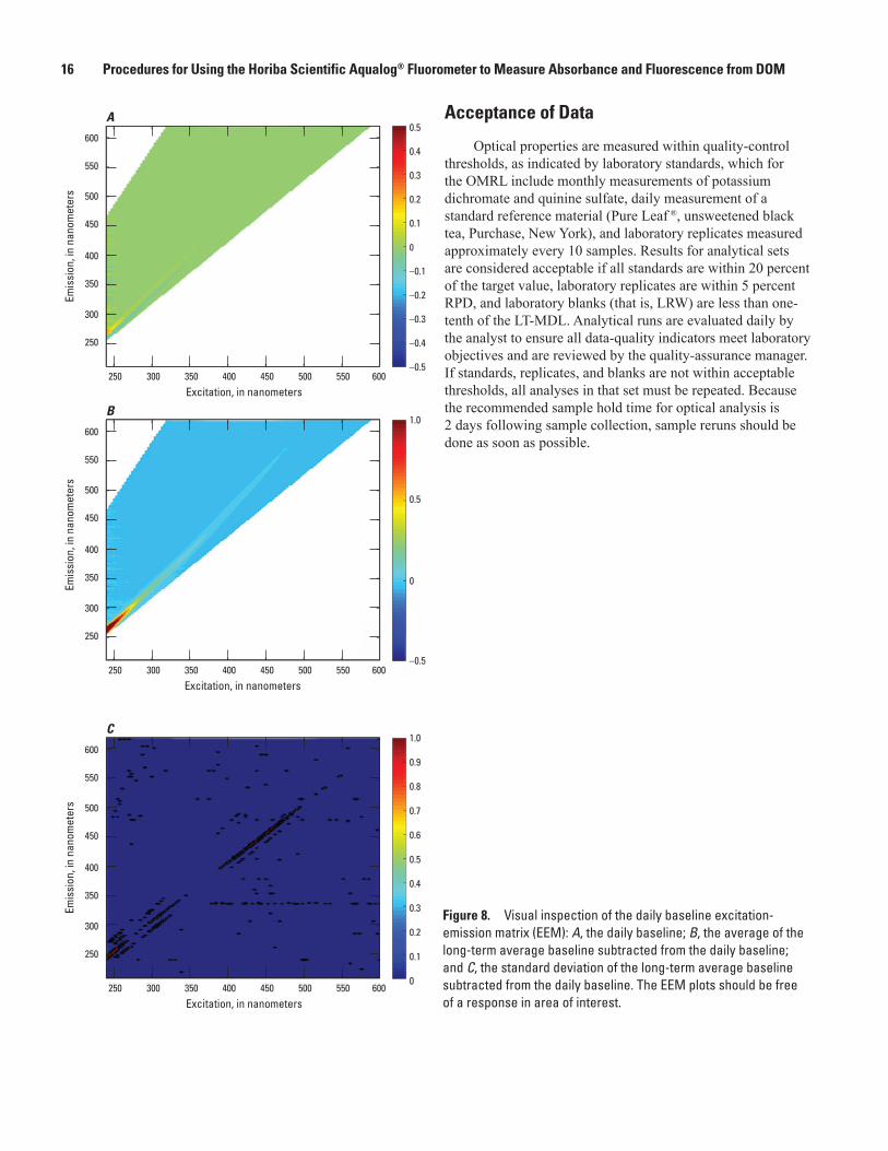
Figure 6. Excitation-emission matrix (EEM) of the standard reference material (Pure Leaf®, unsweetened black tea, Purchase, New York) SRMTea used in the Organic Matter Research Laboratory. The EEM shows the long-term average for SRMTea, which includes 189 scans from 22 lot numbers over a 12-month period. (Labeled regions of the EEM correspond to named peaks or table 1 optical properties; FDOM, fluorescent dissolved organic matter peak.)


Although only a small amount of an 8 ounce (oz) bottle of SRMTea is needed to prepare a standard, each bottle is used only for a maximum of 1 month after opening, with at least 1 week of overlap between old and new bottles. The OMRL lab staff analyzes two different bottles in each analytical run to verify internal consistency before using them as an SRM. Each bottle receives a unique laboratory identifier, and the lot number is recorded for long-term tracking purposes. Although full EEMs are collected for evaluation of performance, internal lab evaluation is tracked for 10 absorbance wavelengths and 8 widely published diagnostic fluorescence ex-em pairs. Acceptance is then based on recovery percentage (plus or minus 20 percent) of the long-term average of the SRM record.

Laboratory Blank SamplesLaboratory blank samples, or blanks, can reveal

background levels and possible contamination of the equipment used during the analytical procedure (for example, cuvette blemishes, improper cuvette rinsing, LRW system quality control). A minimum of 5 laboratory blanks are measured in a typical analytical run; 3 blanks are run prior to running samples, and 2 blanks are run following each set of approximately 10 samples (table 5). Analyzing multiple baseline-corrected laboratory blanks daily allows the analyst to track blank-water quality and instrument drift during the course of the day. Individual blank results are acceptable when absorbance and fluorescence are less than one-tenth of the long-term method detection limit (LT-MDL). Calculating the standard deviation of all blanks in a single analytical run confirms the daily detection limit (DDL) is below the LT-MDL. Although the DDL is not a true detection limit, it serves as a diagnostic tool for daily contamination bias.

Laboratory Sample ReplicatesAnalysis of laboratory sample replicates (aliquots of the

same sample) are a demonstration of precision as measured by the relative percent difference (RPD) between the measurements of the original sample and the replicate sample, calculated as 100 times the absolute difference between the two measurements divided by their average. Laboratory replicates not only check instrument precision, but also reflect the homogeneity of the sample and the precision of the analyst. A minimum of 1 laboratory replicate is measured in a typical analytical run (table 5), where 1 laboratory replicate is measured approximately every 10 samples. Laboratory replicates are considered acceptable when the RPD is less than 5 percent.

Table 5. The scan order for a typical analysis run includes the water Raman, baseline, and analytical set.

[ba, baseline; bl, blank; MMDDYY, month day year; OMRL, Organic Matter Research Laboratory; SRM, standard reference material; —, not applicable]

Scan order

Sample type

File-naming convention

Comments

1 Water Raman wrMMDDYY —2 Baseline baMMDDYY —3 Lab blank blMMDDYYa —4 Lab blank blMMDDYYb —5 Lab blank blMMDDYYc —6 Sample OMRL 1 Sample names should be

unique to the analyzing lab.

7 Sample OMRL 2 —8 Sample OMRL 3 —9 Sample OMRL 4 —

10 Sample OMRL 5 —11 Sample OMRL 6 —12 Sample OMRL 7 —13 Sample OMRL 8 —14 Sample OMRL 9 —15 Sample OMRL 10 —16 SRMTea SRMs01 Tea at 1-percent

concentration. Analyze two SRMs once per day.

17 SRMTea SRMs01 Tea at 1-percent concentration. Analyze two SRMs once per day.

18 Lab replicate OMRL 1d Sample suffix “d” indicates lab replicate.

19 Lab blank blMMDDYYd —20 Lab blank blMMDDYYe A minimum of five blanks

should be run per day.Continue analyzing samples, repeating above sequence from rows

6–20 (do not repeat the SRMs). Always complete the run with a replicate followed by two blanks to ensure quality assurance.


Analysis Procedure

General operational procedures and instrumental parameters essential to the proper execution of the method for analyzing absorbance and fluorescence on the Aqualog® are described here. A detailed description of the CAWSC OMRL standard operating procedure (SOP) is provided in appendix 1.

Initial preparations for sample analysis include warming up the instrument for 1 hour prior to the first scan. Lamp hours are recorded when the instrument is switched on because the lamp degrades over time, and the manufacturer recommends the lamp be replaced either at 1000 hours of use or after 1 year of installation. The OMRL staff replaces the lamp annually regardless of hours of lamp use. Always wear gloves when handling cuvettes and samples for the Aqualog®. All blanks, dilutions, and standards should be prepared using Type I LRW.

A typical analytical run includes three unique experiments: (1) Raman, (2) baseline, and (3) analytical set. The purpose of these experiments, the reagents used, and the Aqualog® experiment parameters used for each are described in table 6. Aqualog® software enables the analyst to create experiment files that contain specific information for the instrument parameters, including the experiment set-up and acquisition type (Horiba Scientific, 2011, page 13-4). Software setup should include creating these files for each of the three unique experiments (that is, water Raman, baseline, and analytical set) to improve run-time efficiency and to avoid inconsistent sample analysis. Further details regarding

the Raman, baseline, and analytical set are given in the following paragraphs.1. Raman scan. It should be emphasized that long-term

stability of the instrument is one of the chief concerns of the manufacturer and the user, and one of the best known methods to achieve this is by performing the daily Raman scan using LRW. Routine examination of the water Raman spectrum serves as an early indicator of the instrument’s integrity. The Raman peak area is used to normalize fluorescence signals, thus producing data in units that can be compared across instruments. This scan should be performed at the start of each analytical run using LRW to verify that the peak location of the water Raman is 397 plus or minus 1 nm (fig. 7). The Raman area is calculated using the baseline-corrected peak boundary definition (Murphy and others, 2011) outside of the Aqualog® user interface and is determined after collecting a baseline scan (see experiment 2) using a processing routine developed by the OMRL staff. In the OMRL, the Raman area is expected to be within 75 percent of the value obtained after the last lamp change. If the Raman peak location and area do not meet acceptance criteria, allow the instrument to warm up for another 30 minutes and repeat the scan. If acceptance criteria continue not to be met, examine common sources of interference or contamination (for example, cuvette blemishes, LRW contamination, lamp alignment) before contacting the manufacturer for technical support.

Table 6. Aqualog® experiments used in a typical analytical run, along with method, parameters, and reagents.

[CCD, charge-coupled device; Em, emission; Ex, excitation; LRW, lab reagent water; NY, New York; SRM, standard reference material; 3D, three-dimensional; =, equal to]

Scan type Aqualog® method Experiment parameters Purpose Reagent

Raman Spectra. Two-dimensional emission spectra

Integration time=10 Accumulation=1 Ex=350 Em=1.64 (should be equivalent to 3D scan) CCD gain=medium Sample only Cuvette position=1

Used to normalize baseline, blanks and samples to the daily LRW.

Type 1 LRW

Baseline 3D. Three-dimensional emission spectra plus absorbance.

Integration time=1Ex=600-240-3Em=1.64CCD gain=mediumBlank/sample setup=blank onlyCuvette position=1

Establishes a daily baseline for the instrument and is used to baseline correct scans (blanks, samples, and standards).

Type 1 LRW

Analytical set

3D. Three-dimensional emission spectra plus absorbance.

Integration time=1Ex=600-240-3Em=1.64CCD gain=mediumBlank/sample setup=blank from fileCuvette position=1

The analytical set includes samples, verification samples (SRMTea or knowns), sample duplicates, and laboratory blanks.

Blank reagent is organic-free Type 1 LRW. Verification sample (SRMTea) reagent is Pure Leaf ®, unsweetened black tea, Purchase, N.Y.


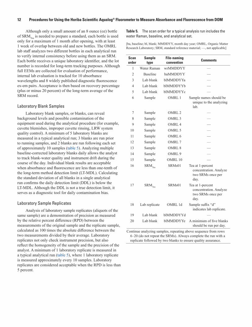
2. Baseline scan. The baseline scan must be collected prior to the analysis of samples to obtain the signal associated with the instrument, cuvette, and LRW in the absence of fluorescent DOM. The daily baseline scan is subtracted from the analytical set collected afterward (see next item). The baseline scan must be quality checked to determine whether it meets laboratory objectives. Quality check the baseline by confirming the response is less than the LT-MDL in the regions of interest. The OMRL staff has developed a processing routine that Raman-normalizes the baseline scan, calculates water Raman area and peak location, and generates three graphs for visual determination of baseline quality (fig. 8). The first graph shows the current baseline scan, the second graph shows the average of the long-term baseline subtracted from the daily baseline, and the third graph shows the difference between the standard deviation of the long-term average baseline and the daily baseline. If the baseline does not pass quality-assurance standards (for example, it exceeds the LT-MDL), allow the instrument to warm up for another 30 minutes and repeat along with the water Raman scan. If acceptance criteria continue not to be met, examine common sources of interference or contamination (for example, cuvette blemishes, LRW contamination) before contacting the manufacturer for technical support.

3. Analytical set. Only after the water Raman and baseline scans have met laboratory-defined objectives should the analytical set begin. An analytical set includes samples, verification samples (that is, SRMTea or knowns), laboratory replicates, and laboratory blanks. A typical analytical set scan order is presented in table 5.

Examination of QA/QC in the analytical set should be done to determine sample reruns and dilution requirements. Fluorescence measurements of highly concentrated samples are subject to measurement errors like detector saturation and inner-filtering effects (IFE). Previous studies indicate the IFE is linear and correctable for most natural samples when A254 is between 0.03–0.3 absorbance units (AU) when measured in a 1 centimeter (cm) cuvette (for example, Ohno, 2002; Lakowicz, 2006, Miller and others, 2010). Most undiluted natural samples from riverine, lake, and estuarine systems far exceed that level, however, as do samples associated with high concentrations of DOM inputs, such as those of wastewater effluent or with oil and gas contamination. To standardize the correction procedure, all samples initially are analyzed at full concentration, and the A255 value is noted. If the A255 exceeds

0.3 AU, the sample is diluted with LRW to a concentration at which the A255 is in the range of 0.03 to 0.3 AU. Note that use of A255 reflects the output of the Aqualog® method for simultaneous collection of fluorescence and absorbance data, where absorbance data are collected in 3-nm increments from 240 to 600 nm.

It should be emphasized that this value of 0.3 AU at A255 was developed for samples containing a “typical” array of DOM compounds (fig. 6); however, samples that have particularly high absorbance and fluorescence in other regions of EEM space may require further dilution to avoid interferences due to IFE or instrument detector saturation in those regions. For example, a sample containing very high fluorescence at low-UV wavelengths could require additional dilution so that the absorbance and fluorescence response falls within a linear range of the instrument across the entire EEMs space.

Data Reporting and Limits

Given there is not a CRM for optical measurements from which to calculate a minimum detection limit (MDL) across the absorbance spectrum or EEM space, the OMRL staff has developed reporting limits by modifying the approach recommended by Childress and others (1999) and the U.S. Environmental Protection Agency (2000). The LT-MDL is reported as three times the standard deviation plus the average of baseline-corrected blanks collected over a 2-year period. Three times the standard deviation is a commonly used estimate of the measured response corresponding to the critical Student’s t value at a significance level of 99 percent, as referenced in Childress and others (1999).

Absorbance LT-MDL was calculated across the spectrum (240–600 nm) from 1200 baseline-corrected instrument blanks analyzed over a 2-year period (January 2013–December 2014). Absorbance is reported in absorbance units (AU) obtained directly from the instrument. Absorbance LT-MDLs vary by wavelength, ranging from 0.01 AU at A240 to 0.004 AU at A600 (fig. 9).

Fluorescence LT-MDL was calculated at each ex-em pair determined from 1200 baseline-corrected, water Raman-normalized blanks collected during the same 2-year period as absorbance (January 2013–December 2014). Fluorescence data are expressed in Raman-normalized intensity units (RU; Murphy and others, 2010). Fluorescence LT-MDLs vary by excitation-emission pairs, ranging from 0.004 RU throughout much of the EEM spectra to 0.1 RU in the region of peak B (ex275, em304; fig. 10).


sac17-0642_fig07ab

1,000

1,500

500

0

2,000

2,500

3,000

375 380 385 390 395 400 405 410 415 420 425

Sign

al h

eigh

t, in

arb

itrar

y un

its

Emission wavelength, in nanometers

A

B

Peak position at emission 397 nanometers

2,000

2,100

2,200

2,300

2,400

2,500

2,600

2,700

2,800

2,900

3,000

Wat

er R

aman

are

a, in

arb

itrar

y un

its

EXPLANATION

Raman areaLamp change

Dec.

7, 2

012

Mar

. 17,

201

3

June

25,

201

3

Oct.

3, 2

013

Jan.

11,

201

4

April

21,

201

4

July

30,

201

4

Nov

. 7, 2

014

Feb.

15,

201

5

May

26,

201

5

Sept

. 3, 2

015

Dec.

12,

201

5

Mar

. 21,

201

6

June

29,

201

6

Oct.

7, 2

016

Figure 7. Aqualog® water Raman criteria: A, peak position should be 397 nanometers plus or minus 1 nanometer; and B, the area should be at least 75 percent of the value obtained after the last lamp change.


sac17-0642_fig08

A

550

600

450

500

350

400

250

250 300 350 400 450 500 550

0.5

0.4

0.3

0.2

0.1

0

–0.1

–0.2

–0.4

–0.3

–0.5600

300


B

550

600

450

500

350

400

250

250 300 350 400 450 500 550

1.0

–0.5

0.5

0

600

300


C

Emis

sion

, in

nano

met

ers

Emis

sion

, in

nano

met

ers

Emis

sion

, in

nano

met

ers

550

600

450

500

350

400

250

250 300 350 400 450 500 550

1.0

0.9

0.8

0.7

0.6

0.5

0.4

0.3

0.2

0.1

0600

300


Figure 8. Visual inspection of the daily baseline excitation-emission matrix (EEM): A, the daily baseline; B, the average of the long-term average baseline subtracted from the daily baseline; and C, the standard deviation of the long-term average baseline subtracted from the daily baseline. The EEM plots should be free of a response in area of interest.

Acceptance of Data

Optical properties are measured within quality-control thresholds, as indicated by laboratory standards, which for the OMRL include monthly measurements of potassium dichromate and quinine sulfate, daily measurement of a standard reference material (Pure Leaf ®, unsweetened black tea, Purchase, New York), and laboratory replicates measured approximately every 10 samples. Results for analytical sets are considered acceptable if all standards are within 20 percent of the target value, laboratory replicates are within 5 percent RPD, and laboratory blanks (that is, LRW) are less than one-tenth of the LT-MDL. Analytical runs are evaluated daily by the analyst to ensure all data-quality indicators meet laboratory objectives and are reviewed by the quality-assurance manager. If standards, replicates, and blanks are not within acceptable thresholds, all analyses in that set must be repeated. Because the recommended sample hold time for optical analysis is 2 days following sample collection, sample reruns should be done as soon as possible.


sac17-0642_fig09

Inte

nsity

, in

abso

rban

ce u

nits


240 260 280 300 320 340 360 380 400 420 440 460 480 500 520 540 560 580 6000.003

0.004

0.005

0.006

0.007

0.008

0.009

0.010

0.011

Figure 9. Absorbance spectra measured between 240 and 600 nanometers indicating the long-term method detection limit calculated using 1200 baseline-corrected blanks analyzed during January 2013–December 2014.

sac17-0642_fig10

280

300

320

340

360

380

400

420

440

460

480

500

520

540

560

580

600

240 260 280 300 320 340 360 380 400 420 440 460 480 500 520 540 560 580 600


Emis

sion

, in

nano

met

ers


0 to 0.150.15>

Figure 10. Fluorescence excitation-emission matrix indicating the long-term method detection limit calculated using 1200 baseline-corrected blanks analyzed January 2013–December 2014.


Data Processing and CorrectionsData processing is performed using processing routines

developed by the OMRL staff. These processing routines are laboratory specific because they are dependent on the sample- and analytical batch-naming conventions and data-storage structure established by the OMRL staff, as well as on the instrument setup and lab-defined QA/QC measurements. A description of the processing and correction of absorbance and fluorescence measurements is given here.

Data organization is paramount for effective processing, retrieval, compilation, and analyses; thus, establishing a consistent file-storage system and standardized sample-naming convention is highly recommended. For reference, an example showing the OMRL folders and files created from one analytical run date (May 18, 2016) is shown in table 7.

All data produced by the Aqualog® using the analysis procedure in this report are instrument- and baseline-corrected. The instrument correction factors account for wavelength-dependent components of the system, like the xenon lamp, gratings, and signal detectors. A set of instrument correction factors—instrument specific and provided by the manufacturer—for excitation (that is, xcorrect.spc) and emission (that is, mcorrect.spc) are automatically applied by the software to each scan (Horiba Scientific, 2011, page 13-2). Baseline correction is applied by the software during analysis, as described previously.

All other data corrections are completed in MATLAB v8.5 R2015a. Performing remaining data treatment outside of the Aqualog® software environment ensures standardization of data and better comparability among datasets and across instruments.

Upon completion of an analytical run, baseline-corrected and instrument-corrected data are exported to the desired storage location using the Aqualog® HJY batch export feature (appendix 1). A MATLAB data processing script developed by OMRL staff then is used to perform corrections (for example, water-Raman normalization, correct for IFE), calculations

(for example, multiply diluted samples to the appropriate concentration, calculate designated slopes and indices), data manipulation (for example, Rayleigh trims, vectorize fluorescence data), compile summary data (for example, extract a subset of widely published absorbance wavelengths, fluorescence ex-em pairs, and indices), evaluate QA data, assign data qualifiers (for example, processed summary reports for absorbance and fluorescence; appendixes 4 and 5, respectively), and manage data structure (for example, add samples to MATLAB structure array where related data types are stored in fields). The OMRL structure array stores complete absorbance spectra and full excitation-emission matrices for all samples analyzed in the laboratory, including all QA/QC samples (for example, daily laboratory blanks, replicates, and SRMTea and monthly Starna potassium dichromate and reference-cell scans). Storage in this type of array allows for easy data retrieval for modeling and reporting.

Data StorageThe Aqualog® collects high-resolution scans that include

thousands of individual datum points for each sample; thus, data storage is not trivial. The OMRL staff archives the raw-data files and processed-data files on an internal network server. These files are available upon request and include the Aqualog® software project file; original exported data files including baseline, water Raman, sample and blank scans; and processed files containing full-absorbance scans, fluorescence EEMs, and laboratory QA data.

Only a subset of these data from selected projects and samples for which sites have been established are available to the public through the USGS National Water Information System (NWIS); these are limited to the commonly published diagnostic parameters and indices listed in table 8. The diagnostic wavelengths and EEMs pairs are transferred to the OMRL internal database when all QA/QC have been evaluated and accepted.

Data Storage 19

Aqualog - DOM

– Aqua DOM 2016– q2016-05-18

– Exported Aqualog Files– qa2016-05-18

– bl051816a.csvbl051816b.csvbl051816c.csvbl051816d.csvbl051816e.csvgr20329.csvgr20329d.csvgr20330.csvgr20331.csvgr20332.csvgr20332s50.csvgr20334.csvgr20335.csvgr20335s50.csvgr20336.csvgr20336s10.csvgr20337.csvgr20338.csvgr20339.csvgrSRMHTs01.csvgrSRMHUs01.csv

Aqualog - DOM

– Aqua DOM 2016—Continued– q2016-05-18—Continued

– Exported Aqualog Files—Continued– qf2016-05-18

bl051816a.datbl051816b.datbl051816c.datbl051816d.datbl051816e.datgr20329.datgr20329d.datgr20330.datgr20331.datgr20332.datgr20332s50.datgr20334.datgr20335.datgr20335s50.datgr20336.datgr20336s10.datgr20337.datgr20338.datgr20339.datgrSRMHTs01.datgrSRMHUs01.datwr051816.dat

Table 7. The Organic Matter Research Laboratory data-storage structure for example analysis date of May 18, 2016.

[Files are in alpha-numeric order. Sample suffix “s” followed by numbers denotes diluted sample percent concentration. Sample suffix “d” indicates a laboratory replicate scan. File extension .csv indicates a comma-separated file and .dat indicates a generic data file created upon export by Aqualog software. Abbreviation: DOM, dissolved organic matter]


Table 8. National Water Information System (NWIS) codes for commonly published diagnostic parameters and indices.

[cm, centimeter; em, emission; ex, excitation; FDOM, fluorescent dissolved organic matter; nm, nanometer; RU, Raman units; UV, ultraviolet; wf, filtered water]

Method tool Analyte Result name Parameter definitionMethod

codeParameter

code

Horiba Scientific Aqualog®

Absorbance A254 Absorbance, 254 nm, water, filtered, absorbance units per centimeter.

UV008 50624


Absorbance SUVA254 Specific UV absorbance, 254 nm, water, filtered, 1-cm path length, calculated, liter per milligram of dissolved organic carbon per meter.

UV003 63162


Absorbance A280 Absorbance at 280 nm, water, filtered, absorbance units per centimeter.

ABS01 32296



ABS01 32297



ABS01 32298



ABS01 32299


Absorbance S275–295 Absorption spectral slope, wavelengths 275–295 nm, unitless.

ABS02 32300



ABS02 32301



ABS02 32302



ABS02 32331


Fluorescence Peak A Fluorescence, wf, ex260 em450 RU. FL020 32304


Fluorescence Peak B Fluorescence, wf, ex275 em304 RU. FL020 32305


Fluorescence Peak C Fluorescence, wf, ex340 em440 RU. FL020 52901


Fluorescence Peak D Fluorescence, wf, ex390 em510 RU. FL020 32307


Fluorescence FDOM Fluorescence, wf, ex370 em460 RU. FL020 52902


Fluorescence Peak M Fluorescence, wf, ex300 em390 RU. FL020 32309


Fluorescence Peak N Fluorescence, wf, ex280 em370 RU. FL020 32310


Fluorescence Peak T Fluorescence, wf, ex275 em340 RU. FL020 32311


Fluorescence FI Fluorescence index—ratio of emission intensities that characterizes the slope of the emission curve at an excitation of 370 nm.

FL020 32312


Fluorescence HIX Humification index—calculated by dividing the fluorescence intensity in the 435–480 nm region by the total intensities in the 300–345 and 435–480 nm regions.

FL020 32313

Data Analysis 21

Data AnalysisThe approach to optical data analysis depends on the

objective of the study and the scale of measurement (that is, quantitative or qualitative). As mentioned before and described in table 1, discrete diagnostic wavelengths and indices can be extracted from the absorbance and fluorescence scans. In addition, multi-parameter techniques can be used that incorporate all the data (that is, complete absorbance spectra and fluorescence matrices). A brief overview of some of the ways optical measurements of DOM have been used, with a focus on approaches used by the OMRL staff, is provided here. For additional information, the reader is referred to an extensive body of literature on this topic (Coble, 1996; McKnight and others, 2001; Stedmon and others, 2003; Fellman and others, 2010; Coble and others, 2014).

The measurement of ultraviolet absorbance has been used by the drinking-water industry for decades and has been shown to be a useful proxy for DOC concentration (that is, A254; Edzwald and others, 1985; Rathbun, 1996; Korshin and others, 1997; Sadiq and Rodriguez, 2004) and disinfection byproduct (DBP) precursor concentrations (that is, A272; Korshin and others, 2002; Li and others, 2002; Roccaro and others, 2008). In addition to concentration, absorbance data can provide insight into the chemical composition of the DOM pool. Carbon normalization of the intensity of the response at a given absorbance wavelength (that is, SUVA254 calculated as A254 value divided by DOC concentration, reported in L/mg C/m) has been shown to be correlated with the hydrophobic organic acid fraction of DOM (Spencer and others, 2012) and is a useful proxy for DOM aromatic content (Weishaar and others, 2003) and molecular weight (Chowdhury, 2013). Similarly, spectral slopes and slope ratios have been related to the relative molecular weight and aromaticity of DOM (Chin and others, 1994; Helms and others, 2008); lower values are generally indicative of higher molecular weight DOM, which can change upon photolytic exposure (Helms and others, 2008; Spencer and others, 2009; Hansen and others, 2016).

Fluorescence intensity at a given ex-em pair also can be related to DOC concentration, DBP precursor concentrations (Kraus and others, 2010; Beggs and Summers, 2011; Carpenter and others, 2013), biological oxygen demand (Baker and Curry, 2004; Hudson and others, 2008), mercury concentrations (Fleck and others, 2014), and wastewater content (Goldman and others, 2012). Like absorbance data, fluorescence data also are widely used to gain insight into DOM composition, source, and reactivity. Information about DOM composition can be inferred from the presence or absence of fluorophores, shifts in peak maxima, ratios of peaks, and calculated indices, as well as by normalizing each ex-em pair by DOC concentration (Beggs and Summers, 2011). Commonly reported DOM compositional indicators include the fluorescence index, humification index, freshness index, and biological index (table 1).

Although these diagnostic wavelengths and indices can be very informative, they often miss information that can be

gleaned by using the full absorbance and fluorescence dataset generated by instruments like the Aqualog®. Other approaches to data interpretation involve the use of multivariate and multi-way modeling techniques (Stedmon and others, 2003; Fellman and others, 2008). In the following paragraphs, we discuss three commonly used approaches—principal component analysis (PCA), discriminant analysis (DA), and parallel factor analysis (PARAFAC)—and then provide more detailed information about tools the OMRL staff have developed to run PARAFAC.

Principal component analysis (PCA) is one of the most frequently used multivariate techniques to explore optical data (for example, Stepanauskas and others, 2003; Baker and others, 2008; Jaffé and others, 2008; Kraus and others, 2008; Dalzell and others, 2009; Miller and McKnight, 2010; Goldman and others, 2012, 2014). The primary aim of PCA is dimension reduction, in which uncorrelated linear combinations called principal components are identified. The first component explains the most variability in a dataset, the second component explains the second-most, and so on. Model output displays scores (clustering and/or separation of objects and their relationship to the principal components) and loadings (the original loadings projected onto the principal axes; fig. 11).

Discriminant analysis (DA) is a predictive method that classifies a sample to a user-designated group on the basis of known responses. Although DA is performed more rarely than PCA, it has potential to improve our understanding of DOM biogeochemical processes because of its ability to analyze complex spatial relationships, and it allows for the identification of the most important discriminating variables that lead to proper assignment of a sample to a designated group (for example, Spencer and others, 2007; Hansen and others, 2016; fig. 12).

Parallel factor analysis (PARAFAC), a multi-way statistical approach for detecting underlying structures in complex datasets like fluorescence EEMs, has proven to be a powerful tool for studying DOM (Bro, 1997) and has been widely applied in combination with other measurements to rapidly quantify and characterize DOM across a range of environments (for example, Stedmon and Markager, 2005; Fellman and others, 2008; Kowalczuk and others, 2009). The aim of PARAFAC is to distill fluorescence signatures into distinct fluorescence components (fluorophores) that are not restricted to a single excitation-emission pair.

Unlike PCA or DA, which are common statistical methods available in many software packages (for instance, OMRL uses SAS JMP v.12.2) PARAFAC requires the use of MATLAB, or a similar high-performance programming language (for example, Python or R), that allows users to perform matrix calculations, develop and run algorithms, and create data visualization products and user interfaces.

In order to run PARAFAC in MATLAB, the data structure must be arranged in a specific format according to the procedures in Stedmon and Bro (2008).


PARAFAC model validation is determined by examining a variety of methods in combination (for example, analysis of spectral properties, split-half analysis, residual analysis, and random initialization). Although there is no quantitative measure of “best fit” (Murphy and others, 2013), subjectivity in determining the final modeled components can be minimized by evaluating each dataset carefully using the diverse validation methods explained by Stedmon and Bro (2008).

When validated, component loadings are interpreted to represent individual fluorophores and can be examined

by the absolute value (that is, component loadings), which is a reflection of the intensity of fluorescence, and by the relative contribution to total fluorescence (that is, component percentage loadings), which is a reflection of composition (fig. 13). Model component loadings can be used for further analysis of the individual observations like “new parameters” in other multivariate approaches discussed previously, such as PCA (for example, Kraus and others, 2008; Miller and McKnight 2010; Fleck and others, 2014) or DA (Spencer and others, 2007; Hansen and others, 2016), to gain insight into DOM composition.

sac17-0642_fig11

A B

–4

–3

–2

–1

0

1

2

3

4

Com

pone

nt 2

(17

.1%

)

–4 –3 3–2 –1 1 20 4

Component 1 (40.9%)

–1.0

–0.5

0.0

0.5

1.0

Com

pone

nt 2

(17

.1%

)

S350–400S350–400

–1.0 –0.5 0.0 0.5 1.0

Component 1 (40.9%)

C:MC:M

SVA555SVA555

C:AC:AS275–295S275–295

FIFI

β:αβ:α

EXPLANATION

Study unit A

Study unit B

Study unit C

Study unit D

Study unit E

Figure 11. Example of model output from principal component analysis: A, the score plot displays clustering or separation of individual samples and their relationship to the principal components; and B, the loadings plot graphs the original loadings projected onto the principal axes. (Original loadings correspond to selected optical measurements, labels abbreviated as in table 1.)

Data Analysis 23

sac17-0642_fig12

SVA555

S275–295

S350–400S350–400

FI

C:A

C:Mβ:α

Canonical 1

EXPLANATION

Study unit A Abbreviations

Study unit B

Study unit C

Study unit D

Study unit E

S

C:A

SVA

C:M

Fl

Slope

Fluorescence ratio of Peak to Peak A

Specific visible absorbance

Fluorescence ratio of Peak to Peak M

Fluorescence

–8

–6

–4

–2

0

2

4

6

8

Cano

nica

l 2

–8 –6 –4 –2 2 4 6 80

Stud

y un

it D

Stud

y un

it D

Stud

y un

it A

Stud

y un

it A

Stud

y un

it C

Stud

y un

it C

Stud

y un

it B

Stud

y un

it B

Stud

y un

it E

Stud

y un

it E

Figure 12. Example of model output from discriminant analysis. The canonical plot shows the two dimensions (canonicals 1 and 2) that provide the best separation among user-defined groups. Points are individual samples; inner ellipses represent the 95-percent confidence interval for group means and outer ellipses represent the region estimated to contain 50 percent of the population of each group; and the biplot ray represents the covariates and the degree of association of the covariates with the two canonical variables.


sac17-0642_fig13

A

B

C

Inte

nsity

, in

Ram

an u

nits

Com

posi

tion,

in p

erce

nt

Sample number

00 50 100 200 250150

20

40

60

80

100

0

0.1

0.2

0.3

0.4

0.5

Component 1

300250 350Excitation, in nanometers

Emis

sion

, in

nano

met

ers

400 450

550

450

350

300

400

600

500

Component 2 Component 3 Component 4 Component 5


400 450

550

450

350

300

400

600

500


400 450

550

450

350

300

400

600

500


400 450

550

450

350

300

400

600

500


400 450

550

450

350

300

400

600

500

EXPLANATIONModel loadings

Component 1Component 2Component 3Component 4Component 5

EXPLANATIONModel loadings

Component 1Component 2Component 3Component 4Component 5

0.22

0.18

0.14

0.01

0.06

0.02 Inte

nsity

, in

Ram

an u

nits

Figure 13. Example of model output from parallel factor analysis (PARAFAC): A, component loadings are interpreted to represent individual fluorophores and can be examined; B, by absolute value, which is a reflection of the intensity of fluorescence; and C, by the relative contribution to total fluorescence, which is a reflection of composition.

References Cited 25

SummaryThe purpose of this document is to provide a standardized

method for the collection, correction, and interpretation of optical data produced by the Aqualog®. Optical measurements such as absorbance and fluorescence are easy to take; however, they can be affected by many variables rendering them less comparable, including such things as inconsistencies in sample collection (for example, filter pore size, preservation), the application of corrections for interferences (for example, inner-filtering corrections), differences in holding times, and instrument drift (for example, lamp intensity). A documented, standardized procedure to address these variables ensures that the optical (absorbance and fluorescence) measurements collected by U.S. Geological Survey (USGS) researchers are useful and widely comparable.

Rigorous and quantifiable quality assurance and quality control are essential for making these data comparable, particularly because there is no published guideline for the measurement of dissolved organic matter (DOM) absorbance and fluorescence, and especially because there is no National Institute of Standards and Technology standard for DOM. Validation and quality-control samples are analyzed on a monthly basis to determine laboratory and instrument precision and daily (that is, each day samples are run) to ensure repeatability. Data are not considered acceptable unless they meet laboratory criteria: All standards should be within 20 percent of the target value, laboratory replicates should be within 5 percent relative percent difference, and laboratory blanks (that is, laboratory reagent-grade water) should be less than one-tenth of the long-term method detection limit.

Finally, for data to be useful, they must be accessible to users in a format that can be easily analyzed and interpreted. The Organic Matter Research Laboratory staff has developed a processing routine that extracts a subset of the data, which is made available to the public through the USGS National Water Quality Information System (http://nwis.waterdata.usgs.gov/usa/nwis/qwdata), and organizes the full datasets (that is, complete absorbance spectra and fluorescence excitation-emission matrices) in different forms that allow for these data to be analyzed using multi-parameter and multi-way statistical approaches.

AcknowledgmentsWe thank Erica DeParsia, Amaryl Griggs,

Quratulain Ahmed, and Sydney Berrios for laboratory assistance and logistical support. We appreciate reviews provided by Peter Lenaker and Emily Woodward which improved the quality and presentation of this work. Funding was provided by the California Water Science Center, Sacramento, California.

References Cited

Baker, A., and Curry, M.P., 2004, Fluorescence of leachates from three contrasting landfills: Water Research, v. 38, no. 10, p. 2605–2613, https://doi.org/10.1016/j.watres.2004.02.027.

Baker, A., and Spencer, R.G.M., 2004, Characterization of dissolved organic matter from source to sea using fluorescence and absorbance spectroscopy: Science of the Total Environment, v. 333, no. 1–3, p. 217–232, https://doi.org/10.1016/j.scitotenv.2004.04.013.

Baker, A., Elliott, S., and Lead, J.R., 2007, Effects of filtration and pH perturbation on freshwater organic matter fluorescence: Chemosphere, v. 67, no. 10, p. 2035–2043, https://doi.org/10.1016/j.chemosphere.2006.11.024.

Baker, A., Bolton, L., Newson, M.D., and Spencer, R.G.M., 2008, Spectrophotometric properties of surface water dissolved organic matter in an afforested upland peat catchment: Hydrological Processes, v. 22, no. 13, p. 2325–2336, https://doi.org/10.1002/hyp.6827.

Beggs, K.M.H., and Summers, R.S., 2011, Character and chlorine reactivity of dissolved organic matter from a mountain pine beetle impacted watershed: Environmental Science and Technology, v. 45, no. 13, p. 5717–5724, https://doi.org/10.1021/es1042436.

Blough, N.V., and Del Vecchio, R., 2002, Chromophoric DOM in the coastal environment, chap. 10 in Hansell, D.A., and Carlson, C.A., eds., Biogeochemistry of marine dissolved organic matter: Academic Press, p. 509–546, https://doi.org/10.1016/B978-012323841-2/50012-9.

Bro, R., 1997, PARAFAC. Tutorial and applications: Chemometrics and Intelligent Laboratory Systems, v. 38, no. 2, p. 149–171, https://doi.org/10.1016/S0169-7439(97)00032-4.

Burdige, D.J., Kline, S.W., and Chen, W.H., 2004, Fluorescent dissolved organic matter in marine sediment pore waters: Marine Chemistry, v. 89, no. 1–4, p. 289–311, https://doi.org/10.1016/j.marchem.2004.02.015.

Carpenter, K.D., Kraus, T.E.C., Goldman, J.H., Saraceno, J.F., Downing, B.D., Bergamaschi, B.A., McGhee, G., and Triplett, T., 2013, Sources and characteristics of organic matter in the Clackamas River, Oregon, related to the formation of disinfection by-products in treated drinking water: U.S. Geological Survey Scientific Investigations Report 2013–5001, 78 p., https://pubs.usgs.gov/sir/2013/5001/.



https://doi.org/10.1016/j.watres.2004.02.027

https://doi.org/10.1016/j.scitotenv.2004.04.013

https://doi.org/10.1016/j.chemosphere.2006.11.024

https://doi.org/10.1002/hyp.6827

https://doi.org/10.1021/es1042436

https://doi.org/10.1016/B978-012323841-2/50012-9

https://doi.org/10.1016/S0169-7439(97)00032-4

https://doi.org/10.1016/j.marchem.2004.02.015

https://pubs.usgs.gov/sir/2013/5001/


Carstea, E.M., Ghervase, L., Pavelescu, G., and Savastru, D., 2009, Assessment of the anthropogenic impact on water systems by fluorescence spectroscopy: Environmental Engineering and Management Journal, v. 8, no. 6, p. 1321–1326.

Childress, C.J.O., Foreman, W.T., Connor, B.F., and Maloney, T.J., 1999, New reporting procedures based on long-term method detection levels and some considerations for interpretations of water-quality data provided by the U.S. Geological Survey National Water Quality Laboratory: U.S. Geological Survey Open-File Report 99–193, 19 p., https://pubs.er.usgs.gov/publication/ofr99193.

Chin, Y.-P., Aiken, G., and O’Loughlin, E., 1994, Molecular weight, polydispersity, and spectroscopic properties of aquatic humic substances: Environmental Science and Technology, v. 28, no. 11, p. 1853–1858, https://doi.org/10.1021/es00060a015.

Chowdhury, S., 2013, Trihalomethanes in drinking water—Effect of natural organic matter distribution: Water SA, v. 39, no. 1, p. 1–7, https://www.ajol.info/index.php/wsa/article/view/87900.

Coble, P.G., 1996, Characterization of marine and terrestrial DOM in seawater using excitation-emission matrix spectroscopy: Marine Chemistry, v. 51, no. 4, p. 325–346, https://doi.org/10.1016/0304-4203(95)00062-3.

Coble, P.G., 2007, Marine optical biogeochemistry—The chemistry of ocean color: Chemical Reviews, v. 107, no. 2, p. 402–418, https://doi.org/10.1021/cr050350%2B.

Coble, P.G., Lead, J., Baker, A., Reynolds, D.M., and Spencer, R.G.M., 2014, Aquatic organic matter fluorescence, part of Cambridge Enviornmental Chemistry Series: New York, N.Y., Cambridge University Press, 375 p.

Cory, R.M., Miller, M.P., McKnight, D.M., Guerard, J.J., and Miller, P.L., 2010, Effect of instrument-specific response on the analysis of fulvic acid fluorescence spectra: Limnology and Oceanography: Methods, v. 8, no. 2, p. 67–78, https://doi.org/10.4319/lom.2010.8.67.

Dalzell, B.J., Minor, E.C., and Mopper, K.M., 2009, Photodegradation of estuarine dissolved organic matter—A multi-method assessment of DOM transformation: Organic Geochemistry, v. 40, no. 2, p. 243–257, https://doi.org/10.1016/j.orggeochem.2008.10.003.

Downing, B.D., Boss, E., Bergamaschi, B.A., Fleck, J.A., Lionberger, M.A., Ganju, N.K., Schoellhamer, D.H., and Fujii, R., 2009, Quantifying fluxes and characterizing compositional changes of dissolved organic matter in aquatic systems in situ using combined acoustic and optical measurements: Limnology Oceanography: Methods, v. 7, no. 1, p. 119–131, https://doi.org/10.4319/lom.2009.7.119.

Edzwald, J.K., Becker, W.C., and Wattier, K.L., 1985, Surrogate parameters for monitoring organic matter and THM precursors: Journal of American Water Works Association, v. 77, no. 4, p. 122–132, http://www.jstor.org/stable/41272390.

Fellman, J.B., D’Amore, D.V., Hood, E., and Boone, R.D., 2008, Fluorescence characteristics and biodegradability of dissolved organic matter in forest and wetland soils from coastal temperate watersheds in southeast Alaska: Biogeochemistry, v. 88, no. 2, p. 169–184.

Fellman, J.B., Hood, E., and Spencer, R.G.M., 2010, Fluorescence spectroscopy opens new windows into dissolved organic matter dynamics in freshwater ecosystems—A review: Limnology and Oceanography, v. 55, no. 6, p. 2452–2462, https://doi.org/10.4319/lo.2010.55.6.2452.

Fleck, J.A., Gill, G., Bergamaschi, B.A., Kraus, T.E.C., Downing, B.D., and Alpers, C.N., 2014, Concurrent photolytic degradation of aqueous methylmercury and dissolved organic matter: Science of the Total Environment, v. 484, p. 263–275, https://doi.org/10.1016/j.scitotenv.2013.03.107.

Goldman, J.H., Rounds, S.A., and Needoba, J.A., 2012, Applications of fluorescence spectroscopy for predicting percent wastewater in an urban stream: Environmental Science and Technology, v. 46, no. 8, p. 4374–4381, https://doi.org/10.1021/es2041114.

Goldman, J.H., Rounds, S.A., Keith, M.K., and Sobieszczyk, S., 2014, Investigating organic matter in Fanno Creek, Oregon, Part 3 of 3—Identifying and quantifying sources of organic matter to an urban stream: Journal of Hydrology, part D in v. 519, p. 3028–3041, https://doi.org/10.1016/j.jhydrol.2014.07.033.

Hansen, A.M., Kraus, T.E.C., Pellerin, B.A., Fleck, J.A., Downing, B.D., and Bergamaschi, B.A., 2016, Optical properties of dissolved organic matter (DOM)—Effects of biological and photolytic degradation: Limnology and Oceanography, v. 61, no. 3, p. 1015–1032, https://doi.org/10.1002/lno.10270.

Hansen, A.M., Kraus, T.E.C., Bachand, S.M., Horwath, W.R., and Bachand, P.A.M., 2018, Wetlands receiving water treated with coagulants improve water quality by removing dissolved organic carbon and disinfection byproduct precursors: Science of The Total Environment, v. 622–623, p. 603–613, https://doi.org/10.1016/j.scitotenv.2017.11.205.

Helms, J.R., Stubbins, A., Ritchie, J.D., Minor, E.C., Kieber, D.J., and Mopper, K., 2008, Absorption spectral slopes and slope ratios as indicators of molecular weight, source, and photobleaching of chromophoric dissolved organic matter: Limnology and Oceanography, v. 53, no. 3, p. 955–969, https://doi.org/10.4319/lo.2008.53.3.0955.

https://pubs.er.usgs.gov/publication/ofr99193

https://doi.org/10.1021/es00060a015

https://www.ajol.info/index.php/wsa/article/view/87900

https://doi.org/10.1016/0304-4203(95)00062-3

https://doi.org/10.1021/cr050350%2B

https://doi.org/10.4319/lom.2010.8.67

https://doi.org/10.1016/j.orggeochem.2008.10.003

https://doi.org/10.4319/lom.2009.7.119

http://www.jstor.org/stable/41272390

https://doi.org/10.4319/lo.2010.55.6.2452


https://doi.org/10.1021/es2041114

https://doi.org/10.1016/j.jhydrol.2014.07.033

https://doi.org/10.1002/lno.10270


https://doi.org/10.4319/lo.2008.53.3.0955

References Cited 27

Helms, J.R., Stubbins, A., Perdue, E.M., Green, N.W., Chen, H., and Mopper, K., 2013, Photochemical bleaching of oceanic dissolved organic matter and its effect on absorption spectral slope and fluorescence: Marine Chemistry, v. 155, p. 81–91.

Hernes, P.J., Bergamaschi, B.A., Eckard, R.S., and Spencer, R.G.M., 2009, Fluorescence-based proxies for lignin in freshwater dissolved organic matter: Journal of Geophysical Research—Biogeosciences, v. 114, 10 p., https://doi.org/10.1029/2009JG000938.

Horiba Scientific, 2011, AquaLog® Operation Manual, AquaLog®, Part number J810012 rev. E, October 3, 2013, 262 p., http://www.horiba.com.

Hudson, N., Baker, A., Ward, D., Reynolds, D.M., Brunsdon, C., Carliell-Marquet, C., and Browning, S., 2008, Can fluorescence spectrometry be used as a surrogate for the biochemical oxygen demand (BOD) test in water quality assessment? An example from South West England: Science of the Total Environment, v. 391, no. 1, p. 149–158, https://doi.org/10.1016/j.scitotenv.2007.10.054.

Hudson, N., Baker, A., Reynolds, D.M., Carliell-Marquet, C., and Ward, D., 2009, Changes in freshwater organic matter fluorescence intensity with freezing/thawing and dehydration/rehydration: Journal of Geophysical Research—Biogeosciences, v. 114, no. G4, 11 p., https://doi.org/10.1029/2008JG000915.

Huguet, A., Vacher, L., Relexans, S., Saubusse, S., Froidefond, J.M., and Parlanti, E., 2009, Properties of fluorescent dissolved organic matter in the Gironde Estuary: Organic Geochemistry v. 40, no. 6, p. 706–719, https://doi.org/10.1016/j.orggeochem.2009.03.002.

Jaffé, R., McKnight, D., Maie, N., Cory, R., McDowell, W.H., and Campbell, J.L., 2008, Spatial and temporal variations in DOM composition in ecosystems—The importance of long-term monitoring of optical properties: Journal of Geophysical Research—Biogeosciences, v. 113, no. G4, 15 p., https://doi.org/10.1029/2008JG000683.

Korshin, G.V., Li, C.-W., and Benjamin, M.M., 1997, Monitoring the properties of natural organic matter through UV spectroscopy—A consistent theory: Water Research, v. 31, no. 7, p. 1787–1795, https://doi.org/10.1016/S0043-1354(97)00006-7.

Korshin, G.V., Wu, W.W., Benjamin, M.M., and Hemingway, O., 2002, Correlations between differential absorbance and the formation of individual DBPs: Water Research, v. 36, no. 13, p. 3273–3282, https://doi.org/10.1016/S0043-1354(02)00042-8.

Kowalczuk, P., Durako, M.J., Young, H., Kahn, A.E., Cooper, W.J., and Gonsior, M., 2009, Characterization of dissolved organic matter fluorescence in the South Atlantic Bight with use of PARAFAC model—Interannual variability: Marine Chemistry, v. 113, no. 3–4, p. 182–196, https://doi.org/10.1016/j.marchem.2009.01.015.

Kraus, T.E.C., Bergamaschi, B.A., Hernes, P.J., Spencer, R.G.M., Stepanauskas, R., Kendall, C., Losee, R.F., and Fujii, R., 2008, Assessing the contribution of wetlands and subsided islands to dissolved organic matter and disinfection byproduct precursors in the Sacramento–San Joaquin River Delta—A geochemical approach: Organic Geochemistry, v. 39, no. 9, p. 1302–1318, https://doi.org/10.1016/j.orggeochem.2008.05.012.

Kraus, T.E.C., Anderson, C.A., Morgenstern, K., Downing, B.D., Pellerin, B.A., and Bergamaschi, B.A., 2010, Determining sources of dissolved organic carbon and disinfection byproduct precursors to the McKenzie River, Oregon: Journal of Environmental Quality, v. 39, no. 6, p. 2100–2112, https://doi.org/10.2134/jeq2010.0030.

Lakowicz, J.R., 2006, Principles of fluorescence spectroscopy (3d ed.): Springer Science and Business Media, 954 p.

Lapierre, J.-F., and Frenette, J.-J., 2009, Effects of macrophytes and terrestrial inputs on fluorescent dissolved organic matter in a large river system: Aquatic Sciences, v. 71, no. 1, p. 15–24.

Li, C., Benjamin, M.M., and Korshin, G.V., 2002, The relationship between TOX formation and spectral changes accompanying chlorination of pre-concentrated or fractionated NOM: Water Research, v. 36, no. 13, p. 3265–3272, https://doi.org/10.1016/S0043-1354(02)00020-9.

McKnight, D.M., Boyer, E.W., Westerhoff, P.K., Doran, P.T., Kulbe, T., and Andersen, D.T., 2001, Spectrofluorometric characterization of dissolved organic matter for indication of precursor organic material and aromaticity: Limnology and Oceanography, v. 46, no. 1, p. 38–48, https://doi.org/10.4319/lo.2001.46.1.0038.

Miller, M.P., and McKnight, D.M., 2010, Comparison of seasonal changes in fluorescent dissolved organic matter among aquatic lake and stream sites in the Green Lakes Valley: Journal of Geophysical Research—Biogeosciences, v. 115, no. G1, 14 p., https://doi.org/10.1029/2009JG000985.

Miller, M.P., Simone, B.E., McKnight, D.M., Cory, R.M., Williams, M.W., and Boyer, E.W., 2010, New light on a dark subject—Comment: Aquatic Sciences, v. 72, no. 3, p. 269–275.

https://doi.org/10.1029/2009JG000938

http://www.horiba.com


https://doi.org/10.1029/2008JG000915


https://doi.org/10.1029/2008JG000683

https://doi.org/10.1016/S0043-1354(97)00006-7

https://doi.org/10.1016/S0043-1354(02)00042-8

https://doi.org/10.1016/j.marchem.2009.01.015


https://doi.org/10.2134/jeq2010.0030

https://doi.org/10.1016/S0043-1354(02)00020-9

https://doi.org/10.4319/lo.2001.46.1.0038

https://doi.org/10.1029/2009JG000985


Mobed, J.J., Hemmingsen, S.L., Autry, J.L., and McGown, L.B., 1996, Fluorescence characterization of IHSS humic substances—Total luminescence spectra with absorbance correction: Environmental Science and Technology, v. 30, no. 10, p. 3061–3065, https://doi.org/10.1021/es960132l.

Moran, M.A., Sheldon, W.M. Jr., and Zepp, R.G., 2000, Carbon loss and optical property changes during long-term photochemical and biological degradation of estuarine dissolved organic matter: Limnol Oceanography, v. 45, no. 6, p. 1254–1264, https://doi.org/10.4319/lo.2000.45.6.1254.

Murphy, K.R., Butler, K.D., Spencer, R.G.M., Stedmon, C.A., Boehme, J.R., and Aiken, G.R., 2010, Measurement of dissolved organic matter fluorescence in aquatic environments—An interlaboratory comparison: Environmental Science and Technology, v. 44, no. 24, p. 9405–9412, https://doi.org/10.1021/es102362t.

Murphy, K.R., Hambly, A., Singh, S., Henderson, R.K., Baker, A., Stuetz, R., and Khan, S.J., 2011, Organic matter fluorescence in municipal water recycling schemes—Toward a unified PARAFAC model: Environmental Science and Technology, v. 45, no. 7, p. 2909–2916, https://doi.org/10.1021/es103015e.

Murphy, K.R., Stedmon, C.A., Graeber, D., and Bro, R., 2013, Fluorescence spectroscopy and multi-way techniques—PARAFAC: Analytical Methods, v. 5, no. 23, p. 6557–6566, https://doi.org/10.1039/C3AY41160E.

Ohno, T., 2002, Fluorescence inner-filtering correction for determining the humification index of dissolved organic matter: Environmental Science and Technology, v. 36, no. 4, p. 742–746, https://doi.org/10.1021/es0155276.

Para, J., Coble, P.G., Charrière, B., Tedetti, M., Fontana, C., and Sempéré, R., 2010, Fluorescence and absorption properties of chromophoric dissolved organic matter (CDOM) in coastal surface waters of the northwestern Mediterranean Sea, influence of the Rhône River: Biogeosciences, v. 7, no. 12, p. 4083–4103, https://doi.org/10.5194/bg-7-4083-2010.

Parlanti, E., Worz, K., Geoffroy, L., and Lamotte, M., 2000, Dissolved organic matter fluorescence spectroscopy as a tool to estimate biological activity in a coastal zone submitted to anthropogenic inputs: Organic Geochemistry, v. 31, no. 12, p. 1765–1781, https://doi.org/10.1016/S0146-6380(00)00124-8.

Rathbun, R.E., 1996, Regression equations for disinfection by-products for the Mississippi, Ohio and Missouri rivers: Science of the Total Environment, v. 191, no. 3, p. 235–244, https://doi.org/10.1016/S0048-9697(96)05266-7.

Roccaro, P., Chang, H.-S., Vagliasindi, F.G.A., and Korshin, G.V., 2008, Differential absorbance study of effects of temperature on chlorine consumption and formation of disinfection by-products in chlorinated water: Water Research, v. 42, no. 8–9, p. 1879–1888, https://doi.org/10.1016/j.watres.2007.11.013.

Sadiq, R., and Rodriguez, M.J., 2004, Disinfection by-products (DBPs) in drinking water and predictive models for their occurrence—A review: Science of the Total Environment, v. 321, no. 1–3, p. 21–46, https://doi.org/10.1016/j.scitotenv.2003.05.001.

Spencer, R.G.M., Pellerin, B.A., Bergamaschi, B.A., Downing, B.D., Kraus, T.E.C., Smart, D.R., Dahlgren, R.A., and Hernes, P.J., 2007, Diurnal variability in riverine dissolved organic matter composition determined by in situ optical measurement in the San Joaquin River (California, USA): Hydrological Processes, v. 21, no. 23, p. 3181–3189, https://doi.org/10.1002/hyp.6887.

Spencer, R.G.M., Stubbins, A., Hernes, P.J., Baker, A., Mopper, K., Aufdenkampe, A.K., Dyda, R.Y., Mwamba, V.L., Mangangu, A.M., Wabakanghanzi, J.N., and Six, J., 2009, Photochemical degradation of dissolved organic matter and dissolved lignin phenols from the Congo River: Journal of Geophysical Research—Biogeosciences, v. 114, no. G3, 12 p., https://doi.org/10.1029/2009JG000968.

Spencer, R.G.M., Butler, K.D., and Aiken, G.R., 2012, Dissolved organic carbon and chromophoric dissolved organic matter properties of rivers in the USA: Journal of Geophysical Research—Biogeosciences, v. 117, no. G3, 14 p., https://doi.org/10.1029/2011JG001928.

Starna Cells, Inc., 2015, Starna NIST traceable UV/Vis/NIR reference sets, http://www.starnacells.com/d_download/RefCat.pdf.

Stedmon, C.A., and Bro, R., 2008, Characterizing dissolved organic matter fluorescence with parallel factor analysis— A tutorial: Limnology and Oceanography—Methods, v. 6, p. 572–579, https://doi.org/10.4319/lom.2008.6.572.

Stedmon, C.A., and Markager, S., 2005, Resolving the variability in dissolved organic matter fluorescence in a temperate estuary and its catchment using PARAFAC analysis: Limnology and Oceanography, v. 50, no. 2, p. 686–697, https://doi.org/10.4319/lo.2005.50.2.0686.

https://doi.org/10.1021/es960132l

https://doi.org/10.4319/lo.2000.45.6.1254

https://doi.org/10.1021/es102362t

https://doi.org/10.1021/es103015e

https://doi.org/10.1039/C3AY41160E

https://doi.org/10.1021/es0155276

https://doi.org/10.5194/bg-7-4083-2010

https://doi.org/10.1016/S0146-6380(00)00124-8

https://doi.org/10.1016/S0048-9697(96)05266-7

https://doi.org/10.1016/j.watres.2007.11.013


https://doi.org/10.1002/hyp.6887

https://doi.org/10.1029/2009JG000968

https://doi.org/10.1029/2011JG001928

http://www.starnacells.com/d_download/RefCat.pdf

https://doi.org/10.4319/lom.2008.6.572

https://doi.org/10.4319/lo.2005.50.2.0686

References Cited 29

Stedmon, C.A., Markager, S., and Bro, R., 2003, Tracing dissolved organic matter in aquatic environments using a new approach to fluorescence spectroscopy: Marine Chemistry, v. 82, no. 3–4, p. 239–254, https://doi.org/10.1016/S0304-4203(03)00072-0.

Stepanauskas, R., Moran, M.A., Bergamaschi, B.A., and Hollibaugh, J.T., 2003, Covariance of bacterioplankton composition and environmental variables in a temperate delta system: Aquatic Microbial Ecology, v. 31, no. 1, p. 85–98.

Tranvik, L.J., Downing, J.A., Cotner, J.B., Loiselle, S.A., Striegl, R.G., Ballatore, T.J., Dillon, P., Finlay, K., Fortino, K., Knoll, L.B., Kortelainen, P.L., Kutser, T., Larsen, S., Laurion, I., Leech, D.M., McCallister, S.L., McKnight, D.M., Melack, J.M., Overholt, E., Porter, J.A., Prairie, Y., Renwick, W.H., Roland, F., Sherman, B.S., Schindler, D.W., Sobek, S., Tremblay, A., Vanni, M.J., Verschoor, A.M., von Wachenfeldt, E., and Weyhenmeyer, G.A., 2009, Lakes and reservoirs as regulators of carbon cycling and climate: Limnology and Oceanography, v. 54, no. 6–2, p. 2298–2314, https://doi.org/10.4319/lo.2009.54.6_part_2.2298.

U.S. Environmental Protection Agency, 2000, 1998 National water quality inventory report to Congress: U.S. Environmental Protection Agency, no. EPA-841-F-00-006, 45 p., http://water.epa.gov/lawsregs/guidance/cwa/305b/98report_index.cfm.

U.S. Geological Survey, 2012, National field manual for the collection of water-quality data (version 7): U.S. Geological Survey Techniques and Methods, book 9, chaps. A1–A9, accessed April 5, 2013, at http://water.usgs.gov/owq/FieldManual/.

Weishaar, J.L., Aiken, G.R., Bergamaschi, B.A., Fram, M.S., Fujii, R., and Mopper, K., 2003, Evaluation of specific ultraviolet absorbance as an indicator of the chemical composition and reactivity of dissolved organic carbon: Environmental Science and Technology, v. 37, no. 20, p. 4702–4708, https://doi.org/10.1021/es030360x.

Wilson, H.F., and Xenopoulos, M.A, 2009, Effects of agricultural land use on the composition of fluvial dissolved organic matter: Nature Geoscience, v. 2, p. 37–41, https://www.nature.com/articles/ngeo391.

https://doi.org/10.1016/S0304-4203(03)00072-0

https://doi.org/10.4319/lo.2009.54.6_part_2.2298

http://water.epa.gov/lawsregs/guidance/cwa/305b/98report_index.cfm

http://water.epa.gov/lawsregs/guidance/cwa/305b/98report_index.cfm

http://water.usgs.gov/owq/FieldManual/

https://doi.org/10.1021/es030360x

https://www.nature.com/articles/ngeo391

Appendixes 31

Appendix 1. Aqualog® Standard Operating Procedure WalkthroughThe Aqualog® Standard Operating Procedure (SOP) Walkthrough provides detailed operational procedures and instrumental

parameters essential to the proper execution of the method for using the Horiba Scientific Aqualog® fluorometer to measure absorbance and fluorescence from dissolved organic matter. Click here to view.

Appendix 2. Processed Summary Report for Absorbance DataA processed summary report for absorbance data is created by a MATLAB processing routine developed by the Organic

Matter Research Laboratory staff. This summary report is intended to provide users of the Aqualog® fluorometer with a standardized approach by which to evaluate and validate data produced by the Aqualog® fluorometer. The processed summary report for absorbance data includes calculations (for example, multiply diluted samples to appropriate concentration, calculate designated slopes and indices), data manipulation (for example, compile summary data, extract a subset of widely published absorbance wavelengths and indices), evaluation of quality-assurance data, and assignment of data qualifiers. Click here to view.

Appendix 3. Processed Summary Report for Fluorescence DataA processed summary report for fluorescence data is created by a MATLAB processing routine developed by the Organic

Matter Research Laboratory staff. This summary report is intended to provide users of the Aqualog® fluorometer with a standardized approach by which to evaluate and validate data produced by the Aqualog® fluorometer. The processed summary report for fluorescence data includes corrections (for example, water Raman normalization, correct for inner-filtering effects), calculations (for example, multiply diluted samples to appropriate concentration, calculate designated slopes and indices), data manipulation (for example, Rayleigh trims, vectorize fluorescence data, compile summary data; for example, extract a subset of widely published fluorescence excitation-emission pairs, indices), evaluation of quality-assurance data, and assignment of data qualifiers. Click here to view.

Appendixes

https://doi.org/10.3133/ofr20181096



Publishing support provided by the U.S. Geological Survey Science Publishing Network, Sacramento Publishing Service Center

For more information concerning the research of this report, contact the Director, California Water Science Center U.S. Geological Survey 6000 J Street, Placer Hall Sacramento, California 95819 http://ca.water.usgs.gov

http://ca.water.usgs.gov

Hansen and others—Procedures for U

sing the Horiba Scientific A

qualog®

Fluorometer to M

easure Absorbance and Fluorescence from

Dissolved O

rganic Matter—


ISSN 2331-1258 (online)https://doi.org/10.3133/ofr1096

https://doi.org/10.3133/ds1089

OFR 2018–1096: Procedures for Using the Horiba Scientific ...

Documents

Transcript of OFR 2018–1096: Procedures for Using the Horiba Scientific ...