Contact: Email: he.modelling@education.gov.uk Press office: 020 7783 8300 Public enquiries: 0370 000 2288

Student loan forecasts, England: 2018 to 2019

Quality and methodology information, June 2019

Contents Definitions ........................................................................................................ 2

Background ...................................................................................................... 4

Introduction ....................................................................................................................... 4

Student entrants model .................................................................................... 6

Introduction ....................................................................................................................... 6

Methodology ...................................................................................................................... 7

Data quality ..................................................................................................................... 10

Student loan outlay model .............................................................................. 12

Introduction ..................................................................................................................... 12

Methodology .................................................................................................................... 13

Step 1: Forecast the number of borrowers in the next academic year. ........................... 15

Step 2: Forecast the average loan amount for each year group in the next year ............ 15

Step 3: Forecast the loan outlay ...................................................................................... 15

Data quality ..................................................................................................................... 19

Student loan earnings and repayments model ............................................... 22

Introduction ..................................................................................................................... 22

Methodology .................................................................................................................... 25

Data quality ..................................................................................................................... 39

Advanced Learner Loans model .................................................................... 43

Introduction ..................................................................................................................... 43

Methodology .................................................................................................................... 43

Data quality ..................................................................................................................... 47

Uses of these statistics .................................................................................. 49

References .................................................................................................... 49

Get in touch ................................................................................................... 49

Media enquiries ............................................................................................................... 49

Other enquiries/feedback ................................................................................................ 49

2

Definitions

Academic year The year from 1 August to 31 July. Throughout the publication this is denoted in the format ‘2012/13’ to describe the year from 1 August 2012 to 31 July 2013.

Advanced Learner Loan (ALL)

A fee loan payable to Further Education (FE) providers on behalf of FE learners who meet the eligibility criteria and started a FE course on or after 1 August 2013.

Cancelled loans The borrower no longer has any liability to repay as provided for in the loans regulations. A borrower’s liability is cancelled:

On the death of the borrower;

On reaching the age or length of time cancellation criteria for their loan (which varies by loan product); or,

If borrower is in receipt of a disability related benefit and permanently unfit for work.

Capitalised interest The interest accrued on student loans is added to a borrower’s loan balance, rather than requiring repayment at the time it is accrued.

Doctoral loan Loans issued to students on doctoral courses, on the Plan 3 repayment system. They are paid directly to students and can be used to cover fees or living costs.

Domicile The usual residence of a student in the period prior to commencement of study. The financial support available to students from Government can vary for students from different domiciles. This publication includes forecasts of entrant numbers for English and EU domiciled students. Wherever ‘EU domiciled’ students are referred to this includes students domiciled in countries other than the UK that count as EU domiciled for funding purposes.

Entrants Students in their first year of study. Defined as those starting a course in the academic year who have not been active at the same broad level of study at the same provider in either of the two previous academic years.

Face value of loan book

The total outstanding balance of the loan book. This will include all previous loan outlay and accrued interest, less any repayments or loan cancellations.

Financial year The year from 1 April to 31 March. Throughout the publication this is denoted in the format ‘2012-13’ to describe the year from 1 April 2012 to 31 March 2013.

Some aspects of the student loan system are based on tax years (the 12 month period starting on 6 April), but as a simplification the student loan models assume that this is the same as the equivalent financial year.

Fully repaid loan The borrower has repaid the loan in full during their repayment term without it being cancelled.

Higher education full-time loan

Loans available to students on full-time higher education courses, including first degrees, sub-degrees and certain postgraduate courses (e.g. Postgraduate Certificate in Education or PGCEs) that are eligible for the undergraduate loan system

Higher education part-time loan

Loans available to students on part-time higher education courses with an intensity of 25% or higher.

3

Income Contingent Repayment (ICR) loan

Loans for which the required repayments are based on the borrower’s income. The type of student loan that has been available to students since 1998.

Liable to make repayments

The borrower has a remaining loan balance and has reached their Statutory Repayment Due Date (SRDD).

Maintenance loan Maintenance loans are loans to cover living costs, paid directly to the student.

Master’s loan Loans issued to students on master’s courses, on the Plan 3 repayment system. They are paid directly to students and can be used to cover fees or living costs.

Plans 1, 2 and 3 The ICR loan scheme has been separated into different repayment arrangements called Plans 1, 2 and 3. While they operate in a similar manner, they differ in some ways such as the repayment thresholds, interest rates and the length of borrowers’ repayment terms.

Plan 1 is the loan system for undergraduate students that started courses before September 2012, Plan 2 the system for undergraduates since September 2012 and for Advanced Learner Loans, and Plan 3 the system for postgraduate loans introduced in 2016.

Resource Account Budgeting (RAB) charge

Used in the DfE annual accounts, this is the proportion of loan outlay that is expected to not be repaid when future repayments are valued in present terms.

Repayment term The period for which a loan borrower is liable to make repayments based on their income. At the end of a borrowers’ repayment term any remaining loan balance is cancelled.

Repayment threshold The annual income threshold above which borrowers are required to make repayments on any eligible income. Plan 1 and Plan 2 loan borrowers are required to pay 9% of any earnings above the threshold and Plan 3 borrowers will be required to repay 6%.

Statutory Repayment Due Date (SRDD)

The point a borrower becomes liable to begin repaying a loan, normally the start of the tax year (6 April) after graduating or otherwise leaving their course. After the SRDD borrowers are required to make repayments if their income is above the repayment threshold.

Stock charge Used in the DfE annual accounts, this is the proportion of the total outstanding face value of the loan book that is expected to not be repaid when future repayments are valued in present terms.

Tax year The 12 month period starting on 6 April. As a simplification, the student loan models assume that this is the same as the equivalent financial year running for 12 months from 1 April. Repayment thresholds are fixed for the duration of each tax year and borrowers’ SRDDs are at the start of the tax year after they graduate or otherwise leave their course.

Tuition fee loan Tuition fee loans are loans to cover all or part of the cost of tuition. They are paid directly to the learning provider.

Voluntary repayment A borrower can at any time choose to repay some or all of their loan balance early, in addition to any repayments they are liable to make based on their income.

4

Background Introduction Income Contingent Repayment (ICR) student loans are provided by Government to higher education students and some further education students to cover course fees and living costs while they are studying. They were first introduced in the UK for new undergraduate students in 1998, at the same time as tuition fees. Prior to 1998, university students were provided funding by Government through a mixture of grants and, from 1990, mortgage style loans that were available to help with living costs. Mortgage style loans are not covered in this publication.

Each of the four constituent countries of the UK now have their own student loan policies, but only English student loans are considered in this publication. These are loans issued to English domiciled students that attend any learning provider in the UK and EU domiciled students that attend learning providers in England A summary timeline of income contingent repayment loans is available in Table 2.1 below. Table 2.1: Income Contingent Repayment loan timeline: England

1998 • Plan 1 loans introduced for new UK domiciled undergraduate students, to cover living costs

• Annual tuition fee of up to £1,000 also introduced in 1998 Teaching and Higher Education Act.

2006 • Maximum annual tuition fee increased to £3,000 for new entrants

• Tuition fee loans introduced

• EU domiciled students became eligible to take out tuition fee loans

• Repayment term changed to 25 years for new entrants, rather than ending at age 65

2012 • Plan 2 loans introduced for new entrants

• Maximum annual tuition fee increased to £9,000 for new entrants

• Part-time undergraduates become eligible for tuition fee loans

2013 • Advanced Learner Loans introduced for students aged 24+ on some further education courses, on the Plan 2 system

2016 • Plan 3 loans introduced for new students taking master’s courses, who could borrow up to £10,000 over the length of their course

• Maintenance grants replaced by additional maintenance loans for new undergraduate entrants on lower incomes

• Advanced Learner Loans extended to students aged 19-23

2017 • Nursing, midwifery and most allied health students become eligible for student loans, in place of receiving NHS bursaries

2018 • Plan 2 repayment threshold increased from £21,000 to £25,000. It had previously been announced that it would remain at £21,000 until April 2021

• Doctoral loans of up to £25,000 across the length of a borrower’s course introduced, on the Plan 3 system

• Maintenance loans introduced for part-time undergraduates, initially for on-campus, degree-level students before being extended to distance learners and sub-degree students in 2019

Student loans are issued by and administered by the Student Loans Company (SLC) on behalf of the Government and the devolved administrations in the UK. The Department for Education produces forecasts for its outlay on and the repayments it expects to receive from the English student loans that it is responsible for. These are for use in financial planning, policy development and to value the loans that

5

have been issued in its annual accounts. The forecasts presented in this publication are produced by four models, as follows:

• Student numbers model – this model forecasts the number of full-time undergraduate entrants eligible for Office for Students funding in England. These forecasts are used in the student loan outlay and repayment models to estimate the future growth in full-time loan borrower numbers.

• Student loan outlay model – this model produces forecasts for loan outlay on higher education ICR loans, including those issued to undergraduates and postgraduate students.

• Student loan repayment model – this model produces forecasts for the future repayments that will be made by higher education ICR loan borrowers.

• Advanced Learner Loans model – this model produces forecasts for loan outlay and repayments that will be made on Advanced Learner Loans, which are available for some further education courses.

This document provides information on these four models, including the methodology, data sources and assumptions used in producing the forecasts.

These forecasts are based on currently announced government policy. The Government is currently carrying out a review of post-18 education and funding; the independent panel has recently published a report setting out their findings and policy recommendations for government consideration. Any changes to student loan eligibility, quantum or terms and conditions, if implemented by Government, could affect the forecasts presented in this publication.

Similarly these forecasts are based on economic forecasts produced by the Office for Budgetary Responsibility (OBR) in their March 2019 Economic and Fiscal Outlook (pdf). These forecasts include provisional adjustments to account for the possible impact of Brexit assuming that the UK makes an orderly transition to a new long-term relationship.

6

Student entrants model Introduction Prior to academic year 2017/18, the student entrants model forecast HEFCE fundable entrants. This forecast was defined by the number of places available at higher education institutions (HEIs) and further education colleges (FECs) that received public funding from HEFCE (the higher education regulator for England). These places were included within the forecast regardless of whether the places were filled by a student receiving a tuition fee loan.

Entrant forecasts within the model have been developed to align to the (full-time undergraduate) eligible tuition fee loan population. From academic year 2017/18, the model forecasts the growth of full-time undergraduate entrants to HEIs over the next six academic years1. This is specifically English domiciled entrants to UK HEIs and EU domiciled entrants to English HEIs.

From these entrants, those eligible for tuition fee loans from Student Finance England are forecast. The model assumes a constant proportion of eligible loan entrants based on the proportion of eligible loan entrants in the latest HESA Student Record data available for the model2.

Also, since 2017/18, nursing, midwifery and allied health profession entrants have been eligible to apply for student loans support for tuition fees and maintenance costs. This funding policy change means that these eligible loan entrants are also forecast alongside English and EU domiciled eligible loan entrants.

The change in methodology in the alignment of forecast population is useful as eligible loan entrants are a more direct representation of future student loans, which better informs DfE’s student loan outlay models.

In summary, the student entrants model forecasts:

• Full-time undergraduate entrants who are either an English domiciled entrant to a UK HEI, or an EU domiciled entrant to an English HEI;

• Full-time undergraduate entrants eligible for tuition fee loans from Student Finance England3. The student entrants model does not forecast:

• Part-time students of undergraduate level study;

• Postgraduate students – both Level 7 (taught) and Level 8 (research);

• Students registered for HE courses at Alternative Providers (APs) or Further Education Colleges (FECs)4;

• Non-English UK domiciled students at any UK providers;

• English and EU domiciled students at providers in Wales, Scotland and Northern Ireland;

• Full-time enrolments of undergraduate level study (i.e. continuing students). Assumptions are made about the number of these students in the student loans outlay model to forecast outlay for part-time maintenance, masters and doctoral loans. The growth rates of eligible loan entrant forecasts within the student entrants model are used as an input for DfE’s student loans outlay model. Eligible loan entrant forecasts themselves are used to inform the department’s financial accounts regarding outlay of student loans through the SLC. The forecasts are also

1 Entrants to FECs are not included in the forecast as the coverage for HESA includes HEIs and APs only. APs are not included in the forecast. 2 For this publication, eligible tuition fee loan entrant proportions have been applied from academic year 2016/17 to all forecasting years. Due to a change in eligibility for nursing, midwifery and allied health profession entrants from academic year 2017/18, these entrants have been included separately to the forecast from 2017/18. 3 Eligibility criteria is relative to the policy context for the academic year. For detail of eligibility per academic year, see the government legislation website. 4 The forecast does not consider behavioural changes due to the Office for Students (OfS) registration and therefore only forecasts based on the HEI, FEC and AP distinction. It assumes that existing HEIs will continue to register as fee cap approved but does not make any assumption on APs and FECs which may register as fee cap approved.

7

used by the Office for Budget Responsibility (OBR) in the Economic and Fiscal Outlook which forecasts public spending, including student finance over a five-year period5.

Methodology The student entrants model includes the following data (up to the version specified): ONS population estimates and projections6 (up to 2116), UCAS undergraduate applicant statistical releases for 2019/20 cycle (15 January deadline7), UCAS end of cycle report of acceptances8 2018/19 and HESA Student Record 2017/18. ONS data apply to the English domiciled model only, all other data apply to both English and EU domiciled models.

The model forecasts entrants and eligible loan entrants over a six-year period in three definitive modelling stages:

1. English domiciled entrants

2. EU domiciled entrants

3. Eligible loan entrants

English domiciled entrants to UK HEIs English domiciled entrants to UK HEIs are forecast by age and gender breakdowns before aggregating to a total. Generally, a linear regression model is used to forecast entrants (exceptions are detailed in the relevant sections). English domiciled entrants to UK HEIs are generally calculated as

𝑒𝑒𝑒𝑒𝑒𝑒𝑒𝑒𝑒𝑒𝑒𝑒𝑒𝑒𝑒𝑒 = �(𝑝𝑝𝑝𝑝𝑝𝑝𝑝𝑝𝑝𝑝𝑒𝑒𝑒𝑒𝑝𝑝𝑝𝑝𝑒𝑒 ∗ 𝑒𝑒𝑝𝑝𝑝𝑝𝑝𝑝𝑝𝑝𝑎𝑎𝑒𝑒𝑒𝑒𝑒𝑒 𝑒𝑒𝑒𝑒𝑒𝑒𝑒𝑒 ∗ 𝑚𝑚𝑒𝑒𝑝𝑝𝑒𝑒 𝑒𝑒𝑎𝑎ℎ𝑒𝑒𝑚𝑚𝑒𝑒 𝑒𝑒𝑎𝑎𝑎𝑎𝑒𝑒𝑝𝑝𝑒𝑒𝑒𝑒𝑒𝑒𝑎𝑎𝑒𝑒 𝑒𝑒𝑒𝑒𝑒𝑒𝑒𝑒)+ 𝑒𝑒𝑝𝑝𝑒𝑒 𝑚𝑚𝑒𝑒𝑝𝑝𝑒𝑒 𝑒𝑒𝑎𝑎ℎ𝑒𝑒𝑚𝑚𝑒𝑒 𝑒𝑒𝑎𝑎𝑎𝑎𝑒𝑒𝑝𝑝𝑒𝑒𝑒𝑒𝑒𝑒𝑎𝑎𝑒𝑒𝑒𝑒� ∗ 𝑒𝑒𝑒𝑒𝑒𝑒𝑒𝑒𝑒𝑒 𝑒𝑒𝑒𝑒𝑒𝑒𝑒𝑒

There are some minor exceptions for some age groups depending on the data that is available, and these are discussed below. To forecast these entrants, the model calculates the volumes of four stages: population, applicants, acceptances and entrants.

Population ONS population estimates and projections are aggregated by age groups 18, 19, 20 and 21-25 by gender to provide yearly population estimates and projections for England. These estimates and projections are used as the base population for each linear model of these age groups but are not used in the models for age 17 and 26 and above.

Applicants UCAS applicant statistical releases are aggregated by age groups 17, 18, 19, 20, 21-25 and 26 and above by gender. For age groups 17 and 26 and above, these data are used as the base population.

For each age and gender breakdown for each academic year, the model calculates the historic proportion that have applied by the January and March deadlines compared to the June total of applicants. A three-year average of proportion growth is applied to estimate the January and March proportions in relation to the June deadline for the current cycle. From this, total applicants for the remainder of the current cycle are calculated.

Applicants age 17 are forecast by applying a three-year average of applicants to all forecasting years. Applicants of all other age groups are forecast using a linear regression model on log-transformed values. For applicants age 18-25, these values are applicant rates (defined as applicants divided by population), from which, applicants are forecast for each academic year by multiplying population by the forecast applicant rate. For applicants age 26 and above, these values are applicant numbers.

The historical time series used in the regression for age groups 18 to 20 begins in 2014, and for age group 21-25 begin in 2013. The start year is different for the different age groups so that the data included in the time series is more reflective of recent applicant trends.

5 Economic and Fiscal Outlook (of report: p.125, section 4.136; and of supplementary fiscal tables: receipts and other.) 6 ONS population projections 7 UCAS undergraduate applicant statistical releases for 2019 cycle 8 UCAS end of cycle report – summary of applicants and acceptances.

8

Acceptances UCAS end of cycle report of acceptances are aggregated by age groups 17, 18, 19, 20 and 21 and above by gender. This means that yearly applicants age 21-25 and 26 and above are combined for the remainder of the model.

Main scheme acceptances age 17 are forecast by applying a three-year average of main scheme acceptances to all forecasting years. Main scheme acceptances of all other age groups are forecast using a linear regression model on a log-transformed acceptance rate (defined as main scheme acceptances divided by applicants), from which main scheme acceptances are forecast for each academic year by multiplying applicants by the forecast acceptance rate.

The historical time series used in the regression for age groups 18 to 20 begins in 2013, for age group 21 and above begin in 2015. The start year is different for the different age groups so that the data included in the time series is more reflective of recent main scheme acceptances trends.

For all age groups, the model calculates the historic main scheme and non-main scheme acceptances proportions of total acceptances and applies the proportions from the latest year of historic data to all forecasting years to forecast non-main scheme acceptances. Total acceptances per year are the sum of main scheme and non-main scheme acceptances of a given year.

Behavioural response According to UCAS undergraduate applicant releases, 18-20 year-olds account for around 80 per cent of applicants each year9. Due to a projected decline in the 18-20 year-old population in 2020 and 2021, and because forecast (main scheme) acceptances are restricted by the applicant population, the model forecasts a decline in applicants for academic years 2020/21 and 2021/22.

Historic UCAS data suggests that each year acceptances growth is greater than that of applicants (Table 3.1). Table 3.1: Historic UCAS applicants and acceptances growth rates Full-time undergraduate English domiciled applicants and acceptances, academic years 2013/14 to 2017/18

Academic year 2013/14 2014/15 2015/16 2016/17 2017/18 2018/19 Applicants 2.9% 3.4% 0.8% -0.3% -4.7% -3.7% Main scheme acceptances 6.5% 3.7% 2.7% 0.3% -2.2% -3.2%

Source: UCAS10

Although there is uncertainty regarding an institution behavioural response to this decline that could affect acceptances, historic trends in the UCAS data suggest that HEIs are working to grow, or at least maintain, student numbers each year. Based on this assumption, a behavioural response has been introduced to account for a declining youth population in 2020 and 2021. This involves a manual intervention to the acceptance rate for 2020/21 and 2021/22 where the acceptance rate for 2020/21 has been increased to the model’s forecast for 2021/22 acceptance rate, and the acceptance rate for 2021/22 has been increased to the model’s forecast for 2022/23 acceptance rate. This intervention is owned by OBR and adopted based on OBR practice. Further research with HEIs would be necessary to confirm this assumption made from the UCAS data.

Entrants HESA entrants by gender are aggregated by the same age groups as acceptances and include both first degree and other undergraduate.

Entrants age 17 are forecast by applying a three-year average of entrants to all forecasting years. Entry rates of all other age groups are forecast by applying a three-year average entry rate growth to each forecasting year, from which entrants are forecast by multiplying acceptances by entry rate. The use of a

9 UCAS undergraduate applicant statistical releases for 2013 to 2019 cycles available at the UCAS website. 10 UCAS undergraduate applicant statistical releases and UCAS end of cycle report of acceptances 2013 to 2018 cycles, available at the UCAS website.

9

three-year average over a linear regression for this element of the model is a legacy function and is currently being reviewed as part of the model’s development.

EU domiciled entrants to English HEIs EU domiciled entrants to English HEIs are forecast as a total because the data included within the model are unavailable by age and gender breakdowns.

Applicants UCAS applicant data are only available as applications (not applicants) for EU domiciled applicants. Applications are estimated for the current cycle (where only January or March deadline data are available) but are not forecast long term. To estimate total applications for the current cycle, the model applies a three-year average of the growth in the proportion of historic January and March applications in relation to the June total of applications and uses this proportion to estimate total applications for the cycle.

Acceptances UCAS acceptances data are only available for main scheme acceptances for EU domiciled acceptances, so do not include non-main scheme acceptances. Main scheme acceptances are forecast for the latest year of data available across the model (i.e. the cycle year which applications are estimated for) but are not forecast long term. To forecast acceptance rate, a three-year average of acceptance rate growth is applied to the latest year of data across the model, from which acceptances are forecast by multiplying applications by the forecast acceptance rate.

Entrants To forecast short term entry rate, a three-year average entry rate is applied to the forecasting years between the latest year of HESA entrants data and the latest year of data across the model, from which entrants are forecast by multiplying acceptances by the forecast entry rate. Long term, entrants are forecast using a linear regression model on entrant numbers. The historical time series used in the regression begin from 2015.

Brexit and EU funding Due to the uncertainty of funding for EU domiciled entrants to English higher education providers after the UK’s departure from the EU, and any effects this outcome may have on any growth in EU domiciled entrants, the forecast for EU entrants has been held flat from 2019/20 onwards.

Eligible Loan Entrants Eligible loan entrants are forecast from a baseline of the proportion of English and EU domiciled eligible loan entrants within the latest year of historic entrant data available11. This proportion is assumed constant for all forecasting years. Both the English and EU domiciled models apply the yearly growth in forecast entrants to baseline eligible loan entrants to forecast eligible loan entrants.

Nursing, midwifery and allied health profession These entrants are not available by domicile and so are forecast separately to monitor and control for the impact of this funding policy change on student entrant numbers.

The Department of Health and Social Care provide information on total clinical places funded by the Department of Health and Social Care since the funding policy change. Nursing, midwifery and allied health profession eligible loan entrant forecasts are informed by HESES/HEIFES data published by the Office for Students (OfS) on uptake of relevant courses in 2017/18 and 2018/19. A judgement was made by the OBR on the take-up of these clinical places to produce its March 2019 forecast12.

The provided forecasts are used as an input for the model to calculate the total eligible loan entrants per academic year. For nursing, midwifery and allied health profession eligible loan entrant forecasts, the student entrants model assumes a linear increase each year in the uptake of increased total clinical places funded by the Department of Health and Social Care.

11 The latest entrant data used to inform this forecast is 2016/17, meaning that no changes in eligibility criteria after 2016/17 are modelled to forecast entrants for subsequent academic years. 12 Economic and Fiscal Outlook (of report: p.125, section 4.136; and of supplementary fiscal tables: receipts and other.)

10

Long term student numbers forecast Beyond the five year forecasting period, eligible loan entrant growth rates are forecast in a long-term student numbers model (to 2100) as an input for the student loans outlay and repayment models. This long-term student numbers model projects growth rates for eligible loan entrants only. This specifically includes undergraduate (both full-time and part-time), masters and doctoral students.

Undergraduate forecasts are informed by growth rates within the student entrants model. Assumptions regarding long-term masters and doctoral student numbers are made within the relevant outlay models for each loan product.

In the long-term model, growth rates are calculated by weighting ONS principal population projections by age frequencies derived from the latest year of SLC data, where available, or by HESA data for the masters and doctoral loan where SLC data is not yet available.

The sum of male and female population projections per age group per year are calculated and compared against the reference year 2021 to derive the level of population growth per age group per year. Age group weights, derived from SLC or HESA data, are then used to find the weighted cumulative average population growth per year per study group.

This is then converted to year-on-year change for forecasting growth rates and numbers beyond the five-year forecast period for each student type.

Data quality The nature of any forecast is inherently uncertain and dependent on the quality of the source data, modelling methodology and assumptions made throughout. The forecasts use published data from ONS, UCAS and HESA to forecast undergraduate, full-time entrants to HEIs only.

ONS Population Estimates and Projections ONS population estimates are forecast on a calendar year basis. The model forecasts all subsequent components on an academic year basis (August to July). Although this misalignment will impact applicant rates, it is assumed that ONS population forecasts are accurate enough for these purposes.

ONS publish data quality guidance13 on national population projections, which are primarily the population forecast used by Government. Short-term principal projections are largely considered reliable; given that the student entrants model only forecasts over a five-year period, this increases confidence in the base population which entrant forecasts are modelled from. ONS do not make any predictions of future political or economic changes that could affect population numbers.

Post-2012/13 higher education data Given the lack of suitable years’ worth of UCAS and HESA data, and as a methodological limitation of linear regression, the model is sensitive to any significant anomalies to the trends in these data (such as those caused by significant policy and funding changes). Due to the 2012/13 tuition fee change, the model only uses data from 2013/14 onwards to inform the forecast. This lack of data points increases the level of uncertainty in the model, particularly due to the complexity of the higher education environment (with a semi-regularly changing policy and funding context), which could result in volatile data.

Assumptions It is uncertain how universities will respond to a declining youth population in 2020 and 2021, or whether future applicants will increasingly secure a place through non-main scheme routes (such as clearing), both of which will affect the model’s applicant and acceptance rates. The model draws upon a limited number of data points (2013/14 to 2018/19) to inform its assumption regarding an institution behavioural response and so is unable to infer more robust conclusions. This is an area to be addressed in long-term model development.

Additionally, students may withdraw from a course after accepting a place but before they are classed as an entrant. The model assumes no changes in the proportions of applicants that have accepted a place

13 For more information on ONS methodology, please see ONS population projections.

11

withdrawing prior to entering a provider, although this could change in future and greater UCAS acceptances and HESA entrants data would be required to understand any emerging trends.

Entrants where gender is recorded as ‘other’ are combined with female entrants because females account for the largest group of entrants. This assumption requires further review, particularly with an increase in non-binary gender identification, but it has been applied for this publication as a legacy assumption.

Data for EU domiciled entrants EU domiciled entrant forecasts are particularly uncertain because:

• UCAS applicant statistical releases are only available as applications. A single UCAS applicant can make up to five applications per academic year, and the average number of applications can vary over time, causing increased uncertainty of EU domicile forecasts. Given this constraint, the model assumes that EU applications are a suitable proxy for EU applicants for forecasting EU entrants.

• The forecast for EU domiciled entrants has been assumed flat from 2019/20 onwards. Although an unlikely outcome, without definitive funding policy (at the point of production of this forecast) the model is unable to make a more informed and robust forecast.

• Future EU domiciled applicant behaviour is particularly uncertain after the UK’s withdrawal from the European Union. Since the production of this forecast, research has emerged that suggests EU students are deferred by Brexit to study higher education in the UK due to financial concerns and reduction of future opportunities in the UK14. Due to timings, EU domicile deferral assumptions have not been modelled but the option to develop the modelling of such assumptions will be evaluated in the model’s development.

14 QS International Student Survey

12

Student loan outlay model Introduction The student loan outlay model forecasts loan amounts that the Department for Education (DfE) expects to pay higher education students (and their providers) via the Student Loans Company (SLC).

A range of sub-models are used to capture the various loan types available to students on higher education courses. The loan products that outlay forecasts are produced for are:

• Plan 1 loans – the loan system for students that started courses before September 2012 that are eligible for undergraduate student support funding, consisting of fee loans and maintenance loans.

• Plan 2 full-time loans – the loan system for students on full-time courses that started since September 2012 that are eligible for undergraduate student support funding, consisting of fee loans and maintenance loans.

• Plan 2 part-time loans – the loan system for students on part-time courses that are eligible for undergraduate student support funding. These first became available in September 2012, consisting of a tuition fee loan. From August 2018 maintenance loans will also be available to some part-time students.

• Master’s loans – loans available to master’s students to help cover fees and living costs. They were introduced in August 2016 and are on the Plan 3 repayment system.

• Doctoral loans – loans available to doctoral students from August 2018 to help cover fees and living costs. They are on the Plan 3 repayment system.

Documents detailing the availability and the student finance package for each loan product can be found at the Student Finance England Practitioners’ Website: https://www.practitioners.slc.co.uk/policy/

The higher education student finance package for undergraduates is covered in detail in the Student Finance Package15 document and all rates of support are detailed in the Financial Memorandum16. The eligibility criteria can be found in the Assessing Eligibility Guidance17 document.

Eligible English domiciled students are entitled to fee and maintenance loans for courses that are eligible for undergraduate funding. Eligible EU domiciled students are entitled to fee loans only. Both are entitled to the same amount for postgraduate loans.

Plan 1 and Plan 2 loans The fee and maintenance loan levels available to students are typically already known for the first two academic years for which the model produces forecasts, currently 2018/19 and 2019/20. Maximum fee amounts in 2019/20 were set at the same levels as in 2017/18, while maintenance loan entitlements were increased in line with the March 2019 Office for Budget Responsibility (OBR) RPIX forecast for the Jan-Mar 2021 quarter.

The maximum fee caps in 2018/19 funding were maintained at £6,000 for the basic amount, or at £9,000 for the higher amount for those without a Teaching Excellence and Student Outcomes Framework (TEF) rating and £6,165 and £9,250 for those with a TEF rating for full-time courses that are eligible for undergraduate student support. Providers eligible to charge the higher amount are currently referred to as Core Providers in the model and those eligible to charge the basic amount currently referred to as Alternative Providers in the model. From 2019/20 a higher education provider in England will be required to register with the Office for Students (OfS) if it wishes to access student support funding. The OfS register will contain two categories, approved (fee cap) and approved. Providers registered as approved (fee cap) will be able to charge tuition fees up to the higher amount and those registered as approved will be able to charge tuition fees up to the basic amount18.

15 https://www.practitioners.slc.co.uk/media/1678/ssin-02-19-he-student-finance-package-for-the-2019-20-academic-year.pdf 16 https://www.practitioners.slc.co.uk/media/1722/financial-memorandum-for-201920-v40.pdf 17 https://www.practitioners.slc.co.uk/media/1720/sfe-assessing-eligibility-guidance-ay-19-20-v10.pdf 18 Details can be found here: https://www.officeforstudents.org.uk/media/1406/ofs2018_01.pdf

13

Maintenance loans for eligible students depend on their location and household income (where a borrower applies for a means tested loan). The maximum maintenance loan for full-time Plan 1 borrowers, living away from home and studying outside of London, in 2018/19 is £5,61419. The maximum maintenance loan for full-time Plan 2 borrowers living away from home and studying outside of London, in 2018/19 is £8,70020. Table 1A of the Student Loans Company statistical publication Student support for Higher Education in England presents the maximum rates of maintenance loans and tuition fee loans for full-time students domiciled in England.

Maintenance loans became available in 2018/19 to part-time, on-campus, degree students. These loans mirror the full-time maintenance loan, with the intensity of study taken into account alongside means testing and location. Students studying courses at less than 25% intensity will not be eligible for part-time maintenance loans.

Postgraduate master’s loans The postgraduate master’s loan was introduced in 2016/17. Eligibility for a master’s loan depends on the duration and intensity of the student’s course, their age on the first day of the first academic year of their course, and their nationality or residency status. The course must also be provided by a university or college in the UK, which is either publically funded or a designated private provider. Unlike undergraduate loans, master’s loans for eligible students depend on the start date of their course, rather than location or household income. The maximum master’s loan for a course starting in 2018/19 is £10,609 across the length of the course. Postgraduate doctoral loans The postgraduate doctoral loan was introduced in 2018/19. Eligibility for a doctoral loan is based on duration of the student’s course, their age on the first day of the first academic year of their course, and their nationality or residency status. The course must also be provided by a university or college in the UK, which is either publically funded or a designated private provider.

The maximum doctoral loan amount in 2018/19 is £25,000 across the length of the course.

Methodology Student loan outlay, for higher education loan products introduced before 2018/19, is forecast based on historical data from the Student Loans Company. For new loan products, where historical information is not available, an alternative forecasting method is required.

Undergraduate higher education loan products introduced before 2018/19 The student loan outlay forecasts for higher education loan products introduced before 2018/19 use historical outlay from the Student Loans Company. The historic outlay is projected into the future using the entrant growth from the Department’s student entrants model; projected take-up rates; historic continuation rates (the probability that a borrower will continue to receive a loan in the following academic year); OBR RPIX forecasts and Office for Students (OfS) estimates of the average fee after waivers21 (historically published by the Office for Fair Access (OFFA)22). Where future policies are announced an assessment is made on the impact of the policy on the borrower numbers and average loans and the forecasts are adjusted accordingly.

The model forecasts various homogenous subpopulations of students separately, to improve the accuracy of the forecast. For the products with the largest outlay a cohort-based model is used for the academic year forecast.

The cohort approach involves predicting future borrowers and average loan amounts by cohort (determined by course start year and academic year). Future borrowers are forecast by taking existing borrower

19 Loans for living costs of continuing students who started attending full-time courses before 1 September 2012 who are living away from home and studying outside London 20 Loan for living costs for new full-time students and full-time students starting their courses from 1 August 2016 onwards who are continuing their courses in 2017/18 who are living away from home and studying outside London. 21 https://www.officeforstudents.org.uk/data-and-analysis/access-and-participation-plan-data/ 22 http://webarchive.nationalarchives.gov.uk/20180511111540/https://www.offa.org.uk/wp-content/uploads/2017/08/Access-agreement-1819-sector-level-data-tables.xlsx

14

numbers, by cohort, and applying a growth rate (a combination of the growth from the student numbers model and growth in the take-up rate of the loans) to new students. Historic continuation rates are calculated from the previous two academic years for existing cohorts to determine the number of borrowers in the next academic year, by cohort.

The average loan amounts are forecast by taking the most recently available average loan amounts by cohort and uprating them by forecast RPIX for maintenance loans and fee loans, as this is how borrowers’ maximum fee and maintenance loan entitlements are usually uprated each year. For average fee loan amounts the growth in the estimate of average fee loans after waivers is used instead of forecast RPIX in years where it has been announced that the maximum tuition fee amounts are being frozen at the same levels as the year before. This allows for fee amounts still changing in these years on courses where the maximum fee is not being charged. At the time of the model update, the Office for Students (OfS) had not published the data for 2019/20 so the model assumed that institutions would behave in the same way in 2019/20 as they did in 2018/19, which was a growth of 1%23.

The student numbers and average loan amounts are then multiplied together to give the total outlay for a particular loan product and subgroup. The cohort approach is used for the following subgroups:

• full-time English fee loans for providers eligible to charge the higher amount on non-PGCE courses;

• full-time EU fee loans for providers eligible to charge the higher amount on non-PGCE courses;

• part-time fee loans providers eligible to charge the higher amount and basic amount; and,

• full-time English maintenance loans providers eligible to charge the higher amount on non-PGCE courses

An example of the cohort approach for the full-time English fee loans for providers eligible to charge the higher amount on non-PGCE courses subgroup is shown in Figure 4.1. Figures provided are for illustrative purposes.

For full-time fee and maintenance loans at providers eligible to charge the basic amount (currently known as Alternative Providers) the method above is used to forecast entrant borrower numbers. Instead of using historic continuation rates by cohort it is assumed that the number of continuing borrowers is equal to 90% of the borrowers who were entrants in the previous academic year. The average loan amounts are also forecast using the same method as above, but for all borrowers. The average loan amounts are then multiplied by the total number of borrowers to give the outlay for these subgroups.

For the remaining subpopulations, the total outlay from the previous year is multiplied by forecast RPIX (or the growth in the OFFA estimate of average fee loans after waivers where a fee freeze has been announced). The borrower numbers are assumed to be constant. This includes full-time fee and maintenance loans for PGCE courses at publicly funded providers.

Loans outlay is forecast for academic years and financial year forecasts are calculated from these. The financial year forecast uses historical SLC payment information by month to incorporate the profile of academic year payments across financial years. The financial year forecast is based on the monthly payment from the previous year multiplied by the year on year growth in the academic year forecast.

23 The OfS estimate the average fee after waiver to be £9,126 in 2019/20, an increase of 1.4% compared to the OFFA estimate of £9,001 for 2018/19.

15

Figure 4.1: Example of cohort modelling

Step 1: Forecast the number of borrowers in the next academic year.

A: Input historic SLC borrower numbers

Year of course

Academic Year 2016/17 2017/18

1st 325,000 330,000 2nd 280,000 280,000 3rd 230,000 235,000 4th 60,000 75,000 5th 10,000 10,000 6th 1,000 1,000 Total 906,000 931,000

Year of course

Average loan 2017/18 Average loan

2018/19 1st year £8,500 £8,772 2nd year £8,500 £8,772 3rd year £8,000 £8,256 4th year £8,500 £8,772 5th year £8,000 £8,256 6th year £8,000 £8,256

To forecast new borrowers in the first year of their course the number of new borrowers from the previous year in the historic data in table A is multiplied by the forecast entrant growth from the student numbers model (1.5% in 2018/19). To forecast continuing borrowers (i.e. not in 1st

year of course) the number of borrowers in the previous academic year from table A is multiplied by the continuation rate for that transition. For example, the number of 2nd year borrowers in 2018/19 is the number of 1st year borrowers in 2017/18 multiplied by the 1st to 2nd year transition from table B (330,000 × 86%, shown in blue).

C: Forecast borrower numbers

Year of course

Academic Year 2018/19

1st 334,950 (=330,000 × 1.015) 2nd 284,308 (=330,000 × 0.86) 3rd 235,000 (=280,000 × 0.84) 4th 76,630 (=235,000 × 0.33) 5th 12,500 (=75,000 × 0.17) 6th 1,000 (=10,000 × 0.10) Total 944,388

Year of course

Forecast outlay 2018/19 (£m)

1st year £2,938 2nd year £2,494 3rd year £1,940 4th year £672 5th year £103 6th year £8 Total £8,156

B: Forecast borrower transitions (continuation rates)

Transition Calculation (000’s)

Continuation rate

1st to 2nd year 280/325 86% 2nd to 3rd year 235/280 84% 3rd to 4th year 75/230 33% 4th to 5th year 10/60 17% 5th to 6th year 1/10 10%

The transition of borrowers (B) from academic course year to the next is calculated from the latest two academic years where there is historic SLC data (A).

For example, the transition from the 1st to 2nd year (86%) is the number of 2nd year borrowers in 2017/18 divided by the number of 1st year borrowers in 2016/17 (280,000/325,000, shown in blue).

Step 2: Forecast the average loan amount for each year group in the next year Multiply average loan in previous year by forecast RPIX (3.2% for 2018/19).

Step 3: Forecast the loan outlay Multiply number of borrowers (from step 1) by average loan (step 2). For example, the outlay for 1st year borrowers is £2.938m (334,950 × £8,772).

Data from the SLC for the latest two academic years. The table shows the number of borrowers in each year of their course.

16

Part-time maintenance loans Part-time maintenance loans were introduced in academic year 2018/19 for on-campus degree-level students. Our model assumes that the loan will be extended to distance-learning and sub-degree students in academic year 2019/20, but this will not now be the case. The model has not been amended to reflect this; therefore, our estimates for this loan product are indicative.

Loan outlay is forecast, for the next five financial years, based on stock and flow assumptions, whereby entrants flow into the system, continuation assumptions are applied to estimate their length of time in study and subsequently build up the stock of enrolments. Loan take-up assumptions are applied to these enrolment volumes, and the estimated take-up volumes are multiplied by the average loan amount to estimate the total outlay on an academic year basis. This mirrors the cohort modelling approach detailed in Figure 4.1. The expected number of loan borrowers in each cohort is multiplied by the corresponding average loan amount, with the sum of the outlay from each cohort aggregated to produce a final, academic year outlay figure. Financial year outlay is then calculated using the assumption that two thirds of the yearly loan amount each academic year is given in the first financial year it overlaps with and one third in the following financial year.

From 2019/20, base entrant numbers are assumed static at 110,00024, based on the assumption that HESA 2014/15 volumes for part-time student entrants remain constant.

The part-time maintenance loans model uses HESA student record data to split the base population into three components: degree (level 6), on-campus; sub-degree (levels 4 & 5), on-campus; and levels 4-6, distance learning. The entrant proportions (see Table 4.2) and the model’s continuation rates are based on the 2008/09 entry cohort of undergraduate part-time English-domiciled students studying at UK higher education institutions at any level of intensity, continuing or qualifying in 2009/10, 2010/11, 2011/12, 2012/13, 2013/14 and 2014/15. Continuers were matched between years using the NUMHUS identifier.

As this loan is only eligible for on-campus degree-level courses in academic year 2018/19, potentially eligible entrant volumes for this year were set at 9,900 (9% × 110,000). In modelling the introduction of this loan, it is assumed that there will be additional students incentivised to take on part-time study due to the availability of this support. This behavioural effect is modelled by assuming 90025 additional students in 2018/19; 10,000 in 2019/20; 15,000 in 2020/21 and a static 25,000 subsequently. All additional students are assumed to also take up a part-time fee loan and are factored into the existing part-time fee loan estimates. When the model was developed, the 2017/18 Equivalent Level Qualification (ELQ) exemption for part-time students had been announced but was not included in the estimated number of entrants. Therefore, an estimate of the number of additional ELQ exempt on-campus degree-level entrants from 2018/19 onwards was included.

As not all students are eligible for maintenance loans and not all of those who are choose to take out a loan, a take-up rate needs to be applied to the number of students. The percentage of entrants who take out a maintenance loan (see Table 4.2) was estimated for each of the base subpopulations based on the fee loan take-up and the assumption26 that 95% of students who take out a fee loan take out a maintenance loan. For each base subpopulation, the fee loan take-up rate was calculated as the number of (SLC) fee loan recipient entrants as a percentage of the number of (HESA) entrants in that subpopulation. For additional students, incentivised to take on part-time study due to the availability of this support, the maintenance loan take-up rate is assumed 100%. We remark that the maintenance loan take-up rate amalgamates two effects – loan eligibility and loan take-up for those who are eligible – and we do not model these separately.

24 The number was derived from HESA 2014/15 undergraduate, part-time first-year HE student enrolments (English-domiciled at UK providers + EU-domiciled at English providers), rounded to the nearest 5,000; see https://www.hesa.ac.uk/news/17-01-2019/sb252-higher-education-student-statistics/location. 25 We assume an additional 10,000 students had the loan been available to all base subpopulations in 2018/19; since it is only available to on-campus degree-level students, the number of additional students is estimated to be 900 (9% x 10,000). 26 The rate of 95% is based on SLC’s take-up assumptions for 2016/17 full-time undergraduate (at public providers), where around 89% take out a maintenance loan and around 93.6% take out a fee loan; see tables 3A(ii) and 3B(ii) of https://www.slc.co.uk/media/10179/slcsp052018.xlsx

17

For on-campus degree-level courses, the number of part-time maintenance loan borrowers in 2018/19 was set at 20,00027. For 2018/19, early SLC statistics, at the end of December 201828, and the profile of part-time fee loan application suggested that this number was overestimated. The forecast was updated to 5,000 to reflect this, by assuming a maintenance loan take-up rate of 24% and an estimated impact of ELQ exemption of 500. Analysis of the 2017/18 HESA data suggested that the impact of the ELQ exemption was lower than originally forecasted and that the take-up rate was overestimated or the total number of students was underestimated. It will not be possible to confirm these preliminary observations until the 2018/19 HESA data is available.

Average fee loan payment estimates are required to estimate the total loan outlay. A simplified description of the average loan calculation methodology for academic year 2018/19 can be found in Table 4.1. Average loan values for subsequent years are uprated using OBR RPIX forecasts, assuming that the characteristics of students taking up these loans do not change year-on-year. Table 4.1: Summary of average loan calculation for part-time maintenance loans

Methodology Assumption

Identify location-based maximum loan

£ 7,324 for students living at home (8%)

£ 8,700 for students living elsewhere (71%)

£ 11,354 for students living in London (21%)

Include means testing assumptions 33% assumed maximum loan

9% assumed receiving means-tested loan below the maximum

67% loan left standing after means testing

Include study intensity assumptions Use HESA 2015/16 proportional breakdowns of intensity of study (reflecting the proportion of time spent in study relative to a full-time student)

Based on the assumptions in Table 4.1, the average maintenance loans, for 2018/19, rounded to the nearest £100, are shown in Table 4.2.

For 2018/19, early SLC statistics suggest that the average maintenance loan for on-campus degree-level courses is £4,34029, which has been updated in the model. We believe that this figure exceeds the original estimate because those receiving the part-time maintenance loan are on higher-intensity courses and therefore receive higher average loans; we will investigate once the full data for the academic year is available.

27 The number is calculated as follows: 9,900 (potentially eligible entrants) x 60% (of whom are assumed to take up the loan) + 900 (students assumed to enter study due to the maintenance loan policy) x 100% (all of whom are assumed to take up the loan) + 12,500 (estimated impact of ELQ exemption), rounded to the nearest 5,000. 28 Source: https://www.slc.co.uk/media/10198/slcsp05a2018.xlsx 29 Source: https://www.slc.co.uk/media/10198/slcsp05a2018.xlsx

18

Table 4.2: Key part-time maintenance loans model parameters for each base subpopulation

Subpopulation Proportion of base population

Maintenance loan take-up rate

2018/19 average maintenance loan

Degree (level 6), on-campus 9% 60%(o) / 24%(r) £3,100(o) / £4,340(r)

Sub-degree (levels 4 & 5), on-campus 56% 13% £2,900

Levels 4-6, distance learning 35% 61% £3,000 (o) original estimate; (r) revised estimate

Master’s loans Due to their recent introduction in 2016/17, historic master’s loan borrower data is available at an aggregate level. Given the differences in the loan products, with the masters’ loans entitlement for the course rather than each year, the method for forecasting future loan outlay uses a slightly different approach to undergraduate loans. Instead, estimates of the total number of students who are likely to take up a loan each academic year are derived by assuming that the number of loan recipient entrants in 2017/18, based on SLC data, grows annually by 2% from 2018/19 to 2021/22 and 1% from 2022/23 to 2023/24. Table 4.3: Core master’s loans model parameters by course duration

Course duration Proportion of loan recipient entrants

2016/17 average loan (per year)

1 year 69% £9,300

2 years 25% £4,400

3 years 6% £2,700

Annual academic year loan outlay is calculated using a cohort approach, similar to the one detailed in Figure 4.1, but based on start year and the proportion of students within each course duration rather than continuation rates. Our model parameters derived from SLC management information data for the 2016/17 borrowers are shown in Table 4.3, where average loan amounts are rounded to the nearest £100. The expected number of loan borrowers in each cohort is multiplied by a corresponding average loan amount and uprated by OBR forecast RPIX for entrants only, in each year. The sum of the outlay from each cohort is aggregated to produce a final academic year outlay figure. Financial year outlay is then calculated using the assumption that two thirds of the yearly loan amount each academic year is given in the first financial year it overlaps with (covering loan outlay from August to March), and the remaining third in the following financial year (covering April to July).

Doctoral loans Since doctoral loans were introduced in academic year 2018/19, historic borrowers data is not yet available for a full academic year. Therefore, we used provisional SLC management information data, as at the beginning of March 2019, to estimate loan take-up and its split by course duration in 2018/19. We derived the volume of loan borrowers from the number of SLC loan recipients that started their course in September or October 2018, assuming that those account for 75% of 2018/19 starters30. For each course duration, estimates of the total number of students who are likely to take up a loan each academic year are calculated by assuming that the number of loan recipient entrants in 2018/19 grows annually by a constant growth rate based on OfS estimates. Assuming that the characteristics of students taking up doctoral loans do not change year-on-year, the parameters for loan recipient entrants are displayed in Table 4.4.

30 Analysis of HESA 2014/15, 2015/16, and 2016/17 student record data shows that approximately 75% of postgraduate research entrants studying at UK higher education institutions commence their course in September or October.

19

Table 4.4: Core doctoral loans model parameters by course duration

Course duration Proportion of loan recipient entrants Annual growth rate

3 years 43% 3%

4 years 33% 3%

5 years 6% 0%

6 years 10% 0%

7/8 years 8% 0%

The average loan (for the whole course) taken out is estimated to be £24,375 in 2018/19, assuming that 95% of borrowers receive £25,000 (which is the maximum maintenance loan entitlement in 2018/19) and the remaining 5% receive half of that amount. It is assumed that for new students the average loan will increase by forecast RPIX each year. Annual academic year outlay is then calculated using a cohort approach, based on continuation rates estimated from HESA cohort data and the proportion of students estimated to take up a doctoral loan as outlined above. The expected number of loan borrowers in each cohort is multiplied by the corresponding average loan amount, with the sum of the outlay from each cohort aggregated to produce a final academic year outlay figure. Like in the master’s loans model, financial year outlay is then calculated using the assumption that two thirds of the yearly loan amount each academic year is given in the first financial year it overlaps with and the remaining third in the following financial year.

Long-term outlay forecasts The methodology for the outlay forecast for the next five financial years for full-time (FT) undergraduate, master’s and doctoral loans and eight financial years for part-time (PT) undergraduate loans is documented above31. After this, an alternative method is used to forecast the long-term outlay.

The proportion of total borrowers from each cohort, by product, shown in Table 4.5, is multiplied by the growth rate of that cohort (found by taking the entrant growth from the long-term student numbers model for the cohort when they started) to give a total student loan borrower growth rate for the academic year. This student loan borrower growth rate is then multiplied by the previous academic year outlay forecast and multiplied by forecast RPIX. The financial year forecast is then calculated by using the assumption that two thirds of the yearly loan amount of each academic year is given in the first financial year it overlaps with and the remaining third in the following financial year, for undergraduate maintenance and postgraduate loans; for undergraduate fee loans, the assumption is that the yearly loan amount of each academic year is split evenly between the two financial years that the academic year overlaps with.

For example, the master’s loan outlay forecast for FY24-25 is calculated as follows:

𝐴𝐴𝐴𝐴𝑝𝑝𝑝𝑝𝑒𝑒𝑝𝑝𝑒𝑒𝑒𝑒24/25 = (1 + (𝑒𝑒𝑒𝑒𝑒𝑒𝑒𝑒𝑒𝑒𝑒𝑒𝑒𝑒 𝑔𝑔𝑒𝑒𝑝𝑝𝑔𝑔𝑒𝑒ℎ24/25 ∗ 0.75 + 𝑒𝑒𝑒𝑒𝑒𝑒𝑒𝑒𝑒𝑒𝑒𝑒𝑒𝑒 𝑔𝑔𝑒𝑒𝑝𝑝𝑔𝑔𝑒𝑒ℎ23/24 ∗ 0.2 + 𝑒𝑒𝑒𝑒𝑒𝑒𝑒𝑒𝑒𝑒𝑒𝑒𝑒𝑒 𝑔𝑔𝑒𝑒𝑝𝑝𝑔𝑔𝑒𝑒ℎ22/23 ∗ 0.05)) ∗ (1 + 𝑅𝑅𝑅𝑅𝑅𝑅𝑅𝑅24/25 ) ∗ 𝐴𝐴𝐴𝐴𝑝𝑝𝑝𝑝𝑒𝑒𝑝𝑝𝑒𝑒𝑒𝑒23/24

31 Due to the introduction of the part-time maintenance loan, it takes eight academic years before every cohort is represented in the outlay model.

20

𝑭𝑭𝑭𝑭𝑭𝑭𝑭𝑭𝑭𝑭𝑭𝑭𝑭𝑭𝑭𝑭𝟐𝟐𝟐𝟐−𝟐𝟐𝟐𝟐 =𝟐𝟐𝟑𝟑∗ 𝑨𝑨𝑭𝑭𝑭𝑭𝑭𝑭𝑭𝑭𝑭𝑭𝑭𝑭𝑭𝑭𝟐𝟐𝟐𝟐/𝟐𝟐𝟐𝟐 +

𝟏𝟏𝟑𝟑∗ 𝑨𝑨𝑭𝑭𝑭𝑭𝑭𝑭𝑭𝑭𝑭𝑭𝑭𝑭𝑭𝑭𝟐𝟐𝟑𝟑/𝟐𝟐𝟐𝟐

Table 4.5: Proportion of total borrowers by product and cohort

Cohort Proportion of total borrowers (FT undergraduate)

Proportion of total borrowers (PT undergraduate)

Proportion of total borrowers (master’s)

Proportion of total borrowers (doctoral)

1st year 35% 45% 75% 35%

2nd year 30% 30% 20% 30%

3rd year 25% 15% 5% 25%

4th year 10% 5% − 10%

5th year 0% 5% − −

Data quality Producing forecasts is inherently uncertain and they are very dependent on the data sources, modelling techniques and assumptions used in the model. In particular, the model assumes that the characteristics and behaviour of future borrowers will be similar to historic ones derived from SLC administrative data, which will not necessarily be the case.

The model is dependent on the OBR macroeconomic forecasts that it uses to uprate fee and maintenance loans. Any significant changes to the economy from these forecasts could affect the outlays that will be made on student loans.

The model uses SLC administrative data to determine borrower numbers and average loan amounts. The DfE receives data extracts from the Student Loans Company on an academic year basis that are used in the student loan outlay model. This data is consistent with the data published in the SLC Student Support for higher education in England publication, which can be found at the following webpage: https://www.slc.co.uk/official-statistics/financial-support-awarded/england-higher-education.aspx.

SLC publishes a statement on its administrative sources here: https://www.slc.co.uk/media/5450/slc_statistics_-_statement_of_administrative_sources.pdf.

SLC also publishes data quality guidelines on the following webpage: https://www.slc.co.uk/official-statistics/guide-to-our-statistics/compliance.aspx

The model uses the growth in forecasted entrants from the DfE student entrants model. The student entrants model forecasts full-time undergraduate student HEI entrants eligible for tuition fee loans from Student Finance England. This does not include students studying higher education courses at FECs. The outlay model assumes that the growth in students studying higher education courses at FECs is the same as HEIs and that the growth in entrants eligible for tuition fee loans from Student Finance England is the same for maintenance loans. If the growths in these populations are not consistent then this will have an impact on the number of new entrants who are taking out loans in the model.

The OFFA estimates of the average fees after waivers that are used to estimate the growth in the average fee loan when the fees are frozen are based on providers with access agreements and their student number forecasts. Providers have to have an access agreement to charge the higher amount, however they do not need to charge the basic amount. The figures assumes a flat fee of £6,000 for FECs without

21

access agreements. OFFA analysis of HEIFES data indicates that there are around 16,600 and 14,700 full-time higher education students at FECs without access agreements in 2017-18 and 2018-19 respectively.

The model assumes that fees and maintenance loans will be uprated by forecast RPIX in future years for which fee and maintenance loan levels have not yet been announced. The model also assumes that the current student finance policies will remain unchanged. Once policies have been announced they are incorporated into the model. Therefore, any changes to the student finance policy will affect future forecasts. In particular a review of post-18 education and funding is currently ongoing that could potentially lead to changes to the Government’s student finance policy.

The forecasts for new loan products such as postgraduate loans and part-time maintenance loans are more uncertain as there is limited historical SLC data on which to base the forecasts. Instead, assumptions have to be made about the likely uptake of these products, which are more uncertain because the introduction of these products is likely to change student behaviours.

22

Student loan earnings and repayments model Introduction The DfE student loan earnings and repayments model is the financial model used to estimate the financial cost of income contingent student loans to Government. It forecasts the repayments that the Department expects to receive from its expenditure on student loans.

The model is a micro-simulation model. It forecasts student loan repayments by estimating future earnings for individual student loan borrowers, applies the loan repayment policy to each borrower, before aggregating the results to estimate totals for the population as a whole. For each loan borrower, it uses equations to estimate their next year’s earnings, and when these are used repeatedly this generates an earnings path. Where historical information on earnings is available the model makes use of this. Multiple equations are used in the model depending on the borrower’s level of study, gender, years since SRDD and whether the borrower has been a low, medium, or high earner historically. This allows the model to capture individual changes in earnings over the borrower’s working lifetime.

Once a borrower’s earnings have been forecast their repayments, interest and loan balances are calculated year by year for the length of their repayment term, or until they finish repaying their loan. Further adjustments are made to some borrowers’ repayments to allow for investment income, voluntary repayments, overseas repayments, direct debit repayments, incorrect amounts being repaid and loans being cancelled early due to death.

The model forecasts repayments for English domiciled students studying in the UK and EU domiciled students studying in England. Earnings forecasts are made for undergraduates (first degrees and sub-degrees) and PGCE loan borrowers based on historical administrative data for comparable loan borrowers and survey data on UK residents with a similar qualification level. For master’s and doctoral loan borrowers, earnings are modelled by applying a percentage uplift to an earnings forecast for a comparable first degree student.

The main data sources used in the model are:

• Student Loans Company (SLC) administrative data – provides details of borrowers and the loans they take out, used to forecast earnings and employment status in early repayment years. Used for modelling migration, repayment frictions and repayments made directly to the SLC.

• British Household Panel Survey (BHPS) data – used in earnings and employment models in later repayment years.

• Labour Force Survey (LFS) data – to convert income percentiles to cash amounts, regarded as more reliable than cash values from BHPS due to large sample sizes.

• Destinations of Leavers from Higher Education (DLHE) survey – used in the graduate age adjustment.

• Office for National Statistics (ONS) life tables – data on deaths.

• ONS Average Weekly Earnings (AWE) data – used to adjust earnings between 2014-15 earnings values and nominal terms

• Higher Education Statistics Agency (HESA) data – course completion rates, characteristics information for borrowers taking out new loan products for which there is no historical SLC data.

• Office for Budget Responsibility (OBR) macroeconomic forecasts – forecasts of earnings growth, the Bank of England base rate, RPI and RPIX.

• DfE Student numbers model – forecasts of entrant numbers. Figure 5.1 explains, at a high level, the processes that the model goes through to produce the forecasts, along with how each data source feeds into the full model.

23

Figure 5.1: Processes and sources underlying the student loan repayment model Source of data and analysis Flow of the student loan repayment model

(7) Stream of obligatory, overseas, voluntary and direct debit repayments in nominal terms, plus:

- interest charged; - balance outstanding; - loans cancelled.

Assumed number and size of loans taken-out each year

Policy parameters including repayment thresholds, repayment rate, interest rates

(8) RAB charge and stock charge: estimated cost of lending in NPV terms

Assumed discount rate (for long- term cost of borrowing) [HMT]

ONS life tables, Student Loans Company data

Analysis of survey data: BHPS. data on investment income.

Projected economy-wide earnings growth [from OBR]

Analysis of British Household Panel Survey data(1991-2009), Student Loans Company (1998-2014) and Longitudinal DLHE data

(2) Generate future earnings percentiles and employment statuses using models based on SLC and BHPS data. Adjust for age at SRDD and repayment frictions.

(1) Create a database of students from existing data. Generate future students based on the characteristics of existing students.

(3) Future earnings path in 2014-15 terms.

Distributions of income by age and gender for graduates, in 2014-15 terms [Labour Force Survey data for 2001-2014]

Student Loans Company data and student number forecasts. HESA data on dropout rates and student characteristics for new policies.

(4) Draw a sample from database and calculate future earnings path in nominal terms

Student Loans Company data on voluntary and overseas repayments

(5) Earnings adjustment: investment income.

(6) Repayment adjustment: mortality

24

Student loan repayment policies ICR loans require borrowers to make repayments based on their annual income, starting from the April after they have left their course. Under each policy, borrowers are required to make repayments each tax year equal to a percentage of their income above a set repayment threshold until either they have fully repaid their loan balance or their loan is cancelled. Loans are cancelled if the borrower dies, if they still have an outstanding loan balance at the end of their repayment term, or if they are in receipt of a disability related benefit and are permanently unfit for work. Loans accrue interest during and after their course, which is added to a borrower’s loan balance.

A borrower becomes liable to repay their loan on the 6 April (start of the UK tax year) after they complete or withdraw from their course, at which point their repayment term starts on what is known as their Statutory Repayment Due Date (SRDD). There are two exceptions to this:

• Part-time loan borrowers will enter repayment at the start of the tax year after four years have elapsed since the first day of the first academic year of the course, even if they are still studying.

• When a loan product is first introduced the earliest SRDD for some borrowers may be later than it would usually be. For example, all Plan 2 borrowers that completed or left their courses before April 2016 had an SRDD of April 2016, even though under the usual rule some would have had an SRDD up to three years earlier.

A summary of the key repayment policy details for each loan product is shown in table 5.1 below. Table 5.1: Key policy details for each loan product

Plan 1 Plan 2 Plan 3 (Postgraduate)

Earliest year of entrants

1998/99 2012/13 2016/17 (master’s)

2018/19 (doctorate)

Earliest SRDD cohort

April 2000 April 2016 April 2019 (master’s)

April 2020 (doctorate)

Length of repayment term

Until age 65 (entrants up to 2005/06);

25 years after SRDD (2006/07 entrants onwards)

30 years after SRDD 30 years after SRDD

Repayment rate 9% of earnings above repayment threshold

9% of earnings above repayment threshold

6% of earnings above repayment threshold (in addition to any Plan 1 or Plan 2 repayments)

Interest rate The lower of either RPI, or the Bank of England base rate +1%

RPI+3% during course, variable between RPI and RPI+3% after SRDD depending on earnings

RPI+3%

Each loan product has a separate repayment threshold, above which repayments are made on any income. Figure 4.2 shows the forecast repayment thresholds for each policy. The Plan 1 threshold is set at £18,935 for tax year 2019-20, and subsequently increases each year based on RPI. The Plan 2 threshold was initially £21,000 for two years before rising to £25,000 in 2018-19 and set at £25,725 for tax year 2019-20, after which it will increase in line with average earnings growth figures published by the Office for National Statistics (ONS). The Plan 3 repayment threshold is £21,000 from when the first borrowers become liable to repay in 2019-20 until 2020-21, after which it will be reviewed. To enable future repayments to be forecast, for modelling purposes it is assumed that from this point it will rise in line with Office for National Statistics (ONS) average earnings growth statistics in the same way as the Plan 2 threshold. The student

25

loan repayment model forecasts future repayment thresholds using OBR forecasts for RPI and average earnings growth.

Figure 5.2: Forecast repayment thresholds for each loan product England, financial years 2017-18 to 2047-48

In addition to the repayment threshold, Plan 2 also has two interest thresholds. Once Plan 2 borrowers are past their SRDD their interest rate varies depending on their income. If their income is below the lower interest threshold their interest rate is RPI, above the upper interest threshold it is RPI+3%, and for anyone with an income in between it varies linearly between the two. The lower interest threshold is the same as the repayment threshold, while the upper interest threshold was initially £41,000 before increasing to £45,000 in 2018-19, and £46,305 in 2019-20. In subsequent years both thresholds will rise in line with ONS average earnings growth statistics.

Student loan borrowers resident in the UK generally make their loan repayments through the tax system to Her Majesty's Revenue and Customs (HMRC), either in-year through their employer via Pay As You Earn (PAYE) or the following year via a Self Assessment tax return. Borrowers resident overseas are required to contact the Student Loans Company (SLC) and arrange to make repayments directly to them. Borrowers can also choose to make early repayments on their loan directly to SLC, and when a borrower is close to fully repaying their loan SLC will alert them and, to avoid over-repaying via the tax system, they can arrange to make their repayments via direct debit directly to SLC rather than through HMRC.

Methodology Loan borrower population A population of past and future loan borrowers is created containing information about borrowers’ loan amounts, their courses, and various other information about them. To forecast a borrower’s earnings the model needs data on their characteristics such as:

• Higher education provider group (see Table 5.2)

• subject group, based on subject area codes defined by HESA32 (see Table 5.3)

• course level: sub-degree, first degree and PGCE level

• age,

• SRDD, and

• up to three years of actual earnings and employment history, where available.

32 Further details on subject area codes are available from HESA: JACS 3.0: Principal subject codes

£0

£10,000

£20,000

£30,000

£40,000

£50,000

£60,000

£70,000

£80,000

£90,000

2017-18 2020-21 2023-24 2026-27 2029-30 2032-33 2035-36 2038-39 2041-42 2044-45 2047-48

Plan 1 loans

Plan 2 loans

Plan 3 postgraduate loans

26

Table 5.2: Provider groups used in student loan repayments model

Provider group Example of providers in group (not an exhaustive list)

Russell Group Oxford, Cambridge, Leeds, Manchester, Nottingham, Birmingham, Sheffield, Cardiff, Southampton, Newcastle, Liverpool, Edinburgh, Queens (Belfast), Durham, Exeter, Bristol

1994 Group Loughborough, East Anglia, Leicester, Lancaster, Sussex, Essex, Goldsmiths, Royal Holloway, IoE, SOAS, Birkbeck

University Alliance Manchester Metropolitan, Sheffield Hallam, Nottingham Trent, UWE, Liverpool John Moores, Northumbria, Plymouth, De Montfort, Portsmouth, Kingston, Hertfordshire

MillionPlus Leeds Metropolitan, Central Lancashire, Wolverhampton, Middlesex, Birmingham City, London Metropolitan, East London, Staffordshire, Derby, Sunderland

GuildHE Southampton Solent, Worcester, York St John, Winchester, Chichester and many arts university colleges

Large non-affiliated Brighton, Hull, Westminster, Kent, Edge Hill, Brunel, Strathclyde, Reading, Swansea, Roehampton, Gloucestershire, Bath, Heriot-Watt

Small non-affiliated Numerous small colleges

Table 5.3: Course subject classification with typical subjects of study

Subject group Typical subjects

Medicine and Dentistry Medicine, Dentistry (both pre-clinical and clinical)

Subjects allied to Medicine Anatomy, Pharmacy, therapies, nutrition, optometry, audiology, nursing, medical technology, environmental health

Biological Sciences Biology, botany, zoology, genetics, microbiology, sport and exercise science, biochemistry, psychology

Veterinary Sciences, Agriculture Veterinary Medicine and Dentistry (both pre-clinical and clinical), animal science, agriculture, forestry, food studies

Physical Sciences Chemistry, Materials Science, Physics, Forensic Science, Astronomy, Geology, marine sciences, physical geography

Mathematical Sciences Mathematics, Operational Research, Statistics

Engineering General engineering, civil engineering, mechanical engineering, aerospace engineering, naval architecture, electrical engineering, production engineering, chemical engineering

Computer Sciences Computer science, Information systems, Software engineering, Artificial Intelligence, health informatics, Games, Computer-generated audio & visual effects

27

Subject group Typical subjects

Technologies Minerals technology, Metallurgy, Ceramics & Glass, Polymers, Textiles, Materials technology, Maritime technology, biotechnology

Architecture, Building & Planning

Architecture, Surveying, Building, Landscape design, Planning

Social Studies Economics, Politics, Sociology, Social Policy, Social Work, Anthropology, Human geography, Development studies

Law Law by area, law by topic

Business & Administrative Studies

Business Studies, Management, Finance, Accounting, Marketing, HR management, office skills, hospitality/tourism

Mass Communication and Documentation

Information Services, public relations, Media studies, Publishing, Journalism

Linguistics and Classics Linguistics, Literature, English studies, Ancient language studies, Celtic studies, Latin studies, Classical Greek studies, Classics

European Languages and Literature

French studies, German studies, Italian studies, Spanish studies, Portuguese studies, Scandinavian studies, Russian and East European Studies, European Studies

Other Languages and Literature Chinese studies, Japanese studies, South Asian studies, Asian studies, African studies, Modern Middle Eastern studies, American studies, Australasian studies

Historical and Philosophical Studies

History by period, History by area, History by topic, Archaeology, Philosophy, Theology and religious studies, Heritage studies

Creative Arts and Design Fine art, Design studies, Music, Drama, Dance, Cinematics and photography, Crafts, Imaginative writing

Education Teacher training, research and study skills in education, academic studies in education

Combined courses and others not coded

Combined or unknown subject area

For existing loan borrowers this information comes from SLC administrative data, with some adjustments made to course lengths for those students still on courses using HESA data to simulate some dropping out or changing the length of their course in the future. For those still on courses, future loan amounts are estimated to be the same as their most recent year of loans, uprated by forecast RPIX where appropriate. Some adjustments are also made based on historical SLC data to allow for medical students receiving reduced loan amounts in the 5th and 6th years of their courses and for some students being sandwich students that receive different loan amounts in their placement year.

Some historical loan borrowers are chosen at random to start new courses in future years for which they take out student loans (e.g. a graduate may subsequently take a PGCE course for which they can receive a further loan), while the characteristics of all other loan borrowers starting on courses in future years are created by choosing borrowers at random from the most recent historical year of entrants. The number of entrants assumed to start courses each year for which they receive student loans is estimated by applying the annual growth rates from the student entrant numbers in the DfE student numbers model to the number of borrowers in the most recent year of entrants in the SLC data.

28

Where a new policy is being introduced and no information is available on historical loan borrowers’ characteristics, the distribution of characteristics for future loan borrowers are estimated based on historical HESA data for students on the courses for which loans will be available, with average loan amounts assumed for each borrower based on the DfE student loan outlay model.

Earnings forecasts The part of the student loan repayment model that forecasts earnings is known as the earnings model. The earnings model estimates earnings and earnings status for each individual for 43 years. This takes into account the different repayment periods of different loan plan types.

The earnings model forecasts an individual’s earnings each year in a two step process. The model estimates whether an individual will be in employment or not, and then, for those in employment, estimates annual earnings. By repeating these steps over subsequent years one by one an earnings path is generated for each individual.

Probabilities of employment and levels of annual earnings are estimated using equations which take into account current and prior characteristics of the individual, such as age, gender and employment history. Earnings estimates are adjusted to align with the earnings distribution, split by age and gender, of the Labour Force Survey and results are produced in 2014-15 earnings values before being converted into nominal values using an index made up of ONS Average Weekly Earnings estimates for historical years and OBR average earnings growth forecasts for future years.

An estimate of the earnings path of loan borrowers is necessary in order to estimate a borrower’s repayments across their repayment term. As loans generate interest throughout their repayment period, the path of an individual’s earnings, rather than their total earnings over the repayment period, has a significant effect on the amount of the loan the borrower will repay.

Figure 5.3 depicts two hypothetical earnings paths, A and B, for a loan borrower with an SRDD of 2019 and a nominal loan balance at their SRDD of c. £35,000. In both cases the individual has the same total nominal earnings over the 30 year repayment period however in scenario B the loan is completely repaid, whereas in scenario A part of the loan (c. £12,000 nominal loan balance) is written off. Figure 5.3: Earning and loan balance paths for two hypothetical loan borrowers A and B

The equations and earnings distributions used in the earnings model are derived from three main data sources:

• Student Loans Company (SLC) administrative data from 1998 to 2014

• British Household Panel Survey (BHPS) from 1991 to 2009

• Labour Force Survey (LFS) from 2001 to 2014 Administrative data from the SLC is used to understand earnings of recent graduates; who tend to have lower wages and lower employment rates than the average graduate found in survey data. The SLC data includes earnings and employment status in each tax year following a borrower’s SRDD as well as characteristics of the borrower, such as subject of study, provider and course level. This is used to build

Repayment Threshold

B

A

£0

£50,000

£100,000

£150,000

£200,000

1 4 7 10 13 16 19 22 25 28Years since SRDD

Nominal earnings

B

A

£0

£10,000

£20,000

£30,000

£40,000

£50,000

£60,000

1 4 7 10 13 16 19 22 25 28Years since SRDD

Nominal loan balance

29

regression models estimating the earnings and employment status of graduates in their first three years past SRDD, and to estimate the earnings distributions of recent graduates.

SLC data does not, however, include the earnings of those who have fully repaid their loan and therefore, once high earners start to repay their loans in full, it provides a biased picture of the earnings of the graduate population. A different data source is needed on which to base estimates of earnings later in a borrower’s career. We use the BHPS for this purpose.

The BHPS33 is a longitudinal study, over up to 18 years, of a representative sample of around 10,000 individuals. It interviewed each adult in a household and included questions on earnings and qualification level. The data on GB residents from this survey is used to construct regression models for forecasting employment status and earnings and mapping the earnings distribution of non-recent graduates.

Due to differences in survey design whilst the BHPS gives a better indication of individual earnings trends over many years, the LFS is a more reliable source of actual earnings of an individual given their age and gender. The final earnings estimates from the model are aligned with an earnings distribution created using aggregated LFS data.

The earnings model also uses two other data sources for adjustments to the model. The Average Weekly Earnings (AWE) index, published by the ONS, is used to re-baseline survey and SLC data to earnings in 2014-15 financial year terms. The Destination of Leavers from Higher Education (DLHE) is used to estimate the impact of age at SRDD on a loan borrower’s earning profile, this is to take into account that a recent graduate aged 30 for example is unlikely to have the same earnings or earnings growth as a borrower aged 30 who graduated aged 22.

Estimates of earnings are likely to be influenced by the level of qualification of individuals. As such, the earnings model is split into four sub-models, based on the qualification level of the borrower:

• Sub degree qualifiers

• First degree qualifiers

• PGCE qualifiers

• Dropouts To reflect the different qualification levels, each sub-model uses a different subset of the BHPS and SLC data when deriving equations or earnings distributions, as shown in table 5.4. Table 5.4: Subsets of SLC and BHPS data used for modelling each subpopulation of borrowers

Subpopulation SLC data subset

BHPS data subset: based on highest qualification

Sub-degree qualifiers

Sub-degree qualifiers HND/HNC or equivalent

First degree qualifiers

First degree qualifiers and PGCE dropouts

First or higher degree

PGCE qualifiers PGCE qualifiers First or higher degree

Dropouts Dropouts from sub and first degrees A levels or equivalent.

Forecasting employment status Prior to estimating and individuals earnings, the model assigns borrowers to one of four employment states:

• Employed

• Non-employed

33 Further information on the BHPS can be found on the University of Essex website: https://www.iser.essex.ac.uk/bhps

30

• Migrated

• Other zero (inactive or not repaying for a reason other than migration or non-employment, such as an incomplete tax return or inconsistent data)

The probability of being in each of the four states is conditional on the borrower’s characteristics, prior employment states and prior earnings.

SLC provides earnings and migration data for those borrowers already past their SRDD. Where the employment state of a borrower can be derived from SLC data this is used within the earnings model. Up to three years of prior employment states may be used when estimating future employment states.

For those yet to pass their SRDD an initial employment state post SRDD is also estimated.

SLC data is used to build binary logistic regression models predicting the likely employment state of borrowers. These regression models produce the log odds of being in each employment state, which is then transformed into a probability. The probability of being in each of the states is then scaled so that the sum of the four states is equal to 1.

In the first year post SRDD, probabilities of being in each of the four states are based solely on the characteristics of the borrower – for example, an EU borrower will have a much higher chance of emigrating compared to a UK borrower. In subsequent years, prior employment state and earnings are also considered when estimating employment state.

A borrower is likely to be assigned to the state corresponding to the highest probability, however to take into account the variation that cannot be explained through the borrower’s characteristics random variation is also included in the employment states. This perturbs some borrowers away from the expected employment state.

If a borrower is in the migrated or other zero state then an additional logistic regression model is run to determine whether the borrower is also employed or non-employed.

Example case Borrower characteristics: England-domiciled, female, age 22 at SRDD, SRDD 2018, studying business & administrative studies, first degree, at a university within the University Alliance HEI grouping.

Given the borrower’s characteristics, the regression models for employment estimate in their first year post SRDD:

Probability of migrating = 𝟏𝟏%

Probability of other zero state = 𝟐𝟐%

Probability of non-employment = 𝟗𝟗%

Probability of employment = 𝟖𝟖𝟖𝟖%

Based on these probabilities the model then randomly assigns the borrower an employment state. In this case, the borrower has an 88% chance of being assigned to the employed state.

Forecasting earnings Once the model has assigned an individual to an employment state it moves on to estimating earnings. Earnings are estimated for borrowers who are employed, including those who are employed but also migrated or in the other zero state. Borrowers who are predicted to have a non-employed state are estimated to have zero earnings in that forecast year.

Earnings are estimated through linear regression models using maximum likelihood estimation (general linear models). The regression models use a square-root transformation of earnings as this creates a more normal distribution of earnings compared to the natural log transformation. The outputs from the regression models can be squared to provide the actual earnings estimate. The earnings regression models also contain a stochastic element to perturb an individual away from the expected earnings given their prior employment history; this ensures the full distribution of earnings across the population is captured in the model.

31

To take into account the different earnings profiles of men and women the model uses different regression models for each gender. Lookup tables are then used to adjust estimates to reflect the distribution of earnings exhibited in the LFS.

Borrowers with no earnings history For borrowers with no earnings history the first three years of estimated earnings after their SRDD are estimated using regression models based on SLC data. Each of the initial three years after SRDD uses different regressions models to estimate future earnings; this enables the model to take into account the additional information, in the form of prior earnings and employment status, available as the borrower ages.

In the first year after a borrower’s SRDD, earnings are based on the borrower’s characteristics, such as HEI group, domicile, age and SRDD.

In the second and third years after SRDD, different regression models are used for each gender for those with:

• no earnings in the previous year

• low earnings in the previous year (less than £10,000 in 2014-15 values)

• average earnings in the previous year (between £10,000 and £30,000 in 2014-15 values)

• high earnings in the previous year (over £30,000 in 2014-15 values) Regression models for men with low prior earnings are highly dependent on the borrower’s age, periods of prior unemployment and previous earnings; female low earnings are also dependent on provider group.

From the fourth year past SRDD onwards earnings are estimated using BHPS based regression models

Borrowers with an earnings history Where some earnings history is provided by SLC this is used in forecasting future earnings.

If the borrower is one or two years past their SRDD then SLC based regression models will be used to estimate unknown earnings until their third year past SRDD, after which BHPS based regression models are used.

If three years of earnings history is known the borrower’s first estimated earnings will be based on BHPS based regression models, in the same manner as estimating the fourth year of earnings for new earners.

Long-term earnings forecasts Long-term earnings (those from the fourth year after SRDD onwards) are estimated using BHPS based regression models, adjusted to follow the LFS earnings distribution. The regression models are based on both borrowers’ characteristics and their earnings in the previous three years.

Estimates of earnings often differ between surveys, due to differing survey aims and populations. As such the data from the BHPS on graduate earnings follows a different distribution to that in the LFS. For example, the median earnings of a 25-year-old female graduate in 2014-15 values are £23,951 according to the aggregated LFS data34 (2001-2014), but this is equivalent to only the 44th percentile in BHPS data (when aggregated from 1990-2009).

As such, the BHPS based earnings estimates are corrected to follow the LFS earnings distribution. This adjustment is accomplished by considering the percentile of the earnings estimated by the BHPS based regression models for a graduate of that age and gender and finding the equivalent earnings for the same person at the same percentile in the LFS data. For example, the BHPS regression model may estimate a female graduate, age 25, to have median earnings (for her age and gender) of £25,337 in 2014-15 values. However, we output the equivalent median earnings for a 25-year-old female graduate in the LFS data (£23,951 in 2014-15 values), rather than the BHPS based estimate.

34 Comparisons of LFS data to administrative data on earnings from the Annual Survey of Hours and Earnings (ASHE) have shown that whilst the distribution of earnings in the LFS is noisier than in ASHE the profile is very similar when considering the whole population (Nanton & Rowling, 2017).

32

Similarly, earnings estimates often differ between survey and administrative sources, for example because high earners are often difficult to survey, proxies may answer questions and individuals may not wish to disclose their exact salary. As such, a similar adjustment must be made to earnings known from SLC data and/or earnings estimated in the first three years of employment to avoid a discontinuity in earnings estimates when switching the data source for regression models between the third year of earnings, based on SLC data, and the fourth year of earnings, based on BHPS data.

This adjustment between survey and administrative data based models is very similar to the process above for converting from BHPS to LFS data. We output the SLC earnings estimates for the first three years past SRDD, but we use the equivalent BHPS estimates (the earnings for a person of the same age and gender at the same percentile in the BHPS earnings distribution) when we need estimates of prior earnings within the BHPS based earnings models.

Age at graduation The earnings profile of a new graduate aged 22 and a new graduate aged 45 may be quite different; typical borrowers may have more graduate level work experience than mature borrowers do once they reach the same age.

We cannot take account of this in the regression models derived from BHPS data as we do not always know the age at which a respondent graduated. Instead we take account of the impact of the age of the borrower at SRDD by deriving a second earnings forecast using a more typical age (21 or 22 depending on degree type), and a weighted average of the two earnings forecasts is taken. The weights initially result in more weight being given to the typical age earnings forecast and more weight to the actual age forecast as the borrower gains more experience (approximated by the number of years since SRDD). Weights are derived from DLHE data on the earnings of borrowers 6 months and 42 months after graduation.

As the BHPS regression models make use of prior earnings, typical age equivalents of actual or forecast earnings in the first three years past SRDD are also needed.

SLC provides tables of the earnings distribution by age and gender of borrower for each of the first three years past SRDD. These are used to find the percentile for the borrower’s earnings in the first three years past SRDD. The BHPS earnings for a borrower of the same gender but of typical age are then used as prior earnings information in the typical age BHPS based earnings estimates.

For graduates with more than three years of prior earnings data, i.e. where the prior earnings data from SLC refers to their fourth year past SRDD or later, the age adjustment does not use the SLC lookup tables. Instead, the LFS percentile of their earnings is used when finding the equivalent BHPS earnings for a typical age borrower.

Retirement For some borrowers the 43 years of forecast earnings may include a period of retirement. Borrowers are assumed to retire at 65, after this age their earnings will be modelled as zero for the remainder of the forecast years.

During the time period over which the BHPS data was collected, State Pension Age for men was 65. As such, we have very little data on the employment habits and earnings paths of individuals who remain employed after this age, and no information from the BHPS on the impact of raising State Pension Age. Given the lack of reliable data and that most borrowers will have reached the end of their repayment term before age 65, we have chosen to fix the retirement age in the model at age 65.

Repayment frictions Borrowers make repayments based on the income for which they are liable to pay National Insurance Contributions. Each year they are required to repay a percentage of their annual income that is above the annual repayment threshold. However, the earnings forecasts are an idealised version of an individual’s earnings over the course of the year, as they do not take into account various factors that may affect the amount a student repays compared to what would be expected based on their annual earnings. These differences between the amount borrowers actually repay and the amount they would be expected to are known as ‘repayment frictions’. Some of the factors which create frictions are:

• the difference between gross income and income liable for National Insurance Contributions;

33

• only being employed for part of the year;

• having multiple employments;

• earnings changing mid-year; and,

• technical issues such as National Insurance numbers not matching their student loan account to their HMRC record, or the borrower not having a National Insurance number.

Part-year employment and mid-year earnings changes can cause frictions for the same reason. For employees, student loan repayments are deducted each pay period, e.g. monthly. The annual threshold is divided by the number of payments the employee would expect to receive over the year and repayments calculated each pay period on this basis. This can result in an employee paying more over the course of the year than would be expected, for example if they earn most of their annual income over a few months they would make repayments each month as if they were going to earn that same amount each month for the rest of the year, even though they may subsequently earn less than the repayment threshold in other months.

Multiple employments can on the other hand reduce the amount repaid on student loans, as the borrower would need to exceed the earnings threshold in each job to make repayments on their loan. As such, some individuals may have an annual income, from multiple jobs, above the repayment threshold, but make no repayments as they are not over the earnings threshold in either employment.

To correct for these frictions, the model applies a correction to the estimated earnings of some borrowers to increase or decrease the forecast earnings of the borrower, so that they maker repayments as if they had this altered earnings amount. The proportion of borrowers whose repayments are altered and the sizes of the changes are based on the differences seen between earnings and repayments in historic SLC data, and vary based on their earnings amount and the length of time since their SRDD.

Earnings forecast outputs At this point in the modelling we have generated annual equivalent earnings for those in employment in the UK at an individual level. These can be aggregated to provide insights to the earnings forecasts underlying the repayment forecasts.

For those borrowers with an SRDD of 2018 we forecast the proportion of borrowers employed (in the UK) over 30 years, in Figure 4.4. We find that employment rates peak in the 4th year past SRDD and that during the first three years after SRDD female borrowers are forecast to have marginally higher employment rates than male borrowers. Employment rates across all borrowers decrease after the 4th year past SRDD, driven initially by declining female employment. The gap between male and female employment rates increases over the following 10 years to a long-term average of 8 percentage points. The model assumes that the employment decision of individuals in the future will be similar to historic ones derived from survey data and SLC administrative data. This includes historic patterns for employment by gender, which will not necessarily be the case, especially in the long term.

34

Figure 5.4: Forecast proportion of borrowers in employment in the UK by gender: 2018 SRDD cohort Financial years 2018-19 to 2047-48

For those with an SRDD of 2018 who are forecast to be employed, Figure 4.5 shows the median forecast earnings each year in 2014-15 values. Forecast median earnings for the first year past SRDD are £18,500 in 2014-15 values (equivalent to £20,500 in nominal terms in 2018-19) with little difference between male and female earnings. Median earnings for male and female borrowers diverge over the loan term growing to an average gap of £13,500 in 2014-15 earnings values over the last 10 years of the loan term. The model assumes that the earnings paths of individuals in the future will be similar to historic ones derived from survey data and SLC administrative data. This includes historic patterns for different distributions of earnings by gender, which will not necessarily be the case, especially in the long term. Figure 5.5: Forecast median annual earnings of those in employment by gender: 2018 SRDD cohort Financial years 2018-19 to 2047-48, earnings in 2014-15 earnings values

The distribution of forecast earnings by gender is further broken down in Figures 4.6 and 4.7. The distribution of female earnings is closely grouped around the median, with 50% of female borrowers earning within £10,000 of median earnings. In comparison the male earnings distribution is more disperse, with the top decile of male borrowers earning over the 30 year loan term on average 1.6 times that of female borrowers in the top decile.

0%

10%

20%

30%

40%

50%

60%

70%

80%

90%

100%

2018-19 2021-22 2024-25 2027-28 2030-31 2033-34 2036-37 2039-40 2042-43 2045-46

Female borrowers

Male borrowers

All borrowers

£0

£5,000

£10,000

£15,000

£20,000

£25,000

£30,000

£35,000

£40,000

2018-19 2021-22 2024-25 2027-28 2030-31 2033-34 2036-37 2039-40 2042-43 2045-46

Female borrowers

Male borrowers

All borrowers

35

Figure 5.6: Forecast distribution of annual earnings of female borrowers in employment: 2018 SRDD cohort Financial years 2018-19 to 2047-48, earnings in 2014-15 earnings values

Figure 5.7: Forecast distribution of annual earnings of male borrowers in employment: 2018 SRDD cohort Financial years 2018-19 to 2047-48, earnings in 2014-15 earnings values

Top Decile

Upper Quartile

MedianLower Quartile

Bottom Decile

£0

£10,000

£20,000

£30,000

£40,000

£50,000

£60,000

£70,000

£80,000

£90,000

2018-19 2021-22 2024-25 2027-28 2030-31 2033-34 2036-37 2039-40 2042-43 2045-46

Top Decile

Upper Quartile

Median

Lower QuartileBottom Decile

£0

£10,000

£20,000

£30,000

£40,000

£50,000

£60,000

£70,000

£80,000

£90,000

2018-19 2021-22 2024-25 2027-28 2030-31 2033-34 2036-37 2039-40 2042-43 2045-46

36

Investment income A borrower is expected to declare any investment income above £2,500 to HMRC, and this will be added to their overall earnings figure for the purpose of student loan repayments. The model calculates a probability that a borrower will earn investment income based on their age, labour income, gender and whether they declared investment income in the previous year (based on logistic regression models generated from BHPS data). Based on these probabilities some borrowers are selected to have investment income each year.

Then an investment income amount is generated using a linear regression model based on the same set of characteristics, which is added to their labour income. If the model determines that the borrower has earned an income from their investments but it amounts to less than £2,500, then this is treated as zero investment income as the borrower would not be expected to declare this to HMRC.

Mortality ICR loans can be cancelled prior to the end of the repayment term if the borrower dies. The probability of death in a given year is based on the borrower’s age and gender, and is derived from ONS life tables and SLC data. SLC data shows lower write-off levels than would be expected from ONS mortality rates, most likely reflecting that graduates have lower mortality rates than non-graduates of the same age. But the historic SLC data has little coverage of student loan borrowers aged above their mid-30s, so a weighted average of the two sets of mortality rates is taken that gives a high weighting to the SLC data at younger ages and to ONS data at older ages.

There are several reasons other than death why a loan may be written off before the end of a borrower’s repayment term, such as if they become disabled to an extent that they will be permanently unable to work. However, the level of these write-offs is comparatively small so they are not included in the model.

Repayments made directly to SLC In addition to obligatory repayments collected through the UK tax system, repayments can also be paid directly to the SLC. These fall into three main categories:

• Voluntary repayments (prepayments) – These are (early) repayments made by the individual in addition to their obligatory repayments.

• Payments from overseas – Repayments from borrowers situated overseas cannot be collected through the tax system. Overseas borrowers make obligatory repayments direct to the SLC based on their income and the earnings threshold for their country of residence.

• Direct debits – In the last couple of years of payment the SLC offer the borrower the opportunity to repay the rest of their loan through a direct debit to prevent overpayment.

The probability of a borrower making a voluntary repayment each year is generated from a logistic regression model based on SLC administrative data. Voluntary repayments are particularly dependent on the magnitude of the debt outstanding and the number of years into the repayment period, as well as whether a borrower has previously made a voluntary repayment. In addition, the regression model also takes into account borrowers’ age, gender, domicile, course level, subject group and provider group. The majority of voluntary repayments come from borrowers with low amounts of debt in the first few years of repayment. If a borrower is due to make a voluntary repayment in the model, a percentage of the debt outstanding is paid as a direct repayment. This percentage is derived at random from a distribution based on the size of the borrower’s remaining loan and the number of years since their SRDD.

Borrowers with an employment status of migrated can make overseas repayments. The probability of a migrated borrower making an overseas repayment each year is generated from a logistic regression models based on SLC administrative data. The regression model takes into account the borrower’s age, gender, domicile, course level, subject group, provider group and how many years into their repayment period they are. The size of the repayment is selected at random from a distribution of repayment amounts based on the number of years since the borrower’s SRDD.

In the model, borrowers are given a probability of making direct debit repayments rather than obligatory repayments if they repaid more than half of their remaining loan balance in the previous year. If selected to

37

make direct debit repayments a borrower will repay half of their remaining loan balance in the first year of making them and the remainder of their balance in the second year. Postgraduate loan borrowers As they are new loan products, no historic data on postgraduate loan borrowers is available. In addition, information on postgraduate earnings and behaviours from survey data is limited, as in population surveys the proportion of the survey respondents that have postgraduate degrees is very small. Therefore, the student loan repayment model generates employment and earnings forecasts for postgraduate loan borrowers using the same earnings model as for first degree students with the same characteristics, to which it then applies a fixed uplift to earnings in all years to account for the higher earnings postgraduates are expected to have.

For master’s borrowers an earnings uplift of 8.9% is applied for male borrowers and 10.3% for female borrowers. This is based on research that estimated this to be the average marginal earnings gain for master’s students on top of their undergraduate degree (Conlon & Patrignani, 2011). For doctoral students an earnings uplift of 8.0% is applied for male borrowers and 6.0% for female borrowers. These uplifts are based on results for doctoral students from the same research, but have been adjusted down to reflect the higher undergraduate earnings expected of those who take up doctoral studies, based on factors such as subject of study and HEI group. These factors were not accounted for in the research due to the available sample size. These uplifts for master’s and doctoral students are not directly comparable, as the other factors will also affect the average earnings for each course level.

As there is no administrative information available for them as yet, postgraduate loan borrowers are assumed to have similar behaviours as an equivalent first degree student for factors such as such as voluntary repayments, overseas repayments, mortality and investment income.

Loan borrowers on part-time courses We do not forecast earnings for borrowers whilst they are undertaking a course, this includes part-time loan borrowers studying for longer than 4 years who have an SRDD in the fifth April after the start of their course, even if they are still studying. Similarly, we do not take into account the impact of earnings prior to taking up a university course on earnings on completion. As such, earnings estimates for part time loan borrowers may be lower than actuals on entry into the labour market. However, we do not expect this impact to be long lasting and modelled earnings for part-time loan borrowers will tend towards those of full time loan borrowers as they move further through their career.

Repayment amounts and debt outstanding Once annual earnings (including any investment income) are calculated and non-employment, migration, frictions and mortality taken into account, the obligatory repayments are calculated according to the deterministic repayment rules for that year. All obligatory, voluntary, overseas or direct debit repayments that the borrower makes each year are summed together, up to a maximum of the borrower’s remaining loan balance. Borrowers are assumed to stop repaying their loan once their loan balance reaches zero; the model does not model borrowers making overpayments or receiving refunds after overpaying.

To calculate the size of a borrower’s loan balance, borrowers are given annual outlay amounts while on their course based on the distribution of outlay amounts of historical borrowers in the SLC data, uprated in line with forecast RPIX depending on the appropriate loan policy. Capitalised interest is accumulated each year and added to the size of the borrower’s debt, while any repayments are subtracted from it. The size of the borrower’s debt is calculated on this basis each year until they either fully repay their loan or until their loan is cancelled, either due to mortality or because they reached the end of their repayment term.

In reality, annualised repayments through HMRC are averaged out into monthly instalments by SLC, but as a simplification in the model all repayments (obligatory and direct) are assumed to be made in the middle of the financial year. Interest for the first half of the year is added to the debt outstanding at the start of the year before repayments are made, then the interest for the rest of the year is added after they have been deducted. In years where a borrower is forecasted to receive loan outlay, these are assumed to occur in three instalments at the end of September, January and April. Interest is accrued on these payments and applied to the loan balance accordingly.

38

If a borrower’s loan is cancelled this is assumed to happen at the end of the financial year, as this is the point when cancellations will occur at the end of a borrower’s repayment term, which are expected to account for the large majority of cancellations.

Interest rates each year are calculated from RPI, the Bank of England base rate (Plan 1 only) and borrowers’ income (Plan 2 only) in line with the appropriate policy. RPI and Bank of England base rate figures are based on OBR forecasts. The interest rates for each part of the year are calculated and then combined into an annual average that is used across the financial year. For all three loan plans the RPI figure used in calculating interest rates changes each September to the March RPI figure published by ONS in the same year, but as OBR only publishes quarterly forecasts (and in the long run only annual forecasts) the model uses the forecast for the equivalent January to March quarter in the short run, and the annual figure for the same financial year in the long run. The Plan 1 interest rate can potentially vary each month between RPI and the base rate +1%, so to simulate this the OBR’s quarterly forecasts for the base rate are used and compared to the RPI figure each quarter (twice in the Jul-Sep quarter when the RPI figure that is used can change).

Population totals Forecasts for individual loan borrowers are aggregated together to estimate totals for the whole student loan borrower population. Rather than making estimates for the whole population of loan borrowers, to make the model more efficient, forecasts are only made for a sample of loan borrowers, with weightings applied to these borrowers’ results to estimate totals for the whole population.

A simple random sample of 200,000 borrowers is used for each loan product, covering entrants from the first year that the loan product was introduced up to entrants in academic year 2023/24 (excluding those that have already finished repaying their loans or had them cancelled). This amounts to a 7% sample for Plan 1 loan borrowers, a 4% sample for Plan 2 full-time borrowers, a 32% sample for Plan 2 part-time borrowers and a 46% sample for master’s loan borrowers.

Early in-year SLC data has indicated fewer borrowers receiving doctoral loans than previously forecast. As the doctoral loan is a new product from 2018/19, outturn characteristic data is not yet available therefore borrowers are based upon historical HESA data. Until administrative data becomes available, the same sample size of doctoral borrowers is used, and the results scaled down to match new forecasted entrant numbers.

The scaling used to increase the sample results to population totals is weighted based on several variables to reduce the sampling bias in the model. The variables used in the weighting are course start year, SRDD, domicile, gender, course level, subject group, the borrower’s write-off rule and whether the loan has been sold (Plan 1 only).

The Resource Accounting and Budgeting (RAB) charge and the stock charge The RAB and stock charges are the estimated cost to Government of providing a subsidy for the student finance system. They are the proportion of loan outlay (the RAB charge) and of the total outstanding loan balances (the stock charge) that are expected to not be repaid when future repayments are valued in present terms.

To calculate the RAB charge, the total outlay in a given year is added up and compared to the total net present value (NPV) of the repayments that are anticipated in connection with this same outlay. The RAB charge is calculated as

RAB charge = �1 – NPV of repayments in respect of outlay

value of outlay � × 100%

Similarly, the stock charge is calculated by summing all outstanding loan balances at the start of the year and comparing this to the total net present value (NPV) of the repayments that are anticipated in connection with these loans. The stock charge is calculated as

Stock charge = �1 – NPV of repayments in respect of outstanding loan balances

face value of outstanding loan balances �× 100%

39

The NPV of future repayments is calculated by discounting all future repayments at a rate of RPI+0.7% per year to the same point in time as the loan outlay or loan balance. This is the discount rate for financial instruments set by HM Treasury (HMT)35 and is intended to reflect of the cost of Government borrowing.

Student loans are valued in DfE’s annual accounts in line with the International Financial Reporting Standard (IFRS) 9, under which where future cash flows are discounted to measure the fair value of a financial asset, this should be done using the higher of the rate intrinsic to the financial instrument or the Her Majesty's Treasury (HMT) discount rate. For student loans the intrinsic rate would be the discount rate that gave a RAB or stock charge of 0%, so the HMT discount rate is used provided the RAB charge is greater than 0%. Should the HMT discount rate result in a RAB charge calculation giving a negative value then the intrinsic rate is used instead, meaning that that RAB charge will take a value of 0%.

In the model, RAB charges are calculated for the loan book as a whole by first calculating the NPV of individual borrowers’ repayments, then for each year aggregating these together across all borrowers and comparing them to their total loan outlay in that year. Stock charges are calculated in the same way, aggregating the NPV of individual’s repayments before aggregating them to a population total and comparing this to the face value of the loans at that point in time. Where a borrower has more than one year of outlay or has both future loan outlay and an existing loan balance that will be included in the stock charge, future repayments are allocated between each year of their loan outlay and their existing loan balance in proportion to the relative balances of each loan when valued at the same point in time (i.e. talking into account interest accrued on the earlier loan balances).

A RAB charge is no longer produced for Plan 1 loans as very few Plan 1 students are still receiving loans. It is not possible to produce a reliable RAB charge as the small numbers mean there would be a high level of uncertainty around any forecasts, particularly as these may be an atypical group of students that will not follow the same future earnings distribution as the overall population.

Data quality Producing forecasts is inherently uncertain and in particular, there is a significant level of uncertainty in the 30-40 years of earnings and repayment forecasts required to produce the RAB and stock charges. These are very dependent on the data sources, modelling techniques and assumptions used in the model. In particular, the model assumes that the distribution of future earnings paths will be similar to historic ones derived from survey data and SLC administrative data, which will not necessarily be the case, particularly in the long term.

The model is dependent on the OBR macroeconomic forecasts that it uses to uprate earnings, calculate interest rates and repayment thresholds, and to discount future repayments to present values. Any significant changes to the economy from these forecasts could affect the repayments that will be made on student loans.

Table 7 in the Excel tables accompanying this publication demonstrates the sensitivity of the Plan 1 stock charge and the Plan 2 full-time and part-time higher education RAB charge to the OBR forecasts. The variations shown are larger than the changes that would typically be seen in OBR’s forecasts from one year to the next. For Plan 2 RAB charges the table also shows the impact that varying some of the policy parameters would have.

The Government is currently carrying out a review of post-18 education and funding; the independent panel has recently published a report setting out their findings and policy recommendations for government consideration. Any changes to student loan eligibility, quantum or terms and conditions, if implemented by Government, could affect the forecasts presented in this publication.

The model uses SLC administrative data to determine borrower characteristics, loan amounts, earnings in the first three years of their repayment term and repayments made directly to SLC. Being from an administrative source the historical SLC data should be broadly accurate, although the earnings and direct repayment forecasts rely on future borrowers having similar behaviours to historic borrowers. SLC published data quality guidelines on the following webpage: https://www.slc.co.uk/official-statistics/guide-to-our-statistics/compliance.aspx

35 Discount rates for post-employment benefits, general provisions and financial instruments: Announcement of rates - HM Treasury, December 2015.

40

SLC administrative data is used within the model to produce earnings forecasts in the first three years after a borrower’s SRDD; the forecasts beyond this do not explicitly use the additional details about borrowers’ course characteristics that the SLC data provides. This could affect the forecasts if different groups of borrowers with similar earnings in the first three years after SRDD in reality have quite different subsequent earnings paths, as in subsequent years the model would forecast them as having a similar distribution of earnings. This also means that it is not possible to produce forecasts for subgroups of loan borrowers, for example based on subject or provider groups.

Where new loan products are being introduced, the forecasts are more uncertain as there is less historical information available on which to base forecasts and more uncertainty about what student behaviours will be in response to the policy. This is particularly the case for the two postgraduate loan products, for which the earnings forecasts are less well developed than for undergraduates and for which there is no historical information about loan borrowers’ characteristics and behaviours.

Earnings distributions The model currently forecasts earnings for borrowers from financial year 2017-18 onwards, as earnings in 2016-17 and earlier are available in the SLC administrative data. It can be difficult to compare earnings forecast by the model to survey or administrative data due to lags in data reporting. Instead, we compare trends in forecast earnings paths to those seen in survey data. We do this by aggregating LFS data from 2006 to 2018 (where earnings have been adjusted to 2014-15 earnings values) and comparing the distribution of earnings for borrowers at various ages to the distribution of earnings produced in the earnings model.

As the LFS only records graduates, rather than student loan borrowers, the raw data is not directly comparable to the borrower population. We would expect borrowers to have slightly lower earnings on average than graduates, as some graduates will not take out a loan and some borrowers will not graduate. We therefore apply a heuristic to the LFS data, through reweighting, to make the LFS graduate population more comparable to the borrower population.

After the heuristic has been applied, we can compare the distribution of earnings for male and female Plan 2 borrowers, as in in Figures 4.8 and 4.9. In both male and female distributions, the model estimates agree with the trend in the LFS data. Data on graduates’ earnings nearer retirement tend to be quite volatile, as the number of individuals in employment decreases; this inhibits forecasting, however most borrowers will have either repaid their loan by this point or passed the end of their loan term.

41

Figure 5.8: The distribution of earnings of male Plan 2 borrowers by age over the working lifetime, estimates compared to distribution observed in LFS data. Annual earnings, 2014-15 earnings values

Figure 5.9: The distribution of earnings of female Plan 2 borrowers by age over the working lifetime, estimates compared to distribution observed in LFS data. Annual earnings, 2014-15 earnings values

£0

£20,000

£40,000

£60,000

£80,000

£100,000

20 25 30 35 40 45 50 55 60 65

Bottom Decile

20 25 30 35 40 45 50 55 60 65

Lower Quartile

20 25 30 35 40 45 50 55 60 65

Median

£0

£20,000

£40,000

£60,000

£80,000

£100,000

20 25 30 35 40 45 50 55 60 65

Upper quartile

20 25 30 35 40 45 50 55 60 65

Top decile

£0

£10,000

£20,000

£30,000

£40,000

£50,000

£60,000

20 25 30 35 40 45 50 55 60 65

Bottom decile

20 25 30 35 40 45 50 55 60 65

Lower quartile

20 25 30 35 40 45 50 55 60 65

Median

£0

£10,000

£20,000

£30,000

£40,000

£50,000

£60,000

20 25 30 35 40 45 50 55 60 65

Upper quartile

20 25 30 35 40 45 50 55 60 65

Top decile

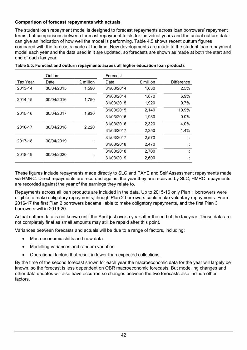
42

Comparison of forecast repayments with actuals The student loan repayment model is designed to forecast repayments across loan borrowers’ repayment terms, but comparisons between forecast repayment totals for individual years and the actual outturn data can give an indication of how well the model is performing. Table 4.5 shows recent outturn figures compared with the forecasts made at the time. New developments are made to the student loan repayment model each year and the data used in it are updated, so forecasts are shown as made at both the start and end of each tax year. Table 5.5: Forecast and outturn repayments across all higher education loan products

Outturn Forecast Tax Year Date £ million Date £ million Difference 2013-14 30/04/2015 1,590 31/03/2014 1,630 2.5%

2014-15 30/04/2016 1,750 31/03/2014

31/03/2015 1,870 1,920

6.9% 9.7%

2015-16 30/04/2017 1,930 31/03/2015

31/03/2016 2,140 1,930

10.9% 0.0%

2016-17 30/04/2018 2,220 31/03/2016

31/03/2017 2,320 2,250

4.0% 1.4%

2017-18 30/04/2019 : 31/03/2017

31/03/2018 2,570 2,470

: :

2018-19 30/04/2020 : 31/03/2018 2,700 : 31/03/2019 2,600 :

These figures include repayments made directly to SLC and PAYE and Self Assessment repayments made via HMRC. Direct repayments are recorded against the year they are received by SLC, HMRC repayments are recorded against the year of the earnings they relate to.

Repayments across all loan products are included in the data. Up to 2015-16 only Plan 1 borrowers were eligible to make obligatory repayments, though Plan 2 borrowers could make voluntary repayments. From 2016-17 the first Plan 2 borrowers became liable to make obligatory repayments, and the first Plan 3 borrowers will in 2019-20.

Actual outturn data is not known until the April just over a year after the end of the tax year. These data are not completely final as small amounts may still be repaid after this point.

Variances between forecasts and actuals will be due to a range of factors, including:

• Macroeconomic shifts and new data

• Modelling variances and random variation

• Operational factors that result in lower than expected collections. By the time of the second forecast shown for each year the macroeconomic data for the year will largely be known, so the forecast is less dependent on OBR macroeconomic forecasts. But modelling changes and other data updates will also have occurred so changes between the two forecasts also include other factors.

43

Advanced Learner Loans model Introduction Advanced Learner Loans (ALLs) are tuition fee loans to help those aged 19+ at the start of their course meet the up-front costs of regulated Further Education (FE) qualifications at Levels 3 (equivalent to 2 A levels) to Level 6 (equivalent to an undergraduate degree) in England. ALLs were introduced in 2013/14 to those aged 24+ and at levels 3-4 following a refocusing of the Adult Education Budget on adults requiring skills and learning to equip them for work, an apprenticeship or further learning.

Following a public consultation in 2014, the extension of ALLs in academic year 2016/17 to those aged 19-23 and to Levels 5-6 has been the programme’s most significant change.

The Resource Accounting and Budgeting (RAB) charge is the estimated cost to Government of borrowing to support the ALLs system. The purpose of the DfE ALLs model is to assist in valuing the existing ALLs loan book and to provide forecasts for budgeting purposes.

The RAB charge is an estimate and it is heavily dependent on assumptions around the future income of ALLs borrowers. At present, we have imperfect information about their repayment ability as ALLs are a new product and no significant number of ALLs borrowers have yet made a repayment. The first provisional repayment data was made available in summer 2018. The methodology, data sources and assumptions are presented in the section below.

Methodology The ALLs model is a micro-simulation model. The model creates thousands of simulated borrowers with a variety of characteristics. Each borrower is assigned a debt and their earnings are projected for each of the next 30 years. Then the repayment rules are applied to each borrower to estimate their repayments, individual loan balance and interest for each of the next 30 years. The assumptions used in the simulation model fall into five main sections below:

1. Borrowers’ characteristics and their loan details 2. Macroeconomic assumptions: Average Earnings Index (AEI) and Retail Price Index (RPI) 3. Loans policy assumptions 4. Annual income post learning: employment status, income and income distributions 4.1. Labour market status 4.2. Position on income distribution 4.3. Annual income in nominal terms 5. Life events 5.1. Mortality 5.2. Migration 5.3. Permanently unfit for work 5.4. Extending working lives.

1. Borrowers’ characteristics and their loan details Analysis of administrative Student Loans Company (SLC) data informs the input assumptions on the characteristics of borrowers in each academic year, the courses they study and the average loan size they take. The complete list of input parameters are:

• Total number of new borrowers;

• Proportion of borrowers on multiple courses;

• Course type: A levels, Access to HE, Level 3 Diploma, Level 4 Diploma, Level 3 Certificate, Level 4 Certificate and Level 5/Level 6 courses;

• Gender split of borrowers;

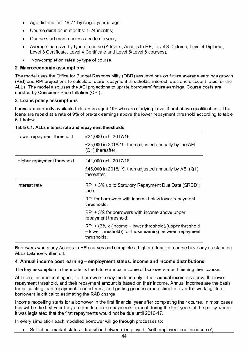
44

• Age distribution: 19-71 by single year of age;

• Course duration in months: 1-24 months;

• Course start month across academic year;

• Average loan size by type of course (A levels, Access to HE, Level 3 Diploma, Level 4 Diploma, Level 3 Certificate, Level 4 Certificate and Level 5/Level 6 courses).

• Non-completion rates by type of course. 2. Macroeconomic assumptions The model uses the Office for Budget Responsibility (OBR) assumptions on future average earnings growth (AEI) and RPI projections to calculate future repayment thresholds, interest rates and discount rates for the ALLs. The model also uses the AEI projections to uprate borrowers’ future earnings. Course costs are uprated by Consumer Price Inflation (CPI).

3. Loans policy assumptions Loans are currently available to learners aged 19+ who are studying Level 3 and above qualifications. The loans are repaid at a rate of 9% of pre-tax earnings above the lower repayment threshold according to table 6.1 below. Table 6.1: ALLs interest rate and repayment thresholds

Lower repayment threshold £21,000 until 2017/18;

£25,000 in 2018/19, then adjusted annually by the AEI (Q1) thereafter.

Higher repayment threshold £41,000 until 2017/18;

£45,000 in 2018/19, then adjusted annually by AEI (Q1) thereafter.

Interest rate RPI + 3% up to Statutory Repayment Due Date (SRDD); then

RPI for borrowers with income below lower repayment thresholds;

RPI + 3% for borrowers with income above upper repayment threshold;

RPI + (3% x (income – lower threshold)/(upper threshold – lower threshold)) for those earning between repayment thresholds.

Borrowers who study Access to HE courses and complete a higher education course have any outstanding ALLs balance written off.

4. Annual income post learning – employment status, income and income distributions The key assumption in the model is the future annual income of borrowers after finishing their course.

ALLs are income contingent, i.e. borrowers repay the loan only if their annual income is above the lower repayment threshold, and their repayment amount is based on their income. Annual incomes are the basis for calculating loan repayments and interest, and getting good income estimates over the working life of borrowers is critical to estimating the RAB charge.

Income modelling starts for a borrower in the first financial year after completing their course. In most cases this will be the first year they are due to make repayments, except during the first years of the policy where it was legislated that the first repayments would not be due until 2016-17.

In every simulation each modelled borrower will go through processes to:

• Set labour market status – transition between ‘employed’, ‘self-employed’ and ‘no income’;

45

• Assign position on income distribution – one of the 25 quantiles36 and

• Assign annual income based on their position in the income distributions. The process is summarised below in figure 6.1: Figure 6.1: Income modelling for ALL borrowers

4.1 Labour market status Labour market status in a given year is modelled using a discrete probability matrix which supports three possible outcomes: ‘no income’, ‘employed’ and ‘self-employed’. The matrix has different probabilities depending on the characteristics of the borrower:

• Course level: Level 4+ , Level 3

• Gender: male or female

• Age: single year of age

• Years since completed learning: one year, or more than one year

• Current labour market status: no income, employed or self-employed

• Current year income: one of 25 quantiles, or zero if not in work The data source for the analysis is 68 quarters of Labour Force Survey (LFS). The model uses two sets of labour market assumptions:

• Initial labour market status for those in the first full financial year after their SRDD.

• Probabilities of changing labour market status in all subsequent years. In the first year after SRDD the model has no knowledge about the working history of each borrower so borrowers are assigned a labour market status only in accordance with the overall employment rates for that age, gender and course level37. In all subsequent years each borrower has a probability of changing labour market status, this time taking into account their current labour market status and income quantile (if in work).

36 The income distribution is split into 25 equal quantile, so each quantile represents 4% of the income distribution. Quantile 1 = the lowest earning. The number of quantiles was determined by considering the greatest detail that the LFS could provide whilst still providing robust estimates. 37 Ideally, the data would be further restricted to learners that are one year post learning but there is insufficient data in the LFS to support this. The initial employment status is quickly eroded by the subsequent employment transition probabilities so has a fairly limited impact on the forecast.

46

Income data for the self-employed is not available from the LFS. This means that income based labour market changes from the employee population are used as a proxy, i.e. if an employed borrower at the bottom of the income distribution has a greater chance of becoming unemployed compared to someone at the top, then a self-employed borrower at the bottom of the income distribution also has a greater chance of becoming unemployed compared to someone at the top.

4.2 Position on income distribution After labour market status is established in the previous stage, the model assigns the borrower to a quantile on the income distribution. As with labour market status, the model assigns future income quantiles, using different probabilities depending on the characteristics of the borrower:

• Course Level: Level 4+, Level 3

• Gender: male or female

• Age: single year of age

• If in work: current income: one of 25 quantiles

• If out of work: previous income when last in work: one of 25 quantiles or zero if never previously modelled in work.

The LFS does not contain income for the self-employed so it is assumed that transitions across the income distribution for the self-employed occur with the same likelihood as for the employed.

The LFS data only has sufficient information to compare year on year income, it does not hold robust income information from previous employment spells further back in time. As a simplification it is assumed that a borrower returns to work at the same position on the income distribution as they were in their most recent modelled income spell, e.g. if they left work in quantile 10 then when they return to work they will return in quantile 10.

The LFS data suggests that typically those entering work are on lower incomes than the equivalent group leaving work. This would suggest a natural decay in position on the income distribution between jobs, i.e. that learners should return at a lower position on the income distribution. In practice this does not produce a good modelling solution as it creates a heavy penalty for being out of work in a single year and produces unexpected lifetime income paths inconsistent with the original simplified assumption.

4.3 Annual income in nominal terms The final step in modelling income is to convert an income quantile into actual income for a given financial year. This is achieved by matching the simulated income quantile to historic income quantile distributions. There are different distributions by:

• Course Level: Level 4+, Level 3

• Gender: male or female

• Age: single year of age

• Years since left learning bands: 1-3 years; 4-10 years; 11+ years Income distributions are constructed using 14 years of Annual Population Survey (APS). Income is inflated for future growth using OBR projections of average earnings growth for the entire working population. It is also assumed that average earnings growth is even across all quantiles.

5. Life events From the time a borrower takes out a loan there are additional events that need to be factored in to the modelling, such as mortality, migration, and repayments made directly to SLC. All are modelled at the individual level, but to varying levels of detail.

5.1 Mortality The Office for National Statistics (ONS) England & Wales population projections include assumptions on mortality rates by gender and single year of age up to 2084. These are used directly to estimate the chance of death for a borrower in any year post taking out a loan, with the key assumption that ALLs borrowers have the same mortality rates as the rest of the population.

47

It is likely there is some difference in mortality rates for this group compared to the whole of England & Wales, particularly as there is a known link between increased wealth and improved mortality. However, any difference will be minimal and the mortality rates for the working age population are generally very low, further reducing any possible impact.

5.2 Migration The migration assumptions are split into two components

• Probability of migrating out of the country (out-migrant rate)

• Length of spell out of the country: 3 years, 7 years or 20 years Out-migrant rates by gender and age are derived by combining Office for National Statistics (ONS) out-migrant estimates with population projections. These are used directly to provide each borrower with a probability of becoming an out-migrant each year.

Once an out-migrant is identified the model assigns a length of stay for the duration abroad. The length and probability of duration are estimated from International Passenger Survey (IPS) data between 1978 and 2012, over which time actual length of stay figures have been relatively stable.

5.3 Permanently unfit for work The model uses expected flows in to the Support Group of Employment Support Allowance (ESA) as a proxy for the number of people expected to become unfit for work each year. Once identified as unfit for work, a simulated borrower has their remaining loan amount written off.

The ESA Support Group is not a perfect measure of the unfit for work rate, as it is a State Benefit that needs to be actively claimed so is not received by everyone that is eligible. However it provides the closest match in definition to unfit for work which is sufficient for the relatively low number of people that will be affected.

5.4 Extending working lives State Pension Age (SPA) is due to rise to 67 for men and women by 2024. For women this represents an additional 7 years of work before they will receive their State retirement benefits compared to the observed population in the model data sources.

The model includes a timetable to assign each borrower a State Pension age, from which there is an assumption around what employment rates and income to use given to reflect that people are likely to work for longer. For example, a man with SPA of 65 has the employment rate of a 66 year old when aged 66, but a man with SPA of 66 has the employment rate of a 65 year old when aged 66. This assumes that for men, the employment rate and income of a 65 year old is held constant between the ages of 65 and the new State Pension age; for women the employment rate and income of a 60 year old is held constant between the ages of 60 and the new State Pension age.

The effects of retirement can be seen in LFS data from as early as age 50. However given the high uncertainty about how people will respond to the rises in State Pension age, and future employment in general, the model uses the simplified assumption.

Data quality There is a high level of uncertainty around the ALLs RAB and stock charges estimates. At present, we have imperfect information about ALLs borrowers’ repayment ability as ALLs are a new product and the first provisional set of repayment data was made available in summer 2018. When we receive the complete repayment data we will be able to compare this with the assumptions within the model and the resulting impact on the forecast.

Both administrative and survey data are used to inform the assumptions underpinning the ALLs model.

SLC administrative data are used to determine borrowers' characteristics and loan amounts. Historic SLC data should be broadly accurate. SLC quality guidelines are published on the following webpage: https://www.slc.co.uk/official-statistics/guide-to-our-statistics/compliance.aspx.

The Labour Force Survey (LFS) is used to determine employment and income state movements of ALLs borrowers and the Annual Population Survey (APS) for the income distributions. The LFS is a survey of the

48

employment circumstances of the UK population. It is the largest household survey in the UK and provides the official measures of employment and unemployment. The APS is a supplement to the LFS data. The APS is published quarterly and each dataset contains 12 months of data. The sample size for each dataset is approximately 170,000 households and 360,000 individuals.

The employment and income status assumptions are two of the most important assumptions within the model. We derive both of those from the LFS assuming that Further Education achievers in the LFS data are representative of ALLs borrowers.

The LFS data has various limitations and a key drawback is that only one year of earnings history is available. Also, the LFS does not capture self-assessment income, but does include a flag to identify employment status. The key assumptions arising from the data limitations are listed below:

• The model 'forgets' a borrower’s past history of employment statuses prior to the current year, since a one-step transition approach is used. This means that a learner who has been unemployed for 10 years has equal chance of employment as someone who has been unemployed for just one year.

• Transitions between employment states for the employed are used as a proxy for self-employed people. Self-employed people are assumed to have the same income distribution as employed learners.

• We assume that a borrower who has left the labour market will return to work at the same position on the income distribution as they were in their most recent employment spell.

Despite these limitations, the LFS is the only data source currently available that has a sufficiently large sample to allow analysis of income by age and type of qualifications and transitions in and out of employment. In the future it will be possible to use actual repayment data to improve these assumptions, as well as consider how data from the new Longitudinal Education Outcomes study could also be incorporated into the modelling.

The model is also dependent on the OBR macroeconomic forecasts that it uses to uprate earnings, calculate interest rates and repayment thresholds, and to discount future repayments to present values. Any significant changes to the economy from these forecasts could affect the repayments that will be made on the Advanced Learner Loans.

49

Uses of these statistics These forecasts show how much Government outlay on students loans is expected to be in future, how much is expected to be repaid and how the student loan book may grow in the future. The Department for Education uses these models for financial planning and in the development of student funding policies.

These forecasts are also used in the Department for Education’s annual accounts in the valuation of the student loan book. The stock and RAB charges are used to impair the face value of the loan books and the value of new loans being issued respectively, to reflect that the value of the future repayments that will be received in relation to these loans is less than the long term cost of Government borrowing that would be necessary to cover its outlay on student loans.

These models are used by the Office for Budget Responsibility as part of its estimates of public sector borrowing, including in its Economic and Fiscal Outlook that presents economic forecasts five years into the future and its Fiscal Sustainability Report that presents long term projections of UK public finances.

References Conlon, G., & Patrignani, P. (2011, June). BIS research paper number 45: The returns to higher education

qualifications. Retrieved from https://www.gov.uk/government/publications/higher-education-qualifications-returns-and-benefits

Nanton, A., & Rowling, J. (2017, September 25). Earnings and low pay: distributions and estimates from the Labour Force Survey. Retrieved from ONS: www.ons.gov.uk/employmentandlabourmarket/peopleinwork/earningsandworkinghours/articles/earningsandlowpay/distributionestimatesfromthelabourforcesurvey

Get in touch Media enquiries Press Office News Desk, Department for Education, Sanctuary Buildings, Great Smith Street, London SW1P 3BT.

Tel: 020 7783 8300

Other enquiries/feedback Peter Wrixon, Higher Education Analysis, Department for Education, Sanctuary Buildings, Great Smith Street, London, SW1P 3BT.

Email: he.modelling@education.gov.uk

© Crown copyright 2019

This publication (not including logos) is licensed under the terms of the Open Government Licence v3.0 except where otherwise stated. Where we have identified any third party copyright information you will need to obtain permission from the copyright holders concerned.

To view this licence: visit www.nationalarchives.gov.uk/doc/open-government-licence/version/3 email psi@nationalarchives.gsi.gov.uk write to Information Policy Team, The National Archives, Kew, London, TW9 4DU

About this publication: Enquiries: Peter Wrixon, Higher Education Analysis, Department for Education, Sanctuary Buildings, Great Smith Street, London, SW1P 3BT. Email: he.modelling@education.gov.uk https://www.gov.uk/government/statistics/student-loan-forecasts-england-2017-to-2018

Reference: Student loan forecasts, England: 2018-19: Quality and methodology information

Follow us on Twitter: @educationgovuk

Like us on Facebook: facebook.com/educationgovuk