i

Copy No.

Guide for Mechanistic-Empirical Design OF NEW AND REHABILITATED PAVEMENT

STRUCTURES

FINAL DOCUMENT

APPENDIX RR: FINITE ELEMENT PROCEDURES FOR FLEXIBLE

PAVEMENT ANALYSIS

NCHRP

Prepared for National Cooperative Highway Research Program

Transportation Research Board National Research Council

Submitted by ARA, Inc., ERES Division

505 West University Avenue Champaign, Illinois 61820

February 2004

ii

Foreword The finite element code that is used for the non-linear assessment of flexible (AC) pavement systems in the analysis and design methodology of the Design Guide, and referred to in this Appendix, is a modified and enhanced version of the DSC2D finite element code originally developed by Dr. C. S. Desai at the University of Arizona, Tucson. Significant additions, modifications and enhancements were implemented by Dr. Schwartz and his research team in order to fully implement the DSC2D code properly into the 2002 Design Guide approach. Some of the major enhancements, completed by the University of Maryland research team, dealt with the following issues: • Formulation of the final non-linear Mr (resilient modulus) implementation scheme for

all unbound base, subbase and subgrade layers characterized by the 3 parameter ki non-linear model function selected for use in the Design Guide analysis methodology.

• Development of an enhanced tension cutoff model and associated convergence routines.

• Development of practical user guidelines, including details of incorporating infinite elements at the boundaries of the mesh, as well as sensitivity studies to determine the appropriate locations for the infinite elements within the mesh.

• Restructuring the DSC2D model to efficiently predict pavement response values in the continuous, multi-seasonal analysis used in the cumulative incremental damage approach employed in both the linear or non-linear pavement analysis approaches of the 2002 Design Guide.

• Development of both pre and post processors for the DSC2D to generate finite element pavement models from the main program user interface and to extract salient pavement damages and distress quantities from the stresses and strains computed by the finite element program.

• Finally, the development of the detailed user documentation for the code formulation and implementation as presented in this Appendix.

Note that general two and three dimensional disturbed state concept DSC codes, with many additional features, such as a wide selection of material models (elastic, plastic, HISS, creep, disturbance (damage), static, dynamic and repetitive loading, coupled fluid effects and thermal loading) have been developed by C.S.Desai and are available. These programs have been validated for a wide range of engineering problems, including pavement systems. For further information, one can visit the web site: dscfe.com; write to DSC, P.O. Box 65587, Tucson, Arizona 85728 or e-mail: support@dscfe.com Acknowledgements The research team for NCHRP Project 1-37A: Development of the 2002 Guide for the Design of New and Rehabilitated Pavement Structures consisted of Applied Research Associates, Inc. (ERES Division) as the prime contractor with Arizona State University (ASU) and Fugro-BRE, Inc. as subcontractors. University of Maryland and Advanced Asphalt Technologies, LLC served as subcontractors to the Arizona State University along with several independent consultants.

iii

Research into this subject area was conducted in ASU under the guidance of Dr. M. W. Witczak. Dr Witczak was assisted by Dr. C. W. Schwartz and Mr. Y.Y. Feng of the University of Maryland. Other contributors were Dr. Jacob Uzan of Technion University (Israel) and Dr. Waseem Mirza of ASU. The pioneering work of Dr. C. S. Desai at the University of Arizona in developing the original version of the DSC2D finite element code is gratefully acknowledged.

iv

TABLE OF CONTENTS TABLE OF CONTENTS................................................................................................... iv LIST OF FIGURES ........................................................................................................... vi LIST OF TABLES.............................................................................................................. x 1. INTRODUCTION ...................................................................................................... 1

1.1 Objectives of Pavement Response Models ............................................................. 1 1.2 Accuracy of Pavement Performance Predictions.................................................... 4

1.2.1 Sources of Error in Performance Predictions..................................................... 4 1.2.2 Validation of Pavement Response Models ........................................................ 6

1.3 Selection of Analysis Method................................................................................. 10 1.3.1 Material Behavior ............................................................................................ 10 1.3.2 Problem Dimensionality .................................................................................. 13 1.3.3 Computational Practicality............................................................................... 14 1.3.4 Implementation Considerations ....................................................................... 33

1.3 Summary of Finite Element Advantages and Disadvantages ................................. 34 2. SELECTION OF FINITE ELEMENT PROGRAM..................................................... 37

2.1 Key Issues ............................................................................................................... 37 2.1.1 Efficiency Issues .............................................................................................. 37 2.1.2 Operational Issues............................................................................................ 39

2.2 Key Features Of Candidate Programs..................................................................... 40 2.3 Final Selection ........................................................................................................ 42

3. ORGANIZATION OF THE FINITE ELEMENT PROGRAMS................................. 45 4. DSC2D FINITE ELEMENT PROGRAM.................................................................... 50

4.1 Basic Formulation................................................................................................... 50 4.2 Nonlinear Resilient Modulus Model....................................................................... 53

4.2.1 Finite Element Implementation........................................................................ 57 4.2.2 Importance of Nonlinear Behavior .................................................................. 64 4.2.3 Nonlinear Superposition .................................................................................. 89

4.3 Infinite Boundary Element.................................................................................... 107 4.3.1 Finite Element Formulation ........................................................................... 107 4.3.2 Guidelines for Infinite Boundary Element Location ..................................... 115

5. PRE-DSC PREPROCESSOR PROGRAM ................................................................ 127 6. POST-DSC POSTPROCESSING PROGRAM.......................................................... 130 7. PROGRAM INPUT/OUTPUT FILES ....................................................................... 131

7.1 Overview............................................................................................................... 131 7.1.1 PRE-DSC Pre-Processor Program ................................................................. 131 7.1.2 DSC2D Finite Element Program ................................................................... 132 7.1.3 POST-DSC Post-Processor Program ............................................................. 132

7.2 PRE-DSC Input/Output Files................................................................................ 133 LAYERS.CSV ........................................................................................................ 133 LAYERS.INI .......................................................................................................... 135 LOADLEVELS.CSV.............................................................................................. 137 PREPOST.DAT ...................................................................................................... 138 PROJECT_TANDEMAXLEOUTPUT.CSV ......................................................... 140 PROJECT_TRIDEMAXLEOUTPUT.CSV ........................................................... 140

v

PROJECT_QUADAXLEOUTPUT.CSV............................................................... 140 7.3 DSC2D Input/Output Files ................................................................................... 142

DSC.IN.................................................................................................................... 143 Emmmm-nn.OUT ................................................................................................... 154

7.4 POST-DSC Input/Output Files ............................................................................. 155 FATIGUE.OUT ...................................................................................................... 155 PERMDEF.OUT..................................................................................................... 156

8. PROGRAMMER DOCUMENTATION FOR FINITE ELEMENT PROGRAMS... 157 8.1 Subroutine Calls for DSC2D ................................................................................ 158

8.1.1 Linear Solution............................................................................................... 159 8.1.2 Nonlinear Solution......................................................................................... 161

8.2 COMMON Variables in DSC2D.......................................................................... 163 8.3 Array Pointers in DSC2D ..................................................................................... 166

9. REFERENCES ........................................................................................................... 168 10. ALTERNATIVE FORMULATION FOR NONLINEAR MR ................................. 174

vi

LIST OF FIGURES

Figure 1. Conceptual depiction of relative uncertainties of components in pavement performance prediction system. .................................................................................. 6

Figure 2. Sand test pit for comparison of measured vs. predicted stresses. (Ullidtz, Askegaard, and Sjolin, 1996)...................................................................................... 8

Figure 3. Comparison of measured vs. predicted stresses for sand test pit. (Ullidtz, Askegaard, and Sjolin, 1996)...................................................................................... 8

Figure 4. Comparisons between backcalculated and measured asphalt tension strains at MnRoad (Dai et al., 1987). ......................................................................................... 9

Figure 5. Comparisons between predicted and measured subgrade stresses at the Danish test road (Ertman, Larsen, and Ullidtz, 1987)............................................................. 9

Figure 6. Theoretical vs. measured pavement stresses and strains (Ullidtz, 1998). [Note: Low values (<50) are stresses on the subgrade in kPa; intermediate values (50-400) are asphalt tensile strains in µε; higher values (100-600) are subgrade compressive strains in µε; (P. Ullidtz, personal communication).] ............................................... 10

Figure 7. Nonlinear material behavior. ............................................................................ 11 Figure 8. Example of influence of nonlinear unbound material on predicted surface

deflections (Chen et al., 1995). ................................................................................. 12 Figure 9. Comparison of measured subgrade vertical strain against predictions from

linearly elastic pavement response models (Ullidtz, 1998). ..................................... 13 Figure 10. Computation times for KENLAYER .............................................................. 19 Figure 11. Computation times for JULEA........................................................................ 20 Figure 12. Coarse refinement mesh (396 elements) ......................................................... 23 Figure 13. Medium refinement mesh (1584 elements) ..................................................... 24 Figure 14. Fine refinement mesh (3564 elements) ........................................................... 25 Figure 15. Surface displacements computed at different mesh refinements. ................... 26 Figure 16. Vertical stresses along centerline at different mesh refinements. ................... 26 Figure 17. Horizontal stresses along centerline at different mesh refinements. ............... 27 Figure 18. Comparison of finite element execution times. ............................................... 27 Figure 19. Medium refinement mesh with distant infinite boundary elements. ............... 29 Figure 20. Medium refinement mesh with close infinite boundary elements................... 30 Figure 21. Finite element solution times using infinite boundary elements. .................... 31 Figure 22. Overall program flow. ..................................................................................... 46 Figure 23. Data flow from the 2002 Design Guide user interface program. .................... 47 Figure 24. Data flow for PRE-DSC pre-processor program............................................. 47 Figure 25. Data flow for DSC2D finite element program. ............................................... 48 Figure 26. Data flow for POST-DSC post-processor program......................................... 49 Figure 27. Data flow to 2002 Design Guide user interface program................................ 49 Figure 28. Conceptual depiction of finite element model................................................. 52 Figure 29. Schematic of incremental iterative nonlinear solution technique.................... 52 Figure 30. Definition of resilient modulus as a chord modulus........................................ 56 Figure 31. Normalized stress, tangent modulus, and secant modulus vs. strain (k1=1000;

k2=0.25, 0.5, 0.75; k3=-0.3; σc=0)............................................................................. 62

vii

Figure 32. Normalized stress, tangent modulus, and secant modulus vs. strain (k1=1000; k2=0.5; k3=-0.1, -0.3, -0.5; σc=0) .............................................................................. 63

Figure 33. 3D Finite element mesh for nonlinear exploratory analyses. .......................... 65 Figure 34. Cross section of finite element mesh showing calculation locations. ............. 66 Figure 35. Variation of base layer MR with depth for single wheel loading. ................... 67 Figure 36. Effect of base layer nonlinearity on surface deflection beneath tire centerline.

................................................................................................................................... 67 Figure 37. Effect of base layer nonlinearity on horizontal tensile strain at bottom of

asphalt layer beneath tire centerline.......................................................................... 68 Figure 38. Effect of base layer nonlinearity on compressive strains at the midthickness of

the base layer and at the top of the subgrade beneath tire centerline........................ 68 Figure 39. Traffic structures considered for nonlinear analyses....................................... 71 Figure 40. Distribution of base layer modulus values for stress stiffening conditions,

k2=0.5, k3=0. ............................................................................................................. 72 Figure 41. Distribution of base layer modulus values for stress softening conditions, k2=0,

k3= -0.75.................................................................................................................... 73 Figure 42. Distribution of base layer modulus values for mixed stress stiffening/stress

softening conditions, k2=0.5, k3= -0.75 .................................................................... 74 Figure 43. Type 1 errors: High traffic structure, stress stiffening conditions (k2>0, k3=0).

(a) AC tensile strains. (b) Subgrade compressive strains. ........................................ 81 Figure 44. Type 2 errors: High traffic structure, stress stiffening conditions (k2>0, k3=0).

(a) AC tensile strains. (b) Subgrade compressive strains. ........................................ 82 Figure 45. Type 1 errors: High traffic structure, stress softening conditions (k2=0, k3<0).

(a) AC tensile strains. (b) Subgrade compressive strains. ........................................ 83 Figure 46. Type 2 errors: High traffic structure, stress softening conditions (k2=0, k3<0).

(a) AC tensile strains. (b) Subgrade compressive strains. ........................................ 84 Figure 47. Type 1 errors: Low traffic structure, stress stiffening conditions (k2>0, k3=0).

(a) AC tensile strains. (b) Subgrade compressive strains. ........................................ 85 Figure 48. Type 2 errors: Low traffic structure, stress stiffening conditions (k2>0, k3=0).

(a) AC tensile strains. (b) Subgrade compressive strains. ........................................ 86 Figure 49 Type 1 errors: Low traffic structure, stress softening conditions (k2=0, k3<0).

(a) AC tensile strains. (b) Subgrade compressive strains. ........................................ 87 Figure 50. Type 2 errors: Low traffic structure, stress softening conditions (k2=0, k3<0).

(a) AC tensile strains. (b) Subgrade compressive strains. ........................................ 88 Figure 51. 3D finite element mesh for nonlinear superposition study.............................. 98 Figure 52. Cross section of finite element mesh showing calculation locations. ............. 98 Figure 53. Degree of stress dependence considered in analyses (initial confining pressure

= 6.9 kPa). ................................................................................................................. 99 Figure 54. Variation of base layer MR with depth for single wheel nonlinear solutions.100 Figure 55. Variation of vertical stress with depth beneath a wheel for k2=0.8. (Notation:

Dual NL = Dual Wheel Nonlinear solution; S+S NL = Superimposed Single Wheel Nonlinear solution; S+S L = Superimposed Single Wheel Linear solution. See Figure 52 for stress/strain computation locations.)................................................. 101

Figure 56. Variation of horizontal stress with depth beneath a wheel for k2=0.8. (See Figure 55 caption for notation) ............................................................................... 101

viii

Figure 57. Variation of vertical strain with depth beneath a wheel for k2=0.8. (See Figure 55 caption for notation)........................................................................................... 102

Figure 58. Variation of horizontal strain with depth beneath a wheel for k2=0.8. (See Figure 55 caption for notation) ............................................................................... 102

Figure 59. Variation of vertical displacement with depth beneath a wheel for k2=0.8. (See Figure 55 caption for notation) ............................................................................... 103

Figure 60. Surface deflection beneath a wheel for k2=0.8. (See Figure 55 caption for notation) .................................................................................................................. 103

Figure 61. Errors in AC tensile stress determination. (Notation: Nonlinear = Superimposed Single Wheel Nonlinear Solutions; Linear = Superimposed Single Wheel Linear Solution; k2 = bulk stress exponent in Eq.(8)) ................................. 104

Figure 62. Errors in subgrade compressive stress determination (See Figure 61 for notation). ................................................................................................................. 104

Figure 63. Errors in AC tensile strain determination (See Figure 61 for notation). ...... 105 Figure 64. Errors in subgrade compressive strain determination (See Figure 61 for

notation). ................................................................................................................. 105 Figure 65. Errors in surface deflection determination (See Figure 61 for notation)..... 106 Figure 66. Effect of AC layer stiffness on errors for pavement response variables. ...... 106 Figure 67. A semi-infinite domain: soil deformations accompanying excavation. (a)

Conventional treatment. (b) Infinite element treatment. (from Zienkiewicz and Taylor, 1989)........................................................................................................... 110

Figure 68. Infinite line and element map. Linear η interpolation. (from Zienkiewicz and Taylor, 1989)........................................................................................................... 111

Figure 69. Infinite element map. Quadratic η interpolation. (from Zienkiewicz and Taylor, 1989)........................................................................................................... 112

Figure 70. Infinite boundary elements for point load on an elastic half-space (from Hibbitt, Karlsson, and Sorensen, 1998). ................................................................. 113

Figure 71. Infinite boundary elements for strip footing on infinitely extending layer of soil (from Hibbitt, Karlsson, and Sorensen, 1998). ................................................ 113

Figure 72. Infinite boundary elements for quarter plate with square hole (from Hibbitt, Karlsson, and Sorensen, 1998)................................................................................ 114

Figure 73. Examples of an acceptable and unacceptable infinite element (from Hibbitt, Karlsson, and Sorensen, 1998)................................................................................ 114

Figure 74. Mesh schematic for infinite boundary element study.................................... 118 Figure 75. Surface deflection vs. infinite boundary element location: (a) Soft AC,

EAC=500 MPa; (b) Stiff AC, EAC=12,500 MPa. ..................................................... 119 Figure 76. AC tensile stress vs. infinite boundary element location: s (a) Soft AC,

EAC=500 MPa; (b) Stiff AC, EAC=12,500 MPa. ..................................................... 120 Figure 77. AC tensile strain vs. infinite boundary element location: (a) Soft AC,

EAC=500 MPa; (b) Stiff AC, EAC=12,500 MPa. ..................................................... 121 Figure 78. Vertical compressive stress at center of base layer vs. infinite boundary

element location: (a) Soft AC, EAC=500 MPa; (b) Stiff AC, EAC=12,500 MPa.... 122 Figure 79. Vertical compressive strain at center of base layer vs. infinite boundary

element location: (a) Soft AC, EAC=500 MPa; (b) Stiff AC, EAC=12,500 MPa.... 123 Figure 80. Vertical compressive stress at top of subgrade vs. infinite boundary element

location: (a) Soft AC, EAC=500 MPa; (b) Stiff AC, EAC=12,500 MPa. ................ 124

ix

Figure 81. Vertical compressive strain at top of subgrade vs. infinite boundary element location: (a) Soft AC, EAC=500 MPa; (b) Stiff AC, EAC=12,500 MPa. ................ 125

Figure 82. Control parameters for mesh generation by PRE-DSC................................. 129 Figure 83. Plan view of calculation points for general traffic loading. .......................... 130 Figure 84. Mesh conventions.......................................................................................... 152 Figure 85. Local node numbering conventions for elements.......................................... 153 Figure 86. Accuracy of alternative nonlinear MR formulation--monotonic axial loading

case. [σc = 0, k1 = 1000, k2 = 0.7, k3 = -5, k6 = -33.8, k7 = 1] .................................. 176 Figure 87. Accuracy of alternative nonlinear MR formulation--monotonic axial loading

case. [σc = 0, k1 = 1000, k2 = 0.9, k3 = -0.1, k6 = -33.8, k7 = 1] ............................... 176

x

LIST OF TABLES

Table 1. New construction and rehabilitation scenarios for flexible pavements. ............... 4 Table 2. Variability among key pavement response parameters as computed using various

linearly elastic static analysis procedures; C.O.V = coefficient of variation. (Chen et al., 1995) ..................................................................................................................... 7

Table 3. Differences between linear and nonlinear analyses as reported by Chen et al. (1995)........................................................................................................................ 12

Table 4. Computational times for various analysis methods as reported in the literature.16 Table 5. Finite element mesh sizes for infinite boundary element study.......................... 31 Table 6. Timing comparisons between DSC2D and ABAQUS. ...................................... 33 Table 7. Comparison of technical features of the programs. ............................................ 41 Table 8. Evaluation of candidate programs against key issues......................................... 44 Table 9. Soil types tested by Andrei (2001). .................................................................... 56 Table 10. Typical values for k1, k2, and k3 in the simplified form of Equation (8) with

k6=0 and k7=1 (Andrei, 2001)................................................................................... 57 Table 11. Material properties for nonlinear exploratory analyses .................................... 66 Table 12. Material properties for nonlinear analysis parametric study . (High traffic

pavement structure)................................................................................................... 77 Table 13. Material properties for nonlinear analysis parametric study. (Low traffic

pavement structure)................................................................................................... 78 Table 14. Typical values for K1 and K2 (Huang, 1993).................................................... 97 Table 15. Material properties for nonlinear superposition analyses ................................. 97 Table 16. Material properties for infinite boundary element parametric study .............. 117 Table 17. Vertical stress attenuation vs. distance for Boussinesq circular load solution.

................................................................................................................................. 126 Table 18. Material property values for different constitutive models. (Note: Empty cells

imply that the property is not used in the constitutive model; enter a value of 0 in this case.)................................................................................................................. 151

RR-1

APPENDIX RR:

FINITE ELEMENT PROCEDURES FOR FLEXIBLE PAVEMENT ANALYSIS

1. INTRODUCTION

Two analytical approaches have been adopted for the flexible pavement response models in the 2002 Design Guide. For the most general case of nonlinear unbound material behavior (i.e., highest hierarchical level for flexible pavement material characterization), the two-dimensional nonlinear finite element analysis is used to predict the stresses, strains, and displacements in the pavement system under traffic loading for given environmental conditions. The purpose of this appendix is to describe the rationale behind adoption of nonlinear finite element techniques for the pavement response model and the criteria governing the selection of the DSC2D finite element computer program. This appendix also provides technical and user documentation for the finite element programs as implemented in the 2002 Design Guide. For the case of purely linear material behavior, the JULEA multilayer elastic theory (MLET) program is used for the pavement response model. A description of MLET theory and documentation for JULEA are provided in a separate appendix.

1.1 Objectives of Pavement Response Models

The purpose of the flexible pavement response model is to determine the structural response of the pavement system due to traffic loads and environmental influences. Environmental influences may be direct (e.g., strains due to thermal expansion and/or contraction) or indirect via effects on material properties (e.g., changes in stiffness due to temperature and/or moisture effects). Inputs to the flexible pavement response model include:

1. Pavement geometry a. Layer thicknesses b. Discontinuities (e.g., cracks, layer separations)

2. Environment

a. Temperature vs. depth for each season b. Moisture vs. depth for each season

3. Material properties (adjusted for environmental and other effects, as necessary) a. Elastic properties b. Nonlinear properties (where appropriate)

4. Traffic

RR-2

a. Load spectrum—i.e., frequencies of vehicle types and weights within each vehicle type

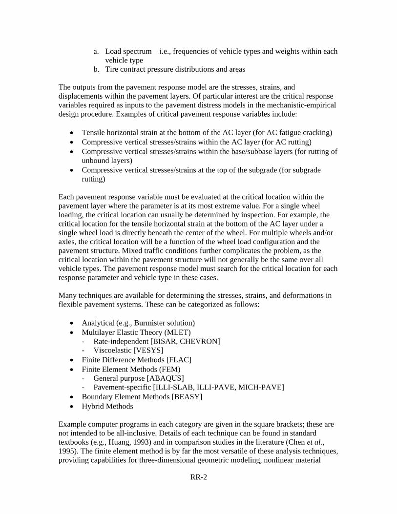
b. Tire contract pressure distributions and areas The outputs from the pavement response model are the stresses, strains, and displacements within the pavement layers. Of particular interest are the critical response variables required as inputs to the pavement distress models in the mechanistic-empirical design procedure. Examples of critical pavement response variables include:

• Tensile horizontal strain at the bottom of the AC layer (for AC fatigue cracking) • Compressive vertical stresses/strains within the AC layer (for AC rutting) • Compressive vertical stresses/strains within the base/subbase layers (for rutting of

unbound layers) • Compressive vertical stresses/strains at the top of the subgrade (for subgrade

rutting) Each pavement response variable must be evaluated at the critical location within the pavement layer where the parameter is at its most extreme value. For a single wheel loading, the critical location can usually be determined by inspection. For example, the critical location for the tensile horizontal strain at the bottom of the AC layer under a single wheel load is directly beneath the center of the wheel. For multiple wheels and/or axles, the critical location will be a function of the wheel load configuration and the pavement structure. Mixed traffic conditions further complicates the problem, as the critical location within the pavement structure will not generally be the same over all vehicle types. The pavement response model must search for the critical location for each response parameter and vehicle type in these cases. Many techniques are available for determining the stresses, strains, and deformations in flexible pavement systems. These can be categorized as follows:

• Analytical (e.g., Burmister solution) • Multilayer Elastic Theory (MLET)

- Rate-independent [BISAR, CHEVRON] - Viscoelastic [VESYS]

• Finite Difference Methods [FLAC] • Finite Element Methods (FEM)

- General purpose [ABAQUS] - Pavement-specific [ILLI-SLAB, ILLI-PAVE, MICH-PAVE]

• Boundary Element Methods [BEASY] • Hybrid Methods

Example computer programs in each category are given in the square brackets; these are not intended to be all-inclusive. Details of each technique can be found in standard textbooks (e.g., Huang, 1993) and in comparison studies in the literature (Chen et al., 1995). The finite element method is by far the most versatile of these analysis techniques, providing capabilities for three-dimensional geometric modeling, nonlinear material

RR-3

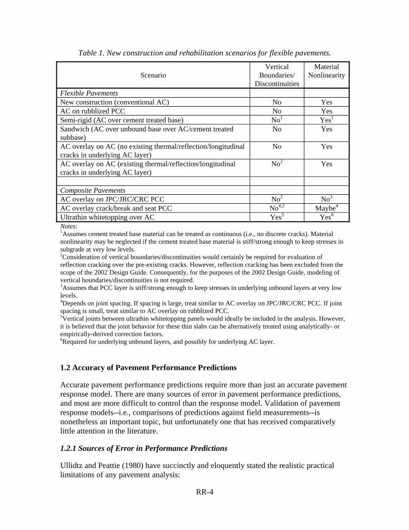
characterization, large strains/deformations, dynamic analysis, and other sophisticated features. Note that a general pavement response model is capable of computing much more than the critical pavement response quantities. However, the primary objective of the mechanistic-empirical design methodology in the 2002 Design Guide is to design pavements based on predicted pavement performance. The critical pavement response quantities required by the pavement distress models are, therefore, the primary outputs of the pavement response model. All other outputs are secondary and supplementary. The pavement response model must be capable of analyzing in a sufficiently realistic manner all of the flexible pavement new construction and rehabilitation scenarios considered in the 2002 Design Guide. In addition, the flexible pavement response model may also be used to analyze certain composite pavement scenarios. Table 1 summarizes the general set of new construction and rehabilitation scenarios for flexible and composite pavements considered in the 2002 Design Guide, along with evaluations of the importance of discontinuities (joints, cracks) and material nonlinearity in each scenario. It is important to note that reflection cracking was explicitly removed from the project team’s work scope by the project panel. Because of this, analysis complexities caused by the underlying vertical cracks (discontinuities) do not need to be considered in the flexible pavement response model. For the design approach proposed for the 2002 Design Guide, the core analysis capabilities required in the flexible pavement response model are as follows:

• Linear material model for AC, other bound, and unbound layers (lowest hierarchical level for unbound material characterization)

• Stress-dependent material model (nonlinear resilient modulus with tension cut-off) for unbound materials (highest hierarchical level for unbound material characterization)

• Quasi-static monotonically increasing loading from single or multiple wheel configurations

• Fully bonded, full slip, and intermediate interface conditions between layers

RR-4

Table 1. New construction and rehabilitation scenarios for flexible pavements.

Scenario

Vertical Boundaries/

Discontinuities

Material Nonlinearity

Flexible Pavements New construction (conventional AC) No Yes AC on rubblized PCC No Yes Semi-rigid (AC over cement treated base) No1 Yes1 Sandwich (AC over unbound base over AC/cement treated subbase)

No Yes

AC overlay on AC (no existing thermal/reflection/longitudinal cracks in underlying AC layer)

No Yes

AC overlay on AC (existing thermal/reflection/longitudinal cracks in underlying AC layer)

No2 Yes

Composite Pavements AC overlay on JPC/JRC/CRC PCC No2 No3 AC overlay crack/break and seat PCC No4,2 Maybe4

Ultrathin whitetopping over AC Yes5 Yes6

Notes: 1Assumes cement treated base material can be treated as continuous (i.e., no discrete cracks). Material nonlinearity may be neglected if the cement treated base material is stiff/strong enough to keep stresses in subgrade at very low levels. 2Consideration of vertical boundaries/discontinuities would certainly be required for evaluation of reflection cracking over the pre-existing cracks. However, reflection cracking has been excluded from the scope of the 2002 Design Guide. Consequently, for the purposes of the 2002 Design Guide, modeling of vertical boundaries/discontinuities is not required. 3Assumes that PCC layer is stiff/strong enough to keep stresses in underlying unbound layers at very low levels. 4Depends on joint spacing. If spacing is large, treat similar to AC overlay on JPC/JRC/CRC PCC. If joint spacing is small, treat similar to AC overlay on rubblized PCC. 5Vertical joints between ultrathin whitetopping panels would ideally be included in the analysis. However, it is believed that the joint behavior for these thin slabs can be alternatively treated using analytically- or empirically-derived correction factors. 6Required for underlying unbound layers, and possibly for underlying AC layer.

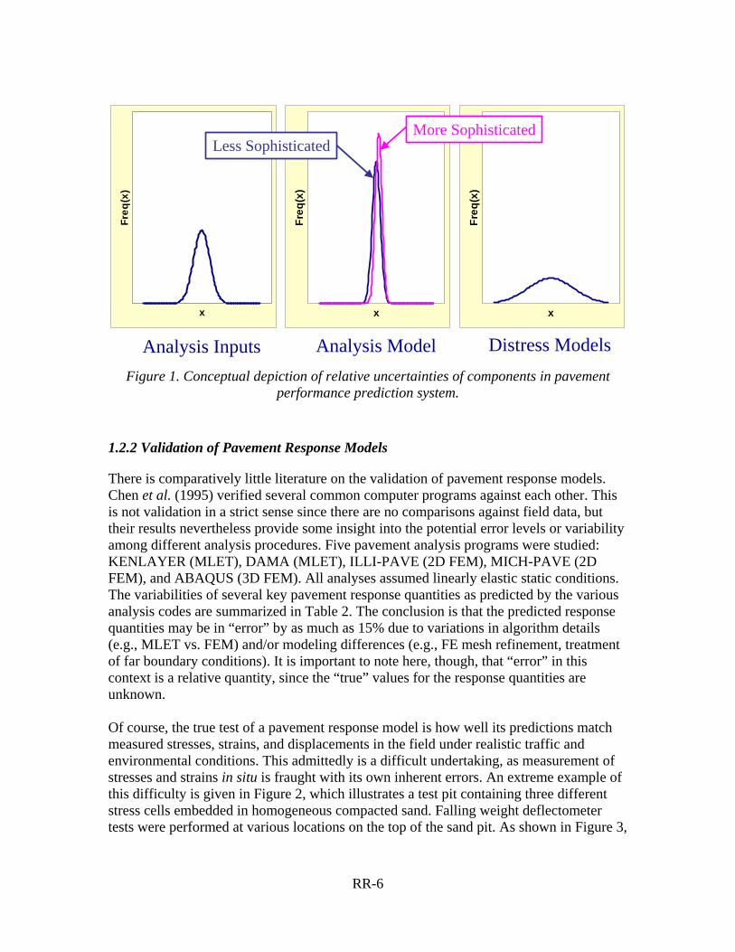
1.2 Accuracy of Pavement Performance Predictions

Accurate pavement performance predictions require more than just an accurate pavement response model. There are many sources of error in pavement performance predictions, and most are more difficult to control than the response model. Validation of pavement response models--i.e., comparisons of predictions against field measurements--is nonetheless an important topic, but unfortunately one that has received comparatively little attention in the literature.

1.2.1 Sources of Error in Performance Predictions

Ullidtz and Peattie (1980) have succinctly and eloquently stated the realistic practical limitations of any pavement analysis:

RR-5

“The … results obtained [from the analysis] may deviate from the exact values. These deviations, however, should be considered in relation both to the simplifications made in the analysis and to the variations of materials and structures with space and time. Real pavements are not infinite in horizontal extent, and subgrade materials are not semi-infinite spaces. The materials are nonlinear, elastic, anisotropic, and inhomogeneous, and some are particulate; viscous and plastic deformations occur in addition to the elastic deformations; loadings are not usually circular or uniformly distributed, and so on. To these differences between real and theoretical structures should be added the very large variations in layer thicknesses and elastic parameters from point to point, and during the life of a pavement structure. Moreover, it is a fact that precise information on the elastic parameters of granular materials and subgrades is in most cases very limited. For most practical purposes, therefore, the accuracy of the…methods should be quite sufficient.”

Ullidtz and Peattie made these observations twenty years ago in the context of their Equivalent Thickness approximate method and linear elasticity, but the general thrust of the comments applies equally well today to even the most sophisticated pavement analysis techniques. The design methodology in the 2002 Design Guide is based on mechanistic-empirical predictions of pavement performance. There are many components and subsystems involved in making these predictions: inputs such as traffic loading, environmental conditions, and material properties; the pavement response model; and the empirical distress prediction models. Each of these components has an inherent inaccuracy or uncertainty, as shown conceptually in Figure 1. In general, the level of inaccuracy or uncertainty in the material inputs and, especially, the distress prediction models will be far greater than that of the pavement response calculations. Within this context, for example, the additional modest differences between a 2D vs. 3D pavement response calculation may be insignificant in practical terms. This point was already recognized during earlier attempts to develop a mechanistic-empirical pavement design procedure (Thompson, 1990):

“The development of more sophisticated/complex/realistic structural models does not necessarily insure an ‘improved’ pavement design procedure. In fact, the structural model is frequently the ‘most advanced’ component! INPUTS and TRANSFER FUNCTIONS are generally the components lacking precision.”

A key strength of mechanics-based pavement response models such as those incorporated in the 2002 Design Guide, however, is that they enable the engineer to make a rational assessment the relative impacts of the various inputs and transfer functions—and their associated variations and uncertainties—on the pavement structural response.

RR-6

xFr

eq(x

)x

Freq

(x)

x

Freq

(x)

Analysis Inputs Analysis Model Distress Models

More SophisticatedLess Sophisticated

Figure 1. Conceptual depiction of relative uncertainties of components in pavement

performance prediction system.

1.2.2 Validation of Pavement Response Models

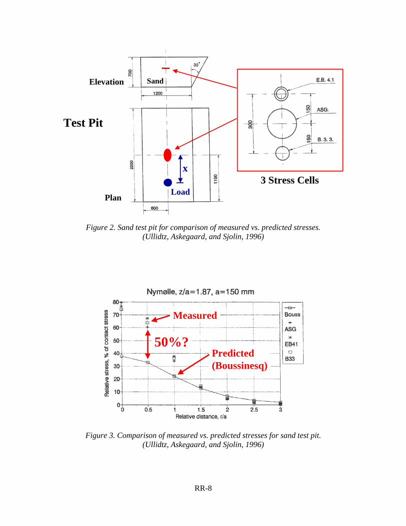
There is comparatively little literature on the validation of pavement response models. Chen et al. (1995) verified several common computer programs against each other. This is not validation in a strict sense since there are no comparisons against field data, but their results nevertheless provide some insight into the potential error levels or variability among different analysis procedures. Five pavement analysis programs were studied: KENLAYER (MLET), DAMA (MLET), ILLI-PAVE (2D FEM), MICH-PAVE (2D FEM), and ABAQUS (3D FEM). All analyses assumed linearly elastic static conditions. The variabilities of several key pavement response quantities as predicted by the various analysis codes are summarized in Table 2. The conclusion is that the predicted response quantities may be in “error” by as much as 15% due to variations in algorithm details (e.g., MLET vs. FEM) and/or modeling differences (e.g., FE mesh refinement, treatment of far boundary conditions). It is important to note here, though, that “error” in this context is a relative quantity, since the “true” values for the response quantities are unknown. Of course, the true test of a pavement response model is how well its predictions match measured stresses, strains, and displacements in the field under realistic traffic and environmental conditions. This admittedly is a difficult undertaking, as measurement of stresses and strains in situ is fraught with its own inherent errors. An extreme example of this difficulty is given in Figure 2, which illustrates a test pit containing three different stress cells embedded in homogeneous compacted sand. Falling weight deflectometer tests were performed at various locations on the top of the sand pit. As shown in Figure 3,

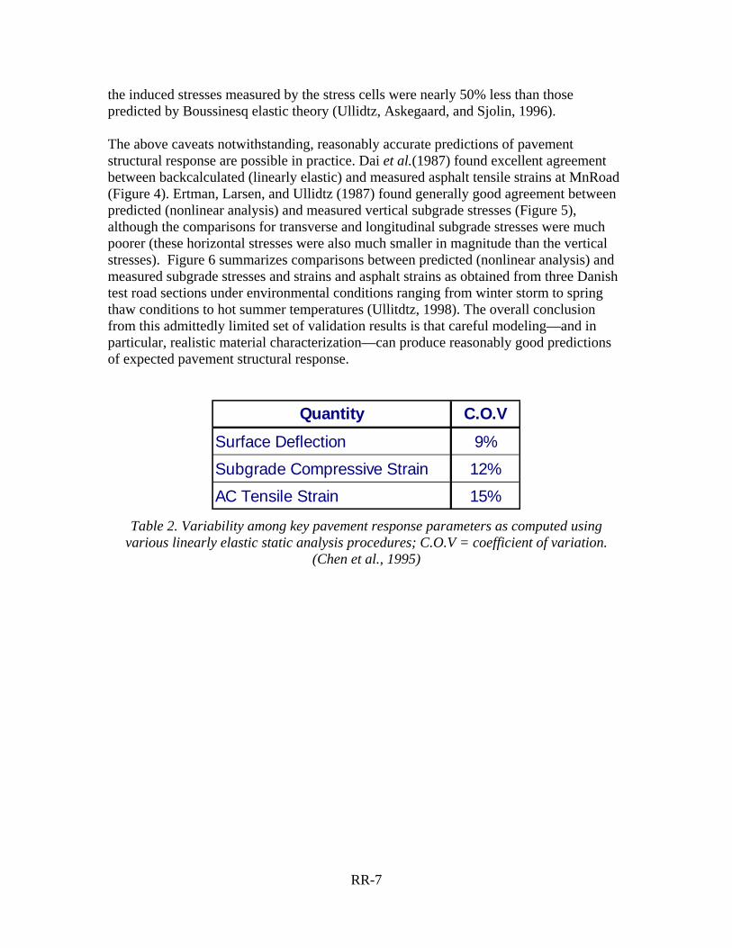
RR-7

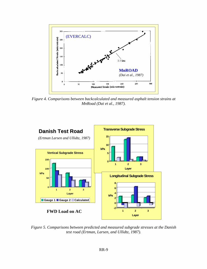
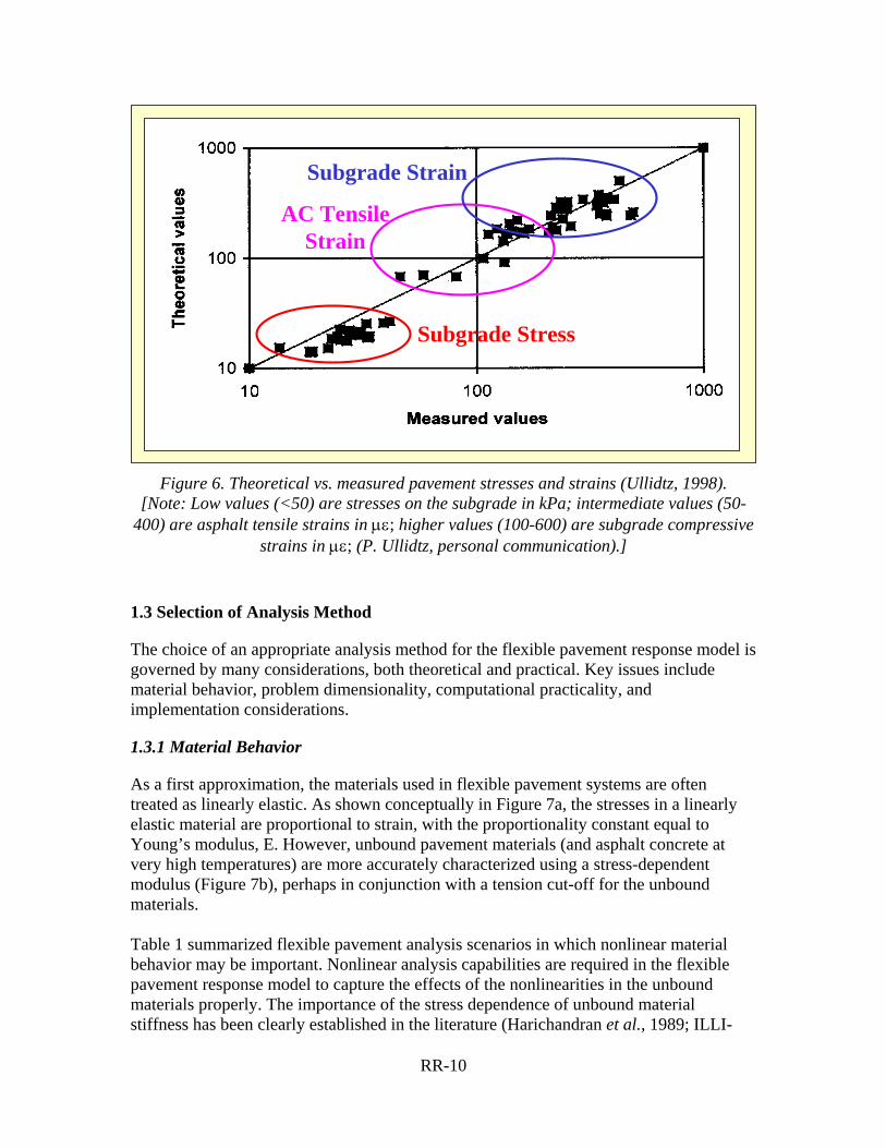
the induced stresses measured by the stress cells were nearly 50% less than those predicted by Boussinesq elastic theory (Ullidtz, Askegaard, and Sjolin, 1996). The above caveats notwithstanding, reasonably accurate predictions of pavement structural response are possible in practice. Dai et al.(1987) found excellent agreement between backcalculated (linearly elastic) and measured asphalt tensile strains at MnRoad (Figure 4). Ertman, Larsen, and Ullidtz (1987) found generally good agreement between predicted (nonlinear analysis) and measured vertical subgrade stresses (Figure 5), although the comparisons for transverse and longitudinal subgrade stresses were much poorer (these horizontal stresses were also much smaller in magnitude than the vertical stresses). Figure 6 summarizes comparisons between predicted (nonlinear analysis) and measured subgrade stresses and strains and asphalt strains as obtained from three Danish test road sections under environmental conditions ranging from winter storm to spring thaw conditions to hot summer temperatures (Ullitdtz, 1998). The overall conclusion from this admittedly limited set of validation results is that careful modeling—and in particular, realistic material characterization—can produce reasonably good predictions of expected pavement structural response.

Quantity C.O.VSurface Deflection 9%

Subgrade Compressive Strain 12%

AC Tensile Strain 15% Table 2. Variability among key pavement response parameters as computed using

various linearly elastic static analysis procedures; C.O.V = coefficient of variation. (Chen et al., 1995)

RR-8

Test Pit

Elevation

Plan

Sand

x

Load3 Stress Cells

Figure 2. Sand test pit for comparison of measured vs. predicted stresses.

(Ullidtz, Askegaard, and Sjolin, 1996)

50%?

Measured

Predicted (Boussinesq)

Figure 3. Comparison of measured vs. predicted stresses for sand test pit.

(Ullidtz, Askegaard, and Sjolin, 1996)

RR-9

(EVERCALC)

MnROAD(Dai et al., 1987)

Figure 4. Comparisons between backcalculated and measured asphalt tension strains at

MnRoad (Dai et al., 1987).

Danish Test RoadDanish Test Road

0

50

100

150

kPa

1 2 3

Layer

Vertical Subgrade Stress

Gauge 1 Gauge 2 Calculated

0

5

10

15

kPa

1 2 3

Layer

Transverse Subgrade Stress

-2

0

2

4

6

8

kPa

1 2 3

Layer

Longitudinal Subgrade Stress

(Ertman Larsen and Ullidtz, 1987)

FWD Load on AC

Figure 5. Comparisons between predicted and measured subgrade stresses at the Danish

test road (Ertman, Larsen, and Ullidtz, 1987).

RR-10

Subgrade Stress

AC TensileStrain

Subgrade Strain

Figure 6. Theoretical vs. measured pavement stresses and strains (Ullidtz, 1998).

[Note: Low values (<50) are stresses on the subgrade in kPa; intermediate values (50-400) are asphalt tensile strains in µε; higher values (100-600) are subgrade compressive

strains in µε; (P. Ullidtz, personal communication).]

1.3 Selection of Analysis Method

The choice of an appropriate analysis method for the flexible pavement response model is governed by many considerations, both theoretical and practical. Key issues include material behavior, problem dimensionality, computational practicality, and implementation considerations.

1.3.1 Material Behavior

As a first approximation, the materials used in flexible pavement systems are often treated as linearly elastic. As shown conceptually in Figure 7a, the stresses in a linearly elastic material are proportional to strain, with the proportionality constant equal to Young’s modulus, E. However, unbound pavement materials (and asphalt concrete at very high temperatures) are more accurately characterized using a stress-dependent modulus (Figure 7b), perhaps in conjunction with a tension cut-off for the unbound materials. Table 1 summarized flexible pavement analysis scenarios in which nonlinear material behavior may be important. Nonlinear analysis capabilities are required in the flexible pavement response model to capture the effects of the nonlinearities in the unbound materials properly. The importance of the stress dependence of unbound material stiffness has been clearly established in the literature (Harichandran et al., 1989; ILLI-

RR-11

PAVE, 1990; Asphalt Institute, 1991; Huang, 1993; Zaghoul and White, 1993; Chen et al. 1995; and Schwartz, 2001 are just a few examples). Figure 8 and Table 3 summarize results from Chen et al. (1995) that provide some quantitative insights into the effects of unbound nonlinear behavior on key pavement response parameters. Ullidtz (1998) also suggests the influence of nonlinear unbound material behavior on pavement response in the field for the Danish test road. He attributes the 40 to 50% discrepancies between the measured subgrade strains and those predicted by three different linearly elastic response models (Figure 9) to the neglect of nonlinear subgrade behavior in the predictions. The importance of unbound material nonlinearity--and the issue of how to define an “equivalent” linear analysis for comparison, is discussed in more detail later in Section 4.4.2. Explicit consideration of the rate dependence of asphalt concrete requires viscoelastic analysis capabilities. However, this is not needed for the 2002 Design Guide, where rate effects are incorporated by adjusting the AC stiffness using the complex modulus master curve.

E = f (Stress)

E = constant

Stress

Strain

(a) Linear

Stress

Strain

(b) Nonlinear Figure 7. Nonlinear material behavior.

RR-12

MICH-PAVE

LinearNonlinear

Figure 8. Example of influence of nonlinear unbound material on predicted surface

deflections (Chen et al., 1995).

Range MeanSurface Deflection 0.6-18.8% 5.5%

Subgrade Compressive Strain 0.6-20.6% 7.6%

AC Tensile Strain 0-7.2% 1.3%

DifferencesQuantity

Table 3. Differences between linear and nonlinear analyses as reported by Chen et al.

(1995).

RR-13

Nonlinearity?

Figure 9. Comparison of measured subgrade vertical strain against predictions from

linearly elastic pavement response models (Ullidtz, 1998).

1.3.2 Problem Dimensionality

The required dimensionality (1D vs. 2D vs. 3D) of an analysis is a function of geometry and loading conditions. Table 1 summarized flexible pavement analysis scenarios in which three-dimensional geometric effects may be important. The issue of two- vs. three-dimensional finite element analysis for flexible pavements has become quite controversial in recent years (GAO, 19971) and has been addressed head-on in this project. The issue is not whether we can perform three-dimensional finite element analyses for pavements, including nonlinear material behavior and dynamic response, if necessary; clearly, these types of analyses are well within the capabilities of any number of available finite element programs. The real issue is whether we should implement these capabilities for design, and in particular for the flexible pavement design formulation proposed for the 2002 Design Guide. In most flexible pavement problems, there are no vertical discontinuities (e.g., slab joints) and the only source of three-dimensionality is multiple wheel loads. If the behavior of all materials in the pavement structure can be treated as linear, then a 3D solution can be constructed from simpler 2D axisymmetric analysis results via superposition. Although nonlinear material behavior invalidates the principle of superposition from a rigorously theoretical standpoint, superposition may still provide acceptably accurate calculations of

1 The GAO report recommended that “nonlinear 3D-FEM is considered in the current update of the pavement design guide.” The GAO report was based principally upon interviews with selected members of the University and government pavement research community and is not an in-depth peer-reviewed study.

RR-14

critical pavement response parameters in most pavement structures (Schwartz, 2000). This is discussed further in a later section. Discrete vertical discontinuities are important three-dimensional geometrical features in some flexible and composite pavement rehabilitation scenarios, in particular with regard to reflection cracking. These vertical discontinuities invalidate the two-dimensional assumption of axial symmetry. However, reflection cracking has been excluded from the scope of the 2002 Design Guide and, as a consequence, modeling of vertical boundaries/discontinuities is not required and a 2D axisymmetric analysis will be sufficient from a geometrical viewpoint.

1.3.3 Computational Practicality

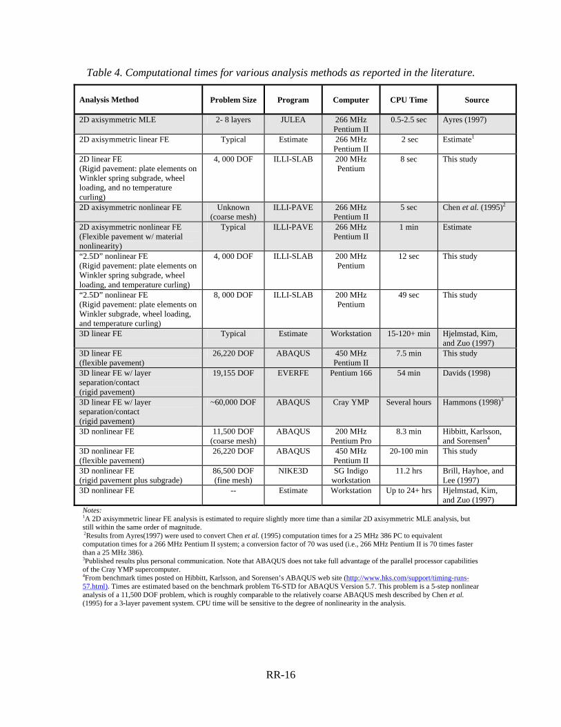
It must be recognized that the type of flexible pavement FEA required for the purposes of the 2002 Design Guide are not complex. They consist of regular meshes, simple material models with relatively gentle nonlinearities, and straightforward monotonic loadings.2 The key difficulty lies in the large number of analyses required for the incremental damage/reliability design formulations implemented in the guide. The pavement response model must be able to perform all analysis calculations in a practically acceptable amount of time. The time required to perform a flexible pavement response analysis is a complex function of the type of analysis methodology (e.g., MLET vs. FEM), the dimensionality of the problem (e.g., 2D vs. 3D), the complexity of the pavement structure, the degree of material nonlinearity to be considered, and computer type and speed. Very broad estimates of required calculation times on current generation personal computers can be summarized as follows (see Table 4 for details):

- 2D linear analyses (MLET/FEM): Seconds - 2D nonlinear FE analyses: 10s of seconds - 3D linear FE analyses: 10s of minutes to hours - 3D nonlinear FE analyses: Hours to 10s of hours

Although today we clearly can perform theoretically rigorous 3D finite element analyses that incorporate a rich set of sophisticated modeling features, computational practicality—i.e., the ability to perform the calculations in an acceptable amount of time—will nonetheless remain a major constraint on whether we will perform them for routine design (as opposed to research). Quibbling whether a 3D analysis requires 1 hour or 5 hours does not alter the fact that these computations, when performed with adequate levels of mesh refinement and modeling detail, require non-trivial solution times in the computer environments found in practice today or expected in the near future.

2 This is not to imply that all pavement finite element calculations are simple. Modeling of cyclic traffic loading with nonlinear material models, characterization of material degradation and fracturing at reflection cracks, and dynamic analysis under moving vehicle loads are challenging problems that are at or beyond the limit of current capabilities. However, none of these advanced features is required for the 2002 Design Guide.

RR-15

Note that the broad time estimates given above are for a single analysis. The distress/damage accumulation schemes incorporated in the 2002 Design Guide require a separate incremental damage analysis for each vehicle category for each season for perhaps multiple years. A design analysis based on 12 seasons per year and a 20 year design life may require 240 separate finite element solutions. A Monte Carlo-based reliability solution may require hundreds of simulations of the pavement design life. Thus, many thousands of finite element solutions may be required for a single pavement design. Clearly, each solution can take no more than a few seconds under this scenario. Three-dimensional analyses are clearly impractical for these types of design analyses. The computational speed of the design calculations can in concept be improved by fitting a regression or neural network model to a set of analytically generated parametric results. This is the approach adopted for the rigid pavement response model in the 2002 Design Guide. Unfortunately, the much larger set of input variables for flexible pavements makes this neural network approach impractical.

RR-16

Table 4. Computational times for various analysis methods as reported in the literature.

Analysis Method

Problem Size

Program

Computer

CPU Time

Source

2D axisymmetric MLE 2- 8 layers JULEA 266 MHz Pentium II

0.5-2.5 sec Ayres (1997)

2D axisymmetric linear FE Typical Estimate 266 MHz Pentium II

2 sec Estimate1

2D linear FE (Rigid pavement: plate elements on Winkler spring subgrade, wheel loading, and no temperature curling)

4, 000 DOF ILLI-SLAB

200 MHz Pentium

8 sec This study

2D axisymmetric nonlinear FE Unknown (coarse mesh)

ILLI-PAVE 266 MHz Pentium II

5 sec Chen et al. (1995)2

2D axisymmetric nonlinear FE (Flexible pavement w/ material nonlinearity)

Typical ILLI-PAVE 266 MHz Pentium II

1 min Estimate

“2.5D” nonlinear FE (Rigid pavement: plate elements on Winkler spring subgrade, wheel loading, and temperature curling)

4, 000 DOF ILLI-SLAB

200 MHz Pentium

12 sec This study

“2.5D” nonlinear FE (Rigid pavement: plate elements on Winkler subgrade, wheel loading, and temperature curling)

8, 000 DOF ILLI-SLAB

200 MHz Pentium

49 sec This study

3D linear FE Typical Estimate Workstation 15-120+ min Hjelmstad, Kim, and Zuo (1997)

3D linear FE (flexible pavement)

26,220 DOF ABAQUS 450 MHz Pentium II

7.5 min This study

3D linear FE w/ layer separation/contact (rigid pavement)

19,155 DOF EVERFE Pentium 166 54 min Davids (1998)

3D linear FE w/ layer separation/contact (rigid pavement)

~60,000 DOF ABAQUS Cray YMP Several hours Hammons (1998)3

3D nonlinear FE 11,500 DOF (coarse mesh)

ABAQUS 200 MHz Pentium Pro

8.3 min Hibbitt, Karlsson, and Sorensen4

3D nonlinear FE (flexible pavement)

26,220 DOF ABAQUS 450 MHz Pentium II

20-100 min This study

3D nonlinear FE (rigid pavement plus subgrade)

86,500 DOF (fine mesh)

NIKE3D SG Indigo workstation

11.2 hrs Brill, Hayhoe, and Lee (1997)

3D nonlinear FE -- Estimate Workstation Up to 24+ hrs Hjelmstad, Kim, and Zuo (1997)

Notes: 1A 2D axisymmetric linear FE analysis is estimated to require slightly more time than a similar 2D axisymmetric MLE analysis, but still within the same order of magnitude. 2Results from Ayres(1997) were used to convert Chen et al. (1995) computation times for a 25 MHz 386 PC to equivalent computation times for a 266 MHz Pentium II system; a conversion factor of 70 was used (i.e., 266 MHz Pentium II is 70 times faster than a 25 MHz 386). 3Published results plus personal communication. Note that ABAQUS does not take full advantage of the parallel processor capabilities of the Cray YMP supercomputer. 4From benchmark times posted on Hibbitt, Karlsson, and Sorensen’s ABAQUS web site (http://www.hks.com/support/timing-runs-57.html). Times are estimated based on the benchmark problem T6-STD for ABAQUS Version 5.7. This problem is a 5-step nonlinear analysis of a 11,500 DOF problem, which is roughly comparable to the relatively coarse ABAQUS mesh described by Chen et al. (1995) for a 3-layer pavement system. CPU time will be sensitive to the degree of nonlinearity in the analysis.

RR-17

1.3.3.1 Some Factors Influencing Analysis Times for Pavement Scenarios

Conventional wisdom holds that axisymmetric multilayer elastic theory solutions (MLET) are less computation-intensive than axisymmetric two-dimensional linear finite element (FE) solutions. However, upon closer examination it is not clear how substantial this disparity will be for realistic pavement design scenarios. The execution time for MLET solutions will increase with number of layers and with number of required stress computation points (e.g., to determine the critical locations for the critical response parameters, and for superposition of multi-wheel loading cases). In contrast, a FE solution (assuming a sufficiently fine mesh) will not require significant additional computation time as the number of layers and/or stress computation points increases. The finite element meshing already divides the pavement structure into many thin layers (theoretically, each layer of elements in the mesh could be assigned properties corresponding to different pavement layers) and the FE algorithms automatically determine the stresses and strains at all element integration points. The primary objective of the study described in this section was to determine the extent to which the conventional wisdom regarding relative computation times is, in fact, correct. Secondly, the study provided quantitative estimates for execution times for the types of MLET and FE flexible pavement analyses envisioned for the 2002 Design Guide. These estimates were particularly important for evaluating how reliability estimates might be incorporated into the design guide methodology. The study also provided additional insights into finite element mesh design guidelines for efficient pavement design analyses. It should be noted that this timing study was performed early during the NCHRP 1-37A project. The results are provided here in part to document the work performed during the project. The more significant reason, however, is that the insights drawn from the results have value beyond just the limited objectives of the study.

Multilayer Elastic Theory Solutions

KENLAYER (Huang, 1993) was used initially to evaluate the execution time requirements for multilayer elastic theory. Analyses were performed for 3, 5, 7, and 9 layer systems loaded with a dual tandem tire configuration. Stress calculation points were evaluated at depths corresponding to the top of each layer. The number of radial locations at each depth for stress calculations was varied in the analyses. All execution times are based on a 450 MHz Pentium II processor. The results from the KENLAYER analyses are summarized in Figure 10. Computation times ranged from very short (less than 1 second) to up to 25 seconds for a 9-layer system with 35 stress computation points per layer. In the MLET algorithms, the computations for a given depth theoretically should only need to be performed once, and then these results can be used repeatedly to evaluate

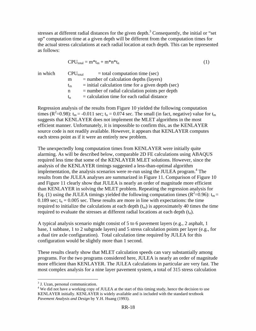
RR-18

stresses at different radial distances for the given depth.3 Consequently, the initial or “set up” computation time at a given depth will be different from the computation times for the actual stress calculations at each radial location at each depth. This can be represented as follows: CPUtotal = m*tm + m*n*tn (1) in which CPUtotal = total computation time (sec) m = number of calculation depths (layers) tm = initial calculation time for a given depth (sec) n = number of radial calculation points per depth tn = calculation time for each radial distance Regression analysis of the results from Figure 10 yielded the following computation times (R2=0.98): tm = -0.011 sec; tn = 0.074 sec. The small (in fact, negative) value for tm suggests that KENLAYER does not implement the MLET algorithms in the most efficient manner. Unfortunately, it is impossible to confirm this, as the KENLAYER source code is not readily available. However, it appears that KENLAYER computes each stress point as if it were an entirely new problem. The unexpectedly long computation times from KENLAYER were initially quite alarming. As will be described below, comparable 2D FE calculations using ABAQUS required less time that some of the KENLAYER MLET solutions. However, since the analysis of the KENLAYER timings suggested a less-than-optimal algorithm implementation, the analysis scenarios were re-run using the JULEA program.4 The results from the JULEA analyses are summarized in Figure 11. Comparison of Figure 10 and Figure 11 clearly show that JULEA is nearly an order of magnitude more efficient than KENLAYER in solving the MLET problem. Repeating the regression analysis for Eq. (1) using the JULEA timings yielded the following computation times (R2=0.96): tm = 0.189 sec; tn = 0.005 sec. These results are more in line with expectations: the time required to initialize the calculations at each depth (tm) is approximately 40 times the time required to evaluate the stresses at different radial locations at each depth (tn). A typical analysis scenario might consist of 5 to 6 pavement layers (e.g., 2 asphalt, 1 base, 1 subbase, 1 to 2 subgrade layers) and 5 stress calculation points per layer (e.g., for a dual tire axle configuration). Total calculation time required by JULEA for this configuration would be slightly more than 1 second. These results clearly show that MLET calculation speeds can vary substantially among programs. For the two programs considered here, JULEA is nearly an order of magnitude more efficient than KENLAYER. The JULEA calculations in particular are very fast. The most complex analysis for a nine layer pavement system, a total of 315 stress calculation

3 J. Uzan, personal communication. 4 We did not have a working copy of JULEA at the start of this timing study, hence the decision to use KENLAYER initially. KENLAYER is widely available and is included with the standard textbook Pavement Analysis and Design by Y.H. Huang (1993).

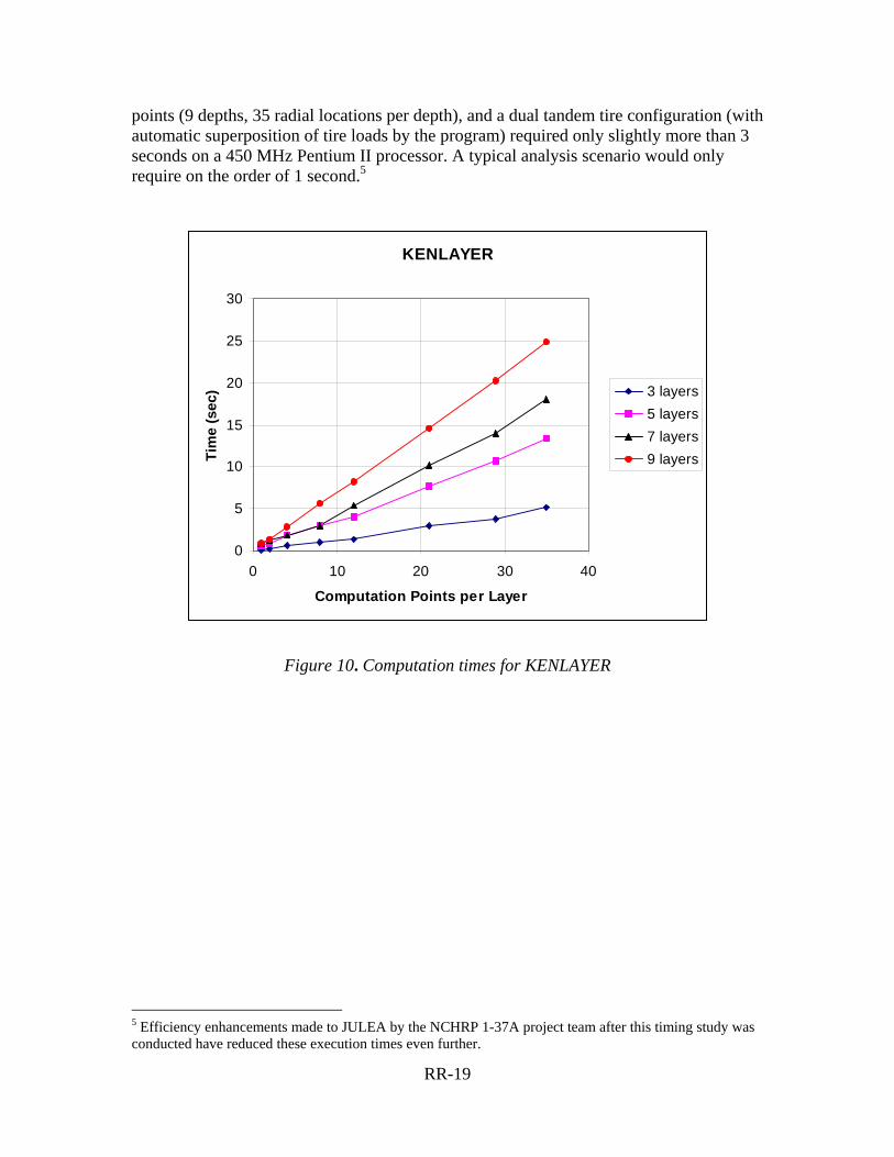
RR-19

points (9 depths, 35 radial locations per depth), and a dual tandem tire configuration (with automatic superposition of tire loads by the program) required only slightly more than 3 seconds on a 450 MHz Pentium II processor. A typical analysis scenario would only require on the order of 1 second.5

KENLAYER

0

5

10

15

20

25

30

0 10 20 30 40

Computation Points per Layer

Tim

e (s

ec) 3 layers

5 layers7 layers9 layers

Figure 10. Computation times for KENLAYER

5 Efficiency enhancements made to JULEA by the NCHRP 1-37A project team after this timing study was conducted have reduced these execution times even further.

RR-20

JULEA

0

5

10

15

20

25

30

0 10 20 30 40

Calculation Points per Layer

3 layer5 layer7 layer9 layer

Figure 11. Computation times for JULEA

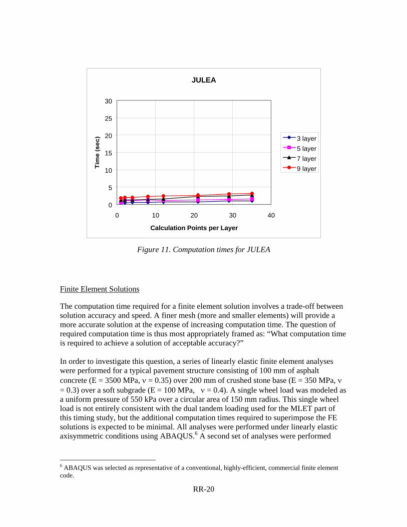
Finite Element Solutions

The computation time required for a finite element solution involves a trade-off between solution accuracy and speed. A finer mesh (more and smaller elements) will provide a more accurate solution at the expense of increasing computation time. The question of required computation time is thus most appropriately framed as: “What computation time is required to achieve a solution of acceptable accuracy?” In order to investigate this question, a series of linearly elastic finite element analyses were performed for a typical pavement structure consisting of 100 mm of asphalt concrete (E = 3500 MPa, ν = 0.35) over 200 mm of crushed stone base (E = 350 MPa, ν = 0.3) over a soft subgrade (E = 100 MPa, ν = 0.4). A single wheel load was modeled as a uniform pressure of 550 kPa over a circular area of 150 mm radius. This single wheel load is not entirely consistent with the dual tandem loading used for the MLET part of this timing study, but the additional computation times required to superimpose the FE solutions is expected to be minimal. All analyses were performed under linearly elastic axisymmetric conditions using ABAQUS.6 A second set of analyses were performed

6 ABAQUS was selected as representative of a conventional, highly-efficient, commercial finite element code.

RR-21

using LS-DYNA7 to compare execution times for implicit vs. explicit finite element formulations, respectively. Three separate but similar finite element meshes were developed to investigate the trade-off between accuracy and speed: 1. A coarse refinement mesh consisting of 396 elements, with a smallest element size of

50 mm by 50 mm (Figure 12). Two elements spanned the thickness of the asphalt concrete surface layer and four elements spanned the thickness of the base layer.

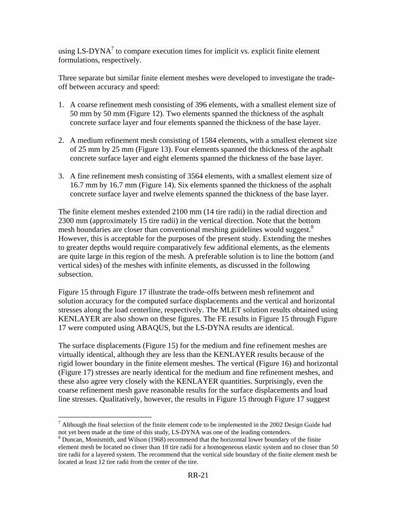
2. A medium refinement mesh consisting of 1584 elements, with a smallest element size of 25 mm by 25 mm (Figure 13). Four elements spanned the thickness of the asphalt concrete surface layer and eight elements spanned the thickness of the base layer.

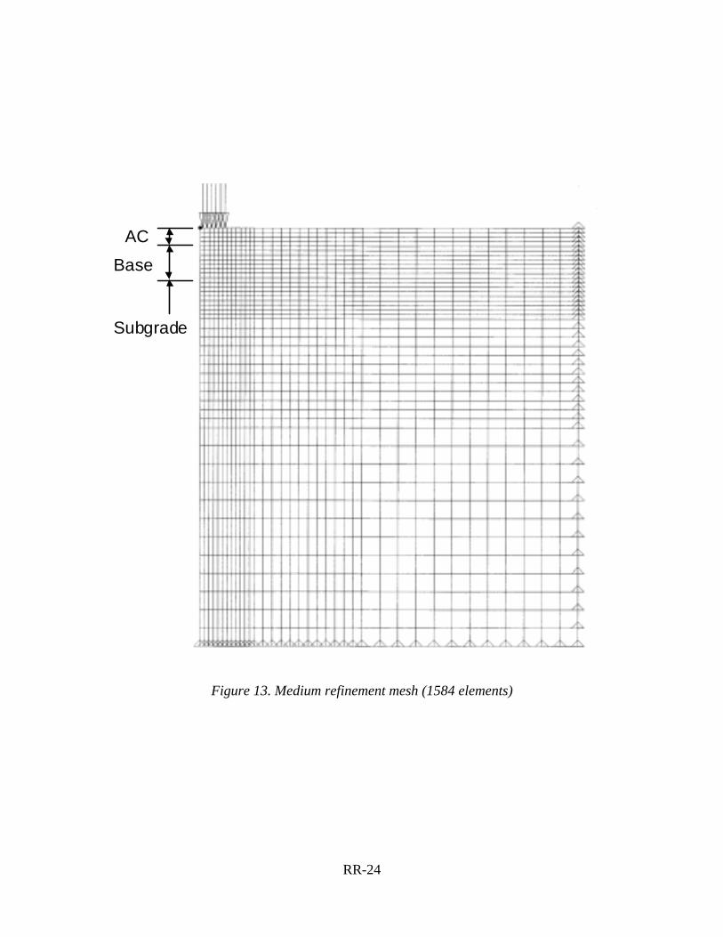
3. A fine refinement mesh consisting of 3564 elements, with a smallest element size of 16.7 mm by 16.7 mm (Figure 14). Six elements spanned the thickness of the asphalt concrete surface layer and twelve elements spanned the thickness of the base layer.

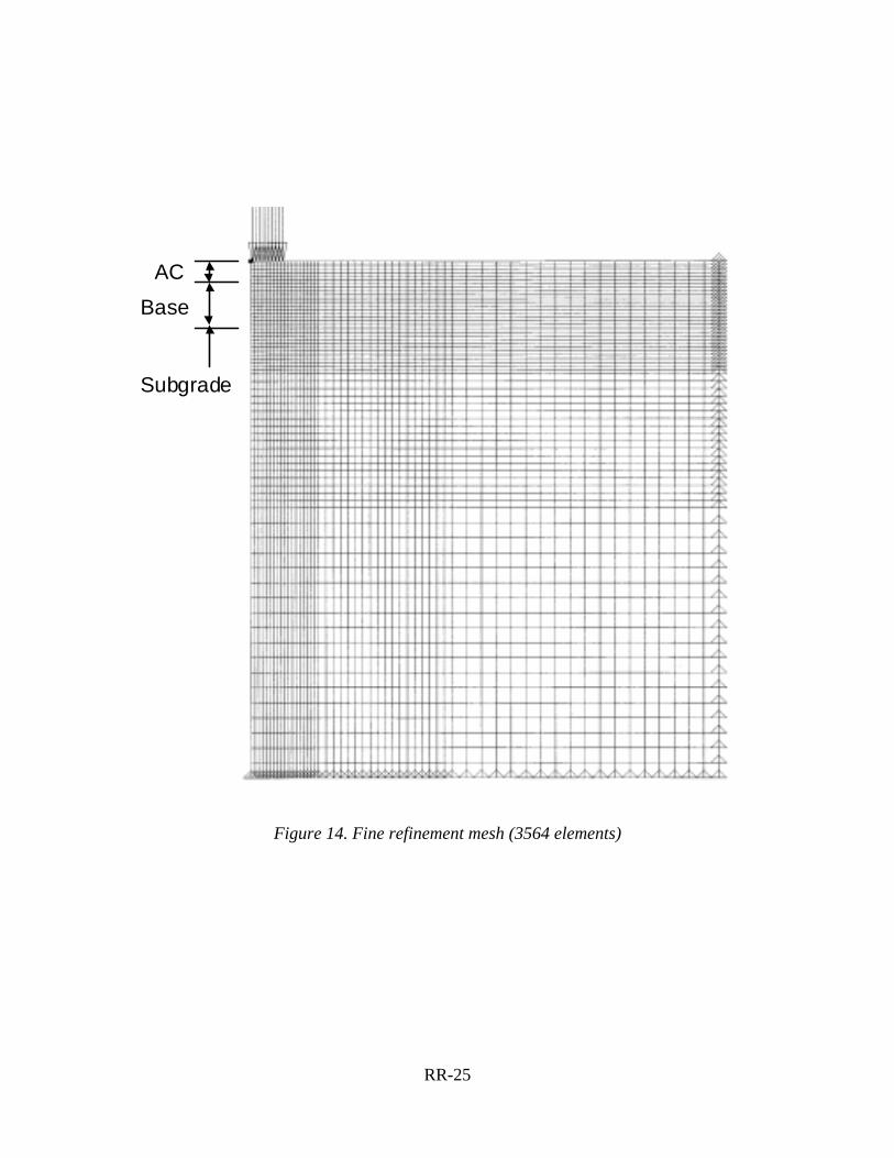
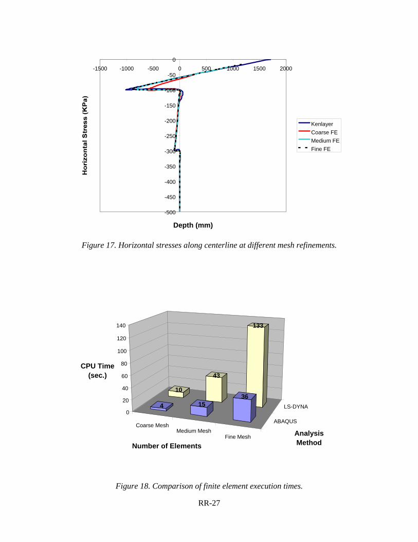
The finite element meshes extended 2100 mm (14 tire radii) in the radial direction and 2300 mm (approximately 15 tire radii) in the vertical direction. Note that the bottom mesh boundaries are closer than conventional meshing guidelines would suggest.8 However, this is acceptable for the purposes of the present study. Extending the meshes to greater depths would require comparatively few additional elements, as the elements are quite large in this region of the mesh. A preferable solution is to line the bottom (and vertical sides) of the meshes with infinite elements, as discussed in the following subsection. Figure 15 through Figure 17 illustrate the trade-offs between mesh refinement and solution accuracy for the computed surface displacements and the vertical and horizontal stresses along the load centerline, respectively. The MLET solution results obtained using KENLAYER are also shown on these figures. The FE results in Figure 15 through Figure 17 were computed using ABAQUS, but the LS-DYNA results are identical. The surface displacements (Figure 15) for the medium and fine refinement meshes are virtually identical, although they are less than the KENLAYER results because of the rigid lower boundary in the finite element meshes. The vertical (Figure 16) and horizontal (Figure 17) stresses are nearly identical for the medium and fine refinement meshes, and these also agree very closely with the KENLAYER quantities. Surprisingly, even the coarse refinement mesh gave reasonable results for the surface displacements and load line stresses. Qualitatively, however, the results in Figure 15 through Figure 17 suggest

7 Although the final selection of the finite element code to be implemented in the 2002 Design Guide had not yet been made at the time of this study, LS-DYNA was one of the leading contenders. 8 Duncan, Monismith, and Wilson (1968) recommend that the horizontal lower boundary of the finite element mesh be located no closer than 18 tire radii for a homogeneous elastic system and no closer than 50 tire radii for a layered system. The recommend that the vertical side boundary of the finite element mesh be located at least 12 tire radii from the center of the tire.

RR-22

that, of the three meshes studied, the medium refinement (1584 elements, with 4 element layers in the AC and 3 element layers in the base) mesh is the minimum refinement necessary to achieve acceptable solution accuracy. The execution times for all three meshes are summarized in Figure 18 for both the ABAQUS (implicit formulation) and LS-DYNA (explicit formulation) programs. For the medium refinement mesh (1584 elements), ABAQUS required 15 CPU seconds while LS-DYNA required 43 CPU seconds. As before, all times are based on a 450 MHz Pentium II process with 256 MB of RAM. Execution times would be slightly longer for a deeper lower mesh boundary. Although quite short, the ABAQUS times are still approximately an order of magnitude greater than the time required to analyze a typical pavement scenario using JULEA. The LS-DYNA computations typically take about three times longer than the corresponding ABAQUS analysis. However, this disparity between ABAQUS and LS-DYNA would be expected to decrease for nonlinear analyses, where the time for the implicit formulation in ABAQUS would increase disproportionately with respect to the explicit formulation in LS-DYNA.

RR-23

Subgrade

Base

AC

Figure 12. Coarse refinement mesh (396 elements)

RR-24

Subgrade

Base

AC

Figure 13. Medium refinement mesh (1584 elements)

RR-25

Subgrade

Base

AC

Figure 14. Fine refinement mesh (3564 elements)

RR-26

-0.05

0

0.05

0.1

0.15

0.2

0.25

0.3

0.35

0.4

0.45

0 500 1000 1500 2000 2500

Radial Distance (mm)

KenlayerMedium FECoarse FEFine FE

Figure 15. Surface displacements computed at different mesh refinements.

-500

-450

-400

-350

-300

-250

-200

-150

-100

-50

00 100 200 300 400 500 600 700 800

Depth (mm)

KenlayerCoarse FEMedium FEFine FE

Figure 16. Vertical stresses along centerline at different mesh refinements.

RR-27

-500

-450

-400

-350

-300

-250

-200

-150

-100

-50

0-1500 -1000 -500 0 500 1000 1500 2000

Depth (mm)

KenlayerCoarse FEMedium FEFine FE

Figure 17. Horizontal stresses along centerline at different mesh refinements.

Coarse MeshMedium Mesh

Fine Mesh

ABAQUS

LS-DYNA

10

43

133

4 1536

0

20

40

60

80

100

120

140

CPU Time (sec.)

Number of Elements

Analysis Method

Figure 18. Comparison of finite element execution times.

RR-28

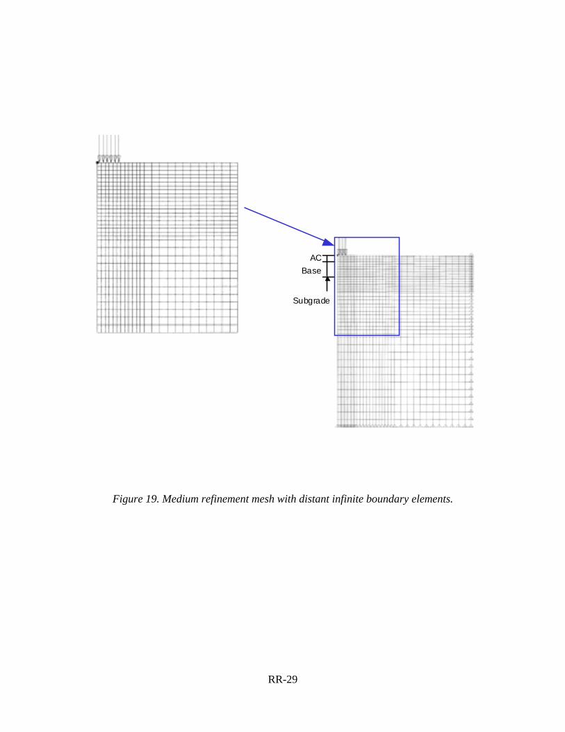
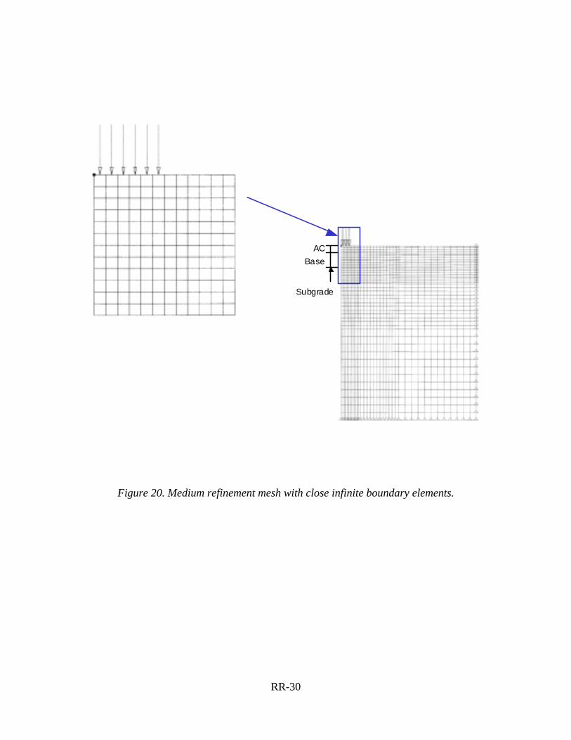
Infinite Boundary Elements

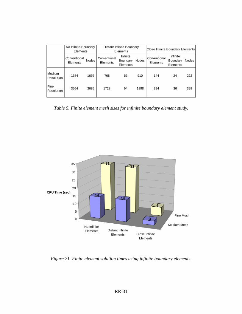
The types of finite element models required for flexible pavement design as envisioned in the 2002 Design Guide are not complex. They consist of regular meshes, simple material models with at most only relatively gentle nonlinearities, and straightforward monotonic quasi-static loadings. The major practical difficulty is the large mesh sized dictated by the need to locate the bottom and side boundaries of the mesh far from the vehicle loads. This is not an important issue for a single analysis, but it becomes a major drawback for reliability-based incremental damage design procedures. One method for decreasing the computation time of pavement finite element analyses is to use infinite boundary elements to replace all of the far field elements that serve only to link the zone of interest in the immediate vicinity of the wheel loads (where stress and strain gradients are largest and where any material nonlinearity will be most evident) to the distant mesh boundaries. The medium and fine refinement meshes in Figure 13 and Figure 14 were therefore modified to include infinite boundary elements at two different distances from the wheel loads. For example Figure 19 depicts the infinite boundary elements located relatively far from the wheel loads in the medium refinement mesh, while Figure 20 shows the infinite boundary elements relatively close to the wheel loads for the same medium refinement meshes. These cases are reasonable bounding cases for the location of the infinite elements. The numbers of elements and nodes in each mesh are summarized in Table 5. The meshes incorporating the infinite boundary elements were reanalyzed using ABAQUS. The execution times for all cases are summarized in Figure 21. As before, all times are based on a 450 MHz Pentium II processor with 256 MB of RAM. The cases with the infinite boundary elements located relatively far from the wheel loads provided little or no benefit in reducing computation times; the extra computational overhead involved with the infinite boundary elements negates the savings from reducing the number of conventional quadrilateral elements. On the other hand, the cases with the infinite boundary elements located relatively near the wheel loads reduced the total computation time by a factor of 5. Under these conditions, the FE solution is only 2 to 3 times more time consuming that a corresponding MLET solution for a typical pavement scenario. Although this is still consistent with the conventional wisdom that MLET solutions are less computation-intensive than a corresponding FE analysis, it also clearly indicates that the differences in the computational demands are not nearly as great as many assume.

RR-29

Subgrade

BaseAC

Figure 19. Medium refinement mesh with distant infinite boundary elements.

RR-30

Subgrade

BaseAC

Figure 20. Medium refinement mesh with close infinite boundary elements.

RR-31

Conventional Elements Nodes

Conventional Elements

Infinite Boundary Elements

NodesConventional

Elements

Infinite Boundary Elements

Nodes

Medium Resolution

1584 1665 768 56 910 144 24 222

Fine Resolution

3564 3685 1728 94 1898 324 36 398

No Infinite Boundary Elements

Distant Infinite Boundary Elements Close Infinite Boundary Elements

Table 5. Finite element mesh sizes for infinite boundary element study.

No InfiniteElements Distant Infinite

Elements Close InfiniteElements

Medium Mesh

Fine Mesh

3131

6

1414

30

5

10

15

20

25

30

35

CPU Time (sec)

Figure 21. Finite element solution times using infinite boundary elements.

RR-32

Conclusions from Timing Study

Recall that this timing study was performed early during the NCHRP 1-37A project, largely to address some early questions regarding the overall formulation of the flexible pavement analysis system. However, the insights drawn from the results have value beyond just the limited objectives of the study. Principle findings include: • MLET calculation speeds can vary substantially among programs. JULEA is nearly

an order of magnitude more efficient than KENLAYER.

• The JULEA calculations are very fast. A typical flexible pavement design scenario would require on the order of 1 second or less per analysis.

• Execution times for ABAQUS FE solutions (without use of infinite boundary elements) are approximately an order of magnitude longer than the time required for a typical pavement analysis scenario using JULEA.

• Execution times for LS-DYNA FE solutions (explicit FE formulation) are approximately three times longer than the FE solution times using ABAQUS (implicit FE formulation).

• Use of infinite boundary elements to model the far-field regions can reduce the FE solution times by up to a factor of 5.

• Linearly elastic FE solutions incorporating infinite boundary elements may only be as little as 2 to 3 times slower than a corresponding MLET analysis using JULEA.

All FE solutions in this study were for linearly elastic conditions. Although not quantified in this timing study, incorporation of unbound material nonlinearity in the FE solutions will increase the required analysis execution times.

Addendum

The timing study reported in this section was conducted before the DSC2D finite element code had been selected for the pavement response model. Limited timing studies were repeated after the DSC2D code was selected for comparison with the ABAQUS execution times. Timing comparisons between DSC2D and ABAQUS for linearly elastic conditions and no infinite boundary elements are summarized in Table 6. The data clearly show that the DSC2D code is at least as fast, and in some cases faster, than ABAQUS. In addition, some nonlinear analyses were performed using the nonlinear resilient modulus model implemented in the DSC2D code. The analysis times per load increment for the nonlinear analyses were only about 10 to 20% longer than for the corresponding linear analysis cases. Of course, nonlinear analyses will in general have multiple load increments while the linear analyses have only one.

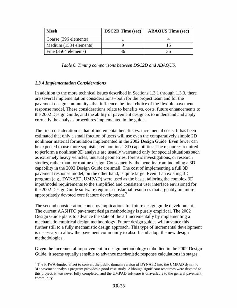
RR-33

Mesh DSC2D Time (sec) ABAQUS Time (sec)

Coarse (396 elements) 1 4 Medium (1584 elements) 9 15 Fine (3564 elements) 36 36

Table 6. Timing comparisons between DSC2D and ABAQUS.

1.3.4 Implementation Considerations

In addition to the more technical issues described in Sections 1.3.1 through 1.3.3, there are several implementation considerations--both for the project team and for the pavement design community--that influence the final choice of the flexible pavement response model. These considerations relate to benefits vs. costs, future enhancements to the 2002 Design Guide, and the ability of pavement designers to understand and apply correctly the analysis procedures implemented in the guide. The first consideration is that of incremental benefits vs. incremental costs. It has been estimated that only a small fraction of users will use even the comparatively simple 2D nonlinear material formulation implemented in the 2002 Design Guide. Even fewer can be expected to use more sophisticated nonlinear 3D capabilities. The resources required to perform a nonlinear 3D analysis are usually warranted only for special situations such as extremely heavy vehicles, unusual geometries, forensic investigations, or research studies, rather than for routine design. Consequently, the benefits from including a 3D capability in the 2002 Design Guide are small. The cost of implementing a full 3D pavement response model, on the other hand, is quite large. Even if an existing 3D program (e.g., DYNA3D, UMPAD) were used as the basis, tailoring the complex 3D input/model requirements to the simplified and consistent user interface envisioned for the 2002 Design Guide software requires substantial resources that arguably are more appropriately devoted core feature development.9 The second consideration concerns implications for future design guide development. The current AASHTO pavement design methodology is purely empirical. The 2002 Design Guide plans to advance the state of the art incrementally by implementing a mechanistic-empirical design methodology. Future design guides will advance this further still to a fully mechanistic design approach. This type of incremental development is necessary to allow the pavement community to absorb and adopt the new design methodologies. Given the incremental improvement in design methodology embodied in the 2002 Design Guide, it seems equally sensible to advance mechanistic response calculations in stages. 9 The FHWA-funded effort to convert the public domain version of DYNA3D into the UMPAD dynamic 3D pavement analysis program provides a good case study. Although significant resources were devoted to this project, it was never fully completed, and the UMPAD software is unavailable to the general pavement community.

RR-34

The current state-of-practice relies (at best) on multilayer elastic theory. The next logical increment is to move to “simple”--i.e., 2D static linear/nonlinear--finite element analysis. The final increment to a full 3D nonlinear analysis capability then can occur in some future revision to the design guide, after the pavement community has already developed a comfort level with the simpler finite element formulations. It is important to recognize the implementing a 2D finite element formulation in the 2002 Design Guide does not hinder implementation of a full 3D formulation in the future. Indeed, in terms of user acceptance, it will help smooth the way for this future implementation. From a technical viewpoint, the finite element pavement response model is implemented in the 2002 Design Guide software as an interchangeable module that can be readily removed and replaced or enhanced in the future to incorporate new advances in the state of the art. Future 3D finite element programs will be better, faster, and cheaper than current programs. It seems prudent to wait and capitalize on these future improvements rather than to implement a lesser program now when it is not really needed. A final consideration is the “transparency” of the pavement response model--i.e., how well users can examine and understand its internal workings. The flexible pavement response model in the 2002 Design Guide is designed so that it can be used as a “black box”. However, the pavement design end users must be encouraged to get “inside the box” and develop a deeper understanding of the analysis methodology. If users find that the inside of the box is needlessly complex (e.g., 3D nonlinear dynamic algorithms), they will be discouraged and perhaps even abandon their attempt. Keeping the pavement response model as “complex as necessary, but no more”10 will help minimize this problem.

1.3 Summary of Finite Element Advantages and Disadvantages

Two flexible pavement analysis methods have been implemented in the 2002 Design Guide. For cases in which all materials in the pavement structure can realistically be treated as linearly elastic, the JULEA multilayer elastic theory program is used to determine the pavement response. JULEA provides an excellent combination of analysis features, theoretical rigor, and computational speed for linear pavement analyses. In cases where the unbound material nonlinearity is also considered, the DSC2D nonlinear finite element code is used instead for determining the pavement stresses, strains, and displacements.

10 This is the inverse of Einstein’s famous quotation: “Everything should be made as simple as possible, but no simpler.”

RR-35

A major advantage of MLET solutions is very quick computation times. These method also have the advantage of requiring only minimal input data from the user; the principal inputs consist of the thicknesses and elastic properties of the layers and the tire contact radius and pressure. Solutions for multiple wheel loads can be constructed from the fundamental axisymmetric single wheel solutions via superposition, often automatically by the computer program. The principal disadvantage of MLET solutions is the restriction to linearly elastic material behavior. Real pavement materials, and the unbound materials in particular, often exhibit stress-dependent stiffness. The materials may even reach a failure condition in some locations, such as in tension at the bottom of the unbound base layer in some pavement structures. These nonlinearities vary both through the thickness of the layer and horizontally within the layer. Some attempts have been made to incorporate these material nonlinearity effects into MLET solutions in an approximate way (Asphalt Institute, 1991; Huang, 1993), but the fundamental axisymmetric MLET formulation makes it impossible to include the spatial variation of stiffness in a realistic manner. The axisymmetric formulation also makes it impossible to include any effects of vertical discontinuities in the analysis or to include nonuniform tire contact pressures in a realistic manner. The limitations of MLET solutions are the strengths of FE analysis. Finite elements are not constrained to two-dimensional axisymmetric conditions (although this is all that is required for the 2002 Design Guide), but can be easily used for two-dimensional plane stress/strain and/or generalized to a fully three-dimensional formulation in the future. This enables modeling of discontinuities and realistic nonuniform tire contact pressure distributions. In addition, the finite element method can simulate a wide variety of nonlinear material behavior; the underlying finite element formulation is not constrained to linear elasticity, as is the case with MLET. Stress-dependent stiffness, tension and shear failures, plastic flow, and material damage can all be treated within the finite element framework. Implementation of some of these nonlinear material modeling capabilities for pavement analyses in the 2002 Design Guide is described in a subsequent section. Conversely, the strengths of MLET solutions are the weaknesses of FE analysis. The input required to define the finite element mesh is substantially greater—and more time-consuming to construct—than the data required for a MLET analysis. This can be mitigated somewhat by use of interactive graphics pre- and post-processors for creating the mesh and viewing the results. Finite element analyses also require more computation time than do equivalent MLET solutions. Finite element solution times--even with infinite boundary elements--are still 2 to 5 times longer than corresponding MLET analyses. Based on all of these considerations, it is the overwhelming judgment of the flexible pavement analysis group was that three-dimensional finite element analysis is not

RR-36

appropriate for inclusion in the 2002 Design Guide.11 Some even argued that inclusion of three-dimensional finite analysis might actually diminish the overall quality of the guide and the likelihood of its successful adoption by state agencies. The project team recognizes that there may be special cases in which progressive agencies with sufficient technical expertise will wish to perform 3D finite element analyses, e.g., for specific (local) geometries and loadings and for forensic studies. These types of analyses can already be performed with any of the many excellent commercial 3D finite element codes currently available.

11 The project team is not alone in this assessment. During the 2002 Design Guide workshop at the January 2000 Transportation Research Board Meetings, Dr. Samir Shoukry, organizer of the first two International Conferences of 3D FEM for Pavement Analysis, also voiced the opinion that 3D finite element analysis was not an appropriate tool for routine design.

RR-37

2. SELECTION OF FINITE ELEMENT PROGRAM

Several specialized finite element computer programs for flexible pavements have been developed over the years. The best known of these include ILLI-PAVE (Raad and Figueroa, 1980) and MICH-PAVE (Harichandran, Yeh, and Baladi, 1990). In addition, general-purpose finite element codes like ABAQUS (Hibbitt, Karlsson, and Sorensen, 1998), and DYNA (Livermore Software Technology Corporation, 1999) have also been used for pavement analysis. The project team conducted a careful and thorough evaluation of several leading finite element programs for potential implementation in the guide (Desai and Schwartz, 2000). Three candidate finite element computer programs were initially identified for in-depth evaluation; the NCHRP Project 1-37A panel subsequently requested that a fourth program (UMPAD) also be evaluated:

• ILLI-PAVE (University of Illinois; M.R. Thompson) • DSC2D (University of Arizona; C.S. Desai) • DYNA3D (Lawrence Livermore National Laboratories; J. Hallquist) • UMPAD (Battelle Memorial Institute/FHWA; J. Kennedy)

The ABAQUS general purpose commercial finite element code was also an initial candidate based on its technical capabilities and its extensive past usage in research-oriented pavement analysis. However, the project team eliminated ABAQUS early on because of its high licensing costs and restrictive licensing terms.

2.1 Key Issues

2.1.1 Efficiency Issues

The incremental damage and reliability formulations proposed for the 2002 Design Guide mandate that analysis efficiency be of paramount importance in the selection of an appropriate finite element program for the flexible pavement response model. Consequently, the guiding principle for the flexible pavement response model is that it should be as accurate and sophisticated as it needs to be for the purposes of the 2002 Design Guide and no more. Increasing accuracy and sophistication beyond what is needed can only detract from analysis efficiency. The following points—in decreasing order of importance—will have a major impact on analysis efficiency. 1. Two- vs. three-dimensions: Computation time for a three-dimensional analysis is up

to two to three orders of magnitude longer than for a corresponding two-dimensional calculation (see Section 1.3.3). Input (mesh) preparation and post-processing resource

RR-38

demands (computer and user time, disk space, etc.) are also substantially greater.

2. Static vs. dynamic: Computation time for a dynamic analysis is several orders of magnitude longer than for a corresponding static calculation. There is no compelling reason for performing dynamic analyses in the 2002 Design Guide, especially given the level of idealization/approximation in the other areas of the design approach (e.g., material characterization).

3. Formulation—implicit vs. explicit. For linear static problems, implicit finite element

formulations (e.g., ILLI-PAVE, DSC2D) are faster than a corresponding explicit formulation of the type implemented in DYNA3D.12 This advantage decreases when nonlinear material behavior is introduced, as the computation time for the implicit formulation may increase significantly with nonlinearity (in order to achieve equilibrium convergence iteratively within each load increment) while the time for a corresponding explicit formulation will increase by a smaller extent (pure incremental formulation).

4. Mesh design: There are three major efficiency issues in the design of meshes for pavement problems: • Number of elements or degree of mesh refinement. Fewer elements mean faster

analyses, albeit at degraded solution accuracy. The trade-off between accuracy and solution time can only be established via parametric sensitivity studies. Note that this consideration is not specific to any particular finite element program, but applies equally to all.

• Location of boundary conditions. Conventional wisdom suggests that the vertical side boundaries for the mesh should be no closer than 10 to 12 tire radii; the horizontal bottom boundary at the base of the subgrade should be no closer than 50 tire radii (e.g., see Duncan et al. 1968 and Chen et al. 1995). These minimum distances require meshes having many elements and nodes outside the primary zone of interest, i.e., the highly stressed region beneath the tire load. Special analysis features such as the infinite elements available in many codes (e.g., the dynamic compliant boundaries in UMPAD) can be used effectively to move the boundaries closer and thus reduce the number of elements and nodes.

• Element formulation. Higher order elements (e.g., 8-node quadrilaterals) can be more efficient and therefore require fewer elements than do lower order elements (e.g., 4-node quadrilaterals) for comparable accuracy in linear problems. For nonlinear analyses, more but smaller low-order elements are often more effective than fewer but larger high-order elements for tracking the nonlinear response. The ideal approach is perhaps a hybrid set of elements in which high-order elements are used in the areas of primarily linear response (e.g., the AC layer, and regions of the unbound layers far removed from the loading) and low-order elements are

12 See Bathe (1996) for details regarding implicit and explicit finite element formulations.

RR-39

used in the areas of nonlinear response (e.g., the regions of the unbound layers nearest the loading).

5. Equation solver: In implicit formulations (see Item 3 above), most of the computation

time for larger finite element analysis is spent in solving the system of simultaneous equations. Algorithms are available that can automatically resequence equations to minimize bandwidth or wavefront in order to optimize the computational efficiency of the equation solver. Fortunately, the regular nature of most pavement finite element meshes make optimal node numbering fairly straightforward during mesh design. The equation solver algorithms themselves must also be highly efficient, but fortunately, these routines are widely available today and incorporated in most modern finite element codes.

6. Miscellaneous numerics: This encompasses all of the miscellaneous details of the

finite element algorithms that are related to computational efficiency (e.g., iteration algorithms for implicit formulations, numerical integration, disk I/O operations, etc). For single processor finite element codes, most of these miscellaneous items are of comparatively minor importance to the overall computational efficiency. For multi-processor finite element codes, the degree of parallelism in the algorithms becomes a dominant consideration. However, multi-processor algorithms are not envisioned for the 2002 Design Guide.

2.1.2 Operational Issues

In addition to the efficiency issues outlined above, there are several operational issues that can have a significant impact on the development/deployment of the flexible pavement finite element code for the 2002 Design Guide: 1. Pre- and post-processing tools: For development purposes, it is vital that robust pre-

and post-processing tools be readily available for the selected finite element program, even if these features are shielded from the end user in the final 2002 Design Guide software.

2. Platform: A Unix platform would be disadvantageous for most state agencies and private consultants. Most agencies and consultants are PC-oriented, and the information technology (IT) support costs for a single/small number of Unix workstations would make implementation of the 2002 Design Guide very expensive to the end users.

3. Licensing: Ideally, the selected finite element program should be public domain with no restrictions or costs associated with its distribution in the 2002 Design Guide. Proprietary codes will be acceptable only if their licensing restrictions and costs are minimal. Access to source code for proprietary finite element programs may also be an issue.

RR-40

2.2 Key Features Of Candidate Programs

Brief overviews of each of the candidate programs are provided in the following paragraphs. Table 7 summarizes some of the detailed technical features of these candidate programs. All of these programs are suitable for pavement analysis and have been used in the past for analyzing these and other multi-layered systems such as rail beds. ILLI-PAVE: ILLI-PAVE is perhaps the oldest pavement engineering finite element program still in common usage. It is based on a program originally developed (by E.L. Wilson) at the University of California-Berkeley in the late 1960s (Duncan, Monismith, and Wilson, 1968), but it has been updated several times by pavement researchers at the University of Illinois (e.g., Raad and Figueroa, 1980). One noteworthy feature of ILLI-PAVE is that it is the only candidate finite element program that already includes the stress-dependent MR formulation that will be used in the 2002 Design Guide. DSC2D: DSC2D was developed by C.S. Desai of the University of Arizona--Tucson. It is an earlier, simpler version of the current DSC-SST2D code. The DSC codes were originally developed to analyze geomechanics problems (i.e., soil and rock mechanics), and have been used for analysis of multilayer systems such as mass transportation structures (e.g., railroad beds) and asphalt pavements. DYNA3D: DYNA3D was developed by the Lawrence Livermore National Laboratories. The public domain version is still used by the Lawrence Livermore Laboratories, but they currently do not have any user support or software distribution mechanisms in place. A commercial version of DYNA3D (LS-DYNA) is marketed and supported by the Livermore Software Technology Corporation. Although DYNA3D and LS-DYNA have been used in the past for pavement analyses--particularly 3D dynamic pavement analyses--they were not originally developed for pavement engineering applications. Rather, they (LS-DYNA, in particular) have become increasingly specialized and developed for vehicle crash simulations, metal forming analysis, and other 3D nonlinear large-strain and deformation dynamic analyses. UMPAD: UMPAD was developed by Battelle Memorial Institute under initial funding from the FAA and subsequent funding from the FHWA. UMPAD uses DYNA3D and its implicit formulation cousin, NIKE3D, as the finite element computational engine; UMPAD adds a pavement-oriented interactive pre- and post-processing system to ease the model data preparation process. UMPAD was never completed due to FHWA funding cuts, although Battelle continued some additional development work in-house with their own funds.

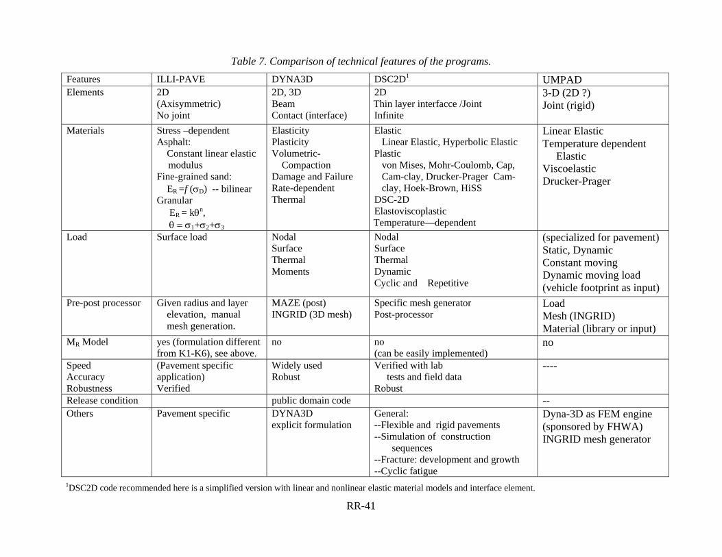
RR-41

Table 7. Comparison of technical features of the programs. Features ILLI-PAVE DYNA3D DSC2D1 UMPAD Elements 2D

(Axisymmetric) No joint

2D, 3D Beam Contact (interface)

2D Thin layer interfacce /Joint Infinite

3-D (2D ?) Joint (rigid)

Materials Stress –dependent Asphalt: Constant linear elastic

modulus Fine-grained sand: ER =f (σD) -- bilinear Granular ER = kθn, θ = σ1+σ2+σ3

Elasticity Plasticity Volumetric- Compaction Damage and Failure Rate-dependent Thermal

Elastic Linear Elastic, Hyperbolic Elastic Plastic von Mises, Mohr-Coulomb, Cap, Cam-clay, Drucker-Prager Cam- clay, Hoek-Brown, HiSS DSC-2D Elastoviscoplastic Temperature—dependent

Linear Elastic Temperature dependent Elastic Viscoelastic Drucker-Prager

Load Surface load Nodal Surface Thermal Moments

Nodal Surface Thermal Dynamic Cyclic and Repetitive

(specialized for pavement) Static, Dynamic Constant moving Dynamic moving load (vehicle footprint as input)

Pre-post processor Given radius and layer elevation, manual mesh generation.

MAZE (post) INGRID (3D mesh)

Specific mesh generator Post-processor

Load Mesh (INGRID) Material (library or input)

MR Model yes (formulation different from K1-K6), see above.

no no (can be easily implemented)

no

Speed Accuracy Robustness

(Pavement specific application) Verified

Widely used Robust

Verified with lab tests and field data Robust

----

Release condition public domain code -- Others Pavement specific

DYNA3D explicit formulation

General: --Flexible and rigid pavements --Simulation of construction sequences --Fracture: development and growth --Cyclic fatigue

Dyna-3D as FEM engine (sponsored by FHWA) INGRID mesh generator

1DSC2D code recommended here is a simplified version with linear and nonlinear elastic material models and interface element.

42

2.3 Final Selection

Table 8 summarizes the evaluations of each candidate program against the key efficiency and operational issues described earlier in this report. None of the programs has all of the technical and operational features desired for the flexible pavement response model. All of the programs can, with appropriate modifications, analyze the types of flexible pavement design scenarios to be considered in the 2002 Design Guide. Clearly, though, some programs will require more modification than others, and some of the modified codes will be more effective and efficient than others within the context of the 2002 Design Guide procedures. Based on the arguments outlined in this section, the flexible pavement analysis team adopted the DSC2D finite element program for the pavement response model. This decision was in part based on a process of elimination. ILLI-PAVE, although the only finite element program that already incorporates the stress dependent MR formulation to be used in the 2002 Design Guide, lacks many other key features, including infinite boundary elements, interface elements, and an efficient equation solver. DYNA3D, with its three-dimensional dynamic explicit formulation, is far more complex than is required for the purposes of the 2002 Design Guide; it also lacks infinite boundary elements, the appropriate nonlinear material model, and compatibility with a PC/Windows computing platform. UMPAD, which includes DYNA3D as one of its computation engines, rectifies some of the deficiencies in DYNA3D, specifically the lack of infinite boundary elements and, to some extent, compatibility with a PC/Windows computing platform. It also provides the NIKE3D implicit formulation as an alternative computation engine. However, UMPAD suffers from the same “overcomplexity” drawbacks as DYNA3D, and its key enhancement--the pavement-oriented pre- and post-processing system--is not especially useful for the 2002 Design Guide, as it would be replaced by the 2002 Design Guide user interface. The DSC2D program is not without its own deficiencies, specifically the lack of an infinite element and the appropriate stress-dependent material model. However, these deficiencies can be remedied relatively easily: • Implementation of infinite boundary elements. The formulation for these elements is

available in a later, more powerful version of the program (DSC-SST2D). This feature can thus be easily incorporated into the version to be used in the 2002 Design Guide.

• Implementation of the appropriate stress-dependent MR material model. The DSC-2D program already includes a hypoelastic nonlinear elasticity model, and this can be easily converted to the stress-dependent MR formulation.

A significant advantage to DSC2D is that Dr. C. Desai, the developer of the code, was a member of the project team, and he has an intimate knowledge of the algorithms and features implemented in the DSC2D code.

43

DSC2D has the additional operational drawback of not being a truly public domain program. Licensing issues are nonetheless expected to be very minor here. Dr. Desai agreed to make DSC2D available to NCHRP at no cost with only the following minimal conditions: 1. C.S. Desai will retain rights to continued use and distribution of the DSC2D program.

2. NCHRP can distribute the code only as part of the 2002 Design Guide software.

3. The following acknowledgment will be included in the 2002 Design Guide report and

software and transmitted to all who receive the software: “The DSC2D code was developed by C. Desai, Tucson, AZ. He has also developed enhanced general two- and three-dimensional DSC codes with many additional features such as: a wide selection of material models (elastic, plastic, HISS, creep, disturbance/damage, microcracking and fracture, fatigue life); static, dynamic, and repetitive loading; coupled fluid effects and thermal loading. For further information, contact: DSC, P.O. Box 65587, Tucson, AZ 85728, USA or e-mail csdesai@engr.arizona.edu.”

Note that although Dr. Desai developed the initial version of the DSC2D code, it has been substantially modified and enhanced for the 2002 Design Guide implementation.

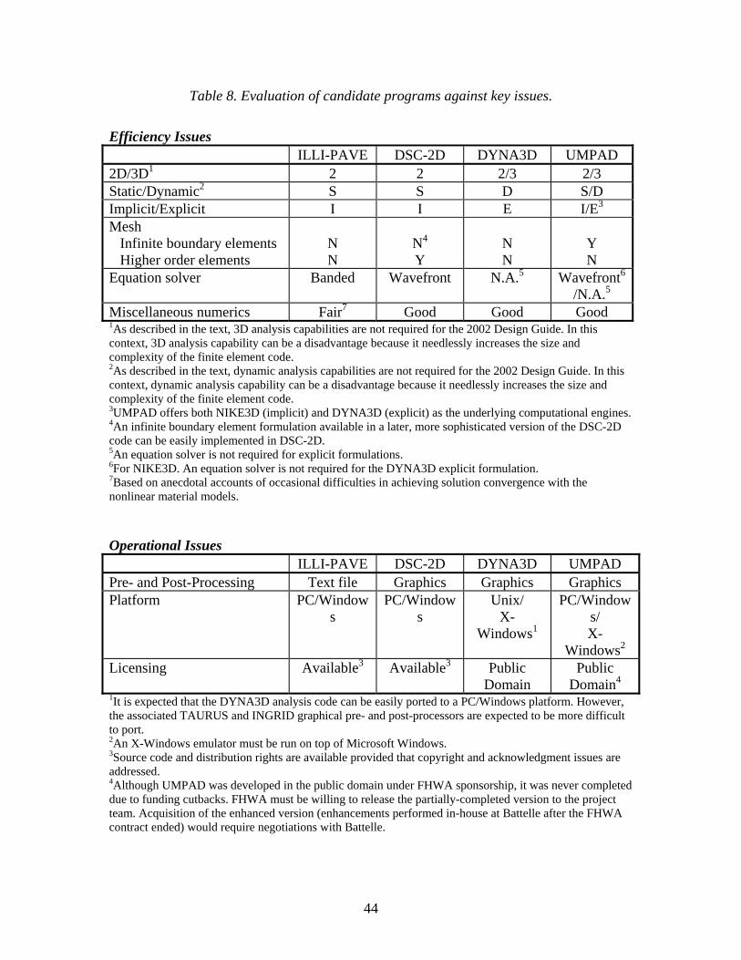
44

Table 8. Evaluation of candidate programs against key issues.

Efficiency Issues

ILLI-PAVE DSC-2D DYNA3D UMPAD 2D/3D1 2 2 2/3 2/3 Static/Dynamic2 S S D S/D Implicit/Explicit I I E I/E3

Mesh Infinite boundary elements Higher order elements

N N

N4

Y

N N

Y N

Equation solver Banded Wavefront N.A.5 Wavefront6

/N.A.5

Miscellaneous numerics Fair7 Good Good Good 1As described in the text, 3D analysis capabilities are not required for the 2002 Design Guide. In this context, 3D analysis capability can be a disadvantage because it needlessly increases the size and complexity of the finite element code. 2As described in the text, dynamic analysis capabilities are not required for the 2002 Design Guide. In this context, dynamic analysis capability can be a disadvantage because it needlessly increases the size and complexity of the finite element code. 3UMPAD offers both NIKE3D (implicit) and DYNA3D (explicit) as the underlying computational engines. 4An infinite boundary element formulation available in a later, more sophisticated version of the DSC-2D code can be easily implemented in DSC-2D. 5An equation solver is not required for explicit formulations. 6For NIKE3D. An equation solver is not required for the DYNA3D explicit formulation. 7Based on anecdotal accounts of occasional difficulties in achieving solution convergence with the nonlinear material models. Operational Issues

ILLI-PAVE DSC-2D DYNA3D UMPAD Pre- and Post-Processing Text file Graphics Graphics Graphics Platform PC/Window

s PC/Window

s Unix/

X-Windows1

PC/Windows/ X-

Windows2

Licensing Available3 Available3 Public Domain

Public Domain4

1It is expected that the DYNA3D analysis code can be easily ported to a PC/Windows platform. However, the associated TAURUS and INGRID graphical pre- and post-processors are expected to be more difficult to port. 2An X-Windows emulator must be run on top of Microsoft Windows. 3Source code and distribution rights are available provided that copyright and acknowledgment issues are addressed. 4Although UMPAD was developed in the public domain under FHWA sponsorship, it was never completed due to funding cutbacks. FHWA must be willing to release the partially-completed version to the project team. Acquisition of the enhanced version (enhancements performed in-house at Battelle after the FHWA contract ended) would require negotiations with Battelle.

45

3. ORGANIZATION OF THE FINITE ELEMENT PROGRAMS

The 2001 Design Guide finite element analysis procedure consists of three separate programs: PRE-DSC, DSC2D, and POST-DSC. All three programs are written in Fortran and have been compiled and linked using Compaq Visual Fortran V6.1. PRE-DSC is the pre-processor program for converting analysis control information generated by the 2002 Design Guide user interface program into an appropriate format for input to the DSC2D finite element analysis program. PRE-DSC contains the finite element mesh generator for modeling the layered pavement structure, loads, and boundary conditions. DSC2D is the finite element analysis program for determining stresses, strains, and displacements in nonlinear pavements systems. DSC2D is based upon a finite element code originally developed by C.S. Desai at the University of Arizona--Tucson, although it has been modified substantially for implementation within the 2002 Design Guide. Key features of DSC2D for the purposes of the 2002 Design Guide include:

• Axisymmetric nonlinear analysis formulation • Stress dependent resilient modulus model for unbound pavement layers • Full-slip, no-slip, and intermediate interface conditions between layers • Infinite boundary elements for reducing total analysis model size

POST-DSC is the post-processor program for converting the stress and strain data output from the DSC2D finite element analysis into an appropriate format for return back to the 2002 Design Guide user interface program, where it is used for pavement damage and performance prediction. POST-DSC contains the logic for superimposing the single wheel solutions generated by DSC2D into the appropriate multi-wheel solutions for single, tandem, tridem, and quad axles. PRE-DSC and POST-DSC will also contain capabilities for analyzing user-defined wheel configurations. However, this capability is not yet implemented in the current version of the program. Figure 22 through Figure 27 summarize the program logic and data flows for the DSC2D finite element program and its associated pre- and post-processors. Figure 22 gives the highest level view, illustrating the logic flow among the four major program modules. The user enters the pavement structure, traffic, and other analysis input data into the 2002 Design Guide user interface program. These data are passed via files to the PRE-DSC preprocessor program, where they are used to construct other data files describing the finite element mesh and other inputs required by the DSC2D analysis program and the POST-DSC postprocessor. The finite element input data stream generated by PRE-DSC is then processed by the DSC2D analysis program, which performs the calculations and outputs to separate files the strains and stresses computed at the centroids of each finite element for each load level and analysis period. These strains and stresses are combined

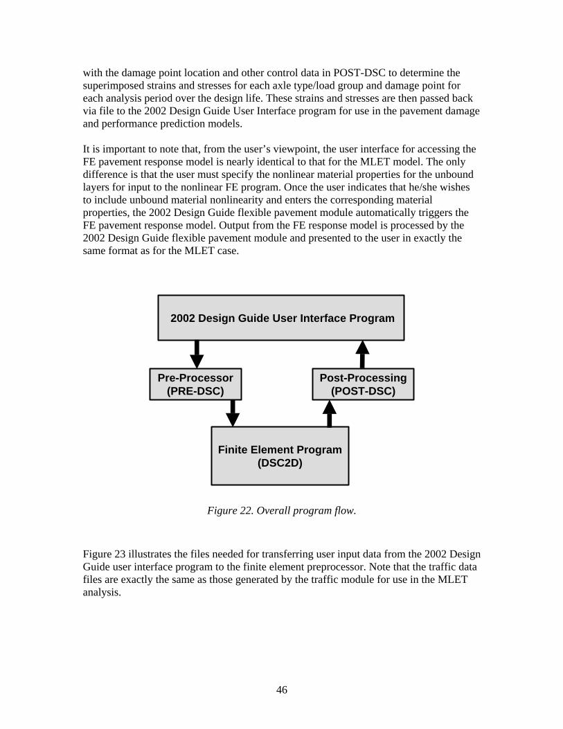
46

with the damage point location and other control data in POST-DSC to determine the superimposed strains and stresses for each axle type/load group and damage point for each analysis period over the design life. These strains and stresses are then passed back via file to the 2002 Design Guide User Interface program for use in the pavement damage and performance prediction models. It is important to note that, from the user’s viewpoint, the user interface for accessing the FE pavement response model is nearly identical to that for the MLET model. The only difference is that the user must specify the nonlinear material properties for the unbound layers for input to the nonlinear FE program. Once the user indicates that he/she wishes to include unbound material nonlinearity and enters the corresponding material properties, the 2002 Design Guide flexible pavement module automatically triggers the FE pavement response model. Output from the FE response model is processed by the 2002 Design Guide flexible pavement module and presented to the user in exactly the same format as for the MLET case.

2002 Design Guide User Interface Program

Pre-Processor(PRE-DSC)

Finite Element Program(DSC2D)

Post-Processing(POST-DSC)

Figure 22. Overall program flow.

Figure 23 illustrates the files needed for transferring user input data from the 2002 Design Guide user interface program to the finite element preprocessor. Note that the traffic data files are exactly the same as those generated by the traffic module for use in the MLET analysis.

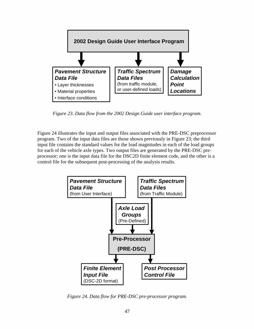
47

2002 Design Guide User Interface Program

Pavement StructureData File• Layer thicknesses• Material properties• Interface conditions

Traffic SpectrumData Files(from traffic module, or user-defined loads)

DamageCalculationPoint Locations

Figure 23. Data flow from the 2002 Design Guide user interface program.

Figure 24 illustrates the input and output files associated with the PRE-DSC preprocessor program. Two of the input data files are those shown previously in Figure 23; the third input file contains the standard values for the load magnitudes in each of the load groups for each of the vehicle axle types. Two output files are generated by the PRE-DSC pre-processor; one is the input data file for the DSC2D finite element code, and the other is a control file for the subsequent post-processing of the analysis results.

Pre-Processor

(PRE-DSC)

Pavement StructureData File(from User Interface)

Traffic SpectrumData Files(from Traffic Module)

Finite ElementInput File(DSC-2D format)

Post ProcessorControl File

Axle Load Groups

(Pre-Defined)

Figure 24. Data flow for PRE-DSC pre-processor program.

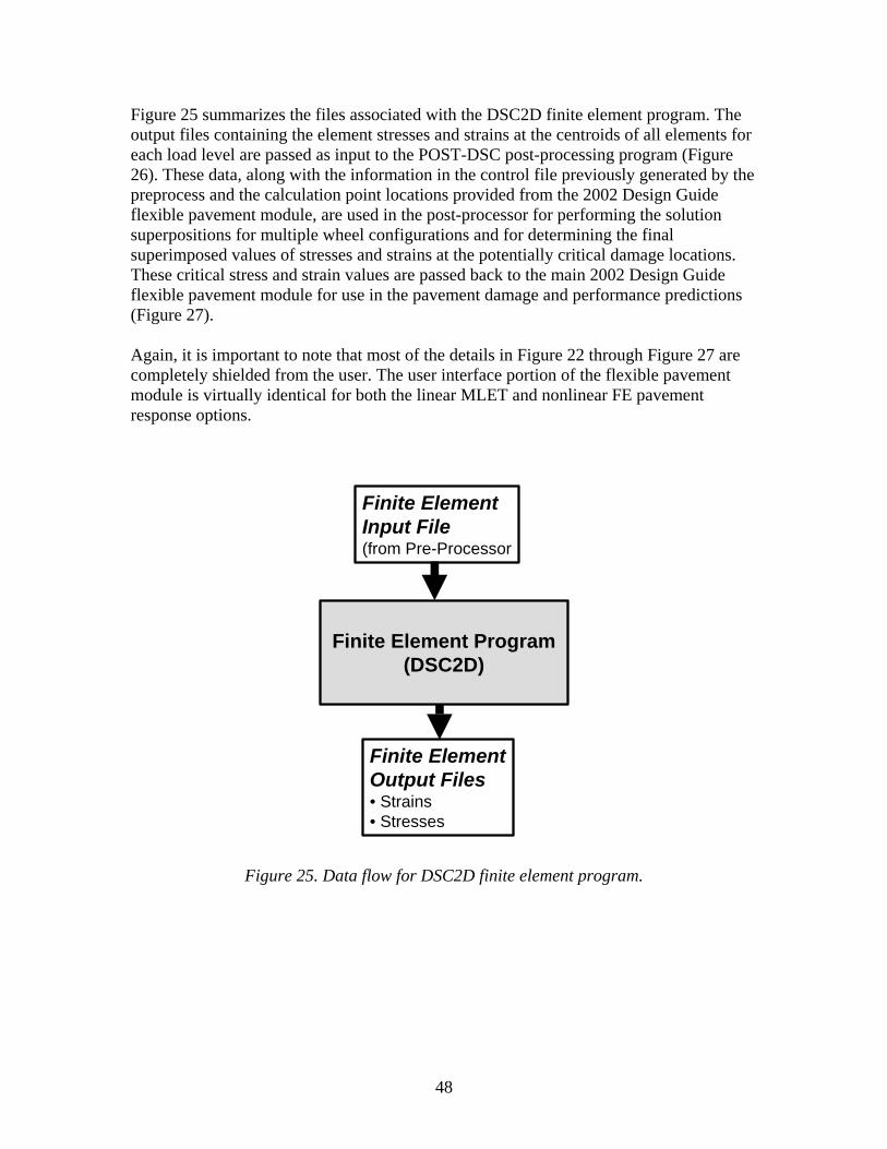
48

Figure 25 summarizes the files associated with the DSC2D finite element program. The output files containing the element stresses and strains at the centroids of all elements for each load level are passed as input to the POST-DSC post-processing program (Figure 26). These data, along with the information in the control file previously generated by the preprocess and the calculation point locations provided from the 2002 Design Guide flexible pavement module, are used in the post-processor for performing the solution superpositions for multiple wheel configurations and for determining the final superimposed values of stresses and strains at the potentially critical damage locations. These critical stress and strain values are passed back to the main 2002 Design Guide flexible pavement module for use in the pavement damage and performance predictions (Figure 27). Again, it is important to note that most of the details in Figure 22 through Figure 27 are completely shielded from the user. The user interface portion of the flexible pavement module is virtually identical for both the linear MLET and nonlinear FE pavement response options.

Finite Element Program(DSC2D)

Finite ElementInput File(from Pre-Processor

Finite ElementOutput Files• Strains• Stresses

Figure 25. Data flow for DSC2D finite element program.

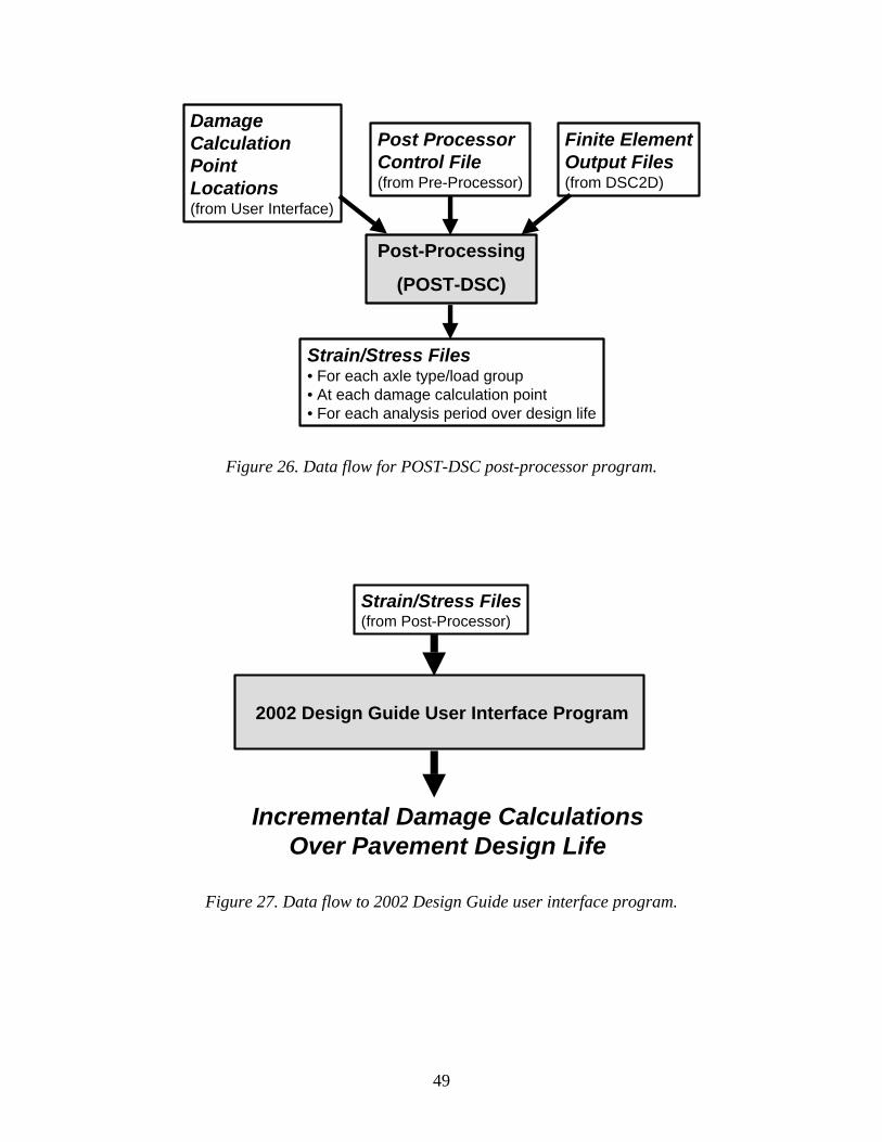
49

Post-Processing

(POST-DSC)

Post ProcessorControl File(from Pre-Processor)

Finite ElementOutput Files(from DSC2D)

DamageCalculationPoint Locations(from User Interface)

Strain/Stress Files• For each axle type/load group• At each damage calculation point• For each analysis period over design life

Figure 26. Data flow for POST-DSC post-processor program.

2002 Design Guide User Interface Program

Strain/Stress Files(from Post-Processor)

Incremental Damage CalculationsOver Pavement Design Life

Figure 27. Data flow to 2002 Design Guide user interface program.

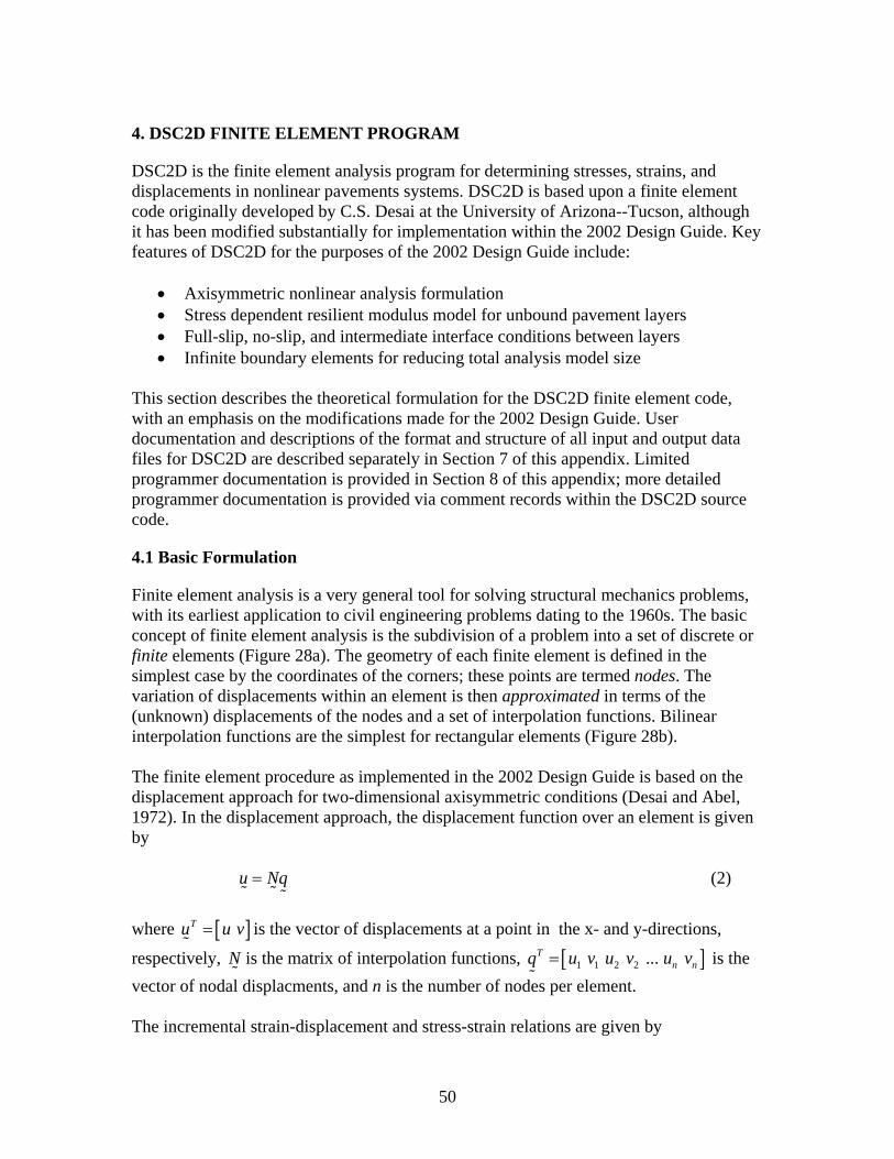
50

4. DSC2D FINITE ELEMENT PROGRAM

DSC2D is the finite element analysis program for determining stresses, strains, and displacements in nonlinear pavements systems. DSC2D is based upon a finite element code originally developed by C.S. Desai at the University of Arizona--Tucson, although it has been modified substantially for implementation within the 2002 Design Guide. Key features of DSC2D for the purposes of the 2002 Design Guide include:

• Axisymmetric nonlinear analysis formulation • Stress dependent resilient modulus model for unbound pavement layers • Full-slip, no-slip, and intermediate interface conditions between layers • Infinite boundary elements for reducing total analysis model size

This section describes the theoretical formulation for the DSC2D finite element code, with an emphasis on the modifications made for the 2002 Design Guide. User documentation and descriptions of the format and structure of all input and output data files for DSC2D are described separately in Section 7 of this appendix. Limited programmer documentation is provided in Section 8 of this appendix; more detailed programmer documentation is provided via comment records within the DSC2D source code.

4.1 Basic Formulation

Finite element analysis is a very general tool for solving structural mechanics problems, with its earliest application to civil engineering problems dating to the 1960s. The basic concept of finite element analysis is the subdivision of a problem into a set of discrete or finite elements (Figure 28a). The geometry of each finite element is defined in the simplest case by the coordinates of the corners; these points are termed nodes. The variation of displacements within an element is then approximated in terms of the (unknown) displacements of the nodes and a set of interpolation functions. Bilinear interpolation functions are the simplest for rectangular elements (Figure 28b). The finite element procedure as implemented in the 2002 Design Guide is based on the displacement approach for two-dimensional axisymmetric conditions (Desai and Abel, 1972). In the displacement approach, the displacement function over an element is given by u Nq=

% % % (2)

where [ ] Tu u v=

%is the vector of displacements at a point in the x- and y-directions,

respectively, N%

is the matrix of interpolation functions, [ ]1 1 2 2 ... Tn nq u v u v u v=

% is the

vector of nodal displacments, and n is the number of nodes per element. The incremental strain-displacement and stress-strain relations are given by

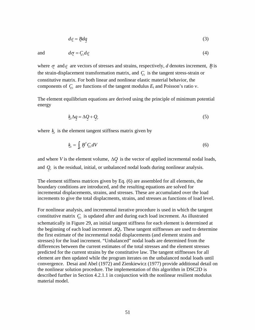
51

d Bdqε =

%% % (3)

and td C dσ ε=

% % % (4)

where σ

% andε

% are vectors of stresses and strains, respectively, d denotes increment, B

%is

the strain-displacement transformation matrix, and tC%

is the tangent stress-strain or constitutive matrix. For both linear and nonlinear elastic material behavior, the components of tC

% are functions of the tangent modulus Et and Poisson’s ratio ν.

The element equilibrium equations are derived using the principle of minimum potential energy t rk q Q Q∆ = ∆ +

% % % % (5)

where tk

% is the element tangent stiffness matrix given by

T

t tVk B C dV= ∫ %% %

(6)

and where V is the element volume, Q∆

% is the vector of applied incremental nodal loads,

and rQ%

is the residual, initial, or unbalanced nodal loads during nonlinear analysis. The element stiffness matrices given by Eq. (6) are assembled for all elements, the boundary conditions are introduced, and the resulting equations are solved for incremental displacements, strains, and stresses. These are accumulated over the load increments to give the total displacments, strains, and stresses as functions of load level. For nonlinear analysis, and incremental iterative procedure is used in which the tangent constitutive matrix tC

% is updated after and during each load increment. As illustrated

schematically in Figure 29, an initial tangent stiffness for each element is determined at the beginning of each load increment ∆Qi. These tangent stiffnesses are used to determine the first estimate of the incremental nodal displacements (and element strains and stresses) for the load increment. “Unbalanced” nodal loads are determined from the differences between the current estimates of the total stresses and the element stresses predicted for the current strains by the constitutive law. The tangent stiffnesses for all element are then updated while the program iterates on the unbalanced nodal loads until convergence. Desai and Abel (1972) and Zienkiewicz (1977) provide additional detail on the nonlinear solution procedure. The implementation of this algorithm in DSC2D is described further in Section 4.2.1.1 in conjunction with the nonlinear resilient modulus material model.

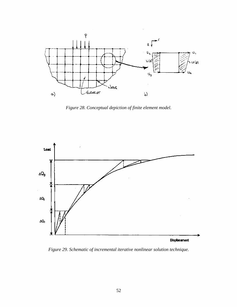
52

Figure 28. Conceptual depiction of finite element model.

Figure 29. Schematic of incremental iterative nonlinear solution technique.

53

4.2 Nonlinear Resilient Modulus Model

The resilient modulus, defined as the unloading modulus after many cycles of repeated loading, is used in pavement engineering as an appropriate measure of stiffness for the unbound (i.e., soil) layers in a pavement structure. The definition of the resilient modulus as measured in the standard resilient modulus cyclic triaxial test is shown in Figure 30 in which σa and εa are the stress and strain in the axial (i.e., cyclic loading) direction. The sample is initially subjected to a hydrostatic confining pressure σc, which induces an initial strain εc (unmeasured in the test, but the same in all directions for isotropic material behavior). The axial stress is then cycled at a constant magnitude ∆σ, which induces the cyclic resilient axial strain ∆ε. The resilient modulus MR is defined simply as the ratio of the cyclic axial stress to resilient axial strain:

RM σε

∆=

∆ (7)

The resilient modulus for most unbound pavement materials is stress dependent. Many nonlinear models have been proposed over the years for incorporating the effects of stress level on the resilient modulus. A general form for these models can be expressed as (Andrei, 1999):

2 3

61 7

3k k

octR a

a a

kM k p kp p

θ τ⎛ ⎞ ⎛ ⎞−= +⎜ ⎟ ⎜ ⎟

⎝ ⎠ ⎝ ⎠ (8)

in which MR = resilient modulus

θ = bulk stress at the peak of the loading = σx + σy + σz = 3σc + ∆σ for standard triaxial compression loading

τoct = octahedral shear stress at the peak of the loading

= ( ) ( ) ( )1/ 2

2 2 2 2 2 21 29 3x y y z z x xy yz zxσ σ σ σ σ σ τ τ τ⎧ ⎫⎡ ⎤ ⎡ ⎤− + − + − + + +⎨ ⎬⎣ ⎦⎢ ⎥⎣ ⎦⎩ ⎭

= 23

σ∆ for standard triaxial compression loading

pa = atmospheric pressure (normalizing factor) k1-k7 = material parameters subject to the following constraints: k1 > 0; k2 > 0; k3 < 0; k6 < 0; k7 > 1

A simplified version of Eq. (8) with k6=0 and k7=1 has been adopted for the 2002 Design Guide. Some typical values for pavement unbound materials as determined by Andrei (2001) are given in Table 9 and Table 10.

54

Equation (8) combines both the stiffening effect of bulk stress (the term under the k2 exponent) and the softening effect of shear stress (the term under the k3 exponent). Through appropriate choices of the material parameters k1-k7, one can recover the familiar two-parameter bulk stress model for granular materials and its companion two-parameter shear stress model for cohesive soils, the Uzan-Witczak “universal” model (Witczak and Uzan, 1988), and the k1-k6 model from the Strategic Highway Research Program’s (SHRP) flexible pavement performance models (Lytton et al., 1993).13 Equation (8) and its various specializations are convenient functional forms for fitting laboratory resilient modulus test data. However, they are less convenient—in fact, quite problematic—for implementation in a conventional incremental-implicit finite element framework: 1. The conventional definition of MR as shown in Figure 30 corresponds to neither a

tangent modulus or a secant modulus, but rather to a chord modulus. In terms of the axial stress vs. axial strain response for the conventional triaxial resilient modulus test, the resilient modulus is defined as the slope of the chord connecting the peak cyclic stress point (εc+∆ε, σc+∆σ) to the confining pressure point (εc, σc) on the unloading curve. Note that only the resilient strain increment ∆ε is measured during the test; the magnitude of the confining pressure strain εc is unknown.

2. The MR nonlinearity is defined in Eq. (8) in terms of stresses rather than strains. Contrast this, for example, with the conventional hypoelastic constitutive model defined in terms of strain invariants (see, e.g., Desai and Siriwardane, 1984). Conventional displacement-based incremental-implicit and explicit finite element algorithms take strains and strain increments as the fundamental solution quantities, so the stress-based formulation in Eq. (8) is inconvenient.

3. The MR model in Eq. (8) is defined exclusively in terms of stresses at the end of the loading path. For standard incremental-implicit and explicit finite element algorithms, it is usually more convenient to define stiffness at the beginning of the load increment.

4. There may be constraints on the material parameters k1-k7 in addition to the obvious physical requirements given in the definitions for the equation. Specifically, additional constraints (primarily between k2, k3, θ, and τoct) may be required to ensure that the tangent modulus is always positive for pre-peak failure conditions and to ensure solution uniqueness.

Point 3 merits additional discussion. Within the narrow context of the conventional triaxial compression resilient modulus test in which the initial hydrostatic confining stress

13 In fact, the historical precedent of the SHRP performance models, which used material parameters k4 and k5 for the stress dependent Poisson’s ratio, is the reason that these two material parameters are absent in Eq. (83).

55

isheld constant and only the axial stress is cycled, the peak stresses are related to the initial stresses as follows:

3 cθ σ σ= + ∆ (9)

23octτ σ= ∆ (10)

Equations (9) and (10) define an implicit relationship among θ, τoct, and σc:

3 2

octc

τθσ = − (11)

Thus, in the standard triaxial resilient modulus test there is a one-to-one correspondence between the stress state θ, τoct at the peak of the cyclic loading and the cylic loading stresses σc, ∆σc. In other words, the standard test provides only one load path to reach each peak θ, τoct combination. However, Eq. (8) is intended for general use in analyzing the more complex stress states in real pavement structures. The question of how well this conforms to the real behavior of unbound material in the general case requires further study. Past implementation of stress-dependent resilient moduli models for unbound pavement materials have most commonly employed an iterative secant approach. This approach has been found to exhibit convergence difficulties in many cases (see, e.g., Brown and Pappin, 1981; Tutumluer, 1995). In addition, it is not suitable for explicit finite element formulations. Hjelmstad and Taciroglu (2001) provide an elegant derivation of the simpler Uzan-Witczak stress-dependent resilient modulus model in tangent modulus form that addresses issues 2 and 3 above but which does not recognize the complications of issue 1.

56

RM σε

∆=

∆

εc

σc

∆ε

∆σ MR

εa

σa

Figure 30. Definition of resilient modulus as a chord modulus.

Soil ID Project/Study Description AASHTO Unifiedclassification classification

S12 MnRoad Class 6 base A-1-a SW-SMS1 USACE-CRREL Silty sand from Moulton Pit A-4(1) SMS3 USACE-CRREL Clay from St. Albans A-6(9) CLS11 MnRoad Class 3 subbase A-1-b SMS7 ALF-FHWA ALF subgrade A-4(3) SMS13 MnRoad Silty sand subgrade A-6(7) CL

Table 9. Soil types tested by Andrei (2001).

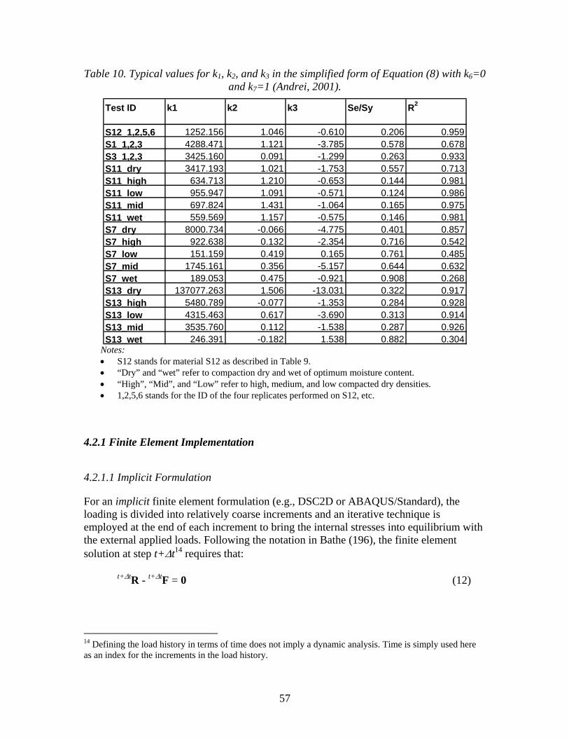
57

Table 10. Typical values for k1, k2, and k3 in the simplified form of Equation (8) with k6=0 and k7=1 (Andrei, 2001).

Test ID k1 k2 k3 Se/Sy R2

S12_1,2,5,6 1252.156 1.046 -0.610 0.206 0.959S1_1,2,3 4288.471 1.121 -3.785 0.578 0.678S3_1,2,3 3425.160 0.091 -1.299 0.263 0.933S11_dry 3417.193 1.021 -1.753 0.557 0.713S11_high 634.713 1.210 -0.653 0.144 0.981S11_low 955.947 1.091 -0.571 0.124 0.986S11_mid 697.824 1.431 -1.064 0.165 0.975S11_wet 559.569 1.157 -0.575 0.146 0.981S7_dry 8000.734 -0.066 -4.775 0.401 0.857S7_high 922.638 0.132 -2.354 0.716 0.542S7_low 151.159 0.419 0.165 0.761 0.485S7_mid 1745.161 0.356 -5.157 0.644 0.632S7_wet 189.053 0.475 -0.921 0.908 0.268S13_dry 137077.263 1.506 -13.031 0.322 0.917S13_high 5480.789 -0.077 -1.353 0.284 0.928S13_low 4315.463 0.617 -3.690 0.313 0.914S13_mid 3535.760 0.112 -1.538 0.287 0.926S13_wet 246.391 -0.182 1.538 0.882 0.304

Notes: • S12 stands for material S12 as described in Table 9. • “Dry” and “wet” refer to compaction dry and wet of optimum moisture content. • “High”, “Mid”, and “Low” refer to high, medium, and low compacted dry densities. • 1,2,5,6 stands for the ID of the four replicates performed on S12, etc.

4.2.1 Finite Element Implementation

4.2.1.1 Implicit Formulation

For an implicit finite element formulation (e.g., DSC2D or ABAQUS/Standard), the loading is divided into relatively coarse increments and an iterative technique is employed at the end of each increment to bring the internal stresses into equilibrium with the external applied loads. Following the notation in Bathe (196), the finite element solution at step t+∆t14 requires that: t+∆tR - t+∆tF = 0 (12)

14 Defining the load history in terms of time does not imply a dynamic analysis. Time is simply used here as an index for the increments in the load history.

58

in which bold fonts indicate vector or matrix quantities, t+∆tR is the vector of applied nodal loads at step t+∆t, and t+∆tF is the vector of equivalent nodal loads corresponding to the internal element stresses. Note that t+∆tR is derived from the prescribed loading history and therefore is known at all steps in the analysis. Equation (12) simply states that the internal element stresses must be in equilibrium with the applied loads at step t+∆t. Since the solution is known at step t: t+∆tF = tF + F (13) in which F is the increment in nodal forces corresponding to the increment in element stresses from step t to step t+∆t. F can be approximated using the tangent stiffness matrix tK, which is based on the tangent elastic constants at step t: F ≅ tK U (14) in which U is the vector of incremental nodal displacements between t and t+∆t. The tangent stiffness matrix tK is expressed as: ( ) )()()()(

)(

mm

m V

mtTmt dVm

BCBK ∑ ∫= (15)

in which the superscript m designates element m, V(m) is the volume of element m, B(m) is the strain-displacement interpolation matrix, B(m)T is the transpose of B(m), and tC(m) is the tangent constitutive matrix for element m at step t, e.g.:

( )( )( )

( )

( )( )

( )⎥⎥⎥⎥⎥⎥⎥

⎦

⎤

⎢⎢⎢⎢⎢⎢⎢

⎣

⎡

−−

−

−

−+−

=

)(

)(

)(

)(

)(

)(

)()(

)()()(

122100

011

01

1

2111

mT

t

mT

t

mT

t

mT

t

mT

t

mT

t

mT

tmT

t

mT

tmT

tmt E

νν

νν

νν

ννν

C (16)

for plane strain conditions, in which tET

(m) and tνT(m) are the tangent elastic properties at

step t for element m. Combining Eqs. (12), (13), and (14) gives: tK U ≅ t+∆tR - tF (17) Solving for U, we can calculate an approximation to the displacements at step t+∆t: t+∆tU ≅ tU + U (18)

59

This solution is approximate because the calculations are based on the tangent stiffness matrix tK at step t (Eq. (14)). The error in this approximation will become diminishingly small as the step size ∆t approaches zero. However, for the relatively large step sizes commonly used with the implicit formulation, the errors may be quite large and an iterative correction scheme is warranted. This correction is typically based upon Newton-Raphson iteration of Eqs. (17) and (18): t+∆tK(i-1) ∆U(i) = t+∆tR – t+∆tF(i-1) (19) t+∆tU(i) = t+∆tU(i-1) + ∆U(i) (20) with the initial conditions t+∆tU(0) = tU, t+∆tK(0) = tK, and t+∆tF(0) = tF. In Eqs. (19) and (20), i designates the iteration cycle; t+∆tR – t+∆tF(i-1) represents the out-of-balance load vector—i.e., the loads that are not yet balanced by element stresses, and ∆U(i) represents the additional incremental nodal displacements required to bring the element stresses into equilibrium. Note that in practical terms it may not be computationally effective to reform the tangent stiffness matrix at each iteration cycle in Eq. (19). Instead, the iterations can be performed with the already-computed tangent stiffness matrix tK (Eq. (15)); this, of course, will tend to increase the number of iterations required for convergence in each step. DSC2D does update the tangent stiffness matrix at each iteration cycle as indicated by Eq. (19). The element strains and stresses are also computed during the equilibrium iteration process as: ∆ε(m)(i) = B(m) ∆U(i) (21) t+∆tε(m)(i) = t+∆tε(m)(i-1) + ∆ε(m)(i) (22) t+∆tσ(m)(i) = t+∆tσ(m)(i-1) + t+∆tC(m)(i-1) ∆ε(m)(i) (23) with the initial conditions t+∆tε(m)(0) = tε(m), t+∆tσ(m)(0) = tσ(m), and t+∆tC(m)(0) = tC(m). For consistency, if the iterations are performed with a constant tangent stiffness matrix tK, then the iterations in Eqs. (21) through (23) should be performed with a constant tangent stiffness constitutive matrix tC(m) (eq. Eq. (16)).

4.2.1.2 Tangent Elastic Modulus

The generalized form of Hooke’s law for a nonlinearly elastic material under conventional triaxial compression loading is:

[ ] ( )1 1 12 1 2a a c s c cs s sE E E

= − = + − = +⎡ ⎤⎣ ⎦ε σ νσ ∆σ ν σ ∆σ ε (24)

in which Es and νs are the secant Young’s modulus and Poisson’s ratio and

60

( )1 1 2c c ssE

= −ε σ ν (25) is the initial strain due to the confining pressure (not measured in test). Note that the standard resilient modulus test provides no insight into the secant Poisson’s ratio νs in Eq.(24); typically, an assumed value is used for this parameter. Equation (24) can be expressed in terms of the resilient modulus MR as (see Figure 30):

1a c

RM= +ε ∆σ ε (26)

The tangent Young’s modulus ET required for conventional incremental finite element formulations can be derived from the secant Young’s modulus ES as15:

( )0

lim a ST S a a S

a a a

d dEdE E Ed d d∆ →

∆= = = = +

∆ε

σσ ε εε ε ε ε

(27)

or in terms of MR as:

( ) RT R a a R

a a

d dME M Md d

= = +ε εε ε

(28)

Since MR is defined in terms of stresses rather than strains, it is more convenient to formulate the derivation in terms of the tangent and secant elastic compliances DT=(ET)-1 and DS=(ES)-1=(MR)-1, respectively. Equation (28) can be expressed in terms of compliances as:

( )0

lim a ST S a a S

a a a

d dDdD D Dd d d∆ →

∆= = = = +

∆σ

εε σ σσ σ σ σ

(29)

From Eq. (8) the secant compliance DS can be expressed as:

15 An alternative to deriving ET is the total strain approach employed by Uzan in the SHRP performance models (Lytton et al., 1993), which in compliance terms can be expressed as:

x x x x x xx x y z xy yz zx

x y z xy yz zx

∂ ∂ ∂ ∂ ∂ ∂= + + + + +

∂ ∂ ∂ ∂ ∂ ∂& & & & & & &

ε ε ε ε ε εε σ σ σ τ τ τ

σ σ σ τ τ τ

in which , , i j ij& & &ε σ τ are the strain and stress increments. One consequence of this approach is a nonsymmetric compliance matrix. See the addendum at the end of this Appendix for more details.

61

2 3

1

11 1

k k

t oct

a aS

S R a

p pD

E M k p

− −⎛ ⎞ ⎛ ⎞+

+⎜ ⎟ ⎜ ⎟⎝ ⎠ ⎝ ⎠= = =

θ θ τ

(30)

and, using σa = σ1, the tangent compliance DT can be expressed as

2 3 2 3

11 1 1

1 1k k k k

t oct t oct

a a a aT

a a

p p p pdDd k p k p

− − − −⎡ ⎤⎛ ⎞ ⎛ ⎞ ⎛ ⎞ ⎛ ⎞+ ++ +⎢ ⎥⎜ ⎟ ⎜ ⎟ ⎜ ⎟ ⎜ ⎟

⎢ ⎥⎝ ⎠ ⎝ ⎠ ⎝ ⎠ ⎝ ⎠= +⎢ ⎥⎢ ⎥⎢ ⎥⎣ ⎦

θ θ τ θ θ τ

σσ

(31)

or

2 3 2 3

2 3

1 1

2 3

12 21 1

1

21 13

1

k k k k

t oct t oct

a a a aT

a a

k k

t oct

a a

a

k kp p p p

Dk p k p

p pk p

− − − − − −

− −

⎡ ⎤⎛ ⎞ ⎛ ⎞ ⎛ ⎞ ⎛ ⎞+ +− + − +⎢ ⎥⎜ ⎟ ⎜ ⎟ ⎜ ⎟ ⎜ ⎟

⎢ ⎥⎝ ⎠ ⎝ ⎠ ⎝ ⎠ ⎝ ⎠= +⎢ ⎥⎢ ⎥⎢ ⎥⎣ ⎦

⎛ ⎞ ⎛ ⎞++⎜ ⎟ ⎜ ⎟

⎝ ⎠ ⎝ ⎠+

θ θ τ θ θ τ

σ

θ θ τ

(32)

Typical variations of ES and ET with strain for various k2 and k3 values as determined using this formulation are illustrated in .

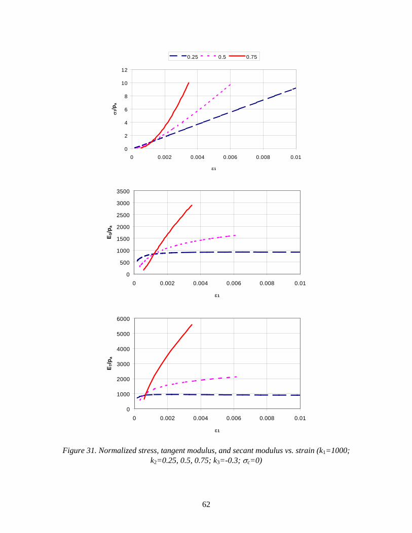
62

0

2

4

6

8

10

12

0 0.002 0.004 0.006 0.008 0.01

ε1

σ1/p

a

0.25 0.5 0.75

0

500

1000

1500

2000

2500

3000

3500

0 0.002 0.004 0.006 0.008 0.01

ε1

E S/p

a

0

1000

2000

3000

4000

5000

6000

0 0.002 0.004 0.006 0.008 0.01

ε1

E T/p

a

Figure 31. Normalized stress, tangent modulus, and secant modulus vs. strain (k1=1000;

k2=0.25, 0.5, 0.75; k3=-0.3; σc=0)

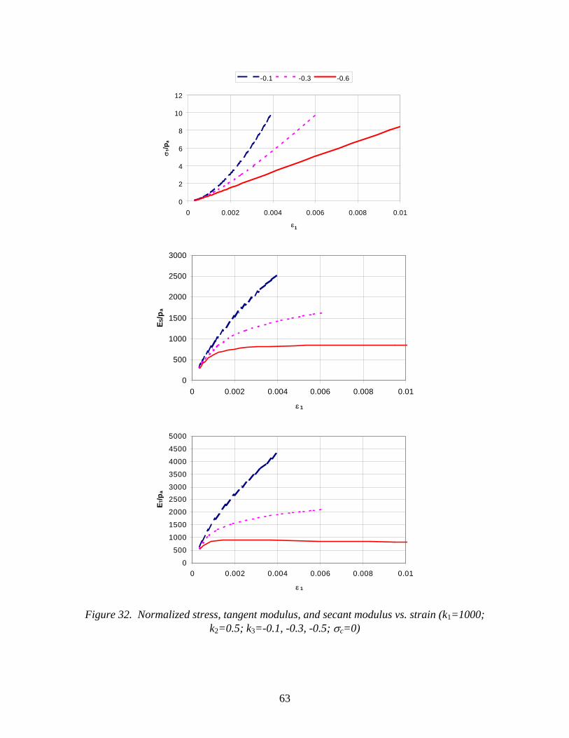
63

0

2

4

6

8

10

12

0 0.002 0.004 0.006 0.008 0.01

ε1

σ

-0.1 -0.3 -0.6

0

500

1000

1500

2000

2500

3000

0 0.002 0.004 0.006 0.008 0.01

ε 1

E S/p

a

0

500

1000

1500

2000

25003000

3500

4000

4500

5000

0 0.002 0.004 0.006 0.008 0.01

ε 1

E T/p

a

Figure 32. Normalized stress, tangent modulus, and secant modulus vs. strain (k1=1000;

k2=0.5; k3=-0.1, -0.3, -0.5; σc=0)

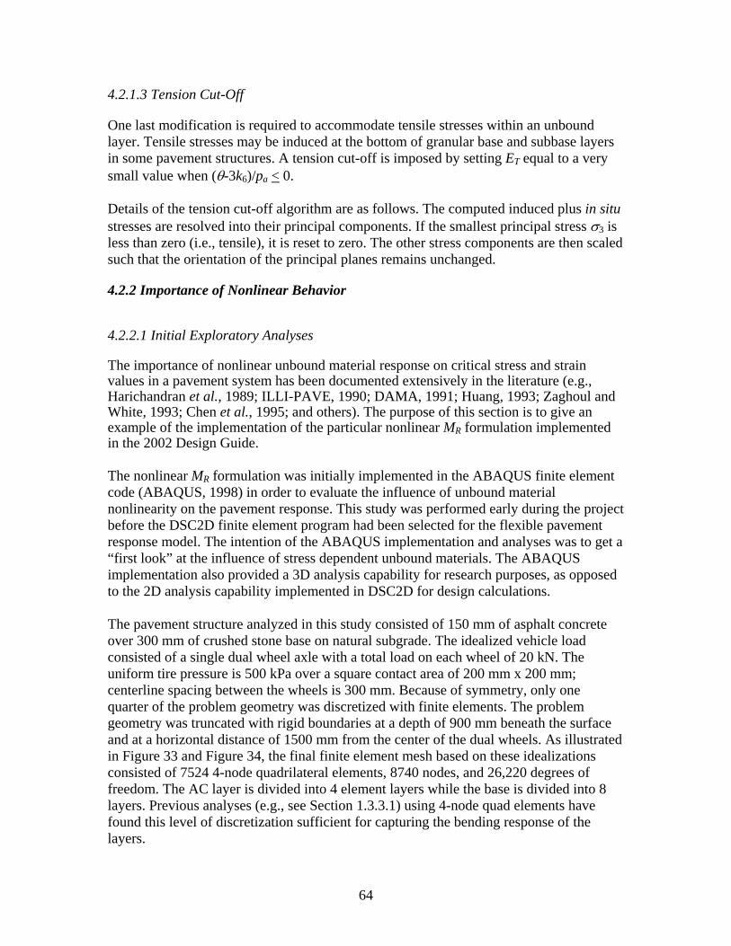
64

4.2.1.3 Tension Cut-Off

One last modification is required to accommodate tensile stresses within an unbound layer. Tensile stresses may be induced at the bottom of granular base and subbase layers in some pavement structures. A tension cut-off is imposed by setting ET equal to a very small value when (θ-3k6)/pa < 0. Details of the tension cut-off algorithm are as follows. The computed induced plus in situ stresses are resolved into their principal components. If the smallest principal stress σ3 is less than zero (i.e., tensile), it is reset to zero. The other stress components are then scaled such that the orientation of the principal planes remains unchanged.

4.2.2 Importance of Nonlinear Behavior

4.2.2.1 Initial Exploratory Analyses

The importance of nonlinear unbound material response on critical stress and strain values in a pavement system has been documented extensively in the literature (e.g., Harichandran et al., 1989; ILLI-PAVE, 1990; DAMA, 1991; Huang, 1993; Zaghoul and White, 1993; Chen et al., 1995; and others). The purpose of this section is to give an example of the implementation of the particular nonlinear MR formulation implemented in the 2002 Design Guide. The nonlinear MR formulation was initially implemented in the ABAQUS finite element code (ABAQUS, 1998) in order to evaluate the influence of unbound material nonlinearity on the pavement response. This study was performed early during the project before the DSC2D finite element program had been selected for the flexible pavement response model. The intention of the ABAQUS implementation and analyses was to get a “first look” at the influence of stress dependent unbound materials. The ABAQUS implementation also provided a 3D analysis capability for research purposes, as opposed to the 2D analysis capability implemented in DSC2D for design calculations. The pavement structure analyzed in this study consisted of 150 mm of asphalt concrete over 300 mm of crushed stone base on natural subgrade. The idealized vehicle load consisted of a single dual wheel axle with a total load on each wheel of 20 kN. The uniform tire pressure is 500 kPa over a square contact area of 200 mm x 200 mm; centerline spacing between the wheels is 300 mm. Because of symmetry, only one quarter of the problem geometry was discretized with finite elements. The problem geometry was truncated with rigid boundaries at a depth of 900 mm beneath the surface and at a horizontal distance of 1500 mm from the center of the dual wheels. As illustrated in Figure 33 and Figure 34, the final finite element mesh based on these idealizations consisted of 7524 4-node quadrilateral elements, 8740 nodes, and 26,220 degrees of freedom. The AC layer is divided into 4 element layers while the base is divided into 8 layers. Previous analyses (e.g., see Section 1.3.3.1) using 4-node quad elements have found this level of discretization sufficient for capturing the bending response of the layers.

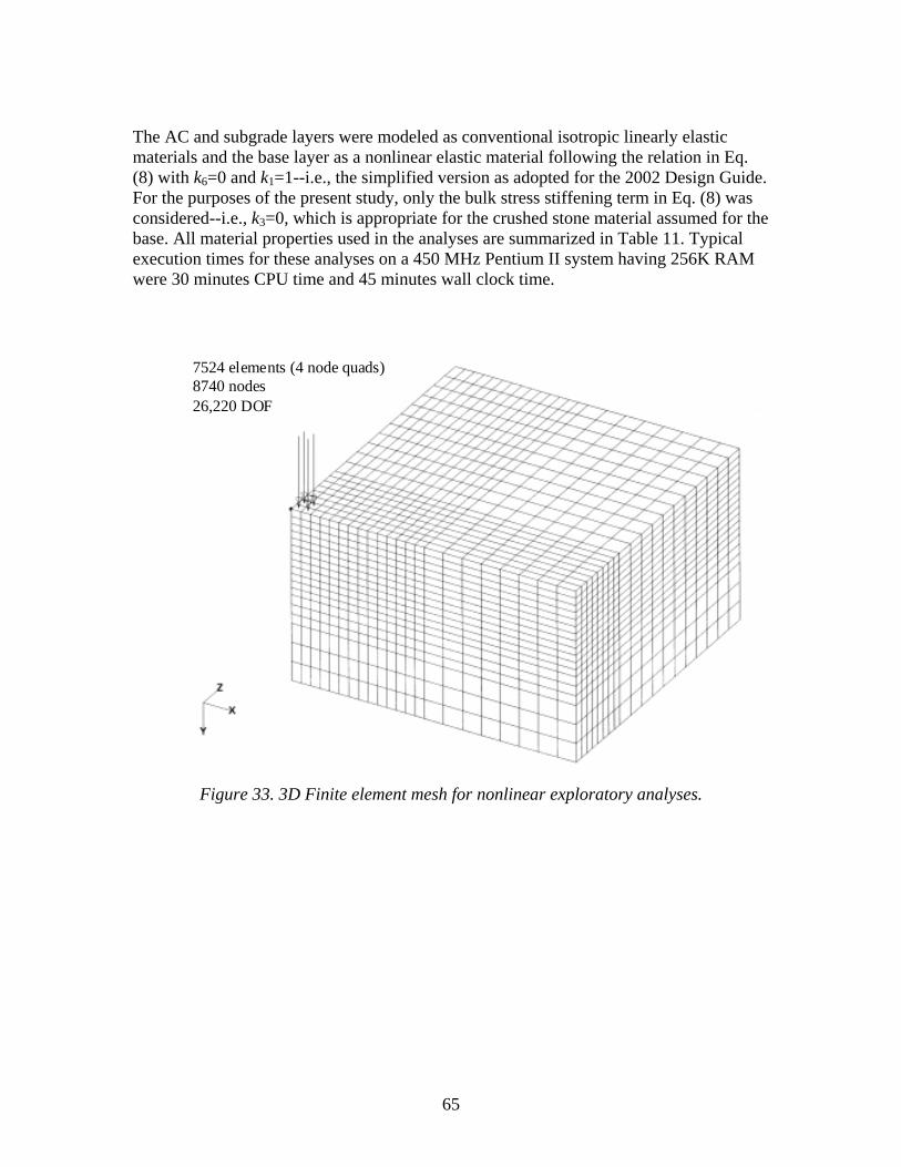
65

The AC and subgrade layers were modeled as conventional isotropic linearly elastic materials and the base layer as a nonlinear elastic material following the relation in Eq. (8) with k6=0 and k1=1--i.e., the simplified version as adopted for the 2002 Design Guide. For the purposes of the present study, only the bulk stress stiffening term in Eq. (8) was considered--i.e., k3=0, which is appropriate for the crushed stone material assumed for the base. All material properties used in the analyses are summarized in Table 11. Typical execution times for these analyses on a 450 MHz Pentium II system having 256K RAM were 30 minutes CPU time and 45 minutes wall clock time.

7524 elements (4 node quads)8740 nodes26,220 DOF

Figure 33. 3D Finite element mesh for nonlinear exploratory analyses.

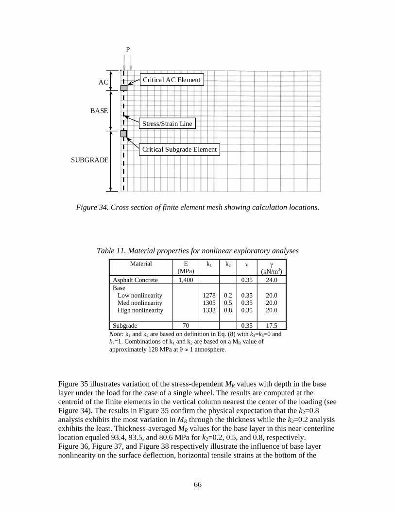
66

AC

BASE

SUBGRADE

P

Stress/Strain Line

Critical Subgrade Element

Critical AC Element

Figure 34. Cross section of finite element mesh showing calculation locations.

Table 11. Material properties for nonlinear exploratory analyses Material E

(MPa) k1 k2 ν γ

(kN/m3) Asphalt Concrete 1,400 0.35 24.0 Base Low nonlinearity Med nonlinearity High nonlinearity

1278 1305 1333

0.2 0.5 0.8

0.35 0.35 0.35

20.0 20.0 20.0

Subgrade 70 0.35 17.5 Note: k1 and k2 are based on definition in Eq. (8) with k3=k6=0 and k7=1. Combinations of k1 and k2 are based on a MR value of approximately 128 MPa at θ ≈ 1 atmosphere.

Figure 35 illustrates variation of the stress-dependent MR values with depth in the base layer under the load for the case of a single wheel. The results are computed at the centroid of the finite elements in the vertical column nearest the center of the loading (see Figure 34). The results in Figure 35 confirm the physical expectation that the k2=0.8 analysis exhibits the most variation in MR through the thickness while the k2=0.2 analysis exhibits the least. Thickness-averaged MR values for the base layer in this near-centerline location equaled 93.4, 93.5, and 80.6 MPa for k2=0.2, 0.5, and 0.8, respectively. Figure 36, Figure 37, and Figure 38 respectively illustrate the influence of base layer nonlinearity on the surface deflection, horizontal tensile strains at the bottom of the

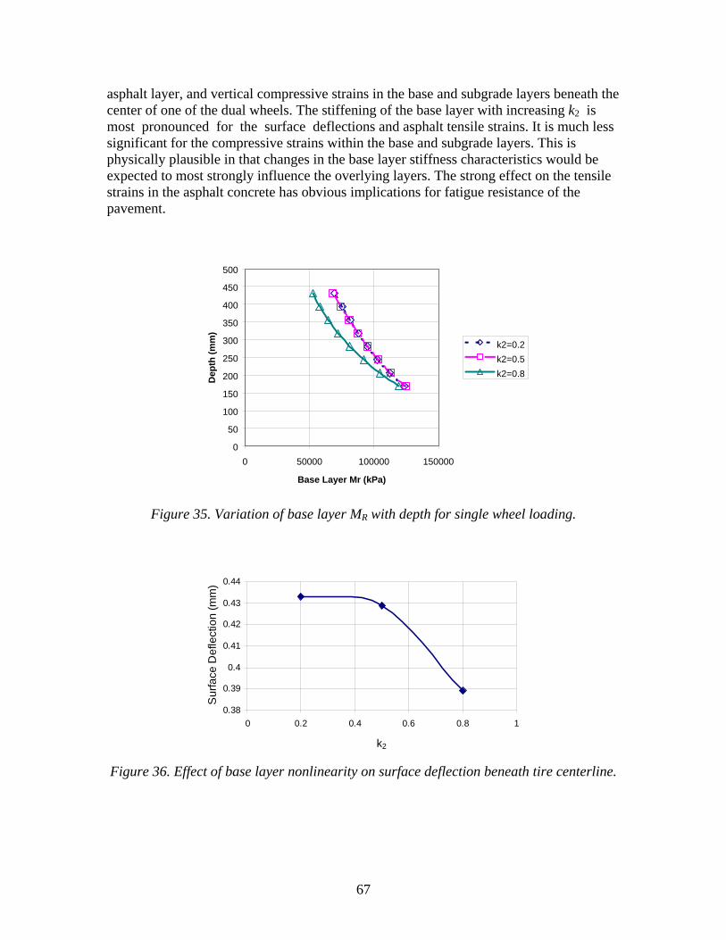
67

asphalt layer, and vertical compressive strains in the base and subgrade layers beneath the center of one of the dual wheels. The stiffening of the base layer with increasing k2 is most pronounced for the surface deflections and asphalt tensile strains. It is much less significant for the compressive strains within the base and subgrade layers. This is physically plausible in that changes in the base layer stiffness characteristics would be expected to most strongly influence the overlying layers. The strong effect on the tensile strains in the asphalt concrete has obvious implications for fatigue resistance of the pavement.

0

50

100

150

200

250

300

350

400

450

500

0 50000 100000 150000

Base Layer Mr (kPa)

Dep

th (m

m)

k2=0.2k2=0.5k2=0.8

Figure 35. Variation of base layer MR with depth for single wheel loading.

0.38

0.39

0.4

0.41

0.42

0.43

0.44

0 0.2 0.4 0.6 0.8 1

k2

Sur

face

Def

lect

ion

(mm

)

Figure 36. Effect of base layer nonlinearity on surface deflection beneath tire centerline.

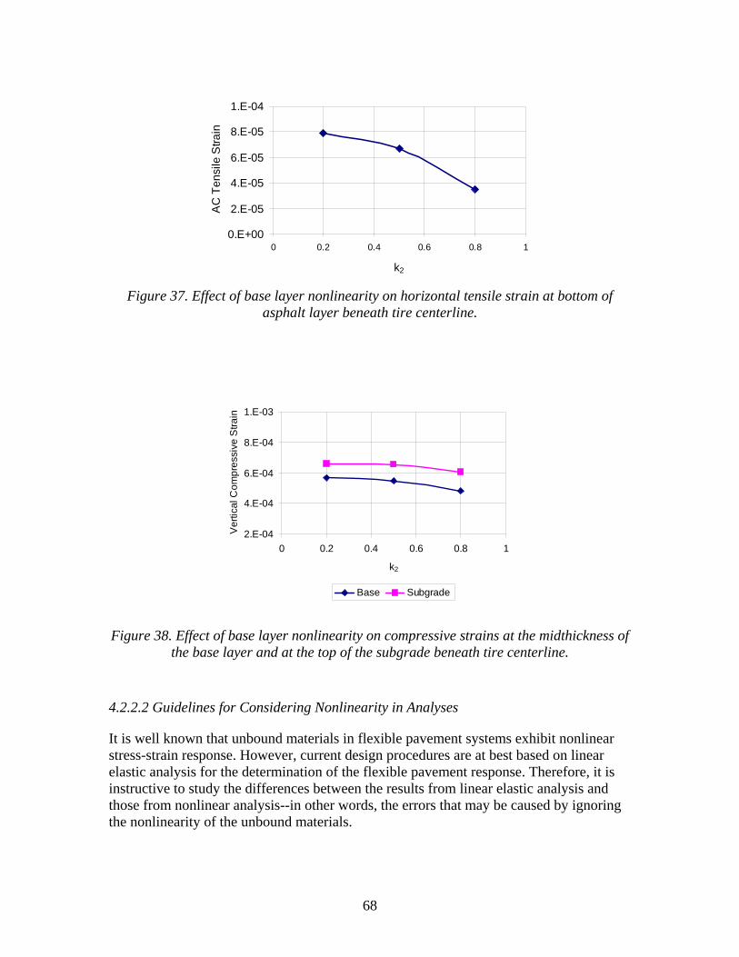
68

0.E+00

2.E-05

4.E-05

6.E-05

8.E-05

1.E-04

0 0.2 0.4 0.6 0.8 1

k2

AC

Ten

sile

Stra

in

Figure 37. Effect of base layer nonlinearity on horizontal tensile strain at bottom of

asphalt layer beneath tire centerline.

2.E-04

4.E-04

6.E-04

8.E-04

1.E-03

0 0.2 0.4 0.6 0.8 1

k2

Ver

tical

Com

pres

sive

Stra

in

Base Subgrade

Figure 38. Effect of base layer nonlinearity on compressive strains at the midthickness of the base layer and at the top of the subgrade beneath tire centerline.

4.2.2.2 Guidelines for Considering Nonlinearity in Analyses

It is well known that unbound materials in flexible pavement systems exhibit nonlinear stress-strain response. However, current design procedures are at best based on linear elastic analysis for the determination of the flexible pavement response. Therefore, it is instructive to study the differences between the results from linear elastic analysis and those from nonlinear analysis--in other words, the errors that may be caused by ignoring the nonlinearity of the unbound materials.

69

The objective of the study described in this section is to determine pavement analysis scenarios in which nonlinearity of the unbound pavement materials is likely to be important. The study is based on comparisons of 2D linear axisymmetric solutions against corresponding nonlinear 2D finite element solutions for a specific set of response parameters. The importance of unbound material nonlinearity will be a function of the inherent nonlinearity of the material (i.e., its ki values) and the induced stress changes, which in turn are a function of the pavement structure. Consequently, both material properties and pavement structure (layer thicknesses and asphalt concrete stiffness) were varied in this study.0 Two typical pavement structure were analyzed. The first is designed for heavy traffic conditions (W18 = 25 million ESALs according to the 1993 AASHTO Pavement Design Guide). As shown in Figure 39a, it consists of 200 mm of asphalt concrete over 450 mm of crushed stone base on natural subgrade. The other is designed for fairly light traffic conditions (W18 = 100 thousand ESALs according to the 1993 AASHTO Pavement Design Guide). As depicted in Figure 39b, it consists of 50 mm of asphalt concrete over 225 mm of crushed stone base on natural subgrade. In both cases, the tire contact pressure is 550 kPa over a circular contact area having a radius of 150 mm. The DSC2D finite element analysis program was used for all analyses reported in this section. The finite element mesh took advantage of the axial symmetry of the problem. Infinite boundary elements were also used at the distant mesh boundaries (see Section 4.3 later). The zone of most interest for the present investigation is the region immediately beneath the tire where the stress and strain gradients are largest and where any material nonlinearity will be most evident. For the heavy traffic pavement structure (Figure 39a), the finite element mesh was truncated with infinite boundaries at a depth of 725 mm beneath the surface and at a horizontal distance of 1050 mm from the centerline of the wheel loading. The final mesh consisted of 483 4-node rectangular elements and 527 nodes. The AC layer was divided into 8 element layers while the base was divided into 12 element layers. For the light traffic pavement structure (Figure 39b), the finite element mesh was truncated with infinite boundaries at a depth of 350 mm beneath the surface and at a horizontal distance of 1050 mm from the centerline of the wheel loading. The final mesh consisted of 1025 4-node rectangular elements and 1117 nodes. The AC thickness was divided into 8 element layers while the base was divided into 12 element layers. The AC and subgrade layers were modeled as conventional isotropic linearly elastic materials. The stiffness of the crushed stone base layer was modeled using the nonlinear resilient modulus defined previously in Eq. (8), with the simplifying conditions of k6=0 and k7=1 as adopted for the 2002 Design Guide. Although the stiffness of natural subgrades is also expected to be stress dependent, it was not considered in this study based on the reasoning that the largest stress changes--and therefore the largest stress-

70

induced stiffness changes--will occur in the unbound material closest to the wheel load, i.e., the base layer. Figure 40 through Figure 42 graphically summarize the influence of stress on resilient modulus for some typical material conditions for both the high traffic and low traffic pavement structures. The upper AC layer and the lower subgrade layer are both treated as linearly elastic materials (EAC=12,500,000 kPa and ESubgrade=50,000 kPa) and all material nonlinearity is concentrated in the granular base layer in all cases. The contours for resilient modulus of the base layer in all of these figures is normalized by the depth-dependent in situ MR values (i.e., the stress dependent MR value under in situ stress conditions alone). Figure 40 shows conditions for a moderately stress stiffening material having k1=2000, k2=0.5, and k3=0. The increase in MR at the top of the base layer beneath the wheel load is evident for both the high traffic (Figure 40a) and low traffic (Figure 40b) designs, but it is much more pronounced in the low traffic structure because of the higher wheel load stresses transmitted through the thin AC layer to the base layer. (Note that the contour intervals are not the same in the two figures.) The moduli values trend toward the in situ values (i.e., contour value equal to 1) with increasing radial distance from the wheel load (i.e., the right edge of the color contour plots). Figure 41 shows conditions for a moderately stress softening material having k1=3000, k2=0, and k3= -0.75. Now MR decreases beneath the wheel load, with the effect more pronounced at the top of the base layer. This stress softening is evident for both the high traffic (Figure 41a) and low traffic (Figure 41b) designs, but it is again much more pronounced in the low traffic structure because of the higher wheel load stresses transmitted through the thin AC layer to the base layer. (Note that the contour intervals are different in the two figures.) The moduli values again trend toward the in situ values with increasing radial distance from the wheel load. Figure 42 shows conditions for a mixed stress stiffening/stress softening material having k1=2500, k2=0.5, and k3= -0.75. As expected, the stress stiffening and stress softening tendencies tend to cancel each other. For the high traffic structure (Figure 42a), the net effect is a very slight stress softening (note the small intervals between the contour values), while for the low traffic structure (i.e., thin AC layer, Figure 42b), a more substantial stress stiffening effect predominates.

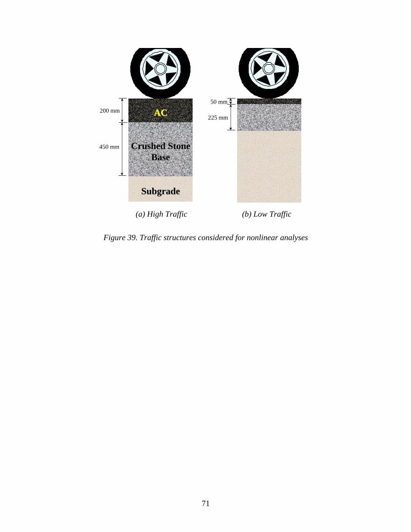
71

50 mm

225 mm

Crushed StoneCrushed StoneBaseBase

SubgradeSubgrade

200 mm

450 mm

ACAC

(a) High Traffic (b) Low Traffic

Figure 39. Traffic structures considered for nonlinear analyses

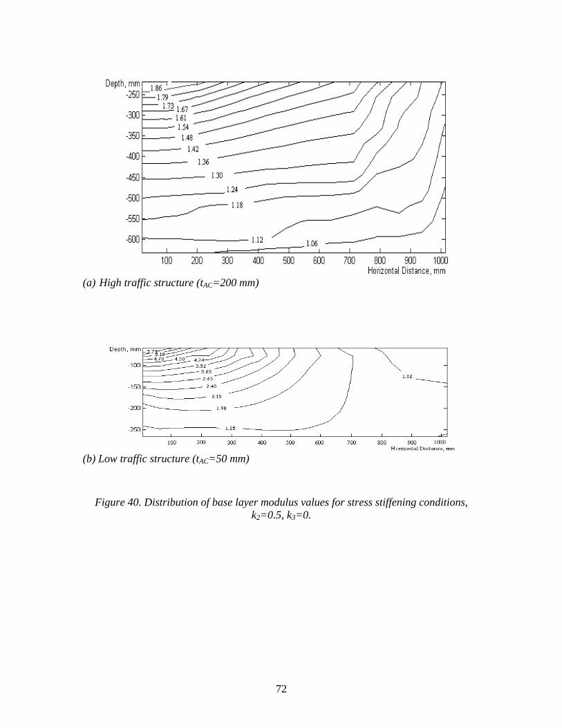
72

(a) High traffic structure (tAC=200 mm)

(b) Low traffic structure (tAC=50 mm)

Figure 40. Distribution of base layer modulus values for stress stiffening conditions, k2=0.5, k3=0.

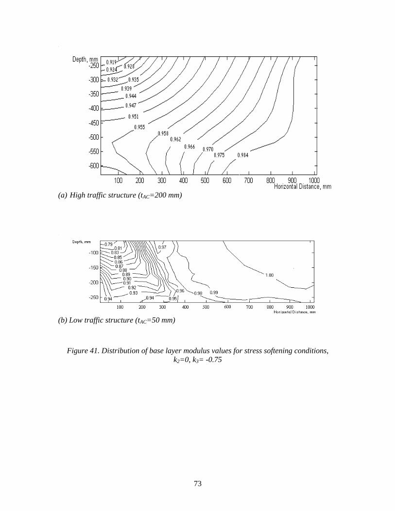
73

(a) High traffic structure (tAC=200 mm)

(b) Low traffic structure (tAC=50 mm)

Figure 41. Distribution of base layer modulus values for stress softening conditions, k2=0, k3= -0.75

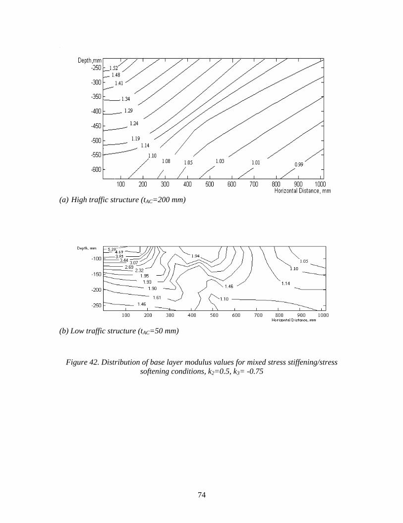
74

(a) High traffic structure (tAC=200 mm)

(b) Low traffic structure (tAC=50 mm)

Figure 42. Distribution of base layer modulus values for mixed stress stiffening/stress softening conditions, k2=0.5, k3= -0.75

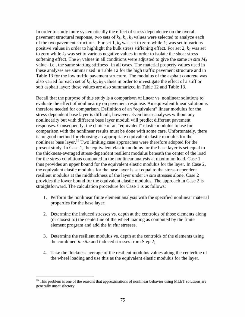
75

In order to study more systematically the effect of stress dependence on the overall pavement structural response, two sets of k1, k2, k3 values were selected to analyze each of the two pavement structures. For set 1, k3 was set to zero while k2 was set to various positive values in order to highlight the bulk stress stiffening effect. For set 2, k2 was set to zero while k3 was set to various negative values in order to isolate the shear stress softening effect. The k1 values in all conditions were adjusted to give the same in situ MR value--i.e., the same starting stiffness--in all cases. The material property values used in these analyses are summarized in Table 12 for the high traffic pavement structure and in Table 13 for the low traffic pavement structure. The modulus of the asphalt concrete was also varied for each set of k1, k2, k3 values in order to investigate the effect of a stiff or soft asphalt layer; these values are also summarized in Table 12 and Table 13. Recall that the purpose of this study is a comparison of linear vs. nonlinear solutions to evaluate the effect of nonlinearity on pavement response. An equivalent linear solution is therefore needed for comparison. Definition of an “equivalent” linear modulus for the stress-dependent base layer is difficult, however. Even linear analyses without any nonlinearity but with different base layer moduli will predict different pavement responses. Consequently, the choice of an “equivalent” elastic modulus to use for comparison with the nonlinear results must be done with some care. Unfortunately, there is no good method for choosing an appropriate equivalent elastic modulus for the nonlinear base layer.16 Two limiting case approaches were therefore adopted for the present study. In Case 1, the equivalent elastic modulus for the base layer is set equal to the thickness-averaged stress-dependent resilient modulus beneath the center of the load for the stress conditions computed in the nonlinear analysis at maximum load. Case 1 thus provides an upper bound for the equivalent elastic modulus for the layer. In Case 2, the equivalent elastic modulus for the base layer is set equal to the stress-dependent resilient modulus at the midthickness of the layer under in situ stresses alone. Case 2 provides the lower bound for the equivalent elastic modulus. The approach in Case 2 is straightforward. The calculation procedure for Case 1 is as follows:

1. Perform the nonlinear finite element analysis with the specified nonlinear material properties for the base layer;

2. Determine the induced stresses vs. depth at the centroids of those elements along (or closest to) the centerline of the wheel loading as computed by the finite element program and add the in situ stresses.

3. Determine the resilient modulus vs. depth at the centroids of the elements using the combined in situ and induced stresses from Step 2;

4. Take the thickness average of the resilient modulus values along the centerline of the wheel loading and use this as the equivalent elastic modulus for the layer.

16 This problem is one of the reasons that approximations of nonlinear behavior using MLET solutions are generally unsatisfactory.

76

Of course, the procedure outlined above for Case 1 cannot be applied unless one has first performed the nonlinear analysis. However, this procedure arguably minimizes any differences between the linear and nonlinear solutions caused by the overall differences in the relative stiffnesses of the layers and thus represents the best-case scenario that minimizes the differences between the nonlinear and equivalent linear analyses. The equivalent linear analysis based on the in situ MR in Case 2 might then be interpreted as a worst-case scenario--i.e., one that maximizes the differences between the nonlinear and equivalent linear analyses. The equivalent elastic moduli of the base layer computed for both cases are summarized in Table 12 and Table 13.

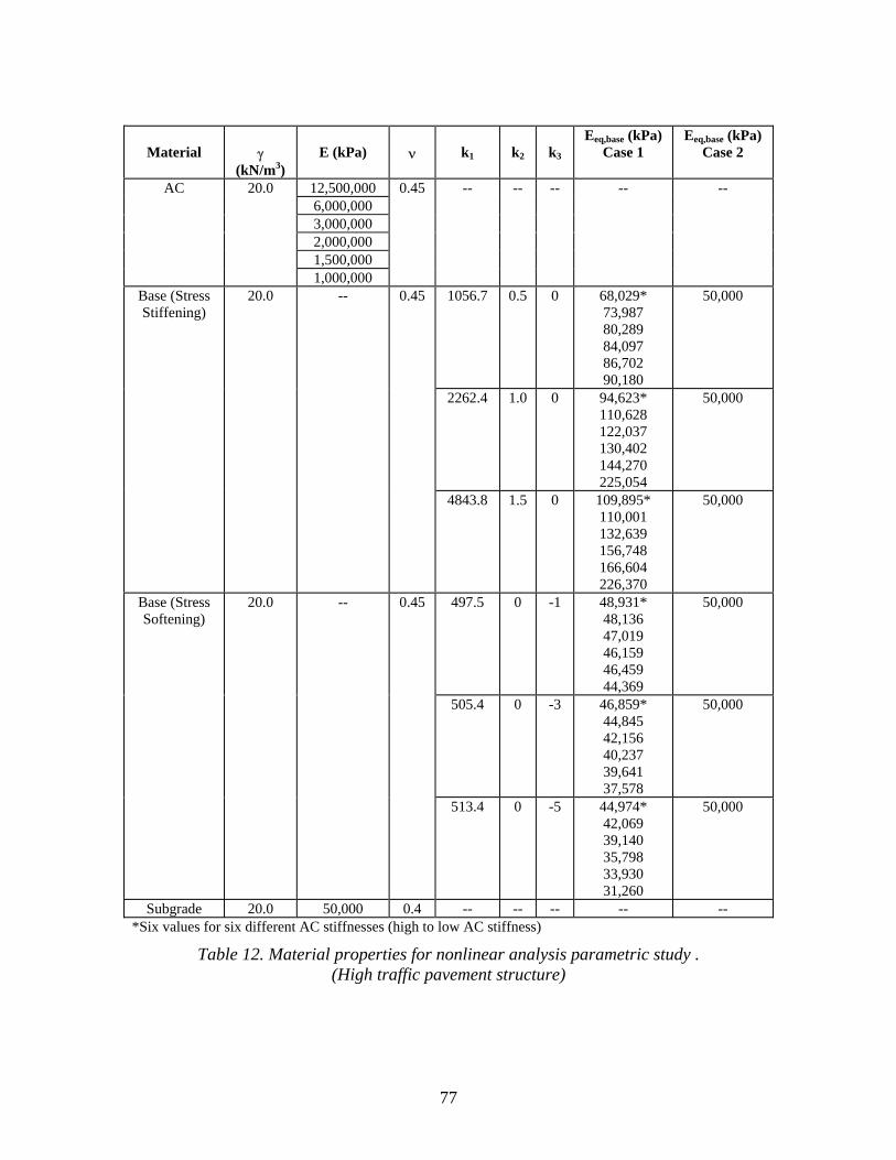
77

Material γ

(kN/m3)

E (kPa)

ν

k1

k2

k3

Eeq,base (kPa) Case 1

Eeq,base (kPa) Case 2

12,500,000 6,000,000 3,000,000 2,000,000 1,500,000

AC 20.0

1,000,000

0.45 -- -- -- -- --

1056.7 0.5 0 68,029* 73,987 80,289 84,097 86,702 90,180

50,000

2262.4 1.0 0 94,623* 110,628 122,037 130,402 144,270 225,054

50,000

Base (Stress Stiffening)

20.0 -- 0.45

4843.8 1.5 0 109,895* 110,001 132,639 156,748 166,604 226,370

50,000

497.5 0 -1 48,931* 48,136 47,019 46,159 46,459 44,369

50,000

505.4 0 -3 46,859* 44,845 42,156 40,237 39,641 37,578

50,000

Base (Stress Softening)

20.0 -- 0.45

513.4 0 -5 44,974* 42,069 39,140 35,798 33,930 31,260

50,000

Subgrade 20.0 50,000 0.4 -- -- -- -- -- *Six values for six different AC stiffnesses (high to low AC stiffness)

Table 12. Material properties for nonlinear analysis parametric study . (High traffic pavement structure)

78

Material γ

(kN/m3)

E (kPa)

ν

k1

k2

k3

Eeq,base (kPa) Case 1

Eeq,base (kPa) Case 2

12,500,000 6,000,000 3,000,000 2,000,000 1,500,000

AC 20.0

1,000,000

0.45 -- -- -- -- --

1709.0 0.5 0 141,420* 161,059 172,815 173,492 176,288 185,840

31,000

591.7 1.0 0 143,165* 186,037 207,018 219,525 222,751 241,688

31,000

Base (Stress Stiffening)

20.0 -- 0.45

495.1 0 -1 48,931*

48,136 47,019 46,159 46,459 44,369

31,000

498.1 0 -3 46,859* 44,845 42,156 40,237 39,641 37,578

31,000

Base (Stress Softening)

20.0 -- 0.45

501.1 0 -5 44,974* 42,069 39,140 35,798 33,930 31,260

31,000

Subgrade 20.0 50,000 0.4 -- -- -- -- -- *Six values for six different AC stiffnesses (high to low AC stiffness)

Table 13. Material properties for nonlinear analysis parametric study. (Low traffic pavement structure)

79

For the purposes of this study, the results obtained from the nonlinear analyses are taken as the “correct” stress and strain distributions and the differences between the linear and nonlinear analysis results are taken as the “errors” in the linear elastic analysis approach. Two critical response parameters were selected for evaluation of the analysis errors: the maximum horizontal tensile strain at the bottom of the asphalt layer, and the maximum vertical compressive strain at the top of the subgrade. Error is defined as follows:

( ) ( )( )

Linear result Nonlinear resultError 100%

Nonlinear result−

= × (33)

As described previously, two different approaches were used to determine the equivalent elastic modulus for the base layer in the linear analyses. Consequently, two types of error values--Type 1 and Type 2--are computed for each nonlinear analysis, corresponding to Case 1 and Case 2 for the equivalent elastic base modulus, respectively. Analyses were performed for both pavement structures for a range of asphalt moduli. The influence of pavement structure (thick vs. thin asphalt layer, corresponding to high and low traffic designs) and asphalt modulus is quantified in terms of a dimensionles sstiffness ratio:

( )

( )3

30

AC

R Base

EtSR

M t= (34)

in which MR0 is the in situ resilient modulus (i.e., the stress-dependent resilient modulus under in situ stress conditions) for the base layer. Figure 43 shows the Type 1 error vs. stiffness ratio as calculated for the high traffic pavement structure and stress stiffening conditions. The linear analysis underpredicts the asphalt tensile strain (Figure 43a) by 30% or more for very flexible asphalt layers (i.e., low values of stiffness ratio) and the largest degree of stress stiffening (i.e., k2=1.5). The Type 1 errors for subgrade compressive strain (Figure 43b) are sometimes positive (overprediction by linear analysis) and sometimes negative (underprediction by linear analysis) and reach values of over 30% for very flexible asphalt conditions (low stiffness ratio values). In both cases, the errors decrease with increasing asphalt stiffness (increasing stiffness ratio); for stiffness ratio values greater than 4 or 5, the Type 1 errors in Figure 43 are all less than 5%. Figure 44 shows the corresponding Type 2 errors for these conditions. Now the linear analysis consistently overpredicts the asphalt tensile strains; this is sensible given the substantially lower equivalent elastic modulus for the base layer for the Case 2 assumptions. The under/overprediction of subgrade strains is again variable, but as was the case for the Type 1 errors (Figure 43), the error values all decrease as stiffness ratio increases. Corresponding results are shown in Figure 45 (Type 1 errors) and Figure 46 (Type 2 errors) for the high traffic structure and strain softening base behavior, in Figure 47 (Type

80

1 errors) and Figure 48 (Type 2 errors) for the low traffic structure and strain stiffening behavior, and in Figure 49 (Type 1 errors) and Figure 50 (Type 2 errors) for the low traffic structure and strain softening behavior. Overall observations drawn from Figure 43 through Figure 50 are as follows: • The Type 2 errors are consistently higher than the Type 1 errors. This implies that

determining the equivalent elastic modulus for the base layer from the in situ stress conditions is not satisfactory (as might be expected intuitively). As previously mentioned, though, the difficulty with the Type 1 error is that a nonlinear analysis must first be performed to determine the equivalent elastic modulus for the base layer (Case 1 for base layer modulus); this defeats the whole point of performing an equivalent linear analysis.

• The maximum errors in some of the cases are on the order of hundreds of percent; this magnitude of error can be expected to have a serious detrimental effect on pavement performance prediction accuracy. This is a strong argument for incorporation of unbound material nonlinearity in these analyses.

• At corresponding values of stiffness ratio, the low traffic structure consistently gives

larger error values than does the high traffic structure. It appears that the stiffness ratio does not capture perfectly the influence of relative stiffness of the layers.

• In all cases the errors decrease as the stiffness ratio increases--i.e., as the stiffness of the asphalt layer increases relative to the stiffness of the base layer. With only few exceptions, the error levels fall below 5 to 10% at stiffness ratios greater than 4 to 6. This applies regardless of the error type (Type 1 or Type 2), pavement structure (high traffic or low traffic design), or response quantity (asphalt tensile strain or subgrade compressive strain). This implies that nonlinear base material behavior should be considered whenever the stiffness ratio in Eq. (34) is less than 4 to 6.

Of course, the parametric conditions investigated in this study are necessarily limited. Nonetheless, it is clear that nonlinear unbound material behavior becomes increasingly important for low stiffness ratios--i.e., for low asphalt moduli (i.e., hot climate/high pavement temperature) and/or thin asphalt layers. These results thus provide some guidance regarding conditions under which incorporation of nonlinear material behavior in design calculations is important, at least for unbound base layers. Although subgrade nonlinearity has not been considered in this study, the trends observed for the base layer should extend to the subgrade as well. Low overlying pavement stiffness (whether due to modulus or thickness of the asphalt, base, or subbase layers) will elevate the induced stresses within the subgrade and therefore activate any stress dependent behavior of the material. As a preliminary rule of thumb, one could compute the stiffness ratio in Eq. (34) using an equivalent Et3 for all of the overlying layers. The guidelines from the nonlinear base layer analyses suggest that nonlinear subgrade behavior should be included in the flexible pavement response analyses when the stiffness ratio using this equivalent Et3is less than 4 to 6.

81

-30

-25

-20

-15

-10

-5

00 3 6 9 12 15

(Et^3)AC/(MR0t^3)base

k1=1056.7, k2=0.5, k3=0k1=2262.4, k2=1.0, k3=0k1=4843.8, k2=1.5, k3=0

(a) AC tensile strains.

-40

-30

-20

-10

0

10

20

30

40

0 3 6 9 12 15(Et^3)AC/(MR0t^3)base

k1=1056.7, k2=0.5, k3=0k1=2262.4, k2=1.0, k3=0k1=4843.8, k2=1.5, k3=0

(b) Subgrade compressive strains.

Figure 43. Type 1 errors: High traffic structure, stress stiffening conditions (k2>0, k3=0). (a) AC tensile strains. (b) Subgrade compressive strains.

82

0

10

20

30

40

50

60

0 3 6 9 12 15(Et^3)AC/(MR0t^0)base

k1=1056.7, k2=0.5, k3=0k1=2262.4, k2=1.0, k3=0k1=4843.8, k2=1.5, k3=0

(a) AC tensile strains.

-80

-60

-40

-20

0

20

40

0 3 6 9 12 15

(Et^3)AC/(MR0t^3)base

k1=1056.7, k2=0.5, k3=0k1=2262.4, k2=1.0, k3=0k1=4843.8, k2=1.5, k3=0

(b) Subgrade compressive strains.

Figure 44. Type 2 errors: High traffic structure, stress stiffening conditions (k2>0, k3=0). (a) AC tensile strains. (b) Subgrade compressive strains.

83

0

1

2

3

4

5

0 3 6 9 12 15(Et^3)AC/(MR0t^3)base

k1=497.5, k2=0, k3=-1k1=505.4, k2=0, k3=-3k1=513.4, k2=0, k3=-5

(a) AC tensile strains.

0

1

2

3

4

5

0 3 6 9 12 15(Et^3)AC/(MR0t^3)base

k1=497.5, k2=0, k3=-1k1=505.4, k2=0, k3=-3k1=513.4, k2=0, k3=-5

(b) Subgrade compressive strains.

Figure 45. Type 1 errors: High traffic structure, stress softening conditions (k2=0, k3<0). (a) AC tensile strains. (b) Subgrade compressive strains.

84

-10

-8

-6

-4

-2

00 3 6 9 12 15

(Et^3)AC/(MR0t^3)base

k1=497.5, k2=0, k3=-1k1=505.4, k2=0, k3=-3k1=513.4, k2=0, k3=-5

(a) AC tensile strains.

-10

-8

-6

-4

-2

00 3 6 9 12 15

(Et^3)AC/(MR0t^3)base

k1=497.5, k2=0, k3=-1k1=505.4, k2=0, k3=-5k1=513.4, k2=0, k3=-5

(b) Subgrade compressive strains.

Figure 46. Type 2 errors: High traffic structure, stress softening conditions (k2=0, k3<0). (a) AC tensile strains. (b) Subgrade compressive strains.

85

-140

-120

-100

-80

-60

-40

-20

00 0.5 1 1.5 2 2.5 3

(Et^3)AC(MR0^3)base

k1=1709,k2=0.5,k3=0k1=5917,k2=1.0,k3=0

(a) AC tensile strains.

-120

-100

-80

-60

-40

-20

00 0.5 1 1.5 2 2.5 3

(Et^3)AC/(MR0^3)base

k1=1709,k2=0.5,k3=0k1=5917,k2=1.0,k3=0

(b) Subgrade compressive strains.

Figure 47. Type 1 errors: Low traffic structure, stress stiffening conditions (k2>0, k3=0). (a) AC tensile strains. (b) Subgrade compressive strains.

86

0

200

400

600

800

1000

0 0.5 1 1.5 2 2.5 3

(Et^3)AC/(MR0^3)base

k1=1709,k2=0.5,k3=0k1=5917,k2=1.0,k3=0

(a) AC tensile strains.

0

50

100

150

200

250

300

0 0.5 1 1.5 2 2.5 3

(Et^3)AC/(MR0 3̂)base

k1=1709,k2=0.5,k3=0k1=5917,k2=1.0,k3=0

(a) Compressive subgrade strains.

Figure 48. Type 2 errors: Low traffic structure, stress stiffening conditions (k2>0, k3=0). (a) AC tensile strains. (b) Subgrade compressive strains.

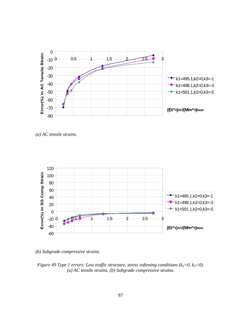
87

-80

-70

-60

-50

-40

-30

-20

-10

00 0.5 1 1.5 2 2.5 3

(Et^3)AC/(MR0^3)base

k1=495.1,k2=0,k3=-1k1=498.1,k2=0,k3=-3k1=501.1,k2=0,k3=-5

(a) AC tensile strains.

-60

-40

-20

0

20

40

60

80

100

120

0 0.5 1 1.5 2 2.5 3

(Et^3)AC/(MR0^3)base

k1=495.1,k2=0,k3=-1k1=498.1,k2=0,k3=-3k1=501.1,k2=0,k3=-5

(b) Subgrade compressive strains.

Figure 49 Type 1 errors: Low traffic structure, stress softening conditions (k2=0, k3<0). (a) AC tensile strains. (b) Subgrade compressive strains.

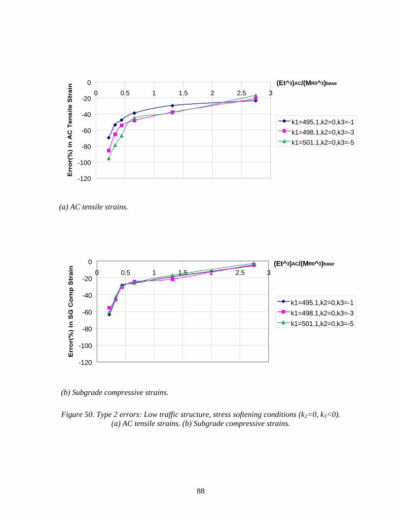
88

-120

-100

-80

-60

-40

-20

00 0.5 1 1.5 2 2.5 3

(Et^3)AC/(MR0^3)base

k1=495.1,k2=0,k3=-1k1=498.1,k2=0,k3=-3k1=501.1,k2=0,k3=-5

(a) AC tensile strains.

-120

-100

-80

-60

-40

-20

00 0.5 1 1.5 2 2.5 3

(Et^3)AC/(MR0^3)base

k1=495.1,k2=0,k3=-1k1=498.1,k2=0,k3=-3k1=501.1,k2=0,k3=-5

(b) Subgrade compressive strains.

Figure 50. Type 2 errors: Low traffic structure, stress softening conditions (k2=0, k3<0). (a) AC tensile strains. (b) Subgrade compressive strains.

89

4.2.3 Nonlinear Superposition

4.2.3.1 The Problem

Flexible pavement structural analysis for design purposes must consider (as a minimum) multiple wheel/axle loading configurations, seasonal variations of material layer properties, and the nonlinear behavior of unbound materials. There is no dispute that these requirements can all be easily satisfied by nonlinear three-dimensional finite element techniques. The capabilities of three-dimensional finite elements for flexible pavement structural analysis are already well-established in the literature (Chen et al., 1995; Cho, McCullough, and Weissmann, 1996; Hjelmstad, Kim, and Zuo, 1997; Shoukry (1998a), Uddin, 1998; White, 1998; Zaghoul and White, 1993) and have been the focus of at least two recent conferences (Hermann, 1997; Shoukry, 1998b) and a report from the U.S. General Accounting Office (GAO, 1997). However, the computation times required for three-dimensional finite element analysis—even with the computer capabilities available to highway agencies today—are too long for routine practical design usage. As is often the case in engineering design, compromises must be made between analytical precision and model realism. One such compromise is to retain seasonal property variations and material nonlinearity within a two-dimensional axisymmetric single wheel finite element model and to approximate multiple wheel effects via superposition. Although superposition of nonlinear solutions is undeniably invalid from a rigorous theoretical viewpoint, the inevitable errors from this approach may be well within acceptable magnitudes for practical design purposes. For example, early field studies conducted by the U.S. Army Corps of Engineers found that stresses and deflections measured under plate load tests and multiple aircraft gear loadings could be reasonably predicted using superposition principles despite the nonlinearity of the unbound layers (USACE, 1951; USACE, 1954; Ahlvin et al., 1971; Chou and Ledbetter (1973); all as reported in Thompson and Garg, 1999). Uzan (Texas Transportation Institute, 1991) approached this isssue during the Strategic Highway Research Program (SHRP) via axisymmetric nonlinear solutions for concentric axisymmetric circle and ring loads. He found that the maximum errors in the computed stresses and displacements from the nonlinear superposition computations were on the order of 20%. Uzan put these errors in context by illustrating that they are only slightly larger than the errors resulting from modeling nonuniform real tire pressure distributions with an equivalent uniform contact pressure—an error level that is comfortably, albeit implicitly, accepted in current practice. Based on these findings, the nonlinear superposition approach was adopted for the original SHRP flexible pavement performance prediction system (Lytton et al., 1993). Of course, axisymmetric analyses of the type conducted by Uzan cannot address nonlinear superposition of side-by-side multiple wheel and axle loads. This requires a fully 3D nonlinear analysis of the type described in the present paper. Specifically, the case considered here is a dual wheel loading on a pavement structure having a stress

90

dependent base layer. This system is analyzed as a fully 3D problem, and the rigorous stresses and strains are then compared against predictions from superimposed single wheel load nonlinear solutions for the same pavement structure. The focus is on errors in the critical pavement response quantities of interest in mechanistic-empirical design methods: tensile stresses/strains at the bottom of the AC layer; compressive stresses/strains at the top of the subgrade; and maximum surface deflection. The objective of this study is limited to comparisons of an approximate solution (superimposed 2D axisymmetric nonlinear finite element) against a more rigorous approach (3D nonlinear finite element) for a very specific set of response parameters. The issue of how closely either of these solutions matches actual field data is not addressed, although others have documented that careful pavement structural analysis can reproduce field-measured stresses and strains with some fidelity (Ullidtz, 1998; see also Section 1.2). The more sophisticated three-dimensional finite element solutions are simply used in this study as a standard for evaluating the consequences of modeling approximations and simplifications. This is an entirely appropriate use for 3D finite element analysis. As a final perspective, there clearly are many potential sources of error in pavement design analyses. The traffic loading, environmental conditions, and material property inputs, the pavement structural analysis algorithm, and the pavement performance models all have varying degrees of associated inaccuracy and/or uncertainty. In most designs, the level of inaccuracy and/or uncertainty in the material inputs and the pavement performance models is considerably greater than that from the pavement structural analysis model. As succinctly put by Thompson and colleagues (Thompson, 1990):

“The development of more sophisticated/complex/realistic structural models does not necessarily insure an ‘improved’ pavement design procedure. In fact, the structural model is frequently the ‘most advanced’ component! INPUTS and TRANSFER FUNCTIONS [pavement performance models] are generally the components lacking precision.”

In other words, the errors from nonlinear superposition must be evaluated within the context of all other errors in the pavement design methodology.

4.2.3.2 Analysis Description

A series of finite element analyses were performed to quantify the errors resulting from the superposition of nonlinear 2D solutions. Instead of a comprehensive parameteric study, the investigation focused on a pavement scenario intended to maximize the errors from the nonlinear superposition. Only stress dependence of the crushed stone base layer was considered in the study. A relatively flexible AC layer and a moderately stiff subgrade were selected to maximize the stresses in the base layer and thus the influence of the base layer stress dependence upon the computed response. These selections were designed to provide upper bound estimates for the errors resulting from the nonlinear superposition.

91

The pavement structure analyzed in this study consisted of 150 mm of asphalt concrete over 300 mm of crushed stone base on natural subgrade. The idealized vehicle load consisted of a single dual wheel axle with a total load on each wheel of 20 kN. The tire contact pressure was taken as 500 kPa over a square17 contact area of 200 mm x 200 mm. Centerline spacing between the dual wheels was 300 mm. ABAQUS was used for all finite element analyses in this study (Hibbitt, Karlsson, and Sorensen, 1998).18 Because of symmetry19, only one quarter of the problem geometry was discretized with finite elements. For finite element modeling purposes, the problem geometry was truncated with rigid boundaries at a depth of 900 mm beneath the surface and at a horizontal distance of 1500 mm from the center of the dual wheels. The final finite element mesh based on these idealizations (Figure 51 and Figure 52) consisted of 7524 4-node quadrilateral elements, 8740 nodes, and 26,220 degrees of freedom. The AC layer is divided into 4 element layers while the base is divided into 8 layers. Previous analyses using 4-node quad elements have found this level of discretization sufficient for capturing the bending response of the layers (e.g., see Section 1.3.3.1). The AC and subgrade layers were modeled as conventional isotropic linearly elastic materials. The stiffness of the crushed stone base layer was based upon the general stress dependent resilient modulus model given in Eq. (8) as modified for the 2002 Design Guide with k6=0 and k7=1. In addition, only the bulk stress stiffening term in Eq. (8) is considered for the purposes of this study. This is appropriate for the crushed stone material assumed for the stress dependent base layer. The results presented previously in Section 4.2.2.2 also suggest that stress stiffening nonlinear behavior is generally more important than stress softening effects. Equation (8) then simplifies to:

2

1

k

R aa

M k pp

⎛ ⎞= ⎜ ⎟

⎝ ⎠

θ (35)

Eq. (35) is similar to the more familiar two-parameter K-θ model

21

KRM K= θ (36)

differing only by the pa stress normalization term. Table 14 summarizes typical values for the K1 and K2 parameters in Eq. (36) as reported by Huang (1993). These values were converted to typical values for the k1 and k2 parameters in Eq. (35). Representative values from Table 14 of K1 ≈ 5000 psi and K2=0.5 in Eq. (36) at a value of θ ≈ 1 atmosphere (MR=18,500 psi or 128,000 kPa) correspond to values of k1 ≈ 1300 (dimensionless) and

17 Since these analyses were not concerned with the detailed stress and strain fields in the immediate vicinity of the tire contact plane, the differences between square and circular tire footprints were judged to be unimportant. 18 This study was conducted early during the NCHRP 1-37A project before the DSC2D finite element program had been selected and modified. 19 Only the dual wheels on one end of the axle were analyzed. The other end of the axle was assumed to be far enough away that interaction effects were neglible.

92

k2=0.5 in Eq. (35). In order to study the effect of degree of stress dependence for MR, additional values of 0.2 and 0.8 were selected for k2, and corresponding k1 values were determined such that the MR value at θ ≈ 1 atmosphere remained constant. The influence of the degree of stress dependence of the stress-strain curves is illustrated in Figure 53. The initial confining pressure 6.9 kPa (1 psi) for the curves in Figure 53 is approximately equal to the in situ confining stress at the center of the base layer. Incorporation of the material model defined by Eq. (35) into ABAQUS was performed using the *HYPOELASTIC material model. Eq. (35) was used to develop secant MR and first strain invariant I1=ε1+ε2+ε3 values over a range of θ. The secant MR values were numerically converted to tangent modulus E values for input as a function of I1 in the standard ABAQUS *HYPOELASTIC material model. A tension cut-off was imposed by specifying a very small E for tensile I1 values. The final k1 and k2 values and the other material property values used in the analyses are summarized in Table 15. The ABAQUS finite element model was verified in a linearly elastic mode via comparisons with independent results from multilayer elastic theory (MLET) using the KENLAYER program (Huang, 1993). Two cases were considered for the KENLAYER MLET analyses: (a) the subgrade extending to infinite depth; and (b) a rigid layer underlying the subgrade at a depth corresponding to the bottom of the finite element mesh. Negligible differences were found in the computed stresses and strains between these two cases, despite the fact that the finite element boundaries are closer than conventional meshing guidelines would suggest. The computed vertical and radial stresses from the ABAQUS linear finite element computations agreed very closely with the KENLAYER MLET results at all centerline depths, as expected

4.2.3.3 Analysis Results

Nonlinear 3D finite element analyses were performed for single wheel and dual wheel loadings for each of the three k1, k2 combinations given in Table 15. The same finite element mesh, boundary conditions, material properties (other than k1, k2), and tire loads/pressures were used for all analyses; the only parameter that varied was the load geometry (single vs. dual). Note that even though the single wheel analysis could have been performed rigorously in an axisymmetric mode (replacing the square tire contact area with a circular area), this was not done in order to maintain as much consistency as possible between the dual and single wheel solutions. Figure 54 illustrates variation of the stress dependent MR values with depth in the base layer as computed from the single wheel. All results are computed at the centroid of the finite elements in the vertical column nearest the center of the loading (see Figure 52). The results in Figure 54 confirm the physical expectation that the k2=0.8 analysis exhibit the most variation in MR through the thickness while the k2=0.2 analysis exhibit the least. The differences in MR variation between the k2=0.2 and k2=0.5 analyses were much less than would have been expected based on the stress-strain behavior shown in Figure 53, but this is likely due to the differences between the more complex multidimensional stress states in the pavement base layer as compared to the simple uniaxial stress-strain conditions in Figure 53. Thickness-averaged MR values for the base layer in this near-

93

centerline location equaled 93.4, 93.5, and 80.6 MPa for k2=0.2, 0.5, and 0.8, respectively. Note that since the selections of k1 and k2 values in Table 15 are somewhat arbitrary, the thickness-averaged MR values do not necessarily increase as a function of k2. The single wheel nonlinear analysis results were superimposed during post-processing to create the approximate dual wheel nonlinear solution. In addition, linearly elastic single wheel finite element analyses were performed, again using the same mesh but replacing the stress dependent base layer moduli with constant moduli equal to the average through-thickness moduli values calculated from the results in Figure 54. These single wheel linear solutions were also superimposed to create the corresponding dual wheel linear cases. Of course, the selection of equivalent moduli values to use in the linearly elastic analyses is highly arbitrary, and there is no guarantee that an equivalent modulus value that gives the best agreement between linear and nonlinear solutions for one pavement response variable (e.g., tensile strains at the bottom of the asphalt) will also give the best agreement for any of the other pavement response variables (e.g., compressive stress at the top of the subgrade). Nevertheless, setting the equivalent moduli equal to the average moduli in the zone beneath the wheel load for each case is intuitively reasonable. Representative comparisons between the dual wheel nonlinear solutions (labeled Dual NL in the figures), superimposed single wheel nonlinear solutions (labeled S+S NL), and superimposed single wheel linear solutions (S+S L) are shown in Figure 55 through Figure 60 for the case of k2=0.8 (i.e., the highest level of stress dependency considered in these analyses). The qualitative differences between the dual wheel nonlinear solutions (Dual NL) and the superimposed single wheel nonlinear solutions (S+S NL) were smallest for the vertical and horizontal stresses (Figure 55 and Figure 56) and largest for the vertical and horizontal strains (Figure 57 and Figure 58). The qualitative differences for centerline and surface deflections (Figure 59 and Figure 60) were between those for stresses and strains. In all cases, however, the qualitative differences between the dual wheel nonlinear (Dual NL) and superimposed single wheel nonlinear solutions (S+S NL) were smaller than between the Dual NL and superimposed single wheel linear (S+S L) results. Recall that the motivation for this study was to assess the errors in computed values for the critical pavement response variables that are the inputs to empirical performance models in mechanistic-empirical design methods. The critical response variables considered here are: the maximum tensile stress/strain at the bottom of the AC layer; the maximum compressive stress/strain at the top of the subgrade layer; and the maximum surface deflection. Figure 61 through Figure 65 summarize the percentage errors associated with the nonlinear superposition for each of these critical response variables for each of the stress dependence levels as quantified by k2. In each figure, the dual wheel nonlinear solutions (Dual NL) are considered to be the “true” results, and errors are computed as the difference between the superimposed single wheel nonlinear solutions (S+S NL) and these true results; these errors are labeled “Nonlinear” in Figure 61 through Figure 65. The differences between the superimposed single wheel linear solutions (S+S

94

L) and the “true” dual wheel nonlinear solutions (Dual NL) are also shown in Figure 61 through Figure 65 and are labeled “Linear”. As before, all stresses and strains are computed at the centroid of the element closest to the actual critical location for the response variable (see Figure 52 for locations). The largest discrepancies between the Dual NL and S+S NL solutions occur for the tensile stresses and strains in the AC layer, where the S+S NL solution overpredicts the stresses and strains by 25% and 20%, respectively, when k2=0.8 and by 14% and 14%, respectively, when k3=0.5. The errors between the Dual NL and S+S NL solutions for all other critical pavement response variables are less than 10%. Error magnitudes on the order of 25% appear excessive at first glance, but some mitigating factors should be kept in mind. First, the discrepancies between the Dual NL and the superimposed linear single wheel solutions S+S L are substantially larger than those between the nonlinear Dual NL and S+S NL cases. As shown in Figure 61 and Figure 63, the errors in computed tensile stresses and strains in the AC layer for k2=0.8 for the superimposed linear solution S+S L are 133% and 78%, respectively, as compared to the 25% and 20% errors for the S+S NL case. In other words, the errors in tensile stresses and strains due to neglect of nonlinearity effects are 3 to 5 times larger than the errors due to nonlinear superposition. This observation holds for all of the critical pavement response variables in Figure 61 through Figure 65; the S+S L errors are consistently 2 to 5 times larger than the S+S NL errors. Second, recall that the pavement structure was designed to produce an upper bound estimate of the solution error. For most pavement structures, the actual errors would be expected to be considerably less than this upper bound. As an example, Figure 66 shows the changes in error magnitude that occur when the modulus of the AC layer is changed from a low value of 1400 MPa—a value that produces large stresses, and correspondingly large errors, in the base layer—to a high value of 14,000 MPA. The maximum errors of 20% to 25% now drop to errors of 5% to 6%, well within acceptable accuracy for pavement design analyses.

4.2.3.4 Conclusions

Practical engineering design requires tradeoffs, not just in the design itself but also in the methods used to arrive at the design. Superposition of nonlinear 2D axisymmetric solutions undeniably violates rigorous principles of mechanics, but computational constraints make fully 3D nonlinear analyses impractical for routine design usage today. This paper has attempted to estimate upper bounds for the errors attributable to nonlinear superposition for multiple wheel loads. The focus is on errors in the critical pavement response quantities—e.g., AC tensile stresses/strains, subgrade compressive stresses/strains, surface deflections--that are the inputs to the empirical performance models incorporated in mechanistic-empirical design procedures. There are several obvious limitations in the study that must be kept in mind when evaluating the results. First, although designed to produce conditions approaching a “worst case” scenario, only a limited set of pavement structures were considered: one set

95

of layer thicknesses, two asphalt concrete modulus values, three levels of stress dependence for the base layer, and one subgrade stiffness. The nonlinear response of the system was limited to a stress-stiffening crushed stone base layer. Only one wheel configuration was analyzed: a single axle dual wheel system at a fixed 18 kip axle load with uniform tire pressure distribution. Evaluation of errors was based on critical pavement response quantities at the bottom of the asphalt layer and the top of the subgrade, and it is assumed that the results from the rigorous 3D nonlinear finite element analyses represent “truth” for the comparisons. With the above caveats firmly in mind, the overall findings from this study can be summarized as follows: • The largest errors are in the computation of the maximum tensile stresses and strains

at the bottom of the AC layer. These errors ranged up to 25% and 20%, respectively, for the most extreme case of base material stress dependency (k2=0.8) considered in this study.

• The errors in computation of stresses and strains at the top of the subgrade and of the maximum surface deflection were all less than 5% for all of the nonlinear cases considered in this study.

• The discrepancies between the dual wheel nonlinear solution and the superimposed single wheel nonlinear solutions are much smaller—by a factor of 3 to 5—than the discrepancies between the dual wheel nonlinear solution and the superimposed single wheel linear solutions. In other words, the errors caused by neglect of nonlinearity effects are significantly larger than the errors due to nonlinear superposition.

• The nonlinear superposition errors for the critical pavement response quantities depend upon the details of the pavement structure. For example, the errors decrease as the stiffness of the AC layer increases—i.e., for high-traffic designs.

Clearly, there are other sources of nonlinearity—and other sources of analysis error--in pavement systems. Subgrade nonlinearity has not been considered here, nor have multiple axle load configurations. The contributions of these other factors, however, would intuitively be expected to be smaller than the contributions of base layer nonlinearity, particularly for pavement response variables like maximum AC tensile strains. The maximum nonlinear superposition errors encountered in this study—up to 25% for the maximum AC tensile strain—are felt to be realistic upper bounds for realistic pavement structures. These error magnitudes are comparable to those found by Uzan (TTI, 1991) in his purely 2D study and, as pointed out by Uzan, comparable in magnitude to the errors from standard simplifications like substitution of uniform contact stresses for actual tire pressure distributions. These errors would thus seem acceptable for practical design calculations. Lastly, the results from this study should not be construed as an argument against the need for more sophisticated techniques such as nonlinear 3D finite element analysis in

96

pavement analysis and design. These techniques are already used today by highway agencies and others for research studies, forensic investigations, and major special projects. These techniques are also the only rational mechanistic way to analyze reflection and other cracking problems in flexible pavements. These advanced analysis techniques will clearly become more practical for routine design over the next decade as computational power continues to increase. Today’s research and specialized applications of advanced analysis techniques are vital for paving the way for their more routine use in the future.

97

Table 14. Typical values for K1 and K2 (Huang, 1993)

Material K1

(psi) K2

Silty Sand 1620 0.62 Sand-Gravel 4480 0.53

Sand-Aggregate 4350 0.59 Crushed Stone 7210 0.45

Table 15. Material properties for nonlinear superposition analyses

Material E

(MPa) k1 k2 ν γ (kN/m3)

Asphalt Concrete 1,400 0.35 24.0 Base Low stress dependence Medium stress dependence High stress dependence

1278 1305 1333

0.2 0.5 0.8

0.35 0.35 0.35

20.0 20.0 20.0

Subgrade 70 0.35 17.5 Note: k1 and k2 are based on definition in Eq. (35). Combinations of k1 and k2 are based on

a MR value of approximately 128 MPa at θ ≈ 1 atmosphere.

98

7524 elements (4 node quads)8740 nodes26,220 DOF

Figure 51. 3D finite element mesh for nonlinear superposition study

AC

BASE

SUBGRADE

P

Stress/Strain Line

Critical Subgrade Element

Critical AC Element

Figure 52. Cross section of finite element mesh showing calculation locations.

99

0

100

200

300

400

500

600

700

800

0 0.001 0.002 0.003 0.004

Axial Strain

Dev

iato

r Str

ess

(kPa

)

k2=0.2k2=0.5k2=0.8

Figure 53. Degree of stress dependence considered in analyses

(initial confining pressure = 6.9 kPa).

100

0

50

100

150

200

250

300

350

400

450

500

0 50000 100000 150000

Base Layer Mr (kPa)

Dep

th (m

m)

k2=0.2k2=0.5k2=0.8

Figure 54. Variation of base layer MR with depth for single wheel nonlinear solutions.

101

0

100

200

300

400

500

600

0 100 200 300 400 500 600

Vertical Stress (kPa)

Dep

th (m

m)

Dual NL S+S NL S+S L

Figure 55. Variation of vertical stress with depth beneath a wheel for k2=0.8. (Notation: Dual NL = Dual Wheel Nonlinear solution; S+S NL = Superimposed Single Wheel

Nonlinear solution; S+S L = Superimposed Single Wheel Linear solution. See Figure 52 for stress/strain computation locations.)

0

100

200

300

400

500

600

-600 -400 -200 0 200 400 600 800

Horizontal Stress (kPa)

Dep

th (m

m)

Dual NL S+S NL S+S L

Figure 56. Variation of horizontal stress with depth beneath a wheel for k2=0.8. (See Figure 55 caption for notation)

102

0

100

200

300

400

500

600

0 0.0002 0.0004 0.0006 0.0008 0.001 0.0012

Vertical Strain

Dep

th (m

m)

Dual NL S+S NL S+S L

Figure 57. Variation of vertical strain with depth beneath a wheel for k2=0.8. (See Figure 55 caption for notation)

0

100

200

300

400

500

600

-0.0004 -0.0003 -0.0002 -0.0001 0 0.0001 0.0002 0.0003

Horizontal Strain

Dep

th (m

m)

Dual NL S+S NL S+S L

Figure 58. Variation of horizontal strain with depth beneath a wheel for k2=0.8. (See Figure 55 caption for notation)

103

0

100

200

300

400

500

600

700

0 0.1 0.2 0.3 0.4 0.5 0.6

Centerline Vertical Displacement (mm)

Dep

th (m

m)

Dual NL S+S NL S+S L

Figure 59. Variation of vertical displacement with depth beneath a wheel for k2=0.8. (See Figure 55 caption for notation)

0

0.1

0.2

0.3

0.4

0.5

0.6

0 200 400 600 800 1000

Horizontal Distance (mm)

Surf

ace

Def

lect

ion

(mm

)

Dual NL S+S NL S+S L

Figure 60. Surface deflection beneath a wheel for k2=0.8. (See Figure 55 caption for notation)

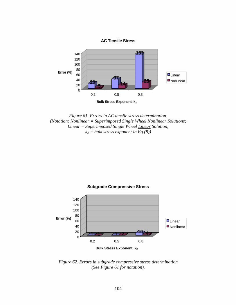
104

205

3714

133

25

020406080

100120140

Error (%)

0.2 0.5 0.8

Bulk Stress Exponent, k2

AC Tensile Stress

LinearNonlinear

Figure 61. Errors in AC tensile stress determination.

(Notation: Nonlinear = Superimposed Single Wheel Nonlinear Solutions; Linear = Superimposed Single Wheel Linear Solution;

k2 = bulk stress exponent in Eq.(8))

1 1 1 2 10 40

20406080

100120140

Error (%)

0.2 0.5 0.8

Bulk Stress Exponent, k2

Subgrade Compressive Stress

LinearNonlinear

Figure 62. Errors in subgrade compressive stress determination

(See Figure 61 for notation).

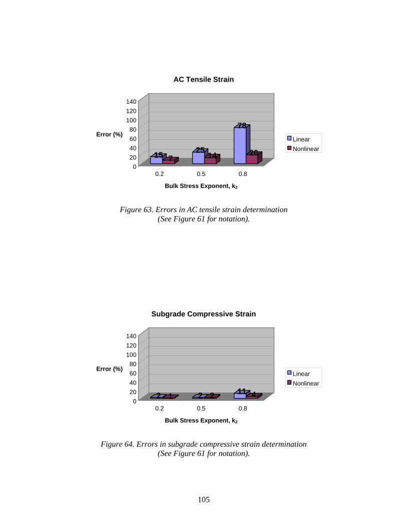
105

15 725 14

78

200

20406080

100120140

Error (%)

0.2 0.5 0.8

Bulk Stress Exponent, k2

AC Tensile Strain

LinearNonlinear

Figure 63. Errors in AC tensile strain determination

(See Figure 61 for notation).

2 1 2 2 11 40

20406080

100120140

Error (%)

0.2 0.5 0.8

Bulk Stress Exponent, k2

Subgrade Compressive Strain

LinearNonlinear

Figure 64. Errors in subgrade compressive strain determination

(See Figure 61 for notation).

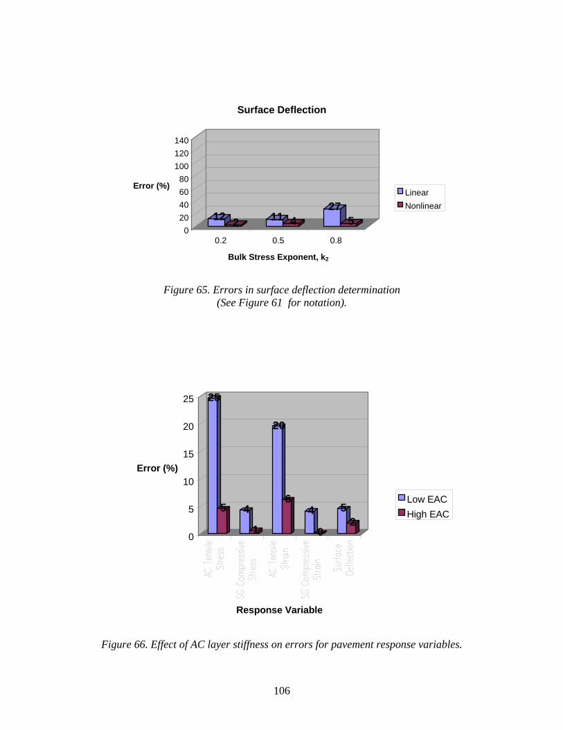
106

12 2 11 427

50

20406080

100120140

Error (%)

0.2 0.5 0.8

Bulk Stress Exponent, k2

Surface Deflection

LinearNonlinear

Figure 65. Errors in surface deflection determination

(See Figure 61 for notation).

25

5 4

1

20

64

0

52

0

5

10

15

20

25

Error (%)

Response Variable

Low EACHigh EAC

Figure 66. Effect of AC layer stiffness on errors for pavement response variables.

107

4.3 Infinite Boundary Element

The finite element analysis of pavement structures deals with an unbounded exterior domain. The simplest finite element modeling solution to such problems is to truncate the mesh at some large, but finite, distance as an approximation to “infinity.” However, this method is often expensive and inaccurate because of the large number of “extraneous” nodes and elements required to extend the boundaries to adequate distances. Another method dealing with infinite domains is through use of “infinite” elements. This solution, originally proposed by Bettess (1977), has been proven very successful and economical as well. This is the same formulation implemented in the ABAQUS general-purpose commercial finite element code.

The following sections describe the infinite boundary element formulation implemented in the DSC2D finite element program. It closely follows the derivation given in Chapter 8 of Zienkiewicz and Taylor (1989). Guidelines are also given for suitable location of the infinite boundary elements within meshes for pavement structures.

4.3.1 Finite Element Formulation

A typical geomechanics problem involving infinite domains is the excavation illustrated in Figure 67. The deformations in a semi-infinite half-space due to the removal of loads is to be determined. The far-field boundary conditions are zero displacements at infinity. The conventional approach for meshing this problem is illustrated in Figure 67a in which the infinite boundary condition is approximated by a finite boundary located at a large distance from the excavation. The obvious question, of course, is what is an adequately “large distance?” Substantial errors may arise if this boundary is not placed far enough away. On the other hand, an excessively large distance will require large number of elements to model regions of relatively little interest.

The most effective and efficient method for overcoming this problem is the use of “infinite elements” (Bettess and Zienkiewicz, 1977). As shown in Figure 67b. conventional finite elements are coupled to infinite boundary elements which model in a reasonable manner the material stretching to infinity.

The infinite element formulation is based upon mapping the element geometry and displacement fields onto a unit square (or a finite line in one dimension or cube in three dimensions) (Beer and Meek, 1981; Zienkiewicz, Emson, and Bettess, 1983). It is essential that the interpolation functions in the mapped domain be capable of modeling the true behavior as the radial distance r increases. For example, the mapped shape functions would satisfy the far field boundary conditions if they followed a sequence of the decaying form:

31 2

2 3 ...CC Cr r r

+ + + (37)

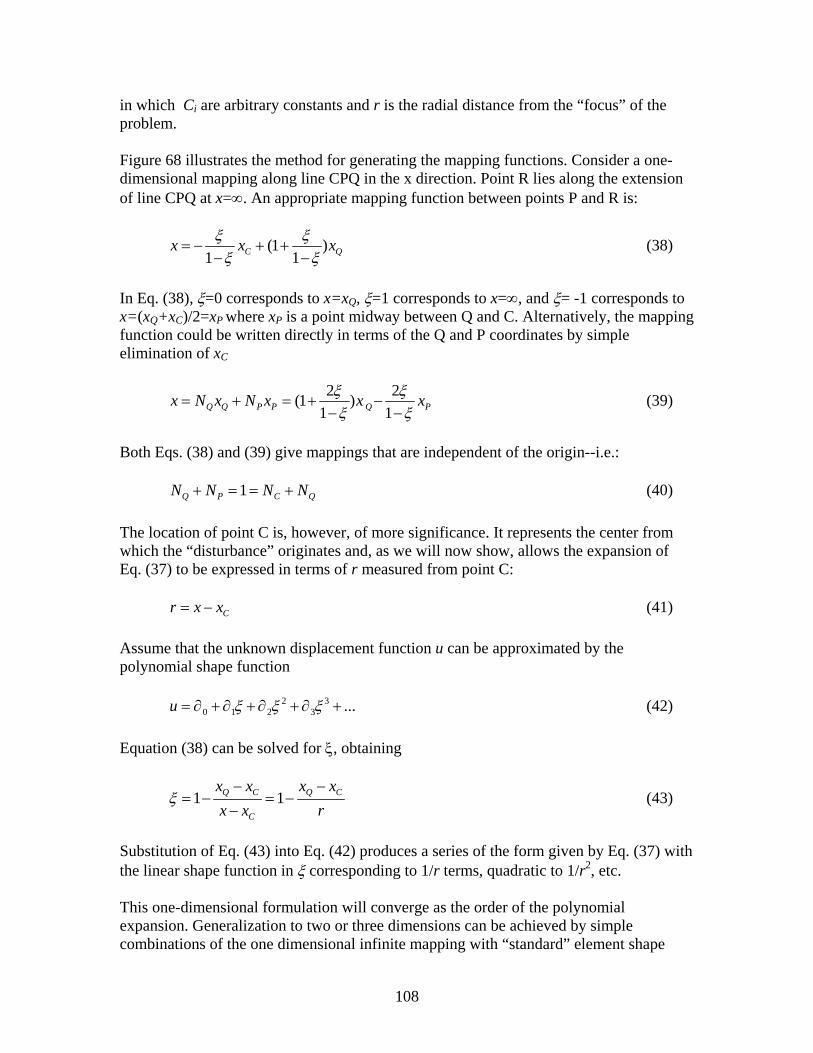
108

in which Ci are arbitrary constants and r is the radial distance from the “focus” of the problem. Figure 68 illustrates the method for generating the mapping functions. Consider a one-dimensional mapping along line CPQ in the x direction. Point R lies along the extension of line CPQ at x=∞. An appropriate mapping function between points P and R is:

(1 )1 1C Qx x xξ ξ

ξ ξ= − + +

− − (38)

In Eq. (38), ξ=0 corresponds to x=xQ, ξ=1 corresponds to x=∞, and ξ= -1 corresponds to x=(xQ+xC)/2=xP where xP is a point midway between Q and C. Alternatively, the mapping function could be written directly in terms of the Q and P coordinates by simple elimination of xC

2 2(1 )1 1Q Q P P Q Px N x N x x xξ ξ

ξ ξ= + = + −

− − (39)

Both Eqs. (38) and (39) give mappings that are independent of the origin--i.e.:

1Q P C QN N N N+ = = + (40) The location of point C is, however, of more significance. It represents the center from which the “disturbance” originates and, as we will now show, allows the expansion of Eq. (37) to be expressed in terms of r measured from point C:

Cr x x= − (41)

Assume that the unknown displacement function u can be approximated by the polynomial shape function

2 30 1 2 3 ...u ξ ξ ξ= ∂ + ∂ + ∂ + ∂ + (42)

Equation (38) can be solved for ξ, obtaining

1 1Q C Q C

C

x x x xx x r

ξ− −

= − = −−

(43)

Substitution of Eq. (43) into Eq. (42) produces a series of the form given by Eq. (37) with the linear shape function in ξ corresponding to 1/r terms, quadratic to 1/r2, etc. This one-dimensional formulation will converge as the order of the polynomial expansion. Generalization to two or three dimensions can be achieved by simple combinations of the one dimensional infinite mapping with “standard” element shape

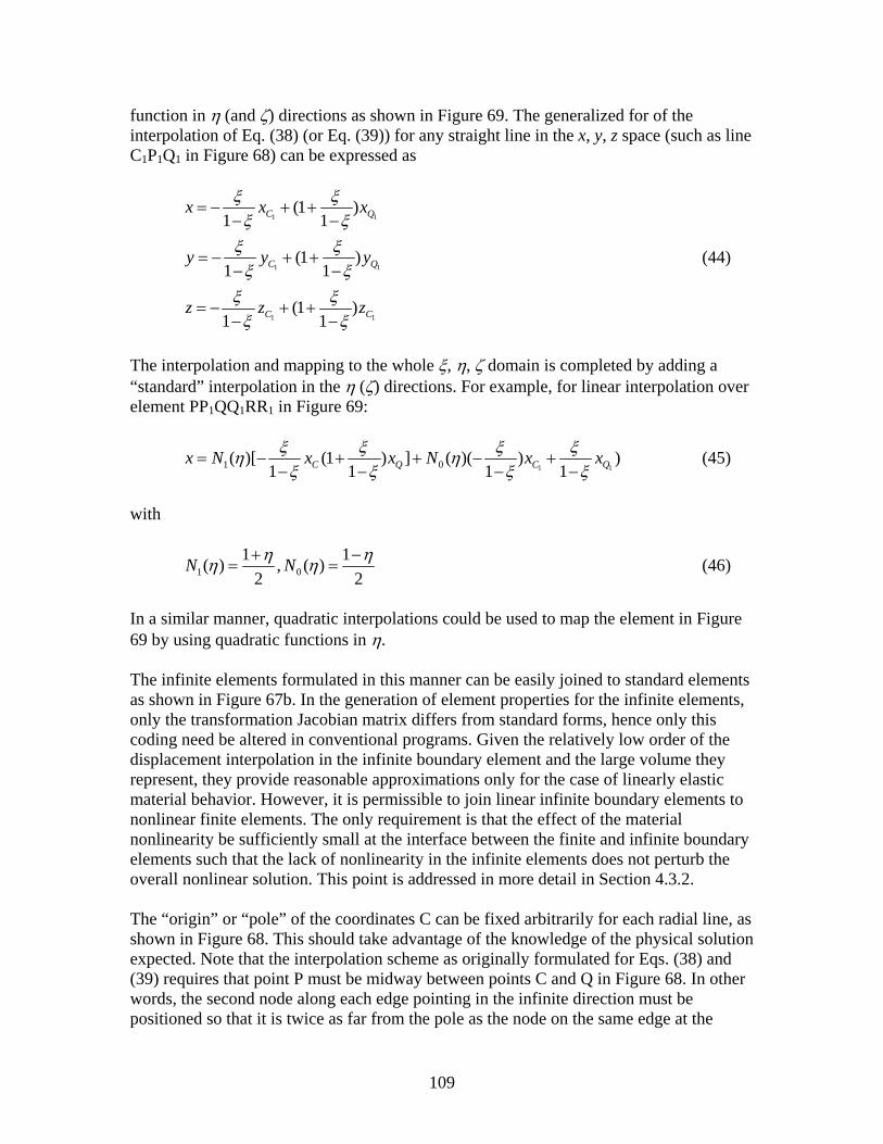
109

function in η (and ζ) directions as shown in Figure 69. The generalized for of the interpolation of Eq. (38) (or Eq. (39)) for any straight line in the x, y, z space (such as line C1P1Q1 in Figure 68) can be expressed as

1 1

1 1

1 1

(1 )1 1

(1 )1 1

(1 )1 1

C Q

C Q

C C

x x x

y y y

z z z

ξ ξξ ξ

ξ ξξ ξ

ξ ξξ ξ

= − + +− −

= − + +− −

= − + +− −

(44)

The interpolation and mapping to the whole ξ, η, ζ domain is completed by adding a “standard” interpolation in the η (ζ) directions. For example, for linear interpolation over element PP1QQ1RR1 in Figure 69:

1 11 0( )[ (1 ) ] ( )( ) )1 1 1 1C Q C Qx N x x N x xξ ξ ξ ξη η

ξ ξ ξ ξ= − + + − +

− − − − (45)

with

1 01 1( ) , ( )

2 2N Nη ηη η+ −

= = (46)

In a similar manner, quadratic interpolations could be used to map the element in Figure 69 by using quadratic functions in η. The infinite elements formulated in this manner can be easily joined to standard elements as shown in Figure 67b. In the generation of element properties for the infinite elements, only the transformation Jacobian matrix differs from standard forms, hence only this coding need be altered in conventional programs. Given the relatively low order of the displacement interpolation in the infinite boundary element and the large volume they represent, they provide reasonable approximations only for the case of linearly elastic material behavior. However, it is permissible to join linear infinite boundary elements to nonlinear finite elements. The only requirement is that the effect of the material nonlinearity be sufficiently small at the interface between the finite and infinite boundary elements such that the lack of nonlinearity in the infinite elements does not perturb the overall nonlinear solution. This point is addressed in more detail in Section 4.3.2. The “origin” or “pole” of the coordinates C can be fixed arbitrarily for each radial line, as shown in Figure 68. This should take advantage of the knowledge of the physical solution expected. Note that the interpolation scheme as originally formulated for Eqs. (38) and (39) requires that point P must be midway between points C and Q in Figure 68. In other words, the second node along each edge pointing in the infinite direction must be positioned so that it is twice as far from the pole as the node on the same edge at the

110

boundary between the finite and infinite elements. Three examples of this are shown in Figure 70 through Figure 72. In addition, the second note in the infinite direction must be specified such that the element edges in the infinite direction do not cross over, which would give nonunique mappings (see Figure 73).

Figure 67. A semi-infinite domain: soil deformations accompanying excavation.

(a) Conventional treatment. (b) Infinite element treatment. (from Zienkiewicz and Taylor, 1989)

111

Figure 68. Infinite line and element map. Linear η interpolation.

(from Zienkiewicz and Taylor, 1989)

112

Figure 69. Infinite element map. Quadratic η interpolation.

(from Zienkiewicz and Taylor, 1989)

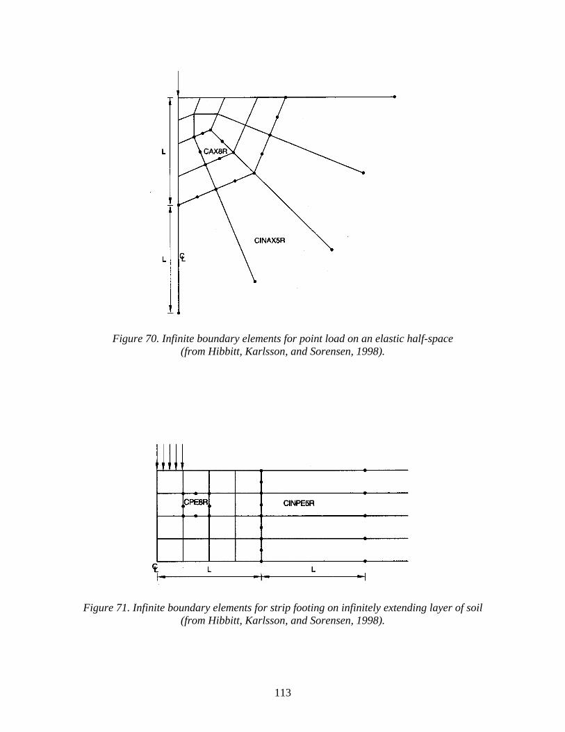
113

Figure 70. Infinite boundary elements for point load on an elastic half-space

(from Hibbitt, Karlsson, and Sorensen, 1998).

Figure 71. Infinite boundary elements for strip footing on infinitely extending layer of soil

(from Hibbitt, Karlsson, and Sorensen, 1998).

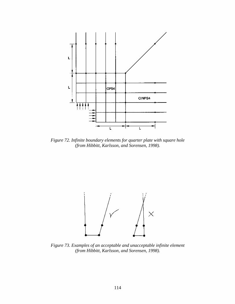
114

Figure 72. Infinite boundary elements for quarter plate with square hole

(from Hibbitt, Karlsson, and Sorensen, 1998).

Figure 73. Examples of an acceptable and unacceptable infinite element

(from Hibbitt, Karlsson, and Sorensen, 1998).

115

4.3.2 Guidelines for Infinite Boundary Element Location

As described in the preceding section, infinite boundary elements can be advantageous in reducing the size of finite element analyses for problems involving infinite or semi-infinite domains. Flexible pavement response analyses are one example of this type of problem. The infinite boundary elements should be located as close as possible to the zone of interest--i.e., the wheel loads in pavement problems--in order to maximize their benefit. If the infinite boundary elements are located too close to the zone of interest, however, they will alter the solution results and induce errors in the computed quantities. There are two potential causes for these errors. First, the infinite elements implicitly provide a lower order displacement interpolation than do the multiple finite elements they replace. Even though each individual finite element may have a low order displacement interpolation, the collection of finite elements provides a much higher effective interpolation order. This implies that the infinite boundary elements must be located sufficiently far from the zone of interest so that the displacement field is varying only gradually and can be adequately represented by the interpolation functions. Second, the infinite element formulation is based upon the assumption of linear elasticity. The elements must thus be located far enough from the zone of interest that nonlinear effects are negligible.

4.3.2.1 Location of Vertical Boundary

Parametric finite element analyses were performed to define the closest distance at which the infinite boundary elements can be located. The emphasis in this study was on the infinite boundary elements along the vertical distant boundary. The location of the infinite boundary elements along the bottom of the mesh is more straightforward to estimate (as will be discussed further in Section 4.3.2.2) and therefore this distance was kept constant in all analyses. One pavement structures was analyzed in this study, corresponding to the heavy traffic design described previously in Section 4.2.2.2 and Figure 39a. As before, the tire load is modeled as a uniform 550 kPa pressure over a circular contact area having a radius a =150 mm. The asphalt concrete and subgrade layers were modeled as conventional linearly elastic materials. Two extreme environmental variations were considered for the asphalt concrete stiffness: very cold (EAC = 12,500 MPa) and very hot (EAC = 500 MPa). The crushed stone base layer was modeled using the nonlinear resilient modulus formulation given in Eq. (8) with k6=0, k7=1, and various combinations of k1, k2, and k3. The values of k1, k2, and k3 were adjusted in each combination to produce an MR value of approximately 200 MPa under full load using mid-thickness stresses under the load centerline as computed from the KENLAYER MLET program (w/ Ebase = 200 MPa). The material properties used in the parametric analyses are summarized in Table 16. All calculations were performed using the DSC2D finite element program. The finite element meshes took advantage of the axial symmetry of the problem. Nine meshes were constructed in order to determine the closest distance at which the infinite boundary elements along the vertical boundary can be located. As shown schematically in Figure

116

74, the infinite boundary elements were located at a distance Lb from the centerline of the tire load, and Lb was varied between 2a and 10a. The infinite boundary elements along the lower boundary of the mesh (i.e., within the subgrade) were located at a depth of 350 mm for the low traffic pavement structure and 725 mm for the high traffic design. The rule of thumb frequently stated in the literature for the location of the distant vertical mesh boundaries when infinite boundary elements are not used is approximately 20a. Finite element meshes for these conditions were also prepared and analyzed. Experience shows that this distance is sufficient to approximate the infinite domain in pavement problems when infinite boundary elements are not employed. The distance to the infinite boundary elements is judged to be too close when the solution with the infinite elements begins to deviate significantly from the solution without (i.e., the solution with the vertical boundary at a horizontal distance of 20 tire radii from the load centerline). The solution parameters evaluated in this study were:

• the horizontal tensile stress at the bottom of the asphalt layer • the horizontal tensile strain at the bottom of the asphalt layer • The vertical compressive stress at the middle of the base layer • the vertical compressive strain at the middle of the base layer • the vertical compressive stress at the top of the subgrade • the vertical compressive strain at the top of the subgrade

Figure 76 through Figure 81 show the variations of these quantities as a function Lb/a, the normalized radial distance from the center of the load to the infinite elements along the distant vertical boundary. In each figure, the upper portion (a) is for the soft asphalt condition (EAC = 500 MPa) and the lower portion (b) is for the stiff asphalt case (EAC = 12,500 MPa). The pavement response quantities are expressed in normalized form:

Response w/ Infinite Elements @ /Response Ratio = Response w/out Infinite Elements, Boundary @ 20

bL aa

(47)

The results in Figure 76 through Figure 81 are remarkably consistent. The normalized pavement response ratios approach a value of 1 (i.e., no perturbation of solution due to infinite boundary elements) as Lb/a increases, as expected. However, in all cases and for all response quantities, the deviation of the normalized response ratio from a value of 1 becomes insignificantly small for Lb/a greater than about 7. The results from any parametric study are always limited. However, the results from the cases considered here are intuitively reasonable and very consistent. The conclusion from these results is that the horizontal distance from the center of the loading to the infinite elements along the distant vertical boundary should be at least 7 times the effective loading radius.

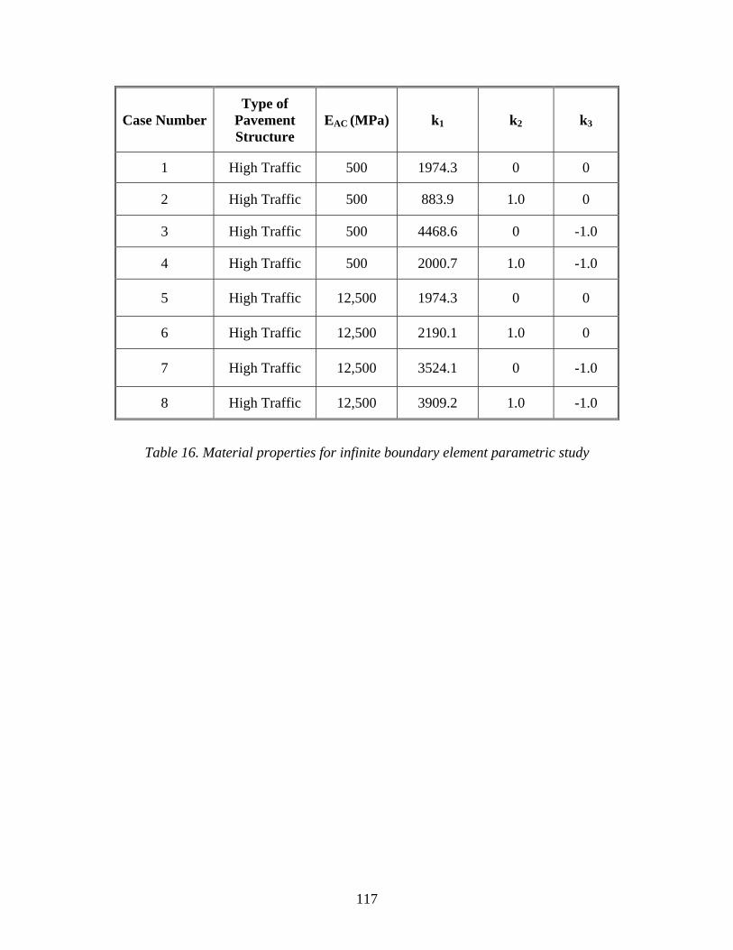
117

Case Number Type of

Pavement Structure

EAC (MPa) k1 k2 k3

1 High Traffic 500 1974.3 0 0

2 High Traffic 500 883.9 1.0 0

3 High Traffic 500 4468.6 0 -1.0

4 High Traffic 500 2000.7 1.0 -1.0

5 High Traffic 12,500 1974.3 0 0

6 High Traffic 12,500 2190.1 1.0 0

7 High Traffic 12,500 3524.1 0 -1.0

8 High Traffic 12,500 3909.2 1.0 -1.0

Table 16. Material properties for infinite boundary element parametric study

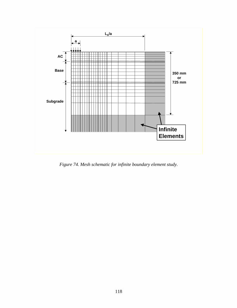
118

350 mmor

725 mm

a

Lb/a

AC

Base

Subgrade

Infinite Elements

Figure 74. Mesh schematic for infinite boundary element study.

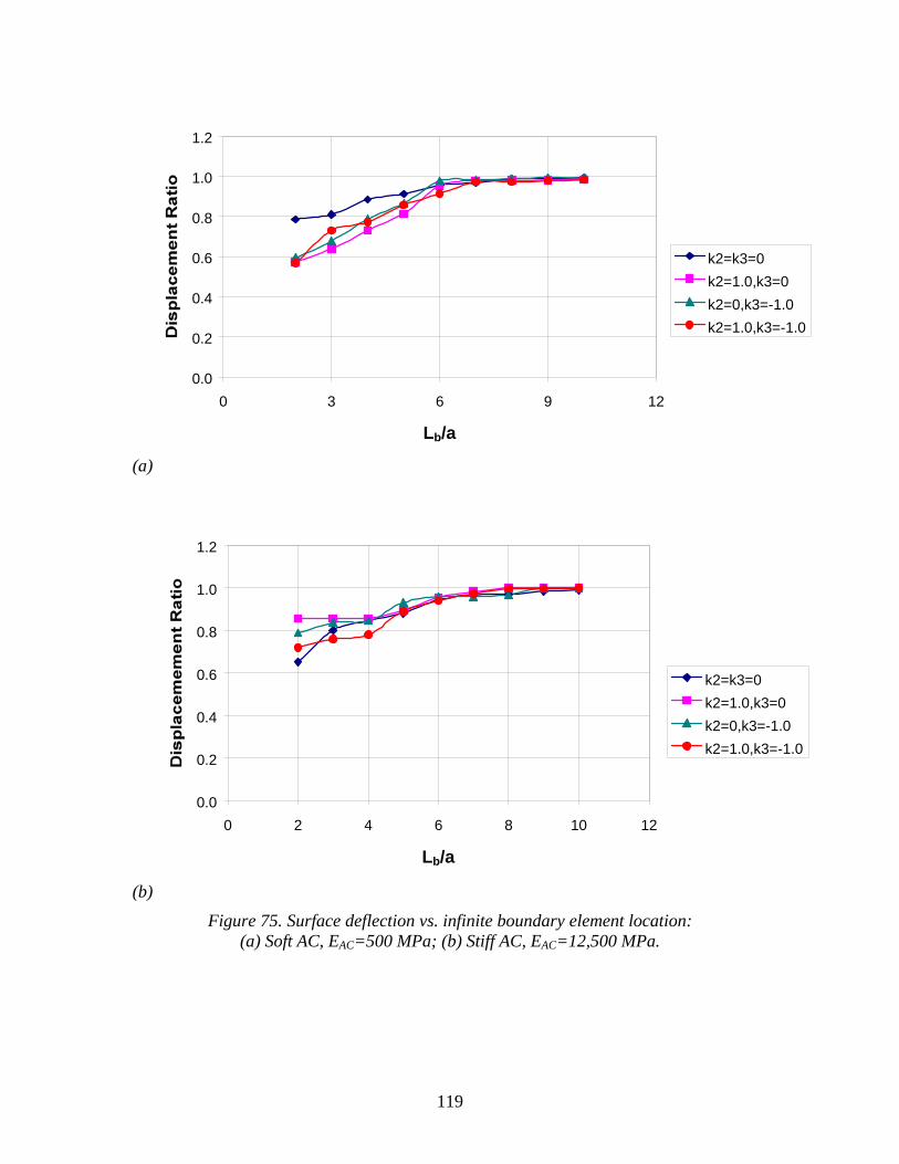
119

0.0

0.2

0.4

0.6

0.8

1.0

1.2

0 3 6 9 12

Lb/a

k2=k3=0k2=1.0,k3=0k2=0,k3=-1.0k2=1.0,k3=-1.0

(a)

0.0

0.2

0.4

0.6

0.8

1.0

1.2

0 2 4 6 8 10 12

Lb/a

k2=k3=0k2=1.0,k3=0k2=0,k3=-1.0k2=1.0,k3=-1.0

(b)

Figure 75. Surface deflection vs. infinite boundary element location: (a) Soft AC, EAC=500 MPa; (b) Stiff AC, EAC=12,500 MPa.

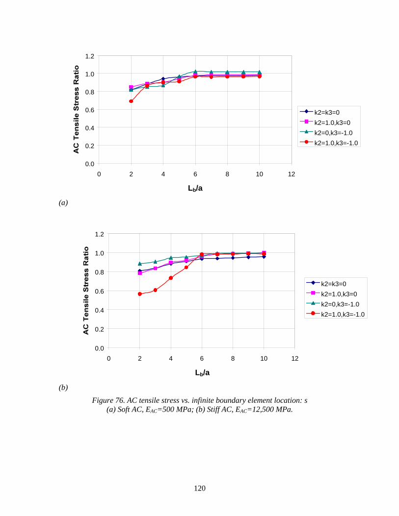
120

0.0

0.2

0.4

0.6

0.8

1.0

1.2

0 2 4 6 8 10 12

Lb/a

k2=k3=0k2=1.0,k3=0k2=0,k3=-1.0k2=1.0,k3=-1.0

(a)

0.0

0.2

0.4

0.6

0.8

1.0

1.2

0 2 4 6 8 10 12

Lb/a

k2=k3=0k2=1.0,k3=0k2=0,k3=-1.0k2=1.0,k3=-1.0

(b)

Figure 76. AC tensile stress vs. infinite boundary element location: s (a) Soft AC, EAC=500 MPa; (b) Stiff AC, EAC=12,500 MPa.

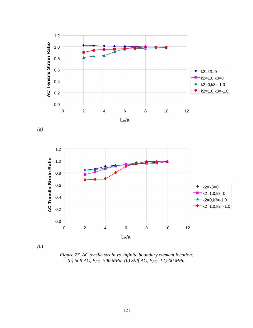
121

0.0

0.2

0.4

0.6

0.8

1.0

1.2

0 2 4 6 8 10 12

Lb/a

k2=k3=0k2=1.0,k3=0k2=0,k3=-1.0k2=1.0,k3=-1.0

(a)

0.0

0.2

0.4

0.6

0.8

1.0

1.2

0 2 4 6 8 10 12

Lb/a

k2=k3=0k2=1.0,k3=0k2=0,k3=-1.0k2=1.0,k3=-1.0

(b)

Figure 77. AC tensile strain vs. infinite boundary element location: (a) Soft AC, EAC=500 MPa; (b) Stiff AC, EAC=12,500 MPa.

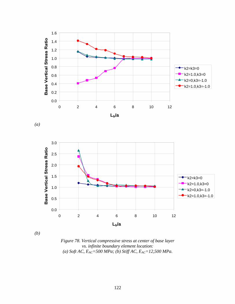
122

0.0

0.2

0.4

0.6

0.8

1.0

1.2

1.4

1.6

0 2 4 6 8 10 12

Lb/a

k2=k3=0k2=1.0,k3=0k2=0,k3=-1.0k2=1.0,k3=-1.0

(a)

0.0

0.5

1.0

1.5

2.0

2.5

3.0

0 2 4 6 8 10 12

Lb/a

k2=k3=0k2=1.0,k3=0k2=0,k3=-1.0k2=1.0,k3=-1.0

(b)

Figure 78. Vertical compressive stress at center of base layer vs. infinite boundary element location:

(a) Soft AC, EAC=500 MPa; (b) Stiff AC, EAC=12,500 MPa.

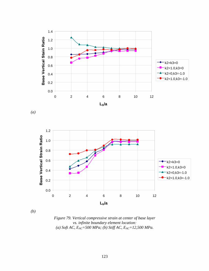
123

0.0

0.2

0.4

0.6

0.8

1.0

1.2

1.4

0 2 4 6 8 10 12

Lb/a

k2=k3=0k2=1.0,k3=0k2=0,k3=-1.0k2=1.0,k3=-1.0

(a)

0.0

0.2

0.4

0.6

0.8

1.0

1.2

0 2 4 6 8 10 12

Lb/a

k2=k3=0k2=1.0,k3=0k2=0,k3=-1.0k2=1.0,k3=-1.0

(b)

Figure 79. Vertical compressive strain at center of base layer vs. infinite boundary element location:

(a) Soft AC, EAC=500 MPa; (b) Stiff AC, EAC=12,500 MPa.

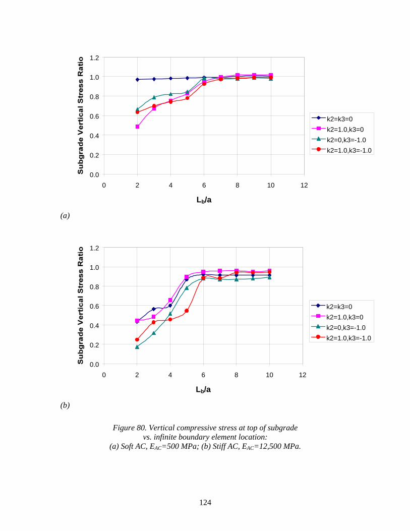
124

0.0

0.2

0.4

0.6

0.8

1.0

1.2

0 2 4 6 8 10 12

Lb/a

k2=k3=0k2=1.0,k3=0k2=0,k3=-1.0k2=1.0,k3=-1.0

(a)

0.0

0.2

0.4

0.6

0.8

1.0

1.2

0 2 4 6 8 10 12

Lb/a

k2=k3=0k2=1.0,k3=0k2=0,k3=-1.0k2=1.0,k3=-1.0

(b)

Figure 80. Vertical compressive stress at top of subgrade vs. infinite boundary element location:

(a) Soft AC, EAC=500 MPa; (b) Stiff AC, EAC=12,500 MPa.

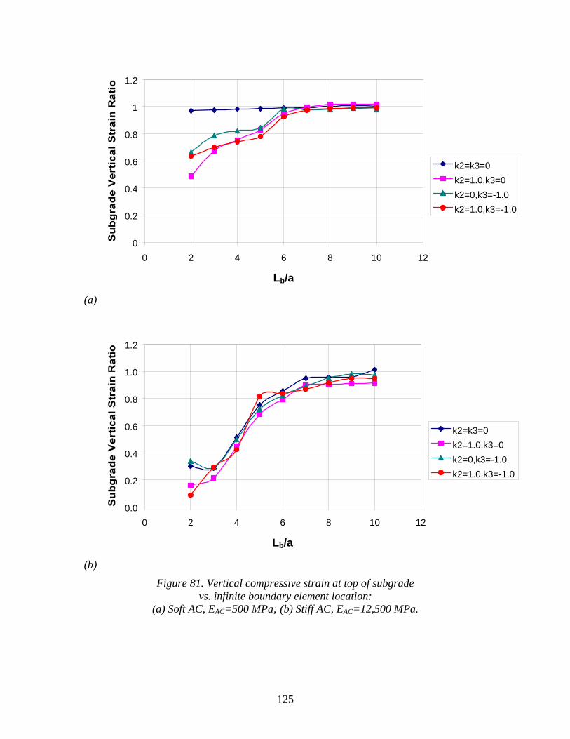
125

0

0.2

0.4

0.6

0.8

1

1.2

0 2 4 6 8 10 12

Lb/a

k2=k3=0k2=1.0,k3=0k2=0,k3=-1.0k2=1.0,k3=-1.0

(a)

0.0

0.2

0.4

0.6

0.8

1.0

1.2

0 2 4 6 8 10 12

Lb/a

k2=k3=0k2=1.0,k3=0k2=0,k3=-1.0k2=1.0,k3=-1.0

(b)

Figure 81. Vertical compressive strain at top of subgrade vs. infinite boundary element location:

(a) Soft AC, EAC=500 MPa; (b) Stiff AC, EAC=12,500 MPa.

126

4.3.2.2 Location of Horizontal Boundary

A conservative estimate of the minimum vertical distance from the pavement surface to the infinite elements along the distant lower vertical boundary of the finite element mesh (i.e., the “bottom” of the subgrade) can be based on the following argument: The lower infinite boundary elements should be located at or below the depth at which the maximum induced vertical stress in the subgrade becomes insignificantly small--e.g., 1% or less of the applied tire pressure.

A well-designed pavement is intended to protect the subgrade, i.e., to lower the induced stresses in the subgrade. Therefore, the conventional Boussinesq solution for the stresses beneath a circular uniform pressure on an isotropic homogeneous soil mass is an upper bound for the actual induced stresses in the subgrade beneath a layered pavement structure. The well-known Boussinesq solution for the induced vertical stresses beneath the center of the circular loaded are is

( )

3/ 22

1/ 1/ 1

v pa z

∆σ = −⎡ ⎤+⎣ ⎦

(48)

in which z is the depth beneath the surface, a is the tire radius, and p is the tire pressure. Table 17 shows values of ∆σv / p vs. z for typical pavement conditions under a single wheel load (a ≅ 6 inches). Given that the Boussinesq solution provides an upper bound for the induced vertical subgrade stresses in a layered pavement system, the values in Table 17 suggest that a distance of 36 to 50 inches to the lower infinite boundary elements should be sufficient.

∆σv / p Depth (inches)0.10 24 0.05 36 0.02 50 0.01 75

Table 17. Vertical stress attenuation vs. distance for Boussinesq circular load solution.

127

5. PRE-DSC PREPROCESSOR PROGRAM

As mentioned previously, one of the disadvantages of the finite element method is the large volume of required input data. The problem domain must be divided into hundreds or thousands of small rectangular elements that are defined in terms of the coordinates of their corners, termed “nodes.” Input data required for the analysis consists of the coordinates for each node, the connectivity for each element (i.e., the node identifiers for each of the corners), the material properties for each layer (adjusted for seasonal influences, as necessary), and the tire loads (again defined in terms of loads at node points). This translates to thousands of data records for a typical pavement analysis. Output data from the finite element analysis is equally voluminous. Unlike MLET in which output is obtained only for the discrete points at which it is requested, finite element programs by default generate displacements for every node and stresses and strains for every element (often at multiple locations within each element) for each load condition. This also translates to thousands of data records for a typical pavement analysis. Interactive pre- and post-processors are generally used to aid in the processing of this voluminous information. In the 2002 Design Guide flexible pavement module, specialized pre- and post-processors have been developed to shield the user from the details of the finite element data. PRE-DSC is the pre-processor program for converting analysis control information generated by the 2002 Design Guide user interface program into an appropriate format for input to the DSC2D finite element program. PRE-DSC contains the finite element mesh generator for modeling the layered pavement structure, loads, and boundary conditions. Generation of the finite element mesh is the major component in PRE-DSC. All meshes are generated using 4-node quadrilateral elements, 4-node interface elements, and infinite boundary elements. Some of the rules governing this mesh generation are: • Axially symmetric boundary conditions. • Up to 75 layers (see Figure 82a; this can be increased if necessary). • Infinite boundary elements at appropriate distances (rMax, zMax) from the tire load

(see Figure 82a). • A minimum of nrElts elements beneath the tire contact radius (see Figure 82b). • A minimum of nEltUniform blocks of approximately uniform elements in the region

of interest immediately beneath the wheel load (see Figure 82b). • A minimum of nEltMin elements through the thickness of any individual layer (see

Figure 82b). • An element aspect ratio of approximately 1:1 in regions of the mesh close to the tire

load—i.e., in the areas of high stress and strain gradients layer (see Figure 82b). • Growth in element aspect ratio by factor of xRatio to a maximum aspect ratio of

aspectMax in regions of the mesh remote from the wheel load—i.e., in the areas of low stress and strain gradients layer (see Figure 82b).

128

• Option for interface layers between each pair of adjacent layers (thickInterface in Figure 82b); the interface condition can range from full shear transfer to zero shear transfer.

These rules are designed to produce finite element models having adequate solution accuracy and minimum computational time. The input and output data files for PRE-DSC are described separately in Section 7 of this appendix.

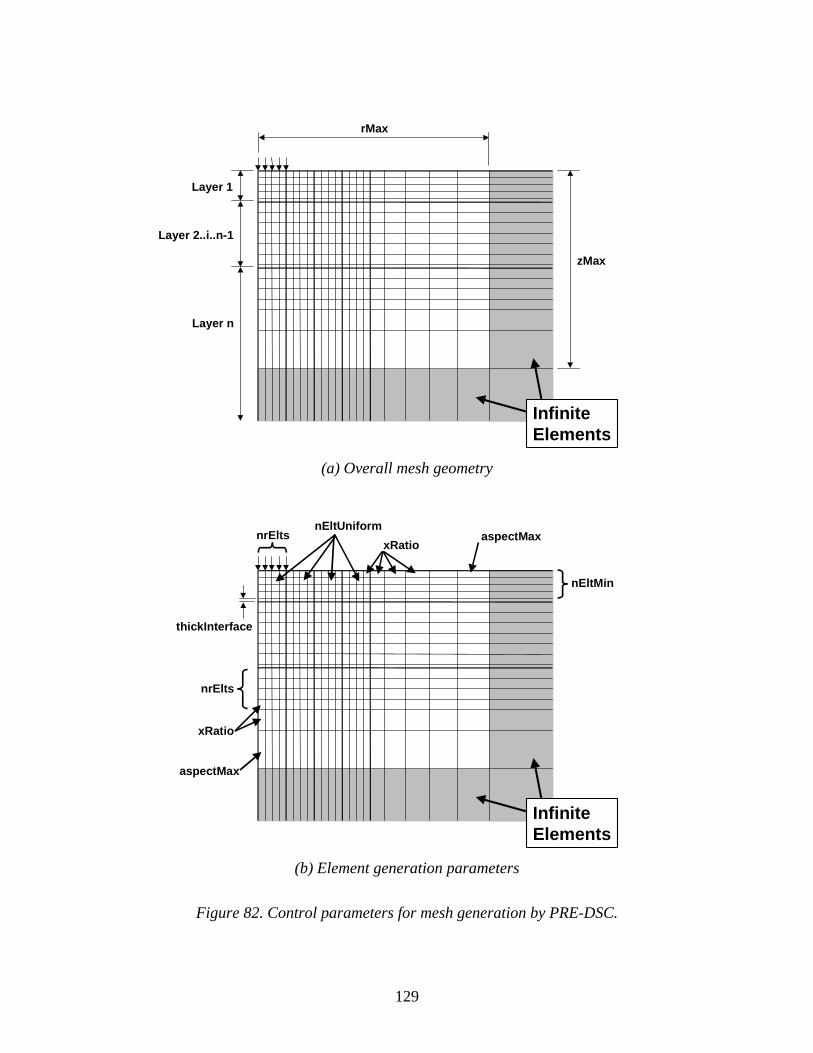
129

rMax

Layer 1

Layer 2..i..n-1

Layer n

Infinite Elements

zMax

(a) Overall mesh geometry

Infinite Elements

nrEltsnEltUniform

nEltMin

thickInterface

xRatioaspectMax

xRatio

aspectMax

nrElts

(b) Element generation parameters

Figure 82. Control parameters for mesh generation by PRE-DSC.

130

6. POST-DSC POSTPROCESSING PROGRAM

POST-DSC is the post-processor program for converting the stress and strain data output from the DSC2D-DSC finite element program into an appropriate format for return to the 2002 Design Guide flexible pavement module for use in pavement damage and performance prediction. POST-DSC contains the logic for superimposing the single wheel solutions generated by DSC2D into the appropriate multi-wheel solutions for single, tandem, tridem, and quad axles. The superimposed stress and strain values at the potentially critical locations in the pavement are then passed back to the 2002 Design Guide user interface program for use in the pavement damage and performance prediction models. The input and output data files for POST-DSC are described separately in Section 7 of this appendix.

x

y

8 in 8 in 8 inSx

Sy

CL

A1 A2 A3 A4 A5 A6 A7 A8 A9 A10

B1 B2 B3 B4 B5 B6 B7 B8 B9 B10

4 in4 in

Figure 83. Plan view of calculation points for general traffic loading.

131

7. PROGRAM INPUT/OUTPUT FILES

7.1 Overview

All data required by the finite element programs in the 2002 Design Guide are passed via files. The following subsections list the input and output files used by the PRE, DSC2D, and POST programs. Detailed file formats for each of these files are described subsequently in Sections 7.2 through 7.4.

7.1.1 PRE Pre-Processor Program

Input Files:

File Name Description Where Generatedlayers.csv Pavement structure for each analysis

period over entire analysis duration. 2002 Design Guide User Interface program

layers.ini Control parameters Pre-defined LoadLevels.csv Wheel loads (lbs) for each axle category

and load group. Pre-defined

project_SingleAxleOutput.csv Axle load spectrum for single axle category (standard traffic option only)

Traffic Module

project_TandemAxleOutput.csv Axle load spectrum for tandem axle category (standard traffic option only)

Traffic Module

project_TridemAxleOutput.csv Axle load spectrum for tridem axle category (standard traffic option only)

Traffic Module

project_QuadAxleOutput.csv Axle load spectrum for quad axle category (standard traffic option only)

Traffic Module

project_GeneralOutput.csv Load control information (standard traffic option only)

Traffic Module

UserTraffic.csv User-defined axle load configuration (for user-defined gear option only; actual file name is generated by the 2002 Design Guide User Interface program)

2002 Design Guide User Interface program

Output Files:

File Name Description pre.log PRE log file (error messages, etc.) prepost.dat Control data input for POST dsc.in1 Input data for DSC2D finite element analysis program (Part 1) dsc.in2 Input data for DSC2D finite element analysis program (Part 2)

132

7.1.2 DSC2D Finite Element Program

Input Files:

File Name Description Where Generateddsc.in1 Input data for finite element analysis

(Part 1) PRE

dsc.in2 Input data for finite element analysis (Part 2)

PRE

Output Files:

File Name Description dsc2d.log DSC2D log file (error messages, etc.) for.tmp Temporary storage file emmmm-nn.out Element stresses and strains for analysis period mmmm and load level nn

(Note: For binary output option (default set in code), nn equals 1 always and the file contains in sequence the results for all load levels for analysis period mmmm.)

Supplementary Output Files (if IPRINT=.TRUE. in code):

File Name Description dsc.out Print output file dsc.dsp Nodal displacements dsc.str Nodal stresses

7.1.3 POST Post-Processor Program

Input Files:

File Name Description Where Generatedprepost.dat Control data PRE emmmm-nn.out Element stresses and strains for analysis period

mmmm and load level nn DSC2D

Output Files:

File Name Description post.log POST log file (error messages, etc.) permdef.out Stress and strain data for permanent deformation model fatigue.out Strain data for fatigue model

133

7.2 PRE Input/Output Files

LAYERS.CSV

This is the main input file to the finite element preprocessor program PRE. It describes the pavement layer structure for each analysis period in the design. It must be generated by the main 2002 Design Guide User Interface program. LAYERS.CSV is in ASCII text format. The input data for LAYERS.CSV are organized into record groups. Records may be repeated within a group. Multiple data values in a single record may be entered in either comma- or space-delimited format. File Structure: Record Group/Description Variable 1. Project name (as used as prefix on traffic files)1 Project1 2. Tire radius (inches)2 Radius2 3. Traffic code: 0=general traffic, 1=user-defined traffic TrafficCode 4. File name for user-defined traffic. (Omit if TrafficCode=0)3

TrafficFileName3 5. Total number of layers4 NL4 6. Constant Layer Properties (repeat for NL layers)

Layer number IL Material category Matcat

0=asphalt 1=bedrock 2=cementitiously stabilized 3=unbound base/subbase 4=PCC 5=compacted SG 6=uncompacted SG

Layer thickness (inches)5 Thick5

Material unit weight for layer (pcf) Gamma Lateral in situ stress ratio for layer K0 Interface condition at bottom of layer6 Friction6

0 (full slip) < Friction < 1 (full friction) 7. Analysis Season Identification (one record)

Analysis year (e.g., 2000) Year Analysis month (season—e.g., July; limit of 10 characters) Month 0 for whole month, 1 for half-month MonthCode 1 for whole month/first half of month, 2 for second half Submonth Analysis subseason (e.g., 1) Subseason

134

8. Seasonally Varying Layer Properties (repeat for NL layers) Layer number IL Material type for layer: 1 = linearly elastic, 7 = nonlinear MR Mattyp Elastic modulus (psi) (for Mattyp=1)4 Emod Poisson’s ratio (for all Mattyp) Vnu Nonlinear modulus parameter k1 (for Mattyp=7)7 K17

(pa implicitly in psi) Nonlinear modulus parameter k2 (for Mattyp=7)7 K27

Nonlinear modulus parameter k3 (for Mattyp=7)7 K37

Environmental reduction factor for K17 RF7 (repeat Records Groups 7-8 for all analysis periods) Notes: 1Must be enclosed within single quotes if contains embedded spaces (e.g., ‘Test Project’). 2Assumed constant for all wheels throughout analysis. 3Enclose file name in single quotes (‘ ‘) as appropriate. 4Maximum number of layers is 25, but this can be increased in necessary. 5For infinite subgrade, specify Thick > 999 for lowest layer. 6Ignored for bottom layer; enter 1.0 for this case. 7Ignored for other Mattyp; enter 0.0 in this case.

135

LAYERS.INI

Default initialization/control parameters for PRE pre-processor program. LAYERS.INI is in ASCII text file format. File Structure: Record/Description Variable 1. Distance to radial mesh boundary (inches) rMax1 2. Distance to lower mesh boundary (inches) zMax2 3. Number of elements across tire radius at surface nrElts3 4. Number of blocks of nrElts in r-direction nEltUniform 5. Minimum number of elements per layer nEltMin3 6. Growth ratio for element dimensions xRatio 7. Maximum element aspect ratio aspectMax 8. Thickness for interface elements (inches) thickInterface 9. Modulus for interface elements (psi) Einterface 10. Minimum value for interface friction parameter minFriction 11. Unit weight of water (pci) rowat 12. Atmospheric pressure (psi) atmc 13. Threshold RF value, above which soil is assumed frozen RFfrozen 14. Elastic modulus for frozen soil (psi) Efrozen 15. Minimum tangent modulus for nonlinear Mr (psi) Etmin 16. Maximum tangent modulus for nonlinear Mr (psi) Etmax 17. Iteration acceleration parameter for nonlinear Mr alpha 18. Number of iterations niter 19. Integration order (0=2 point, 1=3 point) nint 20. Maximum load step size (psi) stepSize Notes: 1May be adjusted internally by the program based on the particular problem characteristics based on the algorithm:

rMax = max( rMax, 8*radius, 1.2*rcMax ) in which radius is the tire radius and rcMax is the longest horizontal distance between any tire and any calculation point. 2May be adjusted internally by the program based on the particular problem characteristics based on the following algorithm: zMax = max( zMax, 12.5*radius, thickAboveSG+36)

136

in which radius is the tire radius and thickAboveSG is the total thickness of all layers above the top of the subgrade. 3May be adjusted internally by the program based on the particular problem characteristics such that the element aspect ratios are always less than aspectMax.

137

LOADLEVELS.CSV

This is a supplementary input file to the finite element preprocessor program PRE. It contains information on the tire loads for each standard load level in each axle category. It is in ASCII text file format and is predefined. File Structure: Record Group/Description Variable 1. Load Group Data (repeat for 70 load groups)

Load group number for single axles I1 Load group number for tandem axles I2

Load group number for tridem axles I3 Load group number for quad axles I4

Tire load index I5 Tire load (lbs) TIRELOAD

138

PREPOST.DAT

Control data generated by the PRE pre-processor program for use by the POST post-processor. PREPOST.DAT is in ASCII text file format. File Structure: Record/Description Variable 1. Project name (as used as prefix on traffic files)1 Project1 2. Tire radius (inches)2 Radius2 3. Traffic code: 0=general traffic, 1=user-defined traffic TrafficCode 4. Number of vehicle/axle group types nvtypes 5. Tire coordinates (repeat for nvtypes sets):

Number of tires for vehicle/axle group i ntires(i) x, z plan coordinates for tire j (repeat for ntires(i) sets) xw(j),zw(j)3

Number of calculation line longitudinal offsets for vehicle/axle group i nzoff(i)3

Offset coordinate for calculation line j (repeat for nzoff(i) offsets) zoff(j)3

6. Transverse offsets for calculation points (10 values on one record) xoff(i),i=1,103 7. Mesh Generation Data (one record)

Number of layers nl Distance to far vertical mesh boundary rMax Distance to lower mesh boundary zMax Number of node points in radial direction per layer nrPts Number of node points in the vertical direction per column nzPts Total number of nodal points nnp Total number of elements nel

8. Layer Property Data (nl records) Material category for layer matcat(i)

0=asphalt 1=bedrock 2=cementitiously stabilized 3=unbound base/subbase 4=PCC 5=compacted SG 6=uncompacted SG

Layer thickness thick(i) Interface friction coefficient at bottom of layer friction(i) Number of element layers in this pavement layer nEltLayers(i)

9. Element Centroid Coordinates (nel records) Element number i Radial coordinate of element centroid rc Vertical coordinate of element centroid yc

139

10. Analysis Season Identification (one record) Analysis year (e.g., 2000) year Analysis month (season—e.g., July; limit of 10 characters) month 0 for whole month, 1 for half-month MonthCode 1 for whole month/first half of month, 2 for second half Submonth Analysis subseason (e.g., 1) subseason

11. Number of load increments nincr 12. Load Increment Mapping Data (nincr records)

Load group for this increment for single axle vehicles loadType(i,1) Load group for this increment for tandem axle vehicles loadType(i,2) Load group for this increment for tridem axle vehicles loadType(i,3) Load group for this increment for quad axle vehicles loadType(i,4)

Notes: 1Output enclosed within single quotes (e.g., ‘Test Project’). 2Assumed constant for all wheels throughout analysis. 3The longitudinal plan direction corresponds to the vehicle centerline. The transverse plan direction is parallel to the vehicle axles.

140

PROJECT_SINGLEAXLEOUTPUT.CSV

PROJECT_TANDEMAXLEOUTPUT.CSV

PROJECT_TRIDEMAXLEOUTPUT.CSV

PROJECT_QUADAXLEOUTPUT.CSV

PROJECT_GENERALOUTPUT.CSV

Axle load spectrum data. See separate documentation for Traffic Module.

141

USERTRAFFIC.CSV

Axle/wheel configuration for user-defined vehicle option. Actual file name is generated by the 2002 Pavement Design Guide User Interface program and passed to the finite element routines via the LAYERS.CSV input file. USERTRAFFIC.CSV is in ASCII text file format. The input data are organized into record groups. Records may be repeated within a group. Multiple data values in a single record may be entered in either comma- or space-delimited format. File Structure: Record/Description Variable 1-9 (not used by PRE program; skip) 10. Maximum tire pressure (psi) maxpressure 11. Tire contact radius (in) radius1 12. Number of tires for vehicle ntires 13. x, z plan coordinates for tire j (repeat for ntires sets) xw(j),zw(j)2 14. Number of calculation line longitudinal offsets nzoff2 15. Offset coordinate for calculation line j (repeat for nzoff offsets) zoff(j)2 16. Transverse offsets for calculation points (10 values on one record) xoff(i),i=1,102 Notes: 1This value for radius overrides the value specified in layers.csv. 2The longitudinal plan direction corresponds to the vehicle centerline. The transverse plan direction is parallel to the vehicle axles.

142

7.3 DSC2D Input/Output Files

The main input files for the DSC2D finite element program are DSC.IN1 and DSC.IN2. DSC.IN1 contains the portion of the finite element input data that varies from one analysis period to the next (e.g., layer properties, traffic loads), while DSC.IN2 contains the portion of the finite element input data that remains constant across all analysis periods (e.g., mesh geometry). The DSC.IN1 and DSC.IN2 files are in ASCII text format. The input data in each file are organized into record groups. Records may be repeated within a group. Multiple data values in a single record may be entered in either comma- or space-delimited format. Note that the DSC2D program was originally designed for analyses other than pavements and therefore includes features that are not used in the 2002 Pavement Design Guide application. In the interests of completeness, however, all input features are documented here, and those that are not used for the 2002 Pavement Design Guide analyses are indicated. The sign convention for stresses and strains in DSC2D is compression positive, the usual case for geomechanics analyses. The y-coordinate direction is axial (vertical), and the x-coordinate direction is radial (horizontal).

143

DSC.IN1

DSC.IN1 contains the portion of the finite element input data that changes from one analysis period to the next. File Structure: Record Group/Description Variable 1. Title of the problem (single record) TITLE

(Note: For the 2002 Pavement Design Guide, TITLE contains the concatenated Year, Month, MonthCode, Submonth, Subseason codes from LAYERS.CSV)

2. Material Properties (repeat for NMAT materials) Constitutive model JCODE 1 = Linear elastic 2 = Variable modulus (not used here) 3 = Drucker-Prager (not used here) 4 = Critical state (not used here) 5 = Interface 6 = Cap model (not used here) 7 = Nonlinear resilient modulus Element type IELTYP 1 = Soil1 2 = Structure1 5 = Infinite elements along vertical sides (pavement analyses) 6 = Infinite elements along horizontal base (pavement analyses) Young’s modulus (initial)2 E2 Poisson’s ratio PR Unit weight3 ROSOIL3 Coefficient of lateral earth pressure (Ko)3 COER3 Material property values (see Table 18 for definitions) PROP(1)

: PROP(2) : PROP(3) : PROP(4)

: PROP(5) : PROP(6)

: PROP(7) : PROP(8) : PROP(9) : PROP(10)

144

Notes: 1For soil elements (i.e., IELTYP=1), a reduced modulus is used to simulate a tension cut-off for all material models other than the nonlinear resilient modulus model (i.e., all models other than JCODE=7). In these cases, the material at an integration point is treated as linearly elastic with Eanalysis=0.0001Einput whenever one of the in-plane normal stresses is nonpositive. The tension cut-off is implemented slightly differently for the nonlinear resilient modulus model (JCODE=7); details are documented elsewhere. For all element types other than soil elements (i.e., IELTYP<>1), no tension cut-off algorithm is applied. 2Not used for the nonlinear resilient modulus model (JCODE=7). 3Used only for in situ stress calculations for soil analyses. Not used for pavement analyses in the 2002 Pavement Design Guide; see record group 5 instead.

3. Load Cases (single record)

Load case type NSEQ1

1 = in situ stresses1 2 = uniform field stresses 3 = surface point loads Number of surface load records2 NSLC2

Number of concentrated load records3 NFORCE3

Number of load increments for this load case4 NSTEP4

Notes: 1If NSEQ=1, the program evaluates the initial stresses from an elastic analysis using ROSOIL and sets σx=Koσy, τxy=0 (based on a horizontal surface). For use in the 2002 Pavement Design Guide, NSEQ=3 always. 2For the example in Figure 7, NSLC=1. 3For the example in Figure 7, NFORCE=1. 4NSTEP is the number of equal load subincrements into which the load case is divided for nonlinear analyses. For linear analyses, set NSTEP=1.

4. Uniform Field Stress Loads1 (Skip if NSEQ ≠ 2; otherwise provide single record.)

Hydrostatic pressure PRE Initial void ratio VODO Hardening parameter po PO Note:

1This allows application of uniform initial stress field conditions and is also used for the Critical State constitutive model. Omit this record for the 2002 Pavement Design Guide application.

145

5. Surface Loads (Skip if NSLC=0; otherwise, provide NSLC records. See Figure 84 for notation.)

Node I ISC Node J JSC Node K KSC Stress in x-direction at node I STXI Stress in x-direction at node K STXK Stress in y-direction at node I STYI Stress in y-direction at node K STYK Note: For the example in Figure 7, ISC=19, JSC=18, KSC=17, STXI=STXK=0, and STYI=STYK=TY.

6. Concentrated Loads (Skip if NFORCE=0; otherwise, provide NFORCE records.)

Node number NODE x-direction load XFORCE y-direction load YFORCE Note: For the example in Figure 84, Node=21, XFORCE=0, YFORCE= -PY. Omit this record for the 2002 Pavement Design Guide application.

146

DSC.IN2

DSC.IN2 contains the portion of the finite element input data that remains constant over all analysis periods. File Structure: Record Group/Description Variable 1. Element type (single record) NND1

6 = 4-node elements 10 = 8 node elements (Note: Element types cannot be mixed within a mesh.)

2. Control Information (single record)

Number of nodal points NNP Number of elements NEL Number of materials NMAT Code for linear/nonlinear analysis MNLIN2

1 = Linear 2 = Nonlinear Number of load cases3 NINC3 Number of iterations4 NITER4 Analysis type5 NOPT5

0 = Axisymmetric 1 = Plane strain 2 = Plane stress Element thickness THICK Density of water6 ROWAT6 Atmospheric pressure7 ATMC7 Notes: 1NND=6 always for the 2002 Pavement Design Guide application. 2MNLIN is always set to 2 (nonlinear) by the PRE pre-processor program in the 2002 Pavement Design Guide application.

3Fr example, for in situ stresses followed by incremental surface loading, NINCR=2 (see record group 10 later). 4Relevant only for nonlinear analyses; set NITER=1 for linear analyses. 5NOPT=0 always for the 2002 Pavement Design Guide application. 6Density of water must be in consistent units, e.g., 0.0361 lb/in3 or 9.81 kN/m3. 7Atmospheric pressure must be in consistent units, e.g., 14.7 psi or 101.3 kPa.

147

3. Pavement Layer Densities (NLAYERS+1 records)

3a. Number of pavement layers (single record) NLAYERS 3b. Layer Properties (repeat for NLAYERS) Layer number1 I1 Layer thickness THICKL(I) Layer unit weight GAMMAL(I) Coefficient of in situ lateral stresses CKOL(I)

Note: 1Layer 1 is the surface layer, and layer numbers increase with depth.

4. Nodal Coordinate Data (repeat for NNP nodes)

Node number M Boundary condition code (“fixity” code, see Figure 84) IA(IKODE+M) 0 = free in x- and y-directions 1 = fixed in x-direction, free in y-direction 2 = free in x-direction, fixed in y-direction 3 = fixed in x- and y-directions

x coordinate A(IX+M) y coordinate1 A(IY+M)1

Initial x displacement A(IPX+M) Initial y displacement A(IPY+M) Node generation code2 NCODE2

0 = Generated boundary condition codes = 0 1 = Generated boundary condition codes same as first node Notes:

1For pavement analyses in the 2002 Pavement Design Guide, it is assumed that y=0 at the surface and that y increases with depth. 2DSC2D has limited node generation capability. If nodes are equally spaced, only data for the first and last nodes on a given nodal line need be input. Intermediate nodes will be generated automatically, except that their boundary condition code will be set the same as the first node or zero (indicating a free node). If the boundary condition codes at the intermediate nodes are different from that of the first node or zero, data for such nodes should be input separately. For example, in Figure 84, data for nodes 10 to 12 can be generated automatically. However, data for nodes 2 to 4 cannot be generated automatically because their boundary condition codes are neither the same as that for node 1 nor zero.

148

5. Element Connectivity1 (repeat for NEL elements) Element number M Node 1 N1 Node 2 N2 Node 3 N3 Node 4 N4 Node 52 N52 Node 62 N62

Node 72 N72

Node 82 N82

Material type N9 Numerical integration order N10 0 = 2-point integration 1 = 3-point integration Flag for mid-point nodal coordinate generation3 ICOR3

Element generation data 4 I14

: I24

: I34

: I44

: I54

: I64

: I74

: I84

Notes: 1Node numbers are specified in a right-handed counterclockwise direction, see Figure 85. 2Include only for 8-noded elements (i.e., NND=10, record 2); omit these fields for 4-noded elements (NND=6). 3Input ICOR=1 for 4-noded elements. 4If the nodes are numbered sequentially, intermediate element connectivity, material type, and integration codes can be generated automatically. Only data for the first and last elements along a given element line need be input. In these cases, usually input I1=0 and the program will adopt appropriate values for I1 through I8. In cases where the material types and/or integration codes of the intermediate elements are different from the first element, these should be input separately.

149

6. Element Stress Output1 (one/multiple records) 6a. Number of elements where output is desired (single record) NELPRT 0 = output all elements 6b. Element numbers for output (one/multiple records) IELPRT(I), (Omit this record(s) if NELPRT=0) I=1…NELPRT

Note:

1Although this data must be specified for the 2002 Pavement Design Guide application, no output is actually generated; therefore, use NELPRT=1 and IELPRT(1)=1. Stresses and strains for all elements are output to files for subsequent processing by the POST-DSC postprocessing program.

7. Nodal Displacement Output1 (one/multiple records)

7a. Number of nodes where output is desired (single record) NDSPRT 0 = output all nodes 7b. Node numbers for output (one/multiple records) IDSPRT(I), (Omit this record(s) if NDSPRT=0) I=1…NDSPRT

Note:

1Although this data must be specified for the 2002 Pavement Design Guide application, no output is actually generated; therefore, use NDSPRT=1 and IDSPRT(1)=1.

151

Linear Elastic (JCODE=1)

Variable Modulus (JCODE=2)2

Drucker-Prager (JCODE=3)2

Critical State (JCODE=4)2

Interface (JCODE=5)

Cap Model (JCODE=6)2

Nonlinear Resilient Modulus (JCODE=7)

PROP(1)1 K1 Friction angle φ θ k63

PROP(2)1 K2 Cohesion at surface c

α k1

PROP(3)1 Slope of cohesion variation with depth

PROP(4)1 γ1 γ k2 PROP(5)1 γ2 β k3 PROP(6)1 Unloading bulk

modulus Ku

M Shear modulus G

R Minimum tangent resilient modulus, MRT,min

4

PROP(7)1 Unloading shear modulus Gu

λc D Maximum tangent resilient modulus, MRT,max

4 PROP(8)1 κ W Iteration relaxation

parameter α5 PROP(9) Initial void

ratio DD

PROP(10)1 Hardening parameter po

Notes: 1Internal variable names used in program: PROP(1)=PHI; PROP(2)=CIN; PROP(3)=CIR; PROP(4)=FR; PROP(5)=EXPS; PROP(6)=COFK; PROP(7)=COFKR; PROP(8)=GG; PROP(9)=DD; PROP(10)=FF. 2Not used for 2002 Pavement Design Guide (italicized columns). 3k6=0 for 2002 Pavement Design Guide. 4Used to limit the minimum stiffness for stress softening/tension cut-off and maximum stiffness for stress hardening behavior. 5Set α=0.5 for most applications.

Table 18. Material property values for different constitutive models. (Note: Empty cells imply that the property is not used in the constitutive model; enter a value of 0 in this case.)

152

Figure 84. Mesh conventions.

153

Figure 85. Local node numbering conventions for elements.

154

Emmmm-nn.OUT

Element stress and strain output file for load step nn of analysis mmmm from the DSC2D finite element analysis program. Analysis mmmm refers to the year/season/subseason currently being analyzed, starting sequentially from 0001. The nn load steps are a function of the required traffic levels for the year/season/subseason currently being analyzed. Emmmm-nn.OUT may be generated in either ASCII text or binary format, depending upon the value of a switch hard-coded in the DSC2D finite element program. Note that for the binary output file option (default for the 2002 Pavement Design Guide application), nn equals 01 always and all load steps are written sequentially to a single file for analysis mmmm. All element stresses and strains are averaged over the integration points and corresponds to the element centroid locations. The element stresses include both the induced (i.e., traffic-related) and in situ stresses. The element strains include only the induced strains. File Structure: Record Group/Description Variable 1. Element Stresses and Strains x-direction (radial/horizontal) normal stress STRSX y-direction (axial/vertical) normal stress STRSY z-direction (tangential/horizontal) normal stress STRSZ xy-direction (radial-axial) shear stress STRSXY x-direction (radial/horizontal) normal strain STRNX y-direction (axial/vertical) normal strain STRNY z-direction (tangential/horizontal) normal strain STRNZ xy-direction (radial-axial) shear strain STRNXY (Repeat Record Group 1 for all elements in mesh.)

155

7.4 POST Input/Output Files

FATIGUE.OUT

FATIGUE.OUT is an ASCII text file generated by the POST post-processing programthat contains the data needed for the fatigue distress model. File Structure: Record Group/Description Variable 1. Analysis Season Identification (one record)

Analysis year (e.g., 2000) Year Analysis month (season—e.g., July; limit of 10 characters) Month 0 for whole month, 1 for half-month MonthCode 1 for whole month/first half of month, 2 for second half Submonth Analysis subseason (e.g., 1) Subseason

2. Analysis Results (Repeat for all AxleTypes, Layers, and Locations) Location identifier (e.g., locations 1-10 for general traffic)1 Location1

Layer number2 Layer2

Axle type: 1=single, 2=tandem, 3=tridem, 4=quad AxleType Axle load group for given AxleType LoadGroup Minimum horizontal strain at bottom of layer (top for Layer=0)3 EpsilonH3

(Repeat Record Groups 1 and 2 for each Year, Month, MonthCode, Submonth combination) Notes: 1See Section 6 and Figure 83 for calculation locations for general traffic. The output values at each transverse offset/depth combination correspond to the critical values (i.e., minimum EpsilonH) across all longitudinal calculation offsets. 2Layer=0 implies the top of the surface layer. All other Layer values correspond to the bottom of the layer. Only bound (asphalt or cementitiously stabilized) layers are output. 3EpsilonH is the smaller of the longitudinal and transverse horizontal strains. It does not necessarily correspond to the minimum horizontal principal stress at a specific location.

156

PERMDEF.OUT

PERMDEF.OUT is an ASCII text file generated by the POST post-processing program that contains the data needed for the permanent deformation distress model. File Structure: Record Group/Description Variable 1. Analysis Season Identification (one record)

Analysis year (e.g., 2000) Year Analysis month (season—e.g., July; limit of 10 characters) Month 0 for whole month, 1 for half-month MonthCode 1 for whole month/first half of month, 2 for second half Submonth Analysis subseason (e.g., 1) Subseason

2. Analysis Results (repeat for all AxleTypes, Layers, and Locations) Location identifier (e.g., locations 1-10 for general traffic)1 Location1

Layer number2 Layer2

Axle type: 1=single, 2=tandem, 3=tridem, 4=quad AxleType Axle load group for given AxleType LoadGroup Vertical compressive strain at middle of layer2 EpsilonV2

Bulk stress = σx +σy +σz at EpsilonV point Theta Deviator stress at EpsilonV point3 SigmaDev3

(Repeat Record Groups 1 and 2 for each Year, Month, MonthCode, Submonth combination) Notes: 1See Section 6 and Figure 83 for calculation locations for general traffic. The output values at each transverse offset/depth combination correspond to the critical values (i.e., maximum EpsilonV) across all longitudinal calculation offsets. 2For thick subgrade layers in which two points are output, the lower point is designated as nLayers+1, where nLayers is the total number of layers in the pavement structure. 3Deviator stress is approximated as |σv-σh,min|, where σh,min is the minimum of the longitudinal and transverse horizontal stresses at the location.

157

8. PROGRAMMER DOCUMENTATION FOR FINITE ELEMENT PROGRAMS

Most of the programmer documentation for the PRE-DSC, DSC2D, and POST-DSC programs is provided by comments directly within the source code. The PRE-DSC pre-processor and the POST-DSC post-processor are relatively small and straightforward programs with a largely linear execution sequence. Each routine within these programs begin with a brief description its function and a definition of all parameters and major variables. The DSC2D finite element program is a much larger program that has a more complicated execution sequence. As originally received from C.S. Desai, the DSC2D program had virtually no comments within the source code nor any other external programmer documentation. Many source code comments have been added to the DSC2D code during the 2002 Design Guide implementation. In addition, the subroutine call sequence and the definitions of all COMMON variables and array pointers have been elucidated and documented. These aspects of the programmer documentation are described in the following subsections. The PRE-DSC, DSC2D, and POST-DSC programs are all written in standard Fortran. Most of the source code conforms to Fortran 77 conventions, with some Fortran 90 conventions (primarily in the PRE-DSC and POST-DSC modules) The Compaq Visual Fortran V6.1 development environment was used for all code modifications, compiling, linking, and debugging.

158

8.1 Subroutine Calls for DSC2D The subroutine call sequence for the DSC2D program differs depending upon whether a linear or nonlinear solution is requested. The call sequences for the linear and nonlinear cases are summarized separately below.

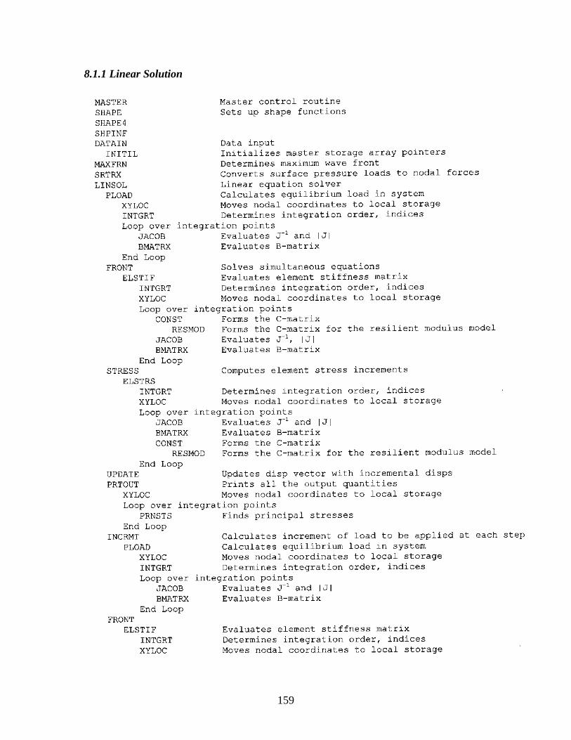
159

8.1.1 Linear Solution

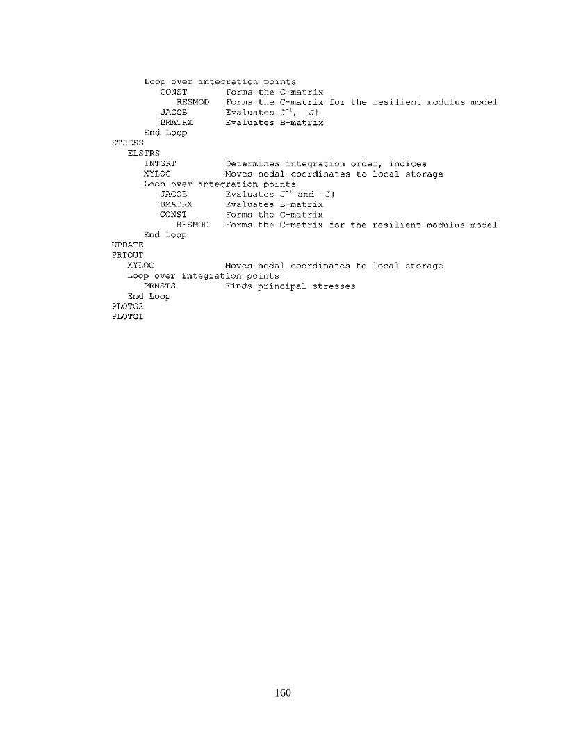
160

161

8.1.2 Nonlinear Solution

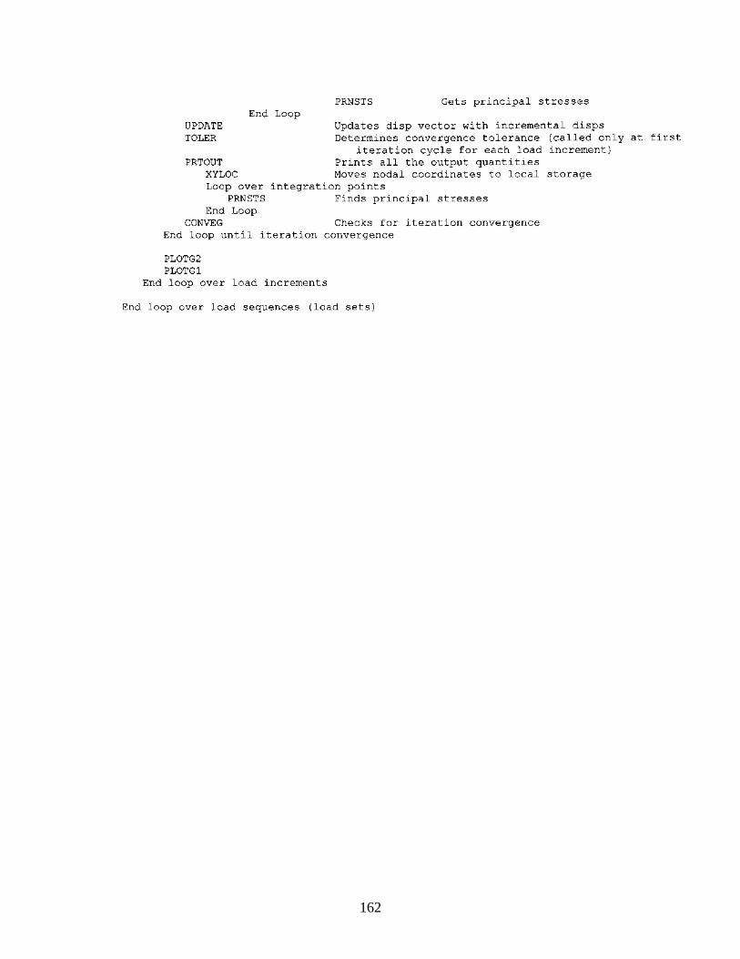
162

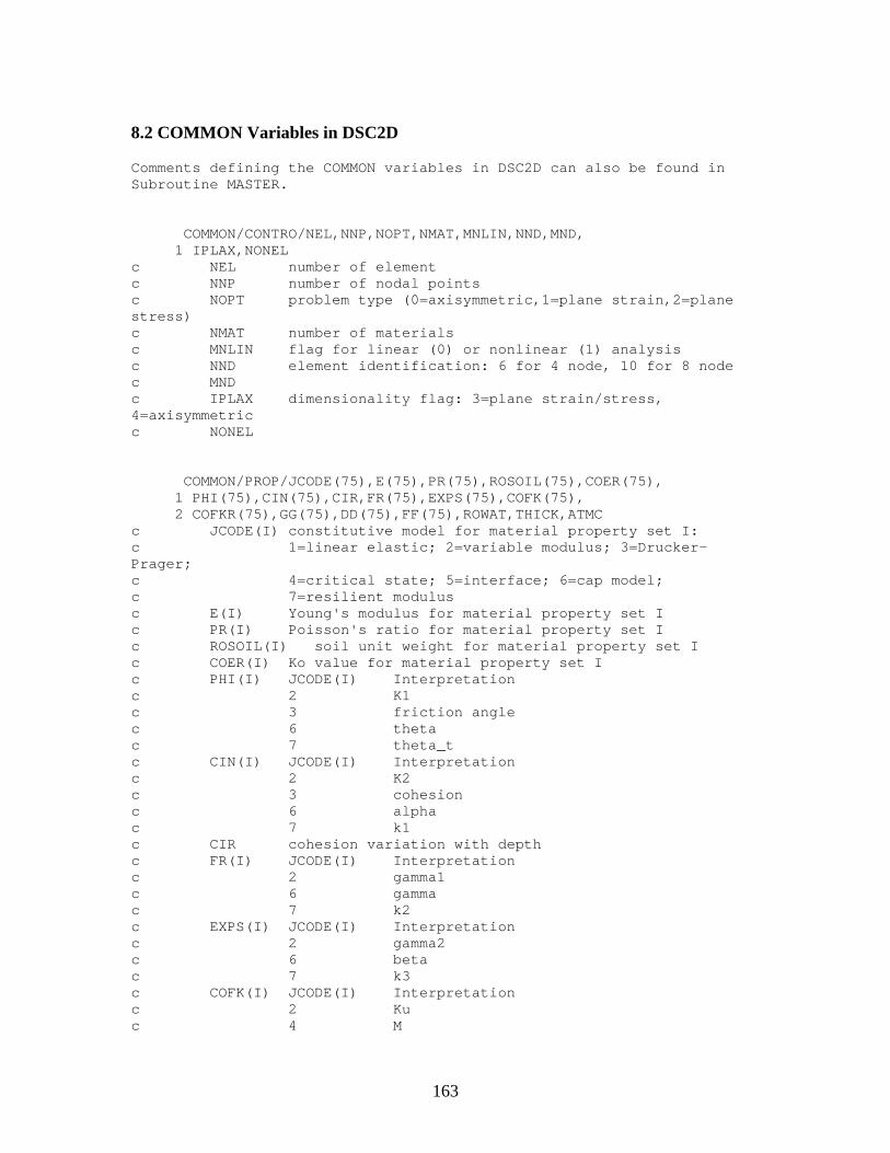
163

8.2 COMMON Variables in DSC2D

Comments defining the COMMON variables in DSC2D can also be found in Subroutine MASTER.

COMMON/CONTRO/NEL,NNP,NOPT,NMAT,MNLIN,NND,MND,

1 IPLAX,NONEL c NEL number of element c NNP number of nodal points c NOPT problem type (0=axisymmetric,1=plane strain,2=plane stress) c NMAT number of materials c MNLIN flag for linear (0) or nonlinear (1) analysis c NND element identification: 6 for 4 node, 10 for 8 node c MND c IPLAX dimensionality flag: 3=plane strain/stress, 4=axisymmetric c NONEL COMMON/PROP/JCODE(75),E(75),PR(75),ROSOIL(75),COER(75), 1 PHI(75),CIN(75),CIR,FR(75),EXPS(75),COFK(75), 2 COFKR(75),GG(75),DD(75),FF(75),ROWAT,THICK,ATMC c JCODE(I) constitutive model for material property set I: c 1=linear elastic; 2=variable modulus; 3=Drucker-Prager; c 4=critical state; 5=interface; 6=cap model; c 7=resilient modulus c E(I) Young's modulus for material property set I c PR(I) Poisson's ratio for material property set I c ROSOIL(I) soil unit weight for material property set I c COER(I) Ko value for material property set I c PHI(I) JCODE(I) Interpretation c 2 K1 c 3 friction angle c 6 theta c 7 theta_t c CIN(I) JCODE(I) Interpretation c 2 K2 c 3 cohesion c 6 alpha c 7 k1 c CIR cohesion variation with depth c FR(I) JCODE(I) Interpretation c 2 gamma1 c 6 gamma c 7 k2 c EXPS(I) JCODE(I) Interpretation c 2 gamma2 c 6 beta c 7 k3 c COFK(I) JCODE(I) Interpretation c 2 Ku c 4 M

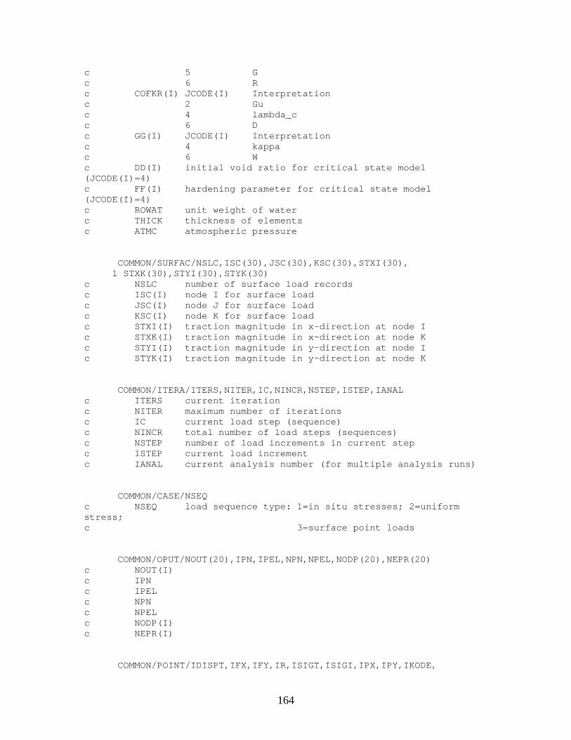
164

c 5 G c 6 R c COFKR(I) JCODE(I) Interpretation c 2 Gu c 4 lambda_c c 6 D c GG(I) JCODE(I) Interpretation c 4 kappa c 6 W c DD(I) initial void ratio for critical state model (JCODE(I)=4) c FF(I) hardening parameter for critical state model (JCODE(I)=4) c ROWAT unit weight of water c THICK thickness of elements c ATMC atmospheric pressure COMMON/SURFAC/NSLC,ISC(30),JSC(30),KSC(30),STXI(30), 1 STXK(30),STYI(30),STYK(30) c NSLC number of surface load records c ISC(I) node I for surface load c JSC(I) node J for surface load c KSC(I) node K for surface load c STXI(I) traction magnitude in x-direction at node I c STXK(I) traction magnitude in x-direction at node K c STYI(I) traction magnitude in y-direction at node I c STYK(I) traction magnitude in y-direction at node K COMMON/ITERA/ITERS,NITER,IC,NINCR,NSTEP,ISTEP,IANAL c ITERS current iteration c NITER maximum number of iterations c IC current load step (sequence) c NINCR total number of load steps (sequences) c NSTEP number of load increments in current step c ISTEP current load increment c IANAL current analysis number (for multiple analysis runs) COMMON/CASE/NSEQ c NSEQ load sequence type: 1=in situ stresses; 2=uniform stress; c 3=surface point loads COMMON/OPUT/NOUT(20),IPN,IPEL,NPN,NPEL,NODP(20),NEPR(20) c NOUT(I) c IPN c IPEL c NPN c NPEL c NODP(I) c NEPR(I) COMMON/POINT/IDISPT,IFX,IFY,IR,ISIGT,ISIGI,IPX,IPY,IKODE,

165

1 IUD,IUT,IX,IY,IKODEP,IFO,IGO,IFN,IEPSLT,IEPSLI,IFXTOT, 2 IFYTOT,IVOID,IP0,ICRIT,IIE,IFXT,IFYT c IDISPT pointer to beginning of system displacement vector c IFX pointer to beginning of system Fx vector c IFY pointer to beginning of system Fy vector c IR pointer to beginning of nodal displacement increments c (either for load increment or iteration cycl) c ISIGT pointer to beginning of element total stresses c A(ISIGT+36*M+4*IP-39) = sigma_x for element M c A(ISIGT+36*M+4*IP-38) = sigma_y for element M c A(ISIGT+36*M+4*IP-37) = tau_xy for element M c A(ISIGT+36*M+4*IP-36) = sigma_z for element M c ISIGI pointer to beginning of element stress increments c IPX pointer to beginning of initial u-displacement vector c IPY pointer to beginning of initial v-displacement vector c IKODE pointer to beginning of nodal boundary condition codes c IUD c IUT c IX pointer to beginning of system nodal x-coordinate vector c IY pointer to beginning of system nodal y-coordinate vector c IKODEP c IFO c IGO c IFN c IEPSLT pointer to beginning of element total strains c A(IEPSLT+36*M+4*IP-39) = epsilon_x for element M c A(IEPSLT+36*M+4*IP-38) = epsilon_y for element M c A(IEPSLT+36*M+4*IP-37) = gamma_xy for element M c A(IEPSLT+36*M+4*IP-36) = epsilon_z for element M c IEPSLI pointer to beginning of element strain increments c IFXTOT c IFYTOT c IVOID c IP0 c ICRIT c IIE pointer to beginning of system nodal connectivity array c For each element: c First NND-2 locations are the element nodal connectivity c NND-1 location is the element material type c NND location is the element integration order (0=2x2, 1=3x3) c IFXT c IFYT COMMON/FRONP/IIFFIX,IGSTIF,IEQUAT,IVECRV,IGLOAD,INACVA,MFRON 1 ,MSTIF,IIKOUN,IFIXED c IIFFIX c IGSTIF c IEQUAT pointer to beginning of equations for current wavefront c IVECRV c IGLOAD

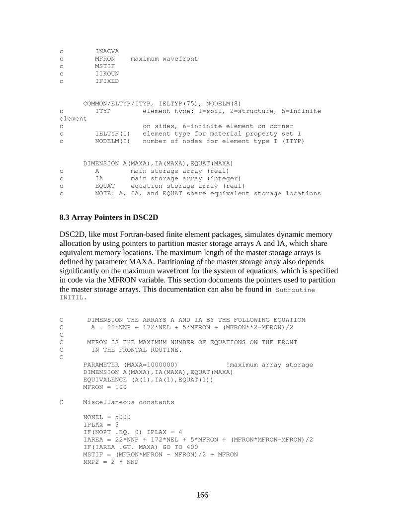
166

c INACVA c MFRON maximum wavefront c MSTIF c IIKOUN c IFIXED COMMON/ELTYP/ITYP, IELTYP(75), NODELM(8) c ITYP element type: 1=soil, 2=structure, 5=infinite element c on sides, 6=infinite element on corner c IELTYP(I) element type for material property set I c NODELM(I) number of nodes for element type I (ITYP) DIMENSION A(MAXA),IA(MAXA),EQUAT(MAXA) c A main storage array (real) c IA main storage array (integer) c EQUAT equation storage array (real) c NOTE: A, IA, and EQUAT share equivalent storage locations

8.3 Array Pointers in DSC2D

DSC2D, like most Fortran-based finite element packages, simulates dynamic memory allocation by using pointers to partition master storage arrays A and IA, which share equivalent memory locations. The maximum length of the master storage arrays is defined by parameter MAXA. Partitioning of the master storage array also depends significantly on the maximum wavefront for the system of equations, which is specified in code via the MFRON variable. This section documents the pointers used to partition the master storage arrays. This documentation can also be found in Subroutine INITIL. C DIMENSION THE ARRAYS A AND IA BY THE FOLLOWING EQUATION C A = 22*NNP + 172*NEL + 5*MFRON + (MFRON**2-MFRON)/2 C C MFRON IS THE MAXIMUM NUMBER OF EQUATIONS ON THE FRONT C IN THE FRONTAL ROUTINE. C PARAMETER (MAXA=1000000) !maximum array storage DIMENSION A(MAXA),IA(MAXA),EQUAT(MAXA) EQUIVALENCE (A(1),IA(1),EQUAT(1)) MFRON = 100 C Miscellaneous constants

NONEL = 5000

IPLAX = 3 IF(NOPT .EQ. 0) IPLAX = 4 IAREA = 22*NNP + 172*NEL + 5*MFRON + (MFRON*MFRON-MFRON)/2 IF(IAREA .GT. MAXA) GO TO 400 MSTIF = (MFRON*MFRON - MFRON)/2 + MFRON NNP2 = 2 * NNP

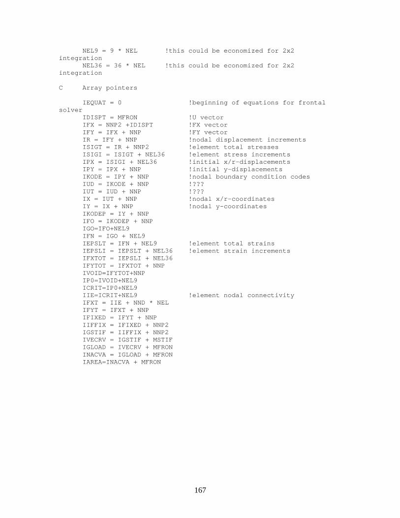
167

NEL9 = 9 * NEL !this could be economized for 2x2 integration NEL36 = 36 * NEL !this could be economized for 2x2 integration C Array pointers

IEQUAT = 0 !beginning of equations for frontal

solver IDISPT = MFRON !U vector IFX = NNP2 +IDISPT !FX vector IFY = IFX + NNP !FY vector IR = IFY + NNP !nodal displacement increments ISIGT = IR + NNP2 !element total stresses ISIGI = ISIGT + NEL36 !element stress increments IPX = ISIGI + NEL36 !initial x/r-displacements IPY = IPX + NNP !initial y-displacements IKODE = IPY + NNP !nodal boundary condition codes IUD = IKODE + NNP !??? IUT = IUD + NNP !??? IX = IUT + NNP !nodal x/r-coordinates IY = IX + NNP !nodal y-coordinates IKODEP = IY + NNP IFO = IKODEP + NNP IGO=IFO+NEL9 IFN = IGO + NEL9 IEPSLT = IFN + NEL9 !element total strains IEPSLI = IEPSLT + NEL36 !element strain increments IFXTOT = IEPSLI + NEL36 IFYTOT = IFXTOT + NNP IVOID=IFYTOT+NNP IP0=IVOID+NEL9 ICRIT=IP0+NEL9 IIE=ICRIT+NEL9 !element nodal connectivity IFXT = IIE + NND * NEL IFYT = IFXT + NNP IFIXED = IFYT + NNP IIFFIX = IFIXED + NNP2 IGSTIF = IIFFIX + NNP2 IVECRV = IGSTIF + MSTIF IGLOAD = IVECRV + MFRON INACVA = IGLOAD + MFRON IAREA=INACVA + MFRON

168

9. REFERENCES

Ahlborn, G. (1972) Elastic Layered System with Normal Loads, The Institution of Transportation and Traffic Engineering, University of California—Berkeley. Ahlvin, R.G., et al. (1971) “Multiple-Wheel Heavy Gear Load Pavement Tests,” Technical Report S-71-17, Vol. I-IV, U.S. Army Waterways Experiment Station, Vicksburg, MS, November. Andrei, D. (2001) personal communication. Andrei, D. (1999) Development of a Harmonized Test Protocol for the Resilient Modulus of Unbound Materials Used in Pavement Design, M.S. Thesis, University of Maryland—College Park. Asphalt Institute (1991) DAMA (CP-1/1991 Revision)—Pavement Structural Analysis Using Muli-Layered Elastic Theory, Lexington, KY. Ayres, M. (1997) Development of a Rational Probabilistic Approach for Flexible Pavement Analysis, Ph.D. Dissertation, University of Maryland, College Park, MD. Barker, W., and Gonzalez, C. (1991) “Pavement Design by Elastic Layer Theory, Proceedings, Conference on Aircraft/Pavement Interaction—An Integrated System, ASCE. Bathe, K.J. (1996) Finite Element Procedures, Prentice-Hall, Englewood Cliffs, NJ. Beer, C., and Meek, J.L. (1981) “Infinite Domain Elements,” International Journal for Numerical Methods in Engineering, Vol. 17, pp. 43-52. Bettess, P. (1977) “Infinite Elements,” International Journal for Numerical Methods in Engineering, Vol. 11, pp. 53-64. Bettess, P., and Zienkiewicz, O.C. (1977) “Diffraction and Refraction of Surface Waves Using Finite and Infinite Elements,” International Journal for Numerical Methods in Engineering, Vol. 11, pp. 1271-90. Brill, D.R., Hayhoe, G.F., and Lee, X. (1997) “Three Dimensional Finite Element Modeling of Rigid pavement Structures,” Aircraft/Pavement Technology: In the Midst of Change (F.V. Hermann, ed.), Proceedings, ASCE Airfield Pavement Conference, Seattle, WA, pp. 151-165. Brown, S.F., and Pappin, J.W. (1981) “Analysis of Pavements with Granular Bases,” Transportation Research Record, Transportation Research Board, National Research Council, Washington, DC, pp. 17-23.

169

Burmister, D.M. (1943) “The Theory of Stresses and Displacements In Layered Systems and Applications to the Design of Airport Runways,” Proceedings, Highway Research Board, Vol. 23. Chen, D.H., Zaman, M., Laguros, J., and Soltani, A. (1995) “Assessment of Computer Programs for Analysis of Flexible Pavement Structures,” Transportation Research Record 1539, Transportation Research Board, National Research Council, Washington, DC, pp. 123-133. Cho, Y.-H., McCullough, B.F., and Weissmann, J. (1996) “Considerations on Finite-Element Method Application in Pavement Structural Analysis,” Transportation Research Record 1539, TRB, National Research Council, Washington, DC, pp. 96-101. Chou, Y.T., and Ledbetter, R.H. (1973) “The Behavior of Flexible Airfield Pavements Under Loads—Theory and Experiments,” Report M.P. S-73-66, U.S. Army Engineer Waterways Experiment Station, Vicksburg, MS, July. Computer Program DAMA—Pavement Structural Analysis Using Multi-Layered Elastic Theory, Report CP-1 (1991 Revision), The Asphalt Institute, Lexington, KY.

Dai. S.T., Van Deusen, D., Beer, M., Rettner, D., and Cochran, G. (1997) “Investigation of Flexible Pavement Response to Truck Speed and FWD Load Through Instrumented Pavements,” Proceedings, Eighth International Conference on Asphalt Pavements, Seattle, Washington, Vol. 1, pp. 141-160. Davids, W. (1998) “EverFE: A Rigid Pavement 3D Analysis Tool,” 1998 Annual Meeting of the Transportation Research Board, Washington, DC, January. Desai, C.S. (2000) User’s Manual for the DSC-2D Code for the 2002 Design Guide (in preparation). Desai, C.S., and Abel, J.F. (1972) Introduction to the Finite Element Method, Van Nostrand Reinhold, New York. Desai, C.S., and Schwartz, C.W. (2000) Selection of Finite Element Program for Flexible Pavement Response Model, unpublished NCHRP Project 1-37A working paper, January. Desai, C.S., and Siriwardane. H.J. (1984) Constitutive Laws For Engineering Materials, With Emphasis On Geologic Materials, Prentice-Hall, Inc., Englewood Cliffs, NJ. Duncan, J.M, Monismith, C.L., and Wilson, E.L. (1968) “Finite Element Analysis of Pavements,” Highway Research Record #228, Transportation Research Board, Washington, DC.

170

Ertman Larsen, H.J., and Ullidtz, P. (1997) “Pavement Subgrade Performance Study in the Danish Road Testing Machine,” Proceedings, Eighth International Conference on Asphalt Pavements, Seattle, Washington, Vol. 1, pp. 843-857. GAO (1997) “Transportation Infrastructure: Highway Pavement Design Guide is Outdated,” United States General Accounting Office, Gaithersburg, MD, November. Hammons, M. (1998) “Validation of Three-Dimensional Finite Element Modeling Technique for Jointed Concrete Pavements,” 1998 Annual Meeting of the Transportation Research Board, Washington, DC, January. Harichandran, R.W., Yeh, M.-S., and Baladi, G.Y. (1989) MICH-PAVE User’s Manual, Final Report, FHWA-MI-RD-89-023, Department of Civil and Environmental Engineering, Michigan State University , East Lansing, MI. Harichandran, R.S., Yeh, M.-S., and Baladi, G.Y. (1990) “MICH-PAVE: A Nonlinear Finite Element Program for the Analysis of Flexible Pavements,” Transportation Research Record, No. 1286. Hermann, F.V. (ed., 1997). Aircraft Pavement Technology: In the Midst of Change, Proceedings, ASCE Airfield Pavement Conference, Seattle, WA. Hibbitt, Karlsson, and Sorensen (1998) ABAQUS/Standard User’s Manual (Version 5.8), Hibbitt, Karlsson, and Sorensen, Inc., Pawtucket, RI. Hjelmsted, K.D., Kim, J., and Zuo, Q. (1997) “Finite Element Procedures for Three Dimensional Pavement Analysis,” Aircraft/Pavement Technology: In the Midst of Change (F.V. Hermann, ed.), Proceedings, ASCE Airfield Pavement Conference, Seattle, WA, pp. 125-137. Hjelmstad, K.D., and Taciroglu, E. (2000) “Analysis and Implementation of Resilient Modulus Models for Granular Soils,” Journal of Engineering Mechanics, ASCE (in press). Huang, Y.H. (1993) Pavement Analysis and Design, Prentice-Hall, Inc., Englewood Cliffs, NY. ILLI-PAVE PC Version User’s Manual (1990), NCHRP Project 1-26, Transportation Facilities Group, University of Illinois, Urbana-Champaign, IL. Livermore Software Technology Corporation (1999) LS-DYNA Keyword User’s Manual (Version 950), Livermore Software Technology Corporation, Livermore, CA. Lytton, R.L., Uzan, J., Fernando, E.G., Roque, R., Hiltunen, D. Stoffels, S.M. (1993) “Development and Validation of Performance Prediction Models and Specifications for

171

Asphalt Binders and Paving Mixes,” Report SHRP A-357, Strategic Highway Research Program, National Research Council, Washington, DC. Michelow, J. (1963) Analysis of Stresses and Displacements in an N-Layered Elastic System Under a Load Uniformly Distributed on a Circular Area, California Research Corporation, Richmond, CA. Poulos, H.G., and Davis, E.H. (1974) Elastic Solutions for Soil and Rock Mechanics, John Wiley and Sons, Inc., New York, NY. Raad, L., and Figueroa, J.L. (1980) “Load Response of Transportation Support Systems,” Transportation Engineering Journal, ASCE, Vol. 106, No. TE1. Schwartz, C.W. (2000) “Effect of Stress-Dependent Base Layer on the Superposition of Two-Dimensional Flexible Pavement Solutions,” Proceedings, 2nd International Conference on 3D Finite Elements for Pavement Analysis, Design, and Research, Charleston, WV, October, pp. 329-354. Schwartz, C.W. (2001) “Implementation of a Nonlinear Resilient Modulus Constitutive Model for Unbound Pavement Materials,” Proceedings, 10th International Conference on Computer Methods and Advances in Geomechanics, Tucson, AZ, January, pp. 1385-1390. Shell Oil Co. (1978) BISAR: Bitumen Structures Analysis in Roads User’s Manual, Boninklijke/Shell Laboratorium, Shell Research N.V., Amsterdam, The Netherlands. Shoukry, S. (1998a) “3D Finite Element Modeling for Pavement Analysis and Design,” Finite Element for Pavement Analysis and Design, (S. Shoukry, ed.), Proceedings, First National Symposium on 3D Finite Element Modeling for Pavement Analysis and Design, Charleston, WV, November, pp. 1-51. Shoukry, S. (ed., 1998b). Finite Element for Pavement Analysis and Design, Proceedings, First National Symposium on 3D Finite Element Modeling for Pavement Analysis and Design, Charleston, WV, November. Texas Transportation Institute (1991) SHRP Quarterly Report for Contract A-005: Performance Models and Validation of Test Results, Quarter 2 of 4 of Year 2, July. Thompson, M.R. (1990) “NCHRP 1-26: Calibrated Mechanistic Structural Analysis Procedures for Pavements. Volume I - Final Report,” prepared for the National Cooperative Highway Research Program, Transportation Research Board, National Research Council, Washington, DC, March. Thompson, M.R., and Garg, N. (1999) “Wheel Load Interaction: Critical Airport Pavement Responses,” COE Report No. 7, Center of Excellence for Airport Pavement

172

Research, Department of Civil Engineering, University of Illinois at Urbana-Champaign, July. Tutumluer, E. (1995) Predicting Behavior of Flexible Pavements with Granular Bases, Ph.D. Dissertation, School of Civil and Environmental Engineering, Georgia Institute of Technology, Atlanta, GA. Uddin, W. (1998) “Application of 3D Finite Element Dynamic Analysis for Pavement Evaluation,” Finite Element for Pavement Analysis and Design, (S. Shoukry, ed.), Proceedings, First National Symposium on 3D Finite Element Modeling for Pavement Analysis and Design, Charleston, WV, November, pp. 94-110. Ullidtz, P. (1998) Modelling Flexible Pavement Response and Performance, Polyteknisk Forlag, Denmark. Ullidtz, P., Askegaard, V., and Sjolin, F.O. (1996) “Normal Stresses in a Granular Material Under Falling Weight Deflectometer Loading,” Transportation Research Record 1540, Transportation Research Board, National Research Council, Washington, DC, pp 24-28. Ullidtz, P., and Peattie, K.R. (1980) “Pavement Analysis by Programmable Calculators,” Transportation Engineering Journal, ASCE, Vol. 106, No. TE5. U.S. Army Engineer Waterways Experiment Station (1951) “Investigations of Pressures and Deflections for Flexible Pavements: Report 1, Homogeneous Clayey-Silt Test Section,"”Technical Memorandum No. 3-323, Vicksburg, MS, March. U.S. Army Engineer Waterways Experiment Station (1954) “Investigations of Pressures and Deflections for Flexible Pavements: Report 4, Homogeneous Sand Test Section,"”Technical Memorandum No. 3-323, Vicksburg, MS, December. Uzan, J. (1985) “Characterization of Granular Material,” Transportation Research Record 1022, TRB, National Research Council, Washington, DC, pp. 52-59. Uzan, J. (1991) “SHRP Quarterly Report: A-005 Performance Models and Validation of Test Results. Quarter 2 of 4, of Year 2,” Texas Transportation Institute, The Texas A&M University System, College Station, Texas, July 15. Van Cauwelaert, F.J., Barker, W.J., White, T.D., and Alexander, D.R. (1988) “A Competent Multilayer Solution and Backcalculation Procedure for Personal Computers,” Special Technical Publication 1026, ASTM, Washington, DC. White, T. (1998) “Application of Finite Element Analysis to Pavement Problems,” Finite Element for Pavement Analysis and Design, (S. Shoukry, ed.), Proceedings, First National Symposium on 3D Finite Element Modeling for Pavement Analysis and Design, Charleston, WV, November, pp. 52-84.

173

Witczak, M.W., and Uzan, J. (1988) The Universal Airport Pavement Design System. Report I of V: Granular Material Characterization, Department of Civil Engineering, University of Maryland, College Park, MD. Yoder, E.J., and Witczak, M.W. (1975) Principles of Pavement Design (2nd Edition), John Wiley and Sons, Inc., New York, NY. Zaghoul, S., and White, T. (1993) “Use of a Three-Dimensional Dynamic Finite Element Program for Analysis of Flexible Pavements,” Transportation Research Record 1388, Transportation Research Board, National Research Council, Washington, DC, pp 60-69. Zienkiewicz, O.C. (1977) The Finite Element Method (Third Edition), McGraw-Hill, New York. Zienkiewicz, O.C., Emson, C., and Bettess, P. (1983) “A Novel Boundary Infinite Element,” International Journal for Numerical Methods in Engineering, Vol. 19, pp. 393-404. Zienkiewicz, O.C., and Taylor, R.L. (1989) The Finite Element Method (Fourth Edition), McGraw-Hill, New York.

174

10. ALTERNATIVE FORMULATION FOR NONLINEAR MR

The derivations here follow the general approach employed by Uzan in the SHRP performance prediction models (Lytton et al., 1993). From Figure 30, and taking the axial direction equal to the x-direction:

( )1x xo x xo x

RMε ε ε ε σ= + ∆ = + ∆ (49)

in which εxo is the initial axial strain induced by the initial confining pressure σxo, ∆εx is the resilient axial strain, and x x xoσ σ σ∆ = − is the cyclic axial stress. Generalizing Eq. (49) to multidimensional stress conditions:

( )1x xo x y z

RMε ε σ ν σ σ⎡ ⎤= + ∆ − ∆ + ∆⎣ ⎦ (50)

in which y y yoσ σ σ∆ = − , z z zoσ σ σ∆ = − , σyo and σzo are the initial lateral confining pressures, and ν = Poisson’s ratio, which is assumed to be stress-independent. Using the standard assumption σyo = σzo = Koσxo with σxo now interpreted as the initial vertical overburden stress, Eq. (50) can be written alternatively as:

( ) ( )1 1 2x xo x y z o xoR

KM

ε ε σ ν σ σ ν σ⎡ ⎤= + − + − −⎣ ⎦ (51)

The x-direction strain can be expressed in incremental form as:

x x x x x xx x y z xy yz zx

x y z xy yz zx

ε ε ε ε ε εε σ σ σ τ τ τσ σ σ τ τ τ

∂ ∂ ∂ ∂ ∂ ∂= + + + + +

∂ ∂ ∂ ∂ ∂ ∂& & & & & & & (52)

in which , , i j ijε σ τ& & & are the strain and stress increments. Eq. (51) can be generalized to the other strain components and used to derive the terms of the incremental (or tangent) compliance matrix tD

%:

tDε σ=& &

%% % (53)

in which , ε σ& &

% % are the incremental strain and stress vectors. The incremental (tangent)

material stiffness matrix tC%

can be determined from the inverse of tD%

: 1

t tC Dσ ε ε−= =& &&%% % % %

(54) Note that tC

% will not in general be symmetric.

175

Under certain stress conditions, the bottom of an unbound layer may approach a tensile stress condition, i.e., θ → 0. Then MR as defined by Eq. (8) will also go to zero. This can be treated in the finite element implementation by assigning an arbitrarily small value to the tangent modulus ET for these conditions. The above formulation was implemented into the ABAQUS finite element code and tested for accuracy. Figure 86 and Figure 87 show comparisons for two different sets of material parameters between single-element finite element calculations and the analytical solution of Eq. (8) for the case of a monotonic triaxial compression loading. The finite element calculations agree well with the analytical values. The degree of agreement increases as the number of load steps increases (load step size decreases), as expected. The simpler nonlinear MR formulation described previously in Section 4.2 and the alternative formulation summarized in this section give identical predictions for standard triaxial loading paths--i.e., constant confining pressure and monotonically increasing deviator stress. The two formulations give different predictions for other more general load paths. Unfortunately, however, little resilient modulus test data exist in the literature for nonstandard load paths and thus it is impossible to evaluate which formulation is more realistic. This shortcoming, plus the complications associated with the lack of symmetry for tC

% in Eq. (54), were the principal reasons that the more generally accepted

and simpler nonlinear MR formulation described in Section 4.2 was implemented in the DSC2D finite element program for the 2002 Design Guide.

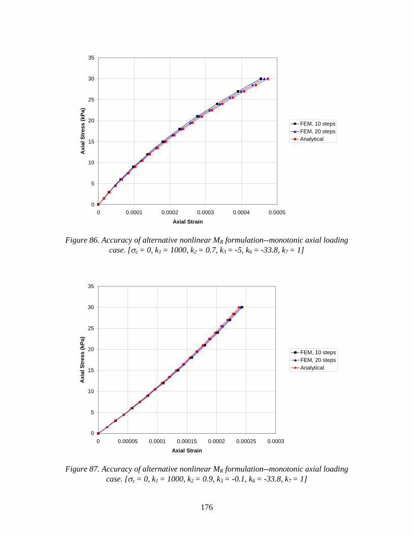
176

0

5

10

15

20

25

30

35

0 0.0001 0.0002 0.0003 0.0004 0.0005

Axial Strain

Axi

al S

tres

s (k

Pa)

FEM, 10 stepsFEM, 20 stepsAnalytical

Figure 86. Accuracy of alternative nonlinear MR formulation--monotonic axial loading

case. [σc = 0, k1 = 1000, k2 = 0.7, k3 = -5, k6 = -33.8, k7 = 1]

0

5

10

15

20

25

30

35

0 0.00005 0.0001 0.00015 0.0002 0.00025 0.0003

Axial Strain

Axi

al S

tres

s (k

Pa)

FEM, 10 stepsFEM, 20 stepsAnalytical

Figure 87. Accuracy of alternative nonlinear MR formulation--monotonic axial loading

case. [σc = 0, k1 = 1000, k2 = 0.9, k3 = -0.1, k6 = -33.8, k7 = 1]

177

Annex B Comparison of Layered Elastic Analysis Program (APADS) with the Finite Element

Analysis Used in the 2002 Design Guide

178

FORWARD

The work reported herein has been conducted as a part of project “Development of the 2002

Guide for the Design of New and Rehabilitated Pavement Structures” under the contract with

National Cooperative Highway Research Program, NCHRP 1-37A. Dr. M. W. Mirza

authored the report under the technical direction and supervision of Dr. M. W. Witczak,

Project Principal Investigator and Professor at Arizona State University. Dr. Charles

Schwartz of University of Maryland, who was responsible for the development of the finite

element module, Dr. Manuel Ayres who was mainly responsible for the integration of the

layered elastic solution in the 2002 Deign Guide and finally, Dr. Jacob Uzan who is the

developer of JULEA (Layered Elastic Program) provided valuable comments and their help is

greatly acknowledged.

In the 2002 Design Guide the two major modules are the APADS (layered elastic

solution) and the finite element module (FEM). The finite element module can be used

both for the linear and non-linear analysis. That is, both the APADS and FEM can be

used for pavement response, if all the pavement layers in the pavement system are

defined as linear elastic. It is important that in situation if all the layers are characterized

as linear, both analyses generate comparable results.

The objective of this report was to compare the results from APADS and the FEM. It was

found that the response from both the analysis were very similar. A small difference in the

results was due to the different mathematical approach and approximations used in finite

element analysis. However, for all practical purposed the results were considered acceptable

for the determination of distresses from either of the analysis module.

179

TABLE OF CONTENTS

FORWARD ………………………………………………………………………….. ii

TABLE OF CONTENTS ……………………………………………………………… iii

LIST OF FIGURES ……………………………………………………………………. iv

BACKGROUND ………………………………………………………………………. 1

RESPONSE TO DISTRESS RELATIONSHIP ……………………………………….. 3

NON-LINEAR CHARACTERIZATION IN 2002 DESIGN GUIDE ………………… 4

FINITE ELEMENT ANALYSIS ……………………………………………………… 6

Linearity Check with FEA …………………………………………………….. 6

Independence…………………………………………………………………… 8

General and Special Traffic Analysis ………………………………………….. 9

COMPARISON OF LEA AND FEA ………………………………………………….. 12

Conventional Pavement Structure with General Traffic ………………………. 12

Effect of Axle Configuration…………………………………………………… 16

Special Gear Configuration ……………………………………………………. 19

SUMMARY ……………………………………………………………………………. 23

180

LIST OF FIGURES

Figure No. Page

1. Verification of Linearity with Tensile Strain Response at the Bottom of

Asphalt Layer for a Three Layer Pavement Structure ………………………. 7

2. Verification of Linearity with Bulk Stress Response in an Unbound Layer

for a Three layer Pavement Structure………………………………………… 7

3. Verification of Independence with Tensile Strain Response at the Bottom

of Asphalt Layer……………………………………………………………… 10

4. Verification of Independence with Bulk Stress Response within the

Unbound Layer ………………………………………………………………. 10

5a. Tensile Strain Comparison Between General and Special Traffic…………… 11

5b. Comparison Between General and Special Traffic (Vertical Strain,

Deviator and Bulk Stress) …………………………………………………… 11

6. Schematic of Original Pavement Structure and the Sub-Layering ………….. 13

7a. Comparison of FEM and LEA for the Tensile Strain at Three Depths………. 15

7b. Percent Difference Between FEA and the LEA at Three Depths ……………. 15

8a. Comparisons of Strains and Stresses at the Mid-Depth of Fourth Sub Layer.. 17

8b. Stress and Strain Difference at the Mid-Depth of Fourth Sub-Layer………… 17

9a. Comparisons of Strains and Stresses Six Inches Below the Semi-Infinite

Layer ………………………………………………………………………… 18

9b. Stress and Strain Difference Six Inches Below the Semi-Infinite Layer …….. 18

10a. Comparisons of Tensile Strains as a Function of Axle Configuration ………. 20

10b. Tensile Strain Difference as a Function of Axle Configuration …………….. 20

11a. Comparisons of Bulk Stress as a Function of Axle Configuration…………… 21

11b. Bulk Stress Difference as a Function of Axle Configuration ……………….. 21

12. Special Gear Configurations for FEA and LEA Comparison ……………….. 22

13a. Special Gear Comparisons of Tensile Strain at Three Depths ……………… 24

13b. Tensile Strain Difference with Depth ………………………………………. 24

181

LIST OF FIGURES (Cont’d)

Figure No. Page

14a. Comparisons of Strains and Stresses in Unbound Granular Layer for

Special Gear Configurations …………………………………………………. 25

14b. Difference in Strains and Stresses in Unbound Granular Layer for

Special Gear Configurations …………………………………………………. 25

182

COMPARISON OF LAYERED ELASTIC ANALYSIS PROGRAM

(APADS) WITH FINITE ELEMENT ANALYSIS USED IN

THE 2002 DESIGN GUIDE

BACKGROUND

Accurate pavement performance prediction is widely recognized by pavement

community as one of the most important, complex and difficult task to pursue. The

important of such a goal cannot be overemphasized because this will result in the saving

of millions of dollars. Proper selection of pavement materials and layer thickness can be

optimized based upon performance-based specification. The basic requirement for this is

the availability of the accurate pavement performance prediction methodology.

Historically, the analysis of pavement systems dates back to the late 1920’s when

empirical

design methods were first introduced. The major advantage of these methods is the

mathematical simplicity that does not require advanced computational capabilities or

extensive material characterization for the design of pavement structures. However with

all these advantages, the empirical methods are with some serious limitations. The major

limitation of such empirical techniques is that they cannot provide accurate prediction for

material, environment and traffic conditions that differ from those for which the models

were originally developed. It was not until sixties that mechanistic-empirical procedures

started to be implemented for the pavement analysis and design. These techniques

introduced, uses pavement response in terms of stresses and strains as major causative

factors affecting pavement performance. It is well understood that the pavement

response, such as the stresses and strains in the system are directly related to the

pavement layer material properties. Thus, characterization of these materials is an

important factor in the measurement of the response. In general the layer materials can

183

be characterized as linear elastic, non-linear elastic or linear visco-elastic depending upon

the material type and accuracy desired.

Interaction among pavement layers (material properties and thickness), environmental

condition, applied load and variability of these factors will dictate when and where

distress will initiate as well as the rate these distresses will progress. The development of

the distress within the pavement system is a function of the critical stresses and strains

that are developed within the pavement system as a result of traffic loading and

environmental effects. With the current state of knowledge the estimation of the stresses

and strains can be estimated by theory of elasticity for linear analysis and is usually

termed as the Layered Elastic Analysis (LEA). This analysis may or may not be accurate

since in the actual situation most of the paving materials especially the unbound material

behaves non-linearly under load and thus cannot be properly characterize by linear

analysis. Several techniques have been used in the past to characterize non-linear nature

of the unbound material, however the most common among these techniques is the Finite

Element Analysis (FEA).

The Layered Elastic Analysis (LEA) is based upon the theory of elasticity. This method

uses fundamental physical properties and a theoretical model to predict the stresses,

strains and deflections, i.e. the pavement response, caused by a load on the pavement. If

the basic assumptions with respect to materials and boundary conditions are correct, this

method is valid anywhere and may used to correctly predict the response for any

combination of loads, climatic effects and materials.

At present several computer programs are available to determine the pavement response

using the layered elastic analysis. Some of the more well known are the programs

developed by Shell (Bistro and Bisar), by Chevron (Elsym5), Water-ways Experiment

Station (WES5), the Laboratoire Central des Ponts et Chaussees (Alize III), the

Commonwealth Scientific and Industrial Research Organization (Circly) and the Jacob

Uzan Layered Elastic Analysis (JULEA).

184

All the above-mentioned programs are based on linear elastic theory and assume all layer

materials to be linear. As mentioned earlier, some pavement materials especially the

unbound materials show non-linear behavior under load and are usually termed as non-

linear elastic. No analytical solution presently exists for the non-linear stress-strain

relationship, but with Finite Element Analysis (FEA), it is possible to treat non-linear

elastic materials, through an iterative process. Because of the complex mathematical

computational nature of the analysis, limited number of finite element programs has been

developed in the past for characterizing the non-linear behavior of pavement layers. But

with the advent of the fast computers and reduced processing times, finite element

analysis is becoming more popular.

In the case of 2002 Design Guide for the design of pavement structures both linear and

non-linear behavior characterization of pavement layers is possible. That is, the

pavement response under the traffic loading can be determined by treating the material as

linear or non-linear. It is important to recognize that within the 2002 Design Guide,

unbound granular material can only be defined as linear or non-linear. All bituminous

and stabilized layers are always treated as linear and the option is not available to

characterize the behavior of these materials as being non-linear. This was done, since

these materials only shows non-linear behavior under very extreme conditions and under

most field situations their behavior is close to linear. Thus, characterizing these layer

materials as linear will not introduce any significant error in the analysis. In addition, at

present no acceptable models are available to characterize bituminous and cement treated

material as non-linear under these extreme conditions.

RESPONSE TO DISTRESS RELATIONSHIP

The pavement response obtained from these response models are used for the estimation

of pavement distress. The distress is then used for the pavement performance evaluation.

The distresses include computation of fatigue, permanent deformation and thermal

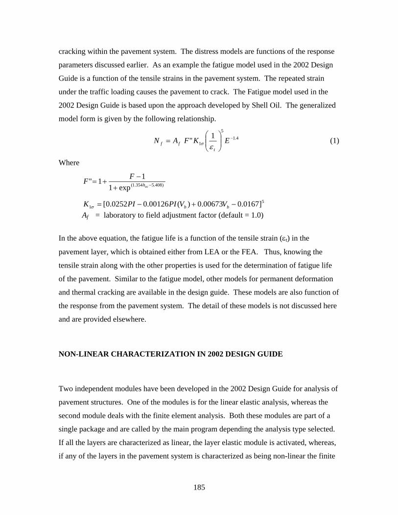
185

cracking within the pavement system. The distress models are functions of the response

parameters discussed earlier. As an example the fatigue model used in the 2002 Design

Guide is a function of the tensile strains in the pavement system. The repeated strain

under the traffic loading causes the pavement to crack. The Fatigue model used in the

2002 Design Guide is based upon the approach developed by Shell Oil. The generalized

model form is given by the following relationship.

4.15

11" −

⎟⎟⎠

⎞⎜⎜⎝

⎛= EKFAN

tff εσ (1)

Where

)408.5354.1(exp111" −+

−+=

ach

FF

51 ]0167.000673.0)(00126.00252.0[ −+−= bb VVPIPIK σ

Af = laboratory to field adjustment factor (default = 1.0)

In the above equation, the fatigue life is a function of the tensile strain (εt) in the

pavement layer, which is obtained either from LEA or the FEA. Thus, knowing the

tensile strain along with the other properties is used for the determination of fatigue life

of the pavement. Similar to the fatigue model, other models for permanent deformation

and thermal cracking are available in the design guide. These models are also function of

the response from the pavement system. The detail of these models is not discussed here

and are provided elsewhere.

NON-LINEAR CHARACTERIZATION IN 2002 DESIGN GUIDE

Two independent modules have been developed in the 2002 Design Guide for analysis of

pavement structures. One of the modules is for the linear elastic analysis, whereas the

second module deals with the finite element analysis. Both these modules are part of a

single package and are called by the main program depending the analysis type selected.

If all the layers are characterized as linear, the layer elastic module is activated, whereas,

if any of the layers in the pavement system is characterized as being non-linear the finite

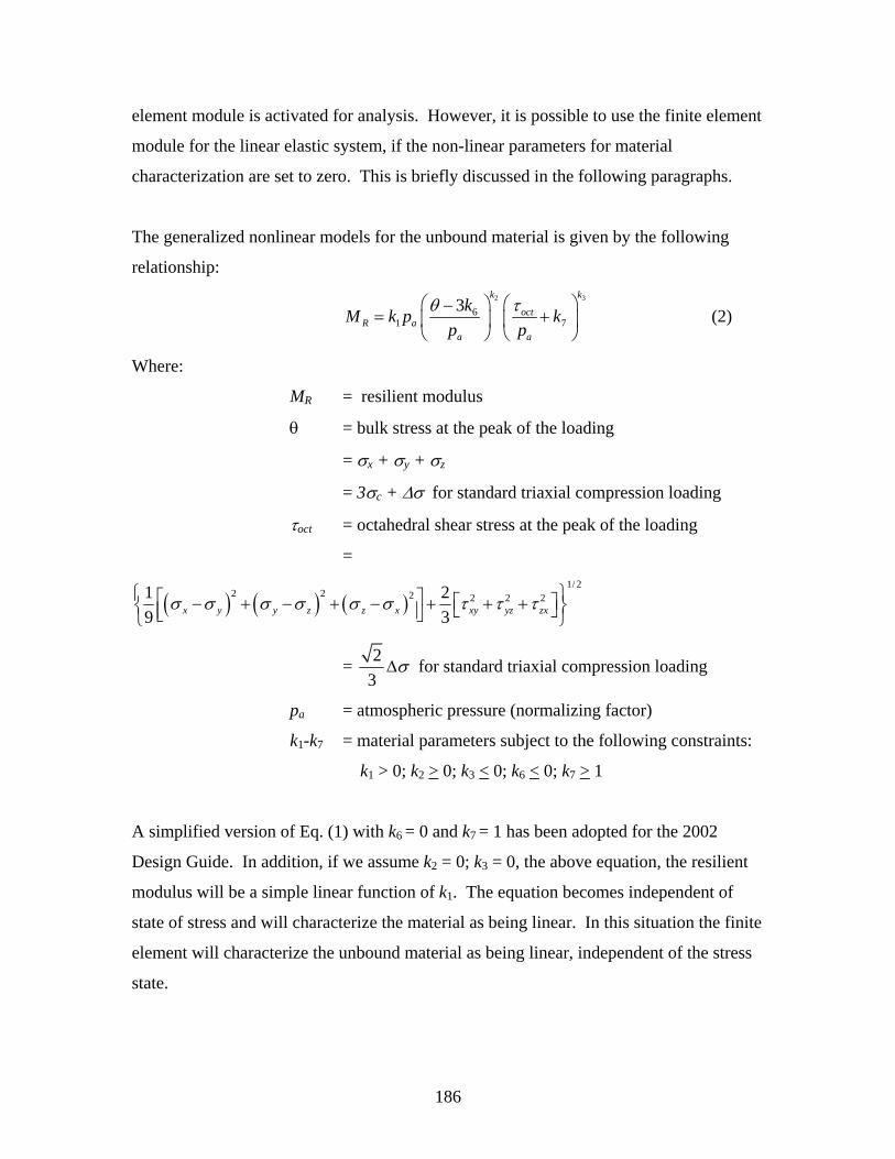
186

element module is activated for analysis. However, it is possible to use the finite element

module for the linear elastic system, if the non-linear parameters for material

characterization are set to zero. This is briefly discussed in the following paragraphs.

The generalized nonlinear models for the unbound material is given by the following

relationship: 2 3

61 7

3k k

octR a

a a

kM k p kp p

θ τ⎛ ⎞ ⎛ ⎞−= +⎜ ⎟ ⎜ ⎟

⎝ ⎠ ⎝ ⎠ (2)

Where:

MR = resilient modulus

θ = bulk stress at the peak of the loading

= σx + σy + σz

= 3σc + ∆σ for standard triaxial compression loading

τoct = octahedral shear stress at the peak of the loading

=

( ) ( ) ( )1/ 2

2 2 2 2 2 21 29 3x y y z z x xy yz zxσ σ σ σ σ σ τ τ τ⎧ ⎫⎡ ⎤ ⎡ ⎤− + − + − + + +⎨ ⎬⎣ ⎦⎢ ⎥⎣ ⎦⎩ ⎭

= 23

σ∆ for standard triaxial compression loading

pa = atmospheric pressure (normalizing factor)

k1-k7 = material parameters subject to the following constraints:

k1 > 0; k2 > 0; k3 < 0; k6 < 0; k7 > 1

A simplified version of Eq. (1) with k6 = 0 and k7 = 1 has been adopted for the 2002

Design Guide. In addition, if we assume k2 = 0; k3 = 0, the above equation, the resilient

modulus will be a simple linear function of k1. The equation becomes independent of

state of stress and will characterize the material as being linear. In this situation the finite

element will characterize the unbound material as being linear, independent of the stress

state.

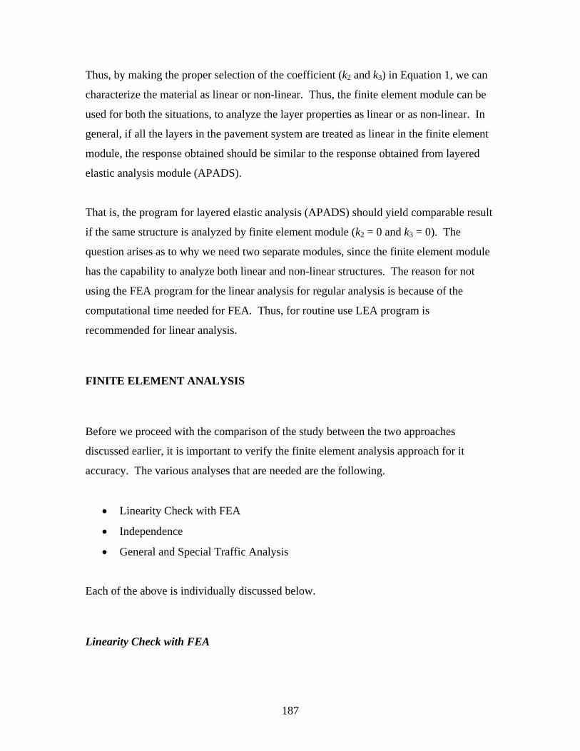
187

Thus, by making the proper selection of the coefficient (k2 and k3) in Equation 1, we can

characterize the material as linear or non-linear. Thus, the finite element module can be

used for both the situations, to analyze the layer properties as linear or as non-linear. In

general, if all the layers in the pavement system are treated as linear in the finite element

module, the response obtained should be similar to the response obtained from layered

elastic analysis module (APADS).

That is, the program for layered elastic analysis (APADS) should yield comparable result

if the same structure is analyzed by finite element module (k2 = 0 and k3 = 0). The

question arises as to why we need two separate modules, since the finite element module

has the capability to analyze both linear and non-linear structures. The reason for not

using the FEA program for the linear analysis for regular analysis is because of the

computational time needed for FEA. Thus, for routine use LEA program is

recommended for linear analysis.

FINITE ELEMENT ANALYSIS

Before we proceed with the comparison of the study between the two approaches

discussed earlier, it is important to verify the finite element analysis approach for it

accuracy. The various analyses that are needed are the following.

• Linearity Check with FEA

• Independence

• General and Special Traffic Analysis

Each of the above is individually discussed below.

Linearity Check with FEA

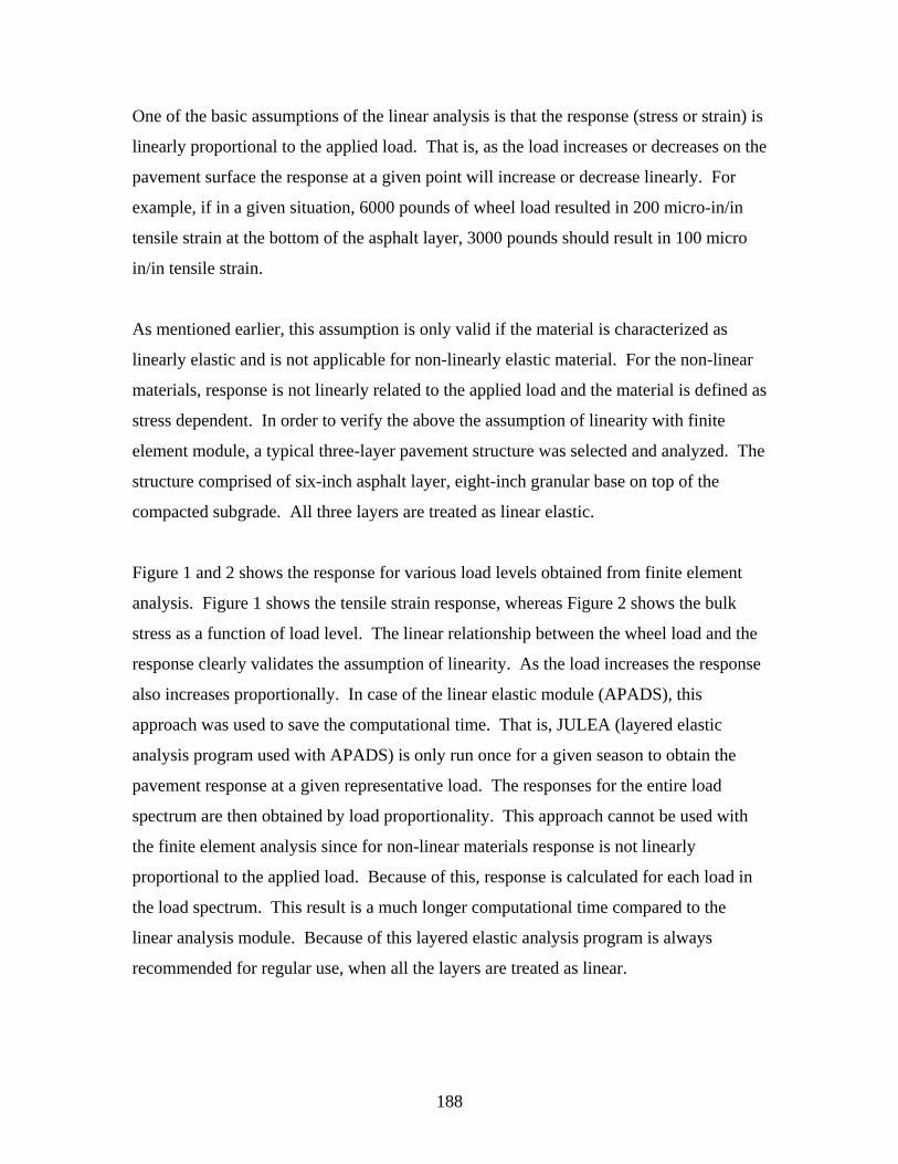
188

One of the basic assumptions of the linear analysis is that the response (stress or strain) is

linearly proportional to the applied load. That is, as the load increases or decreases on the

pavement surface the response at a given point will increase or decrease linearly. For

example, if in a given situation, 6000 pounds of wheel load resulted in 200 micro-in/in

tensile strain at the bottom of the asphalt layer, 3000 pounds should result in 100 micro

in/in tensile strain.

As mentioned earlier, this assumption is only valid if the material is characterized as

linearly elastic and is not applicable for non-linearly elastic material. For the non-linear

materials, response is not linearly related to the applied load and the material is defined as

stress dependent. In order to verify the above the assumption of linearity with finite

element module, a typical three-layer pavement structure was selected and analyzed. The

structure comprised of six-inch asphalt layer, eight-inch granular base on top of the

compacted subgrade. All three layers are treated as linear elastic.

Figure 1 and 2 shows the response for various load levels obtained from finite element

analysis. Figure 1 shows the tensile strain response, whereas Figure 2 shows the bulk

stress as a function of load level. The linear relationship between the wheel load and the

response clearly validates the assumption of linearity. As the load increases the response

also increases proportionally. In case of the linear elastic module (APADS), this

approach was used to save the computational time. That is, JULEA (layered elastic

analysis program used with APADS) is only run once for a given season to obtain the

pavement response at a given representative load. The responses for the entire load

spectrum are then obtained by load proportionality. This approach cannot be used with

the finite element analysis since for non-linear materials response is not linearly

proportional to the applied load. Because of this, response is calculated for each load in

the load spectrum. This result is a much longer computational time compared to the

linear analysis module. Because of this layered elastic analysis program is always

recommended for regular use, when all the layers are treated as linear.

189

0.00E+00

5.00E-06

1.00E-05

1.50E-05

2.00E-05

2.50E-05

3.00E-05

3.50E-05

0 1000 2000 3000 4000 5000 6000

Wheel Load (lbs)

Ten

sile

Str

ain

(in/in

)

Figure 1: Verification of Linearity with Tensile Strain Response at the Bottom of

Asphalt Layer for a Three Layer Pavement Structure

-1.5

-1.0

-0.5

0.0

0.5

1.0

1.5

0 1000 2000 3000 4000 5000 6000

Wheel Load (lbs)

Bul

k St

ress

(psi

)

Figure 2: Verification of Linearity with Bulk Stress Response in an Unbound Layer for a

Three layer Pavement Structure

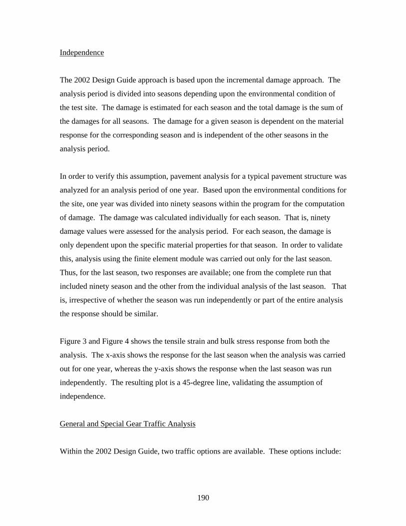
190

Independence

The 2002 Design Guide approach is based upon the incremental damage approach. The

analysis period is divided into seasons depending upon the environmental condition of

the test site. The damage is estimated for each season and the total damage is the sum of

the damages for all seasons. The damage for a given season is dependent on the material

response for the corresponding season and is independent of the other seasons in the

analysis period.

In order to verify this assumption, pavement analysis for a typical pavement structure was

analyzed for an analysis period of one year. Based upon the environmental conditions for

the site, one year was divided into ninety seasons within the program for the computation

of damage. The damage was calculated individually for each season. That is, ninety

damage values were assessed for the analysis period. For each season, the damage is

only dependent upon the specific material properties for that season. In order to validate

this, analysis using the finite element module was carried out only for the last season.

Thus, for the last season, two responses are available; one from the complete run that

included ninety season and the other from the individual analysis of the last season. That

is, irrespective of whether the season was run independently or part of the entire analysis

the response should be similar.

Figure 3 and Figure 4 shows the tensile strain and bulk stress response from both the

analysis. The x-axis shows the response for the last season when the analysis was carried

out for one year, whereas the y-axis shows the response when the last season was run

independently. The resulting plot is a 45-degree line, validating the assumption of

independence.

General and Special Gear Traffic Analysis

Within the 2002 Design Guide, two traffic options are available. These options include:

191

• General Traffic Analysis

• Special Gear Traffic Analysis

The “General Traffic” consists of regular highway traffic that included; single, tandem,

tridem and quad axle traffic configurations. This information is usually available from

the traffic studies. The second option available in the 2002 Design Guide is to analyze

the pavement structure for special gear types for special facilities, such as the port,

airports etc. In the special gear analysis, one of the gear configurations from regular

traffic could also be specified as special gear. Since the axle configuration from the

general traffic could also be used as a special gear configuration, it should yield the same

results as in the case of the general traffic, when used as a special gear within the

analysis.

In order to verify the above-mentioned assumption, standard tridem axle loading

configuration was chosen. The tridem axle was analyzed in the finite element module

first as a standard traffic loading and then as a user-defined vehicle. The dual wheel

spacing was 11.3” and the axle spacing was 49.2 inches. The tire load corresponded to

tridem axle load group # 10 (3125 lbs/wheel) with a contact radius of 2.87-inch, and a tire

pressure of 120 psi was used in the analysis.

Figure 5a shows the tensile strain response at two depths within the pavement system.

Surface strains are shown as z = 0, whereas strains at the bottom of asphalt layer are

shown as z = 6 inches. Figure 5b shows the comparison for the vertical strains (left side),

bulk and deviatoric stress (right side) for unbound layer. The legend “Special” in the

figures refers to the tridem axle that is treated as special axle within the program.

Whereas, “General” refers to the tridem axle that is treated as a general traffic within the

program. That is, the results for the tridem axles were obtained from two different

analysis routines and resulted into same response. These results show no difference in

the response between the two approaches.

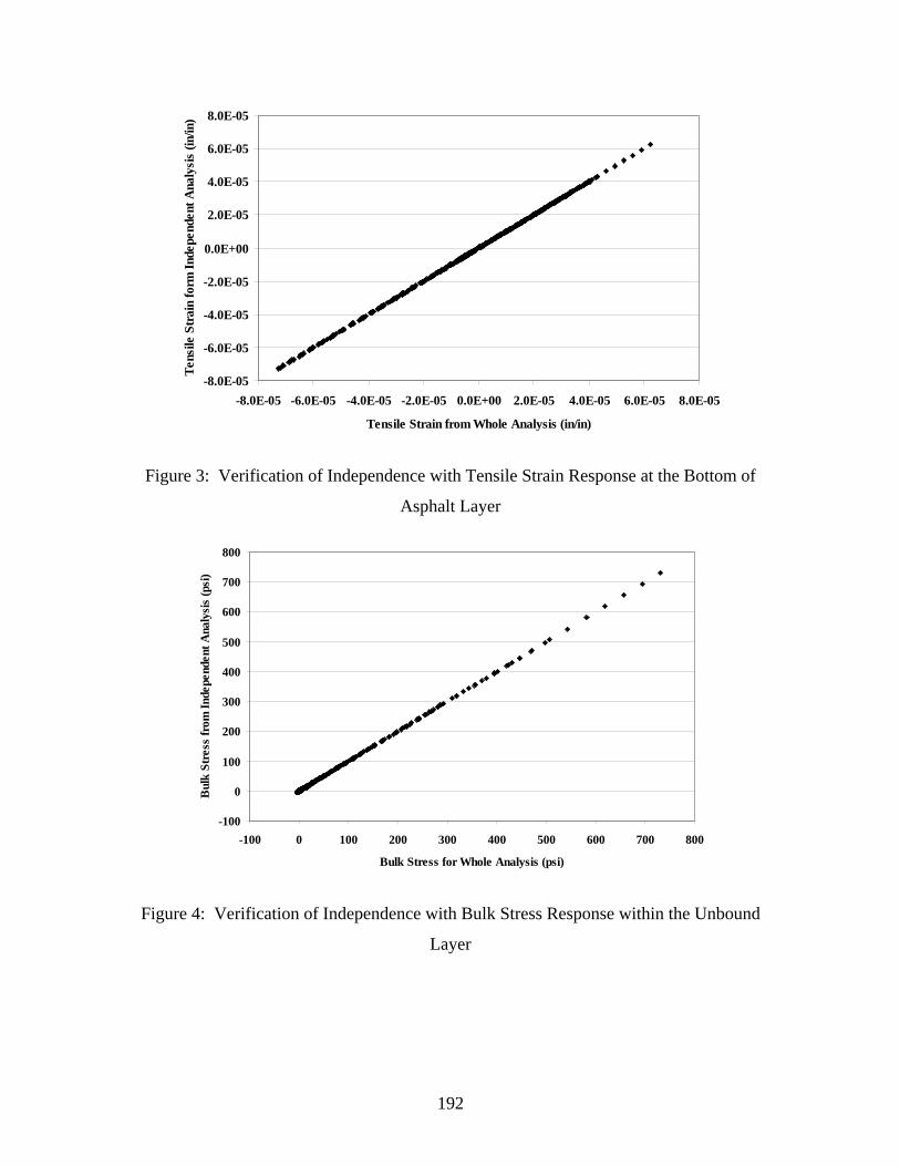
192

-8.0E-05

-6.0E-05

-4.0E-05

-2.0E-05

0.0E+00

2.0E-05

4.0E-05

6.0E-05

8.0E-05

-8.0E-05 -6.0E-05 -4.0E-05 -2.0E-05 0.0E+00 2.0E-05 4.0E-05 6.0E-05 8.0E-05

Tensile Strain from Whole Analysis (in/in)

Tens

ile S

trai

n fo

rm In

depe

nden

t Ana

lysi

s (in

/in)

Figure 3: Verification of Independence with Tensile Strain Response at the Bottom of

Asphalt Layer

-100

0

100

200

300

400

500

600

700

800

-100 0 100 200 300 400 500 600 700 800

Bulk Stress for Whole Analysis (psi)

Bul

k St

ress

from

Inde

pend

ent A

naly

sis

(psi

)

Figure 4: Verification of Independence with Bulk Stress Response within the Unbound

Layer

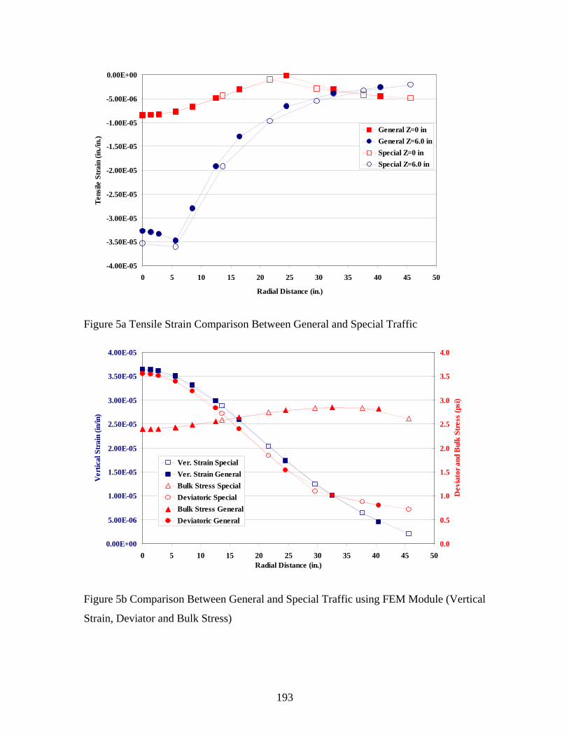
193

-4.00E-05

-3.50E-05

-3.00E-05

-2.50E-05

-2.00E-05

-1.50E-05

-1.00E-05

-5.00E-06

0.00E+00

0 5 10 15 20 25 30 35 40 45 50

Radial Distance (in.)

Tens

ile S

trai

n (in

./in.

)

General Z=0 inGeneral Z=6.0 inSpecial Z=0 inSpecial Z=6.0 in

Figure 5a Tensile Strain Comparison Between General and Special Traffic

0.00E+00

5.00E-06

1.00E-05

1.50E-05

2.00E-05

2.50E-05

3.00E-05

3.50E-05

4.00E-05

0 5 10 15 20 25 30 35 40 45 50Radial Distance (in.)

Ver

tical

Str

ain

(in/in

)

0.0

0.5

1.0

1.5

2.0

2.5

3.0

3.5

4.0

Dev

iato

r and

Bul

k St

ress

(psi

)Ver. Strain SpecialVer. Strain GeneralBulk Stress SpecialDeviatoric SpecialBulk Stress GeneralDeviatoric General

Figure 5b Comparison Between General and Special Traffic using FEM Module (Vertical

Strain, Deviator and Bulk Stress)

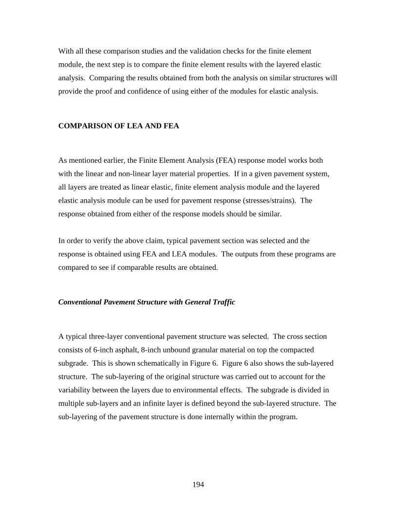
194

With all these comparison studies and the validation checks for the finite element

module, the next step is to compare the finite element results with the layered elastic

analysis. Comparing the results obtained from both the analysis on similar structures will

provide the proof and confidence of using either of the modules for elastic analysis.

COMPARISON OF LEA AND FEA

As mentioned earlier, the Finite Element Analysis (FEA) response model works both

with the linear and non-linear layer material properties. If in a given pavement system,

all layers are treated as linear elastic, finite element analysis module and the layered

elastic analysis module can be used for pavement response (stresses/strains). The

response obtained from either of the response models should be similar.

In order to verify the above claim, typical pavement section was selected and the

response is obtained using FEA and LEA modules. The outputs from these programs are

compared to see if comparable results are obtained.

Conventional Pavement Structure with General Traffic

A typical three-layer conventional pavement structure was selected. The cross section

consists of 6-inch asphalt, 8-inch unbound granular material on top the compacted

subgrade. This is shown schematically in Figure 6. Figure 6 also shows the sub-layered

structure. The sub-layering of the original structure was carried out to account for the

variability between the layers due to environmental effects. The subgrade is divided in

multiple sub-layers and an infinite layer is defined beyond the sub-layered structure. The

sub-layering of the pavement structure is done internally within the program.

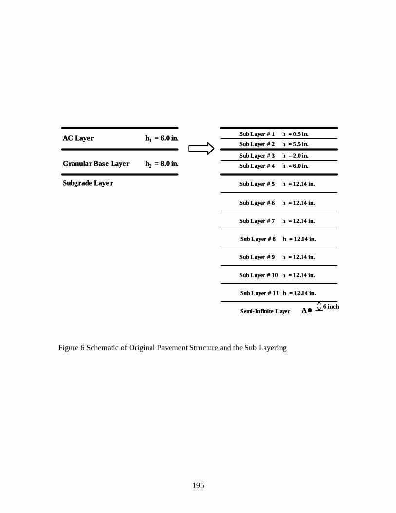
195

h1 = 6.0 in.AC Layer

Granular Base Layer

Subgrade Layer

h2 = 8.0 in.

Sub Layer # 1 h = 0.5 in.

Sub Layer # 2 h = 5.5 in.

Sub Layer # 3 h = 2.0 in.

Sub Layer # 4 h = 6.0 in.

Sub Layer # 5 h = 12.14 in.

Sub Layer # 6 h = 12.14 in.

Sub Layer # 7 h = 12.14 in.

Sub Layer # 8 h = 12.14 in.

Sub Layer # 9 h = 12.14 in.

Sub Layer # 10 h = 12.14 in.

Sub Layer # 11 h = 12.14 in.

Semi-Infinite Layer6 inchA

h1 = 6.0 in.AC Layer

Granular Base Layer

Subgrade Layer

h2 = 8.0 in.

Sub Layer # 1 h = 0.5 in.

Sub Layer # 2 h = 5.5 in.

Sub Layer # 3 h = 2.0 in.

Sub Layer # 4 h = 6.0 in.

Sub Layer # 5 h = 12.14 in.

Sub Layer # 6 h = 12.14 in.

Sub Layer # 7 h = 12.14 in.

Sub Layer # 8 h = 12.14 in.

Sub Layer # 9 h = 12.14 in.

Sub Layer # 10 h = 12.14 in.

Sub Layer # 11 h = 12.14 in.

Semi-Infinite Layer6 inchA

Figure 6 Schematic of Original Pavement Structure and the Sub Layering

196

For each of these layers the response is computed using the finite element as well as the

layered elastic analysis module. The response parameters obtained from these two

modules include:

1. Tensile strain at bottom of stabilized (asphalt) layers

2. Vertical strain at mid-depth of each layer

3. Bulk stress at mid-depth of each layer

4. Deviator stress at mid-depth of each layer

The response parameters obtained are used for the determination of distresses such as the

fatigue and permanent deformation in the respective layers. It is important that the

responses from the two approaches result in similar values, since this will directly effect

the computation of the distresses and performance evaluation.

Figure 7a and Figure 7b shows the comparison of the FEA and the LEA for the tensile

strains at three depths. Figure 7a shows the computed strain values form both the finite

element and the layered analysis module (APADS), whereas Figure 7b shows difference

in the strain values. It shows that the computed strains are very close and in most cases

the difference in the tensile strain values is less than 2-micro-in/in. This small difference

is due to the approximation used in the finite element analysis or the mathematical

approach used in both the analysis.

One other observations made is that relatively higher difference was observed at the outer

edge of the tire (radial distance = 8.5 inches) at the surface. This was expected since the

sharp changes in the stress and strain distributions here are difficult to track in the FEA

calculations. The errors are generally quite small, and the extent of the error region would

also be expected to be quite small. Note that in this region our modeling idealization of a

uniform tire pressure distribution is also in error; the errors from neglecting the actual tire

pressure distribution is probably greater than the errors from the finite element

interpolations in this region. In addition, strains in this region are always going to be

compressive at the surface.

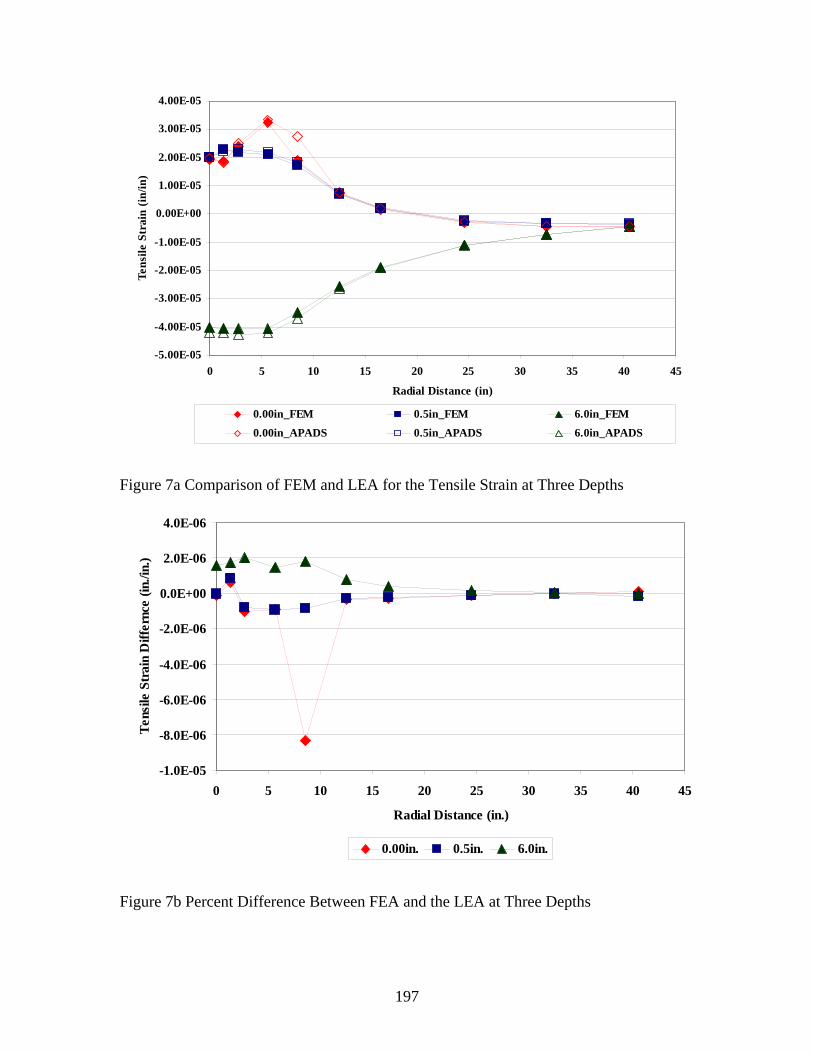
197

-5.00E-05

-4.00E-05

-3.00E-05

-2.00E-05

-1.00E-05

0.00E+00

1.00E-05

2.00E-05

3.00E-05

4.00E-05

0 5 10 15 20 25 30 35 40 45

Radial Distance (in)

Tens

ile S

trai

n (in

/in)

0.00in_FEM 0.5in_FEM 6.0in_FEM

0.00in_APADS 0.5in_APADS 6.0in_APADS

Figure 7a Comparison of FEM and LEA for the Tensile Strain at Three Depths

-1.0E-05

-8.0E-06

-6.0E-06

-4.0E-06

-2.0E-06

0.0E+00

2.0E-06

4.0E-06

0 5 10 15 20 25 30 35 40 45

Radial Distance (in.)

Tens

ile S

trai

n D

iffer

nce

(in./i

n.)

0.00in. 0.5in. 6.0in.

Figure 7b Percent Difference Between FEA and the LEA at Three Depths

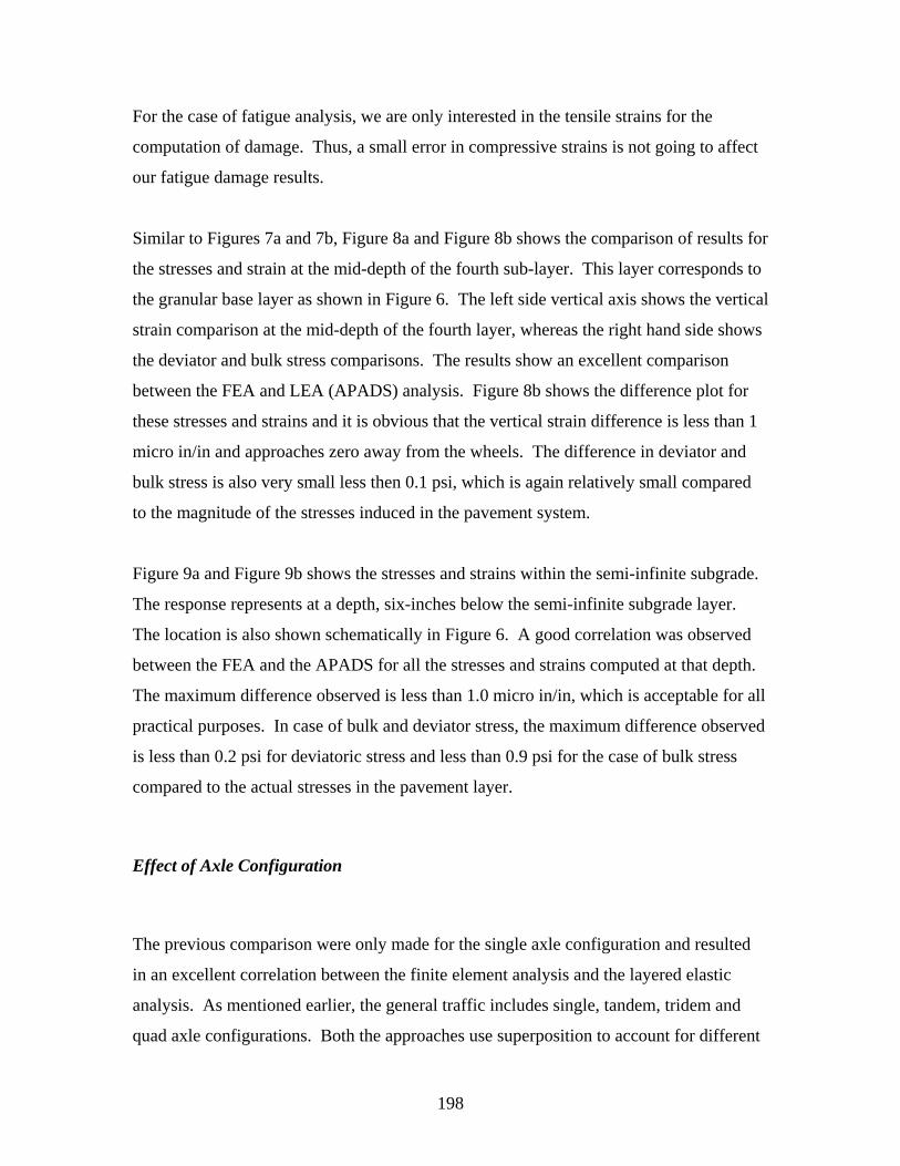
198

For the case of fatigue analysis, we are only interested in the tensile strains for the

computation of damage. Thus, a small error in compressive strains is not going to affect

our fatigue damage results.

Similar to Figures 7a and 7b, Figure 8a and Figure 8b shows the comparison of results for

the stresses and strain at the mid-depth of the fourth sub-layer. This layer corresponds to

the granular base layer as shown in Figure 6. The left side vertical axis shows the vertical

strain comparison at the mid-depth of the fourth layer, whereas the right hand side shows

the deviator and bulk stress comparisons. The results show an excellent comparison

between the FEA and LEA (APADS) analysis. Figure 8b shows the difference plot for

these stresses and strains and it is obvious that the vertical strain difference is less than 1

micro in/in and approaches zero away from the wheels. The difference in deviator and

bulk stress is also very small less then 0.1 psi, which is again relatively small compared

to the magnitude of the stresses induced in the pavement system.

Figure 9a and Figure 9b shows the stresses and strains within the semi-infinite subgrade.

The response represents at a depth, six-inches below the semi-infinite subgrade layer.

The location is also shown schematically in Figure 6. A good correlation was observed

between the FEA and the APADS for all the stresses and strains computed at that depth.

The maximum difference observed is less than 1.0 micro in/in, which is acceptable for all

practical purposes. In case of bulk and deviator stress, the maximum difference observed

is less than 0.2 psi for deviatoric stress and less than 0.9 psi for the case of bulk stress

compared to the actual stresses in the pavement layer.

Effect of Axle Configuration

The previous comparison were only made for the single axle configuration and resulted

in an excellent correlation between the finite element analysis and the layered elastic

analysis. As mentioned earlier, the general traffic includes single, tandem, tridem and

quad axle configurations. Both the approaches use superposition to account for different

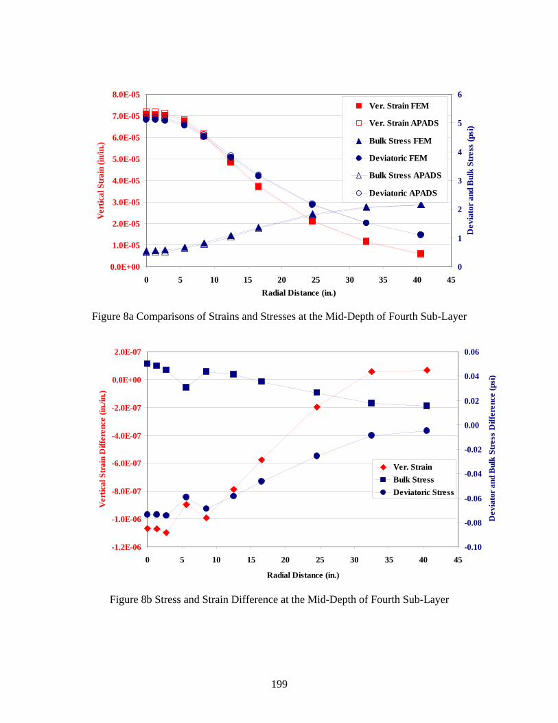
199

0.0E+00

1.0E-05

2.0E-05

3.0E-05

4.0E-05

5.0E-05

6.0E-05

7.0E-05

8.0E-05

0 5 10 15 20 25 30 35 40 45Radial Distance (in.)

Ver

tical

Str

ain

(in/in

.)

0

1

2

3

4

5

6

Dev

iato

r and

Bul

k St

ress

(psi

)

Ver. Strain FEM

Ver. Strain APADS

Bulk Stress FEM

Deviatoric FEM

Bulk Stress APADS

Deviatoric APADS

Figure 8a Comparisons of Strains and Stresses at the Mid-Depth of Fourth Sub-Layer

-1.2E-06

-1.0E-06

-8.0E-07

-6.0E-07

-4.0E-07

-2.0E-07

0.0E+00

2.0E-07

0 5 10 15 20 25 30 35 40 45

Radial Distance (in.)

Ver

tical

Str

ain

Diff

eren

ce (i

n./in

.)

-0.10

-0.08

-0.06

-0.04

-0.02

0.00

0.02

0.04

0.06

Dev

iato

r and

Bul

k St

ress

Diff

eren

ce (p

si)

Ver. StrainBulk StressDeviatoric Stress

Figure 8b Stress and Strain Difference at the Mid-Depth of Fourth Sub-Layer

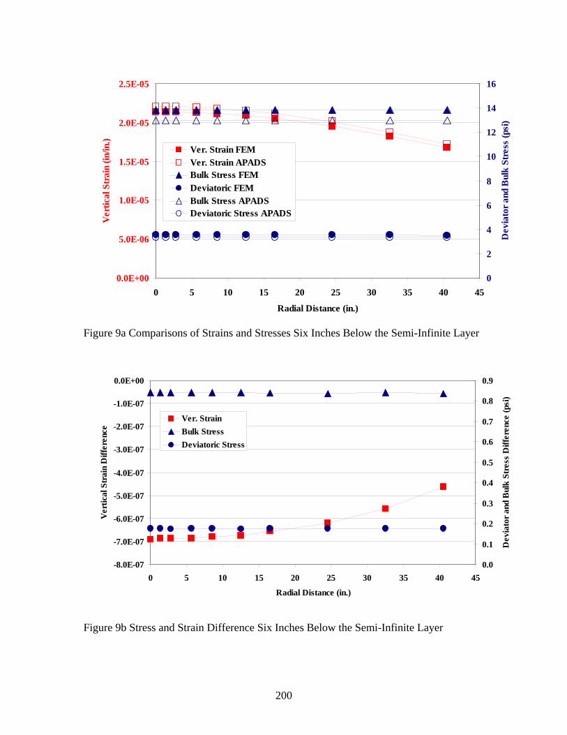
200

0.0E+00

5.0E-06

1.0E-05

1.5E-05

2.0E-05

2.5E-05

0 5 10 15 20 25 30 35 40 45

Radial Distance (in.)

Ver

tical

Str

ain

(in/in

.)

0

2

4

6

8

10

12

14

16

Dev

iato

r and

Bul

k St

ress

(psi

)

Ver. Strain FEMVer. Strain APADSBulk Stress FEMDeviatoric FEMBulk Stress APADSDeviatoric Stress APADS

Figure 9a Comparisons of Strains and Stresses Six Inches Below the Semi-Infinite Layer

-8.0E-07

-7.0E-07

-6.0E-07

-5.0E-07

-4.0E-07

-3.0E-07

-2.0E-07

-1.0E-07

0.0E+00

0 5 10 15 20 25 30 35 40 45

Radial Distance (in.)

Ver

tical

Str

ain

Diff

eren

ce

0.0

0.1

0.2

0.3

0.4

0.5

0.6

0.7

0.8

0.9

Dev

iato

r and

Bul

k St

ress

Diff

eren

ce (p

si)

Ver. StrainBulk StressDeviatoric Stress

Figure 9b Stress and Strain Difference Six Inches Below the Semi-Infinite Layer

201

axle types. In order to check the compatibility in the superposition approach, a pavement

structure shown in Figure 6 was analyzed and compared for different axle configurations.

The comparison results for tandem, tridem and quad axle configurations are compared

between the finite element and the layered elastic analysis. As mentioned earlier, the

response for the elastic layered analysis was carried out at a representation load for a

constant radius of contact. The response at other load levels in the spectrum is then

calculated by using load proportions. For this example, the representative load for the

LEA (APADS) was 3125 pounds per wheel and the tire pressure used was 120 psi. This

corresponds to load group # 11 for tandem axle, load group # 10 for tridem axle and load

group # 14 for quad axle. The response from these load groups from the FEA was

obtained and compared to the response from LEA.

Figure 10a shows tensile strain values at the bottom of the asphalt layer (second sub-

layer). Results were plotted for tandem, tridem and quad axle configurations. As shown

in Figure 10b, the maximum difference between the two analyses was less than 2 micro

in/in and is considered to be acceptable. It should be realized that the maximum value of

error occurred at a radial distance less than 8.5 inches from the center or close to the

wheels. The average strain value is between 35 to 40 micro in/in and an error of 2 micro

in/in is insignificant. This shows that the axle configuration is insensitive to the

difference between the finite element and the layered elastic analysis.

Similar to the results shown in Figure 10a and 10b, comparison was made for the bulk

stress in unbound granular base (sub-layer #4), and the results are shown in Figure 11a

and Figure 11b. The comparison between the finite element and the layered elastic

analysis resulted in excellent results. The maximum error or difference between the two

analysis approaches was less than 0.15 psi, which is insignificant compared to the amount

of stress in the pavement system at this depth.

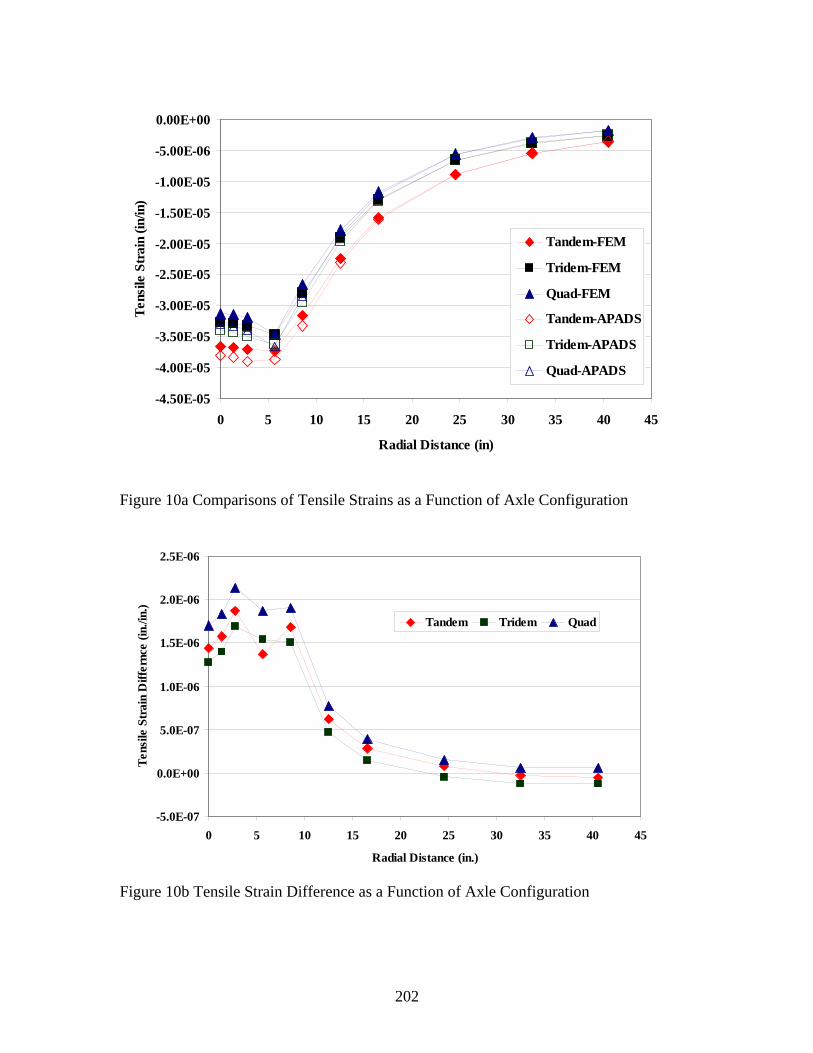
202

-4.50E-05

-4.00E-05

-3.50E-05

-3.00E-05

-2.50E-05

-2.00E-05

-1.50E-05

-1.00E-05

-5.00E-06

0.00E+00

0 5 10 15 20 25 30 35 40 45

Radial Distance (in)

Tens

ile S

trai

n (in

/in)

Tandem-FEM

Tridem-FEM

Quad-FEM

Tandem-APADS

Tridem-APADS

Quad-APADS

Figure 10a Comparisons of Tensile Strains as a Function of Axle Configuration

-5.0E-07

0.0E+00

5.0E-07

1.0E-06

1.5E-06

2.0E-06

2.5E-06

0 5 10 15 20 25 30 35 40 45

Radial Distance (in.)

Tens

ile S

trai

n D

iffer

nce

(in./i

n.)

Tandem Tridem Quad

Figure 10b Tensile Strain Difference as a Function of Axle Configuration

203

0.0

0.5

1.0

1.5

2.0

2.5

3.0

3.5

0 5 10 15 20 25 30 35 40 45

Radial Distance (in.)

Bul

k St

ress

(psi

)

Tandem-FEMTridem-FEMQuad-FEMTandem-APADSTridem-APADSQuad-APADS

Figure 11a Comparisons of Bulk Stress as a Function of Axle Configuration

0.00

0.02

0.04

0.06

0.08

0.10

0.12

0.14

0 5 10 15 20 25 30 35 40 45Radial Distance (in.)

Stre

ss D

iffer

ence

(psi

)

TandemTridemQuad

Figure 11b Bulk Stress Difference as a Function of Axle Configuration

204

Special Gear Configuration

Another comparison study was carried out with a special gear assembly. Figure 12

shows the special gear assembly that was used for comparing the results for the finite

element and layered elastic analysis. The importance of this example is to also check the

superposition capabilities of both the analysis. Load on each wheel was 19620 pounds

with a tire pressure of 180 psi, resulting in a radius of contact of 5.89 inches. The gear

dimensions are schematically shown in Figure 12.

Figure 13a and Figure 13b shows comparison of the tensile strains in the asphalt layer.

The results show good correlation between the finite element and the linear elastic

analysis (APADS). Results at a depth of six inches resulted in the best correlation,

however at a depth of z=0 and z=0.5 inches the difference in strains is less than 6 micro

in/in. This was expected since the sharp changes in the stress and strain distributions here

are difficult to track in the FEA calculations. The errors are generally quite small, and the

extent of the error region would also be expected to be quite small. In addition, the actual

values of tensile strain at the surface are also very small, which are considered as

insignificant for fatigue damage.

Finally, Figure 14a and Figure 14b shows the stresses and strains in the unbound layer

(sub-layer #4, Figure 6). Although the maximum difference in the vertical is close to 14

micro in/in, but this is considered to be insignificant when compared to the actual strain

in that layer. The magnitude of tensile strain is close to 300 micro in/in. This difference

is mainly attributed to the mathematical approximations used in the finite element

module. When considering the deviatoric and the bulk stress, the differences are

insignificant compared to the amount the stress in the pavement layer. The maximum

error in the deviatoric stress is 1.0 psi, when the actual stress is close to 20 psi. This

small difference is considered to be insignificant for all practical purposes.

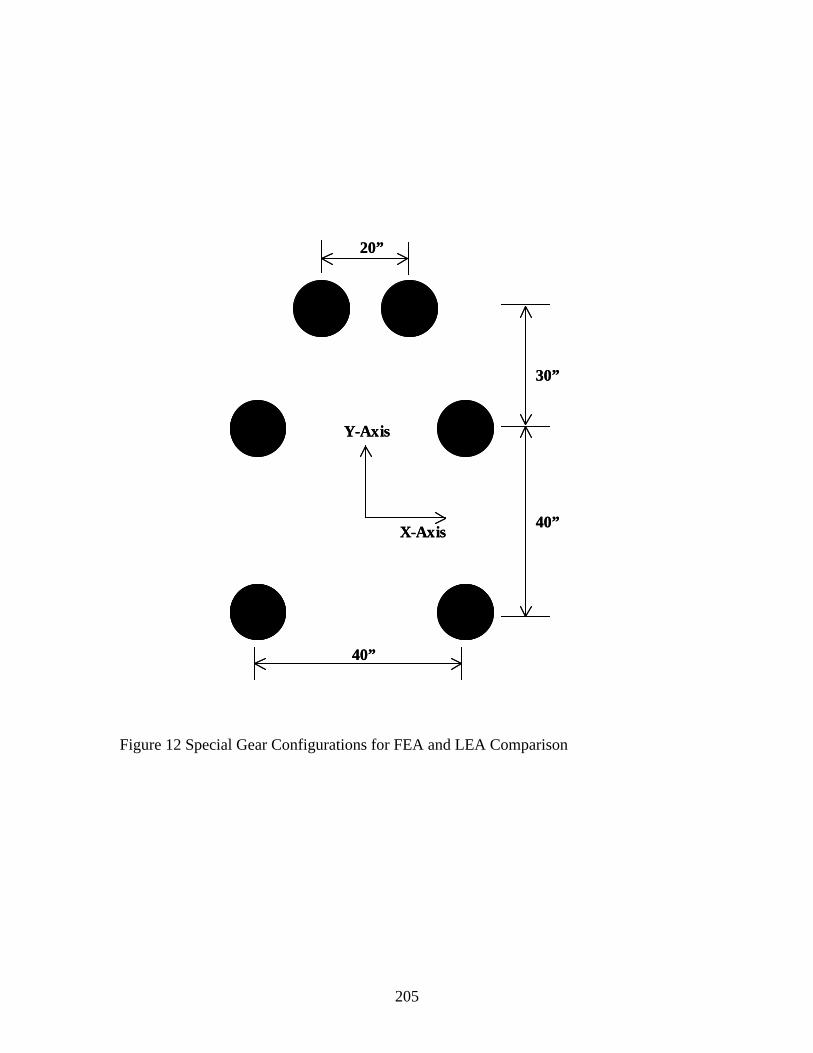
205

40”

X-Axis

Y-Axis

40”

30”

20”

40”

X-Axis

Y-Axis

40”

30”

20”

Figure 12 Special Gear Configurations for FEA and LEA Comparison

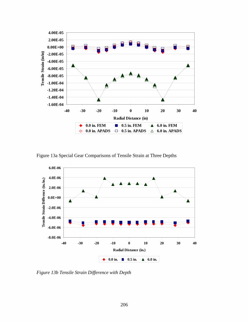
206

-1.60E-04

-1.40E-04

-1.20E-04

-1.00E-04

-8.00E-05

-6.00E-05

-4.00E-05

-2.00E-05

0.00E+00

2.00E-05

4.00E-05

-40 -30 -20 -10 0 10 20 30 40

Radial Distance (in)

Tens

ile S

trai

n (in

/in)

0.0 in. FEM 0.5 in. FEM 6.0 in. FEM0.0 in. APADS 0.5 in. APADS 6.0 in. APADS

Figure 13a Special Gear Comparisons of Tensile Strain at Three Depths

-8.0E-06

-6.0E-06

-4.0E-06

-2.0E-06

0.0E+00

2.0E-06

4.0E-06

6.0E-06

-40 -30 -20 -10 0 10 20 30 40

Radial Distance (in.)

Tens

ile S

trai

n D

iffer

nce

(in./i

n.)

0.0 in. 0.5 in. 6.0 in.

Figure 13b Tensile Strain Difference with Depth

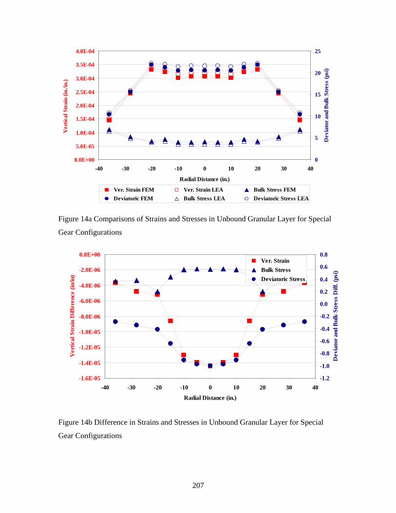
207

0.0E+00

5.0E-05

1.0E-04

1.5E-04

2.0E-04

2.5E-04

3.0E-04

3.5E-04

4.0E-04

-40 -30 -20 -10 0 10 20 30 40

Radial Distance (in.)

Ver

tical

Str

ain

(in./i

n.)

0

5

10

15

20

25

Dev

iato

r and

Bul

k St

ress

(psi

)

Ver. Strain FEM Ver. Strain LEA Bulk Stress FEMDeviatoric FEM Bulk Stress LEA Deviatoric Stress LEA

Figure 14a Comparisons of Strains and Stresses in Unbound Granular Layer for Special

Gear Configurations

-1.6E-05

-1.4E-05

-1.2E-05

-1.0E-05

-8.0E-06

-6.0E-06

-4.0E-06

-2.0E-06

0.0E+00

-40 -30 -20 -10 0 10 20 30 40

Radial Distance (in.)

Ver

tical

Str

ain

Diff

eren

ce (i

n/in

)

-1.2

-1.0

-0.8

-0.6

-0.4

-0.2

0.0

0.2

0.4

0.6

0.8

Dev

iato

r and

Bul

k St

ress

Diff

. (ps

i)

Ver. StrainBulk StressDeviatoric Stress

Figure 14b Difference in Strains and Stresses in Unbound Granular Layer for Special

Gear Configurations

208

SUMMARY

Accurate pavement performance prediction is widely recognized by pavement

community as one of the most important, complex and difficult task to pursue. The

important of such a goal cannot be overemphasized because this will result in the saving

of millions of dollars. Proper selection of pavement materials and layer thickness can be

optimized based upon performance-based specification. The basic requirement for this is

the availability of the accurate pavement performance prediction methodology. This can

be accomplished if the materials in the pavement system can be by reasonable

characterized by the use of constitutive models. That is, the relationship of stress and

strain can be established for all paving materials. Once a good estimate of response is

available that can be used for distress predictions and the development of performance

based specifications.

Within the 2002 Design Guide the response for the layered elastic system can be obtained

either by finite element analysis or by the use of layered elastic analysis, which is based

upon theory of elasticity. It is important that the results obtained from both the analysis

are comparable. This documents compares the results of the finite element analysis with

that of layered elastic analysis (APADS). Following general conclusions were made

based on the work presented in this report.

1. Finite element module was verified for various analyses. This included; linearity

check, independence of results and comparison of general and special traffic

analysis. It was found, for a linear elastic system the response is proportional to

load. The results of seasons are independent of the other seasons and finally the

results from the special traffic are comparable with the general traffic analysis.

2. Comparison between finite element and layered elastic analysis was made for

different situations. This included comparing; tensile strains, vertical strains, bulk

stress and the deviatoric stress. The results from this comparison showed good

correlation between the finite element and the layered elastic analysis solution.

209

3. A small difference between the two analyses is the result of the mathematical

approach used by the two analyses. The finite element results are highly

dependent upon the mesh size and convergence criteria.

4. In some situations the difference between the two analyses is relatively larger.

This occurs when the magnitude of the response is also very large. That is, an

error of 1.0 psi, in bulk stress is insignificant if the total bulk stress on the system

is 30 psi. However, an error of 10 psi, is significant if the total bulk stress is 30

psi. It is important to compare the difference with the amount of the response.

5. In some situations, error close to the surface or especially close to the tires is

larger compared to the locations away from the tires and at greater depths. This

was expected since the sharp changes in the stress and strain distributions close to

the tire are difficult to track in the FEA calculations. The errors are generally

quite small, and the extent of the error region would also be expected to be quite

small. Note that in this region our modeling idealization of a uniform tire

pressure distribution is also in error; the errors from neglecting the actual tire

pressure distribution is probably greater than the errors from the finite element

interpolations in this region.

_____________________________________