Of Mice and Merchants: Trade and Growth in the Iron...
55
Of Mice and Merchants: Trade and Growth in the Iron Age Stephan Maurer * , J¨orn-Steffen Pischke † , Ferdinand Rauch ‡ May 11, 2017 Abstract We study the causal connection between trade and development using one of the earliest massive trade expansions in prehistory: the first systematic crossing of open seas in the Mediterranean during the time of the Phoenicians. For each point on the coast, we construct the ease with which other points can be reached by crossing open water. This connectivity differs depending on the shape of the coast, the location of islands, and the distance to the opposing shore. We find an association between better connected locations and archaeological sites during the Iron Age, at a time when sailors began to cross open water very routinely and on a big scale. We corroborate these findings at the level of the world. JEL classification: F14, N7, O47 Keywords: Urbanization, locational fundamentals, trade * LSE and CEP, [email protected] † LSE and CEP, [email protected] ‡ Oxford and CEP, [email protected]. We thank Jan Bakker and Juan Pradera for excellent research assistance, and David Abulafia, Tim Besley, Andrew Bevan, Francesco Caselli, Jeremiah Dittmar, Avner Greif, Carl Knappett, Andrea Matranga, Guy Michaels, Dennis Novy, Luigi Pascali, Dominic Rathbone, Tanner Regan, Corinna Riva, Susan Sherratt, Pedro CL Souza, Peter Temin, John van Reenen, Ruth Whitehouse, and participants at various seminars and conferences for their helpful comments and suggestions. 1
-
Upload
duongkhuong -
Category
Documents
-
view
215 -
download
0
Transcript of Of Mice and Merchants: Trade and Growth in the Iron...
Of Mice and MerchantsTrade and Growth in the Iron Age
Stephan Maurerlowast Jorn-Steffen Pischkedagger Ferdinand RauchDagger
May 11 2017
Abstract
We study the causal connection between trade and development using one of theearliest massive trade expansions in prehistory the first systematic crossing of openseas in the Mediterranean during the time of the Phoenicians For each point onthe coast we construct the ease with which other points can be reached by crossingopen water This connectivity differs depending on the shape of the coast thelocation of islands and the distance to the opposing shore We find an associationbetween better connected locations and archaeological sites during the Iron Age ata time when sailors began to cross open water very routinely and on a big scale Wecorroborate these findings at the level of the world
JEL classification F14 N7 O47
Keywords Urbanization locational fundamentals trade
lowastLSE and CEP semaurerlseacukdaggerLSE and CEP spischkelseacukDaggerOxford and CEP ferdinandraucheconomicsoxacuk We thank Jan Bakker and Juan Pradera
for excellent research assistance and David Abulafia Tim Besley Andrew Bevan Francesco CaselliJeremiah Dittmar Avner Greif Carl Knappett Andrea Matranga Guy Michaels Dennis Novy LuigiPascali Dominic Rathbone Tanner Regan Corinna Riva Susan Sherratt Pedro CL Souza Peter TeminJohn van Reenen Ruth Whitehouse and participants at various seminars and conferences for their helpfulcomments and suggestions
1
1 Introduction
We investigate to what degree trading opportunities affected economic development at an
early juncture of human history In addition to factor accumulation and technical change
Smithian growth due to exchange and specialization is one of the fundamental sources of
growth An emerging literature on the topic is beginning to provide compelling empirical
evidence for a causal link from trade to growth We contribute to this literature and focus
on one of the earliest trade expansions in pre-history the systematic crossing of open
seas in the Mediterranean at the time of the Phoenicians from about 900 BC We relate
trading opportunities which we capture through the connectedness of points along the
coast to early development as measured by the presence of archaeological sites We find
that locational advantages for sea trade matter for the foundation of Iron Age cities and
settlements and thus helped shape the development of the Mediterranean region and the
world
A location with more potential trading partners should have an advantage if trade is
important for development The particular shape of a coast has little influence over how
many neighboring points can be reached from a starting location within a certain distance
as long as ships sail mainly close to the coast However once sailors begin to cross open
seas coastal geography becomes more important Some coastal points are in the reach of
many neighbors while other can reach only few The general shape of the coast and the
location of islands matters for this We capture these geographic differences by dividing
the Mediterranean coast into grid cells and calculating how many other cells can be
reached within a certain distance Parts of the Mediterranean are highly advantaged by
their geography eg the island-dotted Aegean and the ldquowaist of the Mediterraneanrdquo
at southern Italy Sicily and modern Tunisia Other areas are less well connected like
most of the North African coast parts of Iberia and southern France and the Levantine
coast
2
We relate our measure of connectivity to the number of archaeological sites found near
any particular coastal grid point This is our proxy for economic development It is based
on the assumption that more human economic activity leads to more settlements and
particularly towns and cities While these expand and multiply there are more traces
in the archaeological record We find a pronounced relationship between connectivity
and development in our data set for the Iron Age around 750 BC when the Phoenicians
had begun to systematically traverse the open sea using various different data sources
for sites We find a weaker and less consistent relationship between connectivity and
sites for earlier periods This is consistent with the idea that earlier voyages occurred
maybe at intermediate distances at some frequency already during the Bronze Age Our
interpretation of the results suggests that the relationship between coastal geography and
settlement density once established in the Iron Age persists through the classical period
This is consistent with a large literature in economic geography on the persistence of
city locations While our main results pertain to the Mediterranean where we have good
information on archaeological sites we also corroborate our findings at a world scale using
population data for 1 AD from McEvedy and Jones (1978) as outcome
Humans have obtained goods from far away locations for many millennia While some
of the early trade involved materials useful for tools (like the obsidian trade studied by
Dixon Cann and Renfrew 1968) as soon as societies became more differentiated a large
part of this early trade involved luxury goods doubtlessly consumed by the elites Such
trade might have raised the utility of the beneficiaries but it is much less clear whether
it affected productivity as well Although we are unable to measure trade directly our
work sheds some light on this question Since trade seems to have affected the growth of
settlements even at an early juncture this suggests that it was productivity enhancing The
view that trade played an important role in early development has recently been gaining
ground among economic historians see eg Temin (2006) for the Iron Age Mediterranean
Algaze (2008) for Mesopotamia and Temin (2013) for Ancient Rome
3
Our approach avoids issues of reverse causality and many confounders by using a geog-
raphy based instrument for trade In fact we do not observe trade itself but effectively
estimate a reduced form relationship relating opportunities for trade directly to economic
development This means that we do not necessarily isolate the effect of the exchange of
goods per se Our results could be driven by migration or the spread of ideas as well and
when we talk about ldquotraderdquo we interpret it in this broad sense We do believe that coastal
connectivity captures effects due to maritime connections It is difficult to imagine any
other channel why geography would matter in this particular manner and we show that
our results are not driven by a variety of other geographic conditions
Since we do not use any trade data we avoid many of the measurement issues related
to trade We measure trading opportunities and development at a fine geographic scale
hence avoiding issues of aggregation to a coarse country level Both our measure of
connectedness and our outcome variable are doubtlessly extremely crude proxies of both
trading opportunities and of economic development This will likely bias us against finding
any relationship and hence makes our results only more remarkable
The periods we study the Bronze and Iron Ages were characterized by the rise and decline
of many cultures and local concentrations of economic activity Many settlements and
cities rose during this period only to often disappear again This means that there were
ample opportunities for new locations to rise to prominence while path dependence and
hysteresis may have played less role compared to later ages The political organization of
the Mediterranean world prior to the Romans was mostly local The Egyptian Kingdoms
are the main exception to this rule but Egypt was mostly focused on the Nile and less
engaged in the Mediterranean As a result institutional factors were less important during
the period we study
There is a large literature on trade and growth Canonical studies are the investigations by
Frankel and Romer (1999) and Redding and Venables (2004) These papers use distance
4
from markets and connectivity as measured by gravity relationships to capture the ease
with which potential trading partners can be reached However these measures do not
rely purely on geography but conflate economic outcomes like population and output
which are themselves affected by the development process
The more recent literature has circumvented this by analyzing exogenous events related to
changes in trade Most similar to our study are a series of papers which also exploit new
trade relationships arising from discoveries the opening of new trade routes and tech-
nological change Acemoglu Johnson and Robinson (2005) link Atlantic trade starting
around 1500 AD to the ensuing shift in the focus of economic activity in Europe from the
south and center of the continent to the Atlantic periphery Redding and Sturm (2008)
focus on the natural experiment created by the division and reunification in Germany
which changed the access to other markets sharply for some locations but not others
Various papers exploit the availability of new transport technologies Feyrer (2009) uses
air transport Donaldson (forthcoming) and Donaldson and Hornbeck (2016) use rail-
roads and Pascali (forthcoming) steam ships These papers generally find that regions
whose trading opportunities improved disproportionately saw larger income growth That
we find similar results for a much earlier trade expansion suggests that the productivity
benefits of trade have been pervasive throughout history
Our paper also relates to a literature on how changes in locational fundamentals shape
the location of cities (Davis and Weinstein 2002 Bleakley and Lin 2012 Bosker and
Buringh 2017 Michaels and Rauch forthcoming) Our contribution to this literature is
to give evidence on one of the most important locational fundamentals market access
In a world with multiple modes of transport for the transportation of different goods it
is typically hard to measure market access and changes of market access of a city Our
measure relates to a world where much long distance trade took place on boats which
makes it easier to isolate a measure of market access
5
Also closely related is the paper by Ashraf and Galor (2011a) They relate population
density in various periods to the relative geographic isolation of a particular area Their
interest is in the impact of cultural diversity on the development process and they view
geographic isolation effectively as an instrument for cultural homogeneity Similar to our
measure their geographic isolation measure is a measure of connectivity of various points
around the world They find that better connected (ie less isolated) countries have lower
population densities for every period from 1 to 1500 AD which is the opposite of our
result Our approach differs from Ashraf and Galor (2011a) in that we only look at coasts
and not inland locations They control for distance to waterways in their regressions a
variable that is strongly positively correlated with population density Hence our results
are not in conflict with theirs
Our paper is also related to a number of studies on pre-historic Mediterranean connectivity
and seafaring McEvedy (1967) creates a measure of ldquolittoral zonesrdquo using coastal shapes
He produces a map which closely resembles the one we obtain from our connectivity
measure but does not relate geography directly to seafaring This is done by Broodbank
(2006) who overlays the connectivity map with archaeological evidence of the earliest
sea-crossings up to the end of the last Ice Age He interprets the connections as nursery
conditions for the early development of nautical skills rather than as market access as
we do for the later Bronze and Iron Ages Also related is a literature in archaeology using
network models connecting archaeological sites Knappett Evans and Rivers (2008) is an
excellent example for the Bronze Age Aegean None of these papers relate to the changes
arising from open sea-crossings which is the focus of our analysis Temin (2006) discusses
the Iron Age Mediterranean through the lens of comparative advantage trade but offers
no quantitative evidence as we do
6
2 Brief history of ancient seafaring in the Mediter-
ranean
The Mediterranean is a unique geographic space The large inland sea is protected from
the open oceans by the Strait of Gibraltar The tectonics of the area the African plate
descending under the Eurasian one have created a rugged northern coast in Europe
and a much straighter one in North Africa Volcanic activity and the more than 3000
islands also tend to be concentrated towards the north The climatic conditions in the
Mediterranean are generally relatively favorable to agriculture particularly in the north
The Mediterranean is the only large inland sea with such a climate (Broodbank 2013) Its
east-west orientation facilitated the spread of agriculture from the Levant (Diamond 1997)
Despite these common features the size of the Mediterranean and an uneven distribution
of natural resources also implies great diversity Modern writers on the Mediterranean
most notably Horden and Purcell (2000) have stressed that the area consists of many
micro-regions Geography and climate make the Mediterranean prone to many risks such
as forest fires earthquakes plagues of locusts droughts floods and landslides As a
consequence trade networks that allow to moderate shocks are of great mutual interest
in the region and trade has played a central role since its early history1
Clear evidence of the first maritime activity of humans in the Mediterranean is elusive
Crossings to islands close to the mainland were apparently undertaken as far back as
30000 BC (Fontana Nuova in Sicily) In a careful review of the evidence Broodbank
(2006) dates more active seafaring to around 10000 BC based on the distribution of
obsidian (a volcanic rock) at sites separated by water (see Dixon Cann and Renfrew
1965 1968) This points to the existence of active sea-faring of hunter-gatherer societies
and suggests that boats must have traveled distances of 20-35 kilometers around that
1The following discussion mainly draws on Abulafia (2011) and Broodbank (2013)
7
time We have no evidence on the first boats but they were likely made from skin and
frame or dugout canoes
The beginning of agriculture around the Mediterranean happened in the Levant between
9500 BC and 8000 BC From there it spread initially to Anatolia and the Aegean Signs
of a fairly uniform Neolithic package of crops and domesticated animals can be found
throughout the Mediterranean The distribution of the earliest evidence of agriculture
which includes islands before reaching more peripheral parts of the mainland suggests a
maritime transmission channel
The Neolithic revolution did not reach Iberia until around 5500 BC By that time many
islands in the Aegean had been settled there is evidence for grain storage and metal
working began in the Balkans Because of the uneven distribution of ores metals soon
became part of long range transport Uncertainty must have been a reason for the for-
mation of networks both for insurance and exchange The first archaeological evidence of
a boat also stems from this period a dugout canoe about 10 m long at La Marmotta
north of Rome A replica proved seaworthy and allowed travel of 20 - 25 km per day in a
laden boat
The Levant which was home to the first cities remained a technological leader in the
region yet there is little evidence of sea-faring even during the Copper Age This changed
with the rise of large scale societies in Mesopotamia and Egypt Inequality in these first
states led to rich elites who soon wished to trade with each other Being at the cross-roads
between these two societies the Levant quickly became a key intermediary
Two important new transport technologies arrived in the Mediterranean around 3000
BC the donkey and the sail The donkey was uniquely suited to the climatic conditions
and rugged terrain around the Mediterranean (better than camels or horses) Donkeys are
comparable in speed to canoes Sailboats of that period could be around 5-10 times faster
in favorable conditions ushering in a cost advantage of water transport that would remain
8
intact for many millennia to come The land route out of Egypt to the Levant (ldquoThe
Way of Horusrdquo) was soon superseded by sea routes leading up the Levantine coast to new
settlements like Byblos with Levantine traders facilitating much of Egyptrsquos Mediterranean
trade Coastal communities began to emerge all the way from the Levant via Anatolia to
the Aegean and Greece
There is no evidence of the sail spreading west of Greece at this time Canoes though
likely improved into high performance water craft remained inferior to sail boats but
kept facilitating maritime transport in the central and western Mediterranean The major
islands there were all settled by the early Bronze Age While not rivaling the maritime
activity in the eastern Mediterranean regional trade networks arose also in the west One
example is the Beaker network of the 3rd Millennium BC most intense from southern
France to Iberia with fewer beakers found in the western Maghreb northern Italy and
Sardinia but also stretching all the way into central Europe the Baltic and Britain Land
routes probably dominated but sea trade must have played a role The Cetina culture of
the late 3rd Millennium BC in the Adriatic is another example Occasional sea-crossings
up to 250 km were undertaken
A drying spell around 2200 BC and decline in Egypt disrupted the active maritime
network in the eastern Mediterranean and the population it supported The oldest known
shipwreck in the Mediterranean at the island of Dokos in southern Greece dates from this
period The 15 meters long boat could carry a maximum weight of 20 tons The wreck
contained largely pottery which was likely the cargo rather than carrying liquids and
also carried lead ingots The ship probably was engaged in local trade
Decline in the eastern Mediterranean soon gave rise to new societies during the 2nd
millennium BC palace cultures sprang up all over the eastern Mediterranean Minoan
Crete and Mycenae in Greece were notable examples but similar cities existed along the
Anatolian coast and in the Levant The palaces did not simply hold political power but
9
were centers of religious ceremonial and economic activity At least initially craftsmen
and traders most likely worked for the palace rather than as independent agents Sail
boats still constituted an advanced technology and only the concentration of resources
in the hands of a rich elite made their construction and operation possible The political
reach of the palaces at coastal sites was local larger polities remained confined to inland
areas as in the case of Egypt Babylon or the Hittite Empire
An active trade network arose again in the eastern Mediterranean stretching from Egypt
to Greece during the Palace period The Anatolian land route was replaced by sea trade
Some areas began to specialize in cash crops like olives and wine A typical ship was still
the 15 m 20 ton one masted vessel as evidenced by the Uluburn wreck found at Kas
in Turkey dating from 1450 BC Such vessels carried diverse cargoes including people
(migrants messengers and slaves) though the main goods were likely metals textiles
wine and olive oil Evidence for some of these was found on the Uluburun wreck other
evidence comes from archives and inscriptions akin to bills of lading Broodbank (2013)
suggests that the value of cargo of the Uluburun ship was such that it was sufficient
to feed a city the size of Ugarit for a year Ugarit was the largest trading city in the
Levant at the time with a population of about 6000 - 8000 This highlights that sea
trade still largely consisted of high value luxury goods The Ugarit archives also reveal
that merchants operating on their own account had become commonplace by the mid 2nd
millennium Levantine rulers relied more on taxation than central planning of economic
activities Trade was both risky and profitable the most successful traders became among
the richest members of their societies
Around the same time the Mycenaeans traded as far as Italy Sicily and the Tyrrhenian
got drawn into the network While 60 - 70 km crossings to Cyprus or Crete and across the
Otrano Strait (from Greece to the heel of Italy) were commonplace coast hugging still
prevailed among sailors during the 2nd millennium BC After crossing the Otrano Strait
10
Greek sailors would continue along the coast of the Bay of Taranto the instep of Italyrsquos
boot as is suggested by the distribution of Greek pottery at coastal sites Indigenous sea-
farers from the central Mediterranean now joined these routes and the sail finally entered
the central Mediterranean around 1200 BC While there were no big breakthroughs
naval technology also improved in the late 2nd millennium Better caulking and keels
added to sea-worthiness (Abulafia 2011) while brail rigging and double prows improved
manoeuverability Most notably latitude sailing was developed and allowed sailors to steer
a straight east-westerly course ldquoThis was a leap in the scope of connections a permanent
shift in Mediterranean history and a crucial stage in tying together the basinrsquos inhabitants
across the soon-to-be shrinking seardquo observes Broodbank (2013 p 431) before warning
thatldquowe should not exaggerate nor anticipate the importance of such connections at this
early juncture Not until the Iron Age did relations become close enough to fundamentally
reshape the culture and economies of outlying regionsrdquo (p 441)
A new period of decline around 1200 BC reduced the power of Egypt wiped out cities
like Ugarit and ended the reign of the last palace societies in the eastern Mediterranean
In the more integrated world that the eastern Mediterranean had become troubles spread
quickly from one site to others The Bronze Age came to an end with iron coming on
the scene Rather than being technologically all that much superior to bronze iron ore
was far more abundant and widespread than copper and hence much more difficult to
monopolize As was the case many times before decline and change opened up spaces for
smaller players and more peripheral regions Cyprus flourished Many Levantine cities
recovered quickly Traders from the central Mediterranean also expanded Traditionally
decline during the Bronze Age collapse was often blamed on the anonymous ldquoSea Peoplesrdquo
Modern scholarship seems to challenge whether these foreigners were simply just raiders
and pirates as the Egyptians surely saw them rather than also entrepreneurial traders
who saw opportunities for themselves to fill the void left by the disappearance of imperial
connections and networks Some of these new interlopers settled in the Levant (Broodbank
11
2013)
While there is much academic debate about the origin of the Phoenicians there is little
doubt that the Levantine city states which had taken in these migrants were the origin
of a newly emerging trade network Starting to connect the old Bronze Age triangle
formed by the Levantine coast and Cyprus they began to expand throughout the entire
Mediterranean after 900 BC The Phoenician city states were much more governed by
economic logic than was the case for royal Egypt One aspect of their expansion was the
formation of enclaves often at nodes of the network Carthage and Gadir (Cadiz) are
prime examples but many others existed At least initially these were not colonies the
Phoenicians did not try to dominate local populations Instead locals and other settlers
were invited to pursue their own enterprise and contribute to the trading network The
core of the network consisted of the traditional sea-faring regions the Aegean and the
Tyrrhenian The expanding trade network of the early 1st millennium BC did not start
from scratch but encompassed various regional populations Tyrrhenian metal workers
and Sardinian sailors had opened up connections with Iberia at the close of the 2nd
millennium But the newly expanding network not only stitched these routes together it
also created its own new long-haul routes
These new routes began to take Phoenician and other sailors over long stretches of open
sea While this had long been conjectured by earlier writers like Braudel (2001 writing in
the late 1960s) and Sherratt and Sherrat (1993) contemporary scholars are more confident
Cunliffe (2008) writes about the course of a Phoenician sailor ldquoBeyond Cyprus for
a shiprsquos master to make rapid headway west there was much to be said for open-sea
sailing From the western end of Cyprus he could have sailed along the latitude to
the south coast of Crete where excavation has exposed a shrine built in Phoenician
fashion Travelling the same distance again once more following the latitude would
have brought him to Maltardquo (p 275-276) a route which became known as the ldquoRoute of
12
the Islesrdquo Abulafia (2011) describes their seafaring similarly ldquoThe best way to trace the
trading empire of the early Phoenicians is to take a tour of the Mediterranean sometime
around 800 BC Their jump across the Ionian Sea took them out of the sight of land as
did their trajectory from Sardinia to the Balearics the Mycenaeans had tended to crawl
round the edges of the Ionian Sea past Ithaka to the heel of Italy leaving pottery behind
as clues but the lack of Levantine pottery in southern Italy provides silent evidence of
the confidence of Phoenician navigatorsrdquo (p 71)
This involved crossing 300 - 500 km of open sea One piece of evidence for sailing away
from the coast are two deep sea wrecks found 65 km off the coast of Ashkelon (Ballard
et al 2002) Of Phoenician origin and dating from about 750 BC the ships were 14
meters long and each carried about 400 amphorae filled with fine wine These amphorae
were highly standardized in size and shape This highlights the change in the scale and
organization of trade compared to the Uluburun wreck with its diverse cargo It also
suggests an early form of industrial production supporting this trade
An unlikely traveler offers a unique lens on the expansion of trade and the density of
connections which were forged during this period The house mouse populated a small
area in the Levant until the Neolithic revolution By 6000 BC it had spread into southern
Anatolia before populating parts of north eastern Africa and the Aegean in the ensuing
millennia (there were some travelers on the Uluburun ship) There were no house mice
west of Greece by 1000 BC Then within a few centuries the little creature turned up on
islands and on the mainland throughout the central and western Mediterranean (Cucchi
Vigne and Auffray 2005)
The Phoenicians might have been at the forefront of spreading mice ideas technology
and goods all over the Mediterranean but others were part of these activities At the eve of
Classical Antiquity the Mediterranean was constantly criss-crossed by Greek Etruscan
and Phoenician vessels as well as smaller ethnic groups Our question here is whether this
13
massive expansion in scale led to locational advantages for certain points along the coast
compared to others and whether these advantages translated into the human activity
which is preserved in the archaeological record A brief rough time line for the period we
investigate is given in figure 1
3 Data and key variables
For our Mediterranean dataset we compute a regular grid of 10times10 kilometers that spans
the area of the Mediterranean and the Black Sea using a cylindrical equal area projection
This projection ensures that horizontal neighbors of grid points are on the same latitude
at 10km distance from each other and that each cell has an equal area over the surface of
the earth2 We define a grid-cell as water if falls completely into water using a coastline
map of the earth from Bjorn Sandvikrsquos public domain map on world borders3 We define
it as coastal if it is intersected by a coastline We classify grid cells that are neither water
nor coastal as land Our estimation dataset consists of coastal cells only and each cell is
an observation There are 3646 cells in the data set
We compute the distance between coastal point i and coastal point j moving only over
water dij using the cost distance command in ArcGIS Our key variable in this study called
cdi measures the number of other coastal cells which can be reached within distance d
from cell i Destinations may include islands but we exclude islands which are smaller
than 20km2 We also create separate measures one capturing only connectedness to
islands and a second measuring connectedness to other points on the mainland coast
While we use straight line or shortest distances we realize that these would have rarely
corresponded to actual shipping routes Sailors exploited wind patterns and currents and
2As the Mediterranean is close enough to the equator distortions from using another projection aresmall in this area of interest
3We use version 3 available from httpthematicmappingorgdownloadsworld_bordersphp
14
often used circular routes on their travels (Arnaud 2007) Our measure is not supposed
to mimic sailing routes directly but simply capture opportunities
Figure 2 displays the measure c500 for a distance of 500km darker points indicate better
connected locations Measures for other distances are strongly positively correlated and
maps look roughly similar The highest connectedness appears around Greece and Turkey
partly due to the islands but also western Sicily and the area around Tunis The figure
also highlights substantial variation of the connectedness measure within countries The
grid of our analysis allows for spatial variation at a fine scale Since our measure of
connectedness has no natural scale that is easy to interpret we normalize each cd to
have mean 0 and standard deviation 1 Figure 3 shows a histogram of our normalized
connectedness measure for a distance of 500km Its distribution is somewhat bimodal
with a large spike at around -05 and a second smaller one around 2 Basically all values
above 1 are associated with locations in and around the Aegean by far the best connected
area according to our measure
We interpret the measure cd as capturing connectivity Of course coastal shape could
proxy for other amenities For example a convex coastal shape forms a bay which may
serve as a natural harbor Notice that our or 10 times 10 kilometer grid is coarse enough to
smooth out many local geographic details We will capture bays 50 kilometers across but
not those 5 kilometers across It is these more local features which are likely more relevant
for locational advantages like natural harbors Our grid size also smooths out other local
geographic features like changes in the coastline which have taken place over the past
millennia due for example to sedimentation The broader coastal shapes we capture
have been roughly constant for the period since 3000 BC which we study (Agouridis
1997)
Another issue with our measure of connectivity is whether it only captures better potential
for trade or also more exposure to external threats like military raids Overall it was
15
probably easier to defend against coastal attacks than land-based ones (eg Cunliffe
2008 p 447) so this may not be a huge concern But at some level it is obvious that
openness involves opportunities as well as risks In this respect we measure the net effect
of better connectivity
We also compute a global dataset based on a global grid We increase the cell size to 50times50
kilometers This is for computational convenience but also our outcome variable at the
global level varies only at the country level and thus spatial precision is less relevant than in
the Mediterranean data set We focus on the part of the world between -60 degrees and 60
degrees latitude as units outside that range are unlikely candidates for early urbanization
for climatic reasons In the Southern Hemisphere there is hardly any landmass apart
from the Antarctic below 60 degrees while in the Northern Hemisphere 60 degrees is
close to Helsinki Aberdeen and Anchorage well north of climatic conditions particularly
favorable to early settlement4 We again compute the distance from each coastal grid
point to each other coastal grid point by moving only over water Figure 4 shows the
global connectedness measure c500 The most connected coastal points are located again
near Greece but also in Southeast Asia Chile Britain and Northern Canada while
Western Africa and Eastern South America have few well connected coastal points
One limitation of the proposed connectivity measure cd is that it gives all coastal points
that can be reached within distance d equal weight We would however expect a connection
with a well connected coastal point to be more beneficial than a connection with a remote
coastal cell To address this limitation we could weight destination cells by their own cd
and recompute a weighted version called c2d After normalization we could compute an
additional measure c3d where we use c2d as the weight Repeating this infinitely often the
measure converges to a variable called ldquonetwork centralityrdquo This is a standard measure
4In defining our connectedess measure we restrict attention to the area between 78 and -54 degreeslatitude which roughly mark the northernmost and southernmost cities of the world This excludesthe Southern tip of Tierra del Fuego in South America as coastal destination but should be fairlyinconsequential
16
in various disciplines to capture the importance of nodes in a network To compute the
centrality measure we create a symmetric matrix A for all binary connections with entries
that consist of binary variables indicating distances smaller than d We set the diagonal
of the matrix to zero We solve equation Ax = λx for the largest possible eigenvalue λ of
matrix A The corresponding eigenvector x gives the centrality measure
Our main source of data on settlements in pre-history is the Pleiades dataset (Bagnall et
al 2014) at the University of North Carolina the Stoa Consortium and the Institute for
the Study of the Ancient World at New York University maintained jointly by the Ancient
World Mapping Center5 The Pleiades dataset is a gazetteer for ancient history It draws
on multiple sources to provide a comprehensive summary of the current knowledge on
geography in the ancient world The starting point for the database is the Barrington
Atlas of the Greek and Roman World (Talbert 2000) but it is an open source project and
material from multiple other scholarly sources has been added
The Pleiades data are available in three different formats of which we use the ldquopleiades-
placesrdquo dataset It offers a categorization as well as an estimate of the start and end date
for each site We only keep units that have a defined start and end date and limit the data
set to units that have a start date before 500 AD We use two versions of these data one
more restricted (which we refer to as ldquonarrowrdquo) and the other more inclusive (ldquowiderdquo)
In the narrow one we only keep units that contain the word ldquourbanrdquo or ldquosettlementrdquo
in the categorization These words can appear alongside other categorizations of minor
constructions such as bridge cemetery lighthouse temple villa and many others One
problem with the narrow version is that the majority of Pleiades sites do not have a
known category So that we do not lose these sites we include all sites irrespective of
their category including both those classified as ldquounknownrdquo or with any other known
classification in the wide version of the data
5Available at pleiadesstoaorg We use a version of the dataset downloaded in June 2014
17
Some of the entries in the Pleiades dataset are located more precisely than others The
dataset offers a confidence assessment consisting of the classifications precise rough and
unlocated We only keep units with a precisely measured location6 For both datasets
as we merge the Pleiades data onto our grid we round locations to the nearest 10 times 10
kilometers and are thus robust to some minor noise
Since the Pleiades data is originally based on the Barrington Atlas it covers sites from
the classical Greek and Roman period well and adequate coverage seems to extend back
to about 750 BC Coverage of older sites seems much more limited as the number of sites
with earlier start dates drops precipitously For example our wide data set has 1491
sites in 750 BC and 5649 in 1 AD but only 63 in 1500 BC While economic activity
and populations were surely lower in the Bronze Age there are likely many earlier sites
missing in the data As a consequence our estimation results with the Pleiades data for
earlier periods may be rather unreliable
We therefore created an additional data set of sites from the Archaeological Atlas of the
World (Whitehouse and Whitehouse 1975) The advantage of the Whitehouse Atlas is
that it focuses heavily on the pre-historic period and therefore complements the Pleiades
data well A disadvantage is that it is 40 years old Although there has been much
additional excavation in the intervening period there is little reason to believe that it is
unrepresentative for the broad coverage of sites and locations The interpretation of the
archaeological evidence may well have changed but this is of little consequence for our
exercise Another drawback of the Whitehouse Atlas is that the maps are much smaller
than in the Barrington Atlas As a result there may have been a tendency by the authors
6Pleiades contains some sites that have the same identifier but different locations This could reflectamong others sites from different eras in the same location or different potential locations for the samesite We deal with this by dropping all sites that have the same Pleiades identifier and whose coordinatesdiffer by more than 01 degree latitude or longitude in the maximum The latter restrictions affectsaround one percent of the Pleiades data The remaining identifiers with several sites are dealt with bycounting them as one unit averaging their coordinates For overlapping time spans we use the minimumof such spans as the start date the respective maximum as end date
18
to choose the number of sites so as to fill each map without overcrowding it leading to a
distribution of sites which is too uniform (something that would bias our results against
finding any relationship with our connectivity measure) This however is offset by the
tendency to include maps for smaller areas in locations with many sites For example
there are separate maps for each of Malta Crete and Cyprus but only three maps for all
of Iberia
We geo-referenced all entries near the coasts on 28 maps covering the Mediterranean in the
Whitehouse Atlas ourselves Using the information in the map titles and accompanying
text we classified each map as belonging to one of three periods the Neolithic the Bronze
Age or the Iron Age and later Some maps contain sites from multiple periods but give a
classification of sites which we use Other maps straddle periods without more detailed
timing information In this case we classified sites into the three broad periods ourselves
using resources on the internet In a few cases it is not possible to classify sites clearly as
either Neolithic or Bronze Age in which case we classified them as both (see the appendix
for details)
To measure the urbanization rate near each coastal grid point for time t we count the
number of sites from either Pleiades or Whitehouse that exist at time t within 50 kilometers
of that coastal point on the same landmass We also count the number of land cells
that are within 50 kilometers of that coastal grid point on the same landmass We
normalize the number of sites by the number of land cells within this radius We prefer this
density measure to the non-normalized count of sites in order to avoid that coastal shape
(which enters our connectivity measure) mechanically influences the chance of having an
archaeological site nearby On the other hand we want to classify a small trading islands
as highly urbanized We normalize our measure of urban density to have mean 0 and
standard deviation 1 for each period to facilitate comparison over time when the number
of settlements changes
19
4 Specification and results
We run regressions of the following type
uit = Xiγt + cdiβdt + εit (1)
where uit is the urbanization measure for grid point i Xi are grid point control variables
and cdi is a connectivity measure for distance d We only measure connectivity of a
location not actual trade Hence when we refer to trade this may refer to the exchange
of goods but could also encompass migration and the spread of ideas uit measures the
density of settlements which we view as proxy for the GDP of an area Growth manifests
itself both in terms of larger populations as well as richer elites in a Malthusian world We
would expect that the archaeological record captures exactly these two dimensions
We use latitude longitude and distance to the Fertile Crescent which all do not vary
over time as control variables We explore dropping the Aegean to address concerns
that our results may be driven exclusively by developments around the Greek islands by
far the best connected area in the Mediterranean We also show results dropping North
Africa to address concerns that there may be fewer archaeological sites in North Africa
due to a relative lack of exploration This may spuriously correlate with the fact that the
coast is comparatively straight We cluster standard errors at the level of a grid of 2times2
degree following Bester Conley and Hanson (2011) We normalize uit and cdi to mean 0
and standard deviation 1 to make our estimates comparable across years with different
numbers of cities and different magnitudes of connectedness measures
Our measure of connectedness depends only on coastal and maritime geography and there-
fore is plausibly exogenous However it might be spuriously correlated with other factors
that affect early growth such as agricultural productivity topographic conditions or
20
rivers which provide inland connections Those factors are hard to measure precisely
Hence instead of including them on the right-hand side of our regression equation as con-
trol variables we follow the suggestion of Pei Pischke and Schwandt (2017) and show that
they are not systematically related to our measure of coastal connectivity The results of
these balancing regressions are shown in table 1
In the first row we relate connectedness to agricultural productivity which we construct
using data from the FAO-GAEZ database and following the methodology of Galor and
Ozak (2016) In the first row we relate connectedness to agricultural productivity which
we construct using data from the FAO-GAEZ database and following the methodology of
Galor and Ozak (2016) We convert agroclimatic yields of 48 crops in 5prime times 5prime degree cells
under rain-fed irrigation and low levels of input into caloric yields and assign the maximal
caloric yield to 10times 10km cells For each coast cell we then calculate the average on the
same landmass within 50km from the coast cell In the second row we use Nunn and
Puga (2012)rsquos measure of ruggedness again averaged over 50km radii around our coast
cells Finally the third row looks at distance to the nearest river mouth For this we
used Wikipedia to create a list of all rivers longer than 200km geocoded their mouths
and mapped them to our coast cells (Nile and Danube have large deltas that map to
multiple cells) We then calculate the distance of each coastal cell to the nearest river
mouth All three measures are standardized to have mean 0 and standard deviation 1
As a result the sizes of coefficients are directly comparable to those in our connectedness
regressions
Columns (1) starts by showing the results of balancing regressions just controlling for
latitude and longitude Column (2) also adds a control for distance to the Fertile Crescent
This may be important because agriculture spread from the Fertile Crescent throughout
the Mediterranean Basin and various authors have linked the timing of the Neolithic
Revolution to later development (Diamond 1997 Hibbs and Olsson 2004 Comin Easterly
21
and Gong 2010) Conditional on the full set of controls we use in our analysis neither
agricultural productivity ruggedness nor distance to the nearest river mouth seem to
have a large association with our measure of connectedness Columns (3) and (4) show
that dropping the Aegean from the sample leads to bigger associations but also impairs
precision Outside of North Africa a slight negative association between connectedness
and both ruggedness and agricultural productivity arises but only the latter is statistically
significant Overall our measure of connectedness does not appear to be systematically
related to the three variables examined in table 1 especially once we control for distance
to the Fertile Crescent As a result we will use all of latitude longitude and distance to
the Fertile Crescent as controls in the analyses that follow
41 Basic results
In table 2 then we start by showing results for connections within 500km and the settle-
ment densities in 750 BC from our different data sets At this time we expect sailors to
make extensive use of direct sea connections and hence the coefficients βdt from equation
1 should be positive This is indeed the case for a wide variety of specifications We find
the strongest results in the Pleiades data with the wide definition of sites and the asso-
ciation is highly significant The coefficient is slightly lower for the narrow site definition
and for Iron Age sites from the Whitehouse Atlas Dropping the Aegean in column (2)
leads to a loss of precision with standard errors going up noticeably for all three outcome
variables Coefficients are similar in magnitude or increase indicating that the Aegean
was not driving the results in column (1) Dropping North Africa in column (3) makes
little difference compared to the original results
The effects of better connectedness seem sizable a one standard deviation increase in
connectedness increases settlement density by 20 to 50 percent of a standard deviation
While the parameterization with variables in standard deviation units should aid the
22
interpretation we offer an alternative view on the size of the coefficients in table 3 Here
we presents results when we replace our previous density measure by a coarser binary
variable that simply codes whether a coastal cell has at least one archaeological site
within a 50km radius The effects are basically positive but somewhat more sensitive to
the particular specification and data set Coefficients range from a high of 032 in the
narrow Pleiades data excluding the Aegean to zero in the Whitehouse data excluding
North Africa
While this specification is much coarser than the previous one it facilitates a discussion
of the magnitude of our results Recall that there are two modes around -05 and 2 in
the distribution of the connectedness variable in figure 3 Going from -05 to 2 roughly
corresponds to moving from a point on the coast of Southern France (say Toulon) to
western Turkey (say Izmir) Using the coefficient for the wide Pleiades data in column
(1) of 012 this move would increase the probability of having a site within 50km by 30
percentage points Such an increase is sizablemdashthe unconditional probability of having any
site nearby in the wide Pleiades data is 61 and it is 49 among cells with connectivity
below zero Of course a 25 standard deviations increase in connectedness is also a
substantial increase Most of our estimates of the effects of connectedness are far from
trivial but they also leave lots of room for other determinants of growth
We now return to our original site definition as in table 2 A potential concern with
our results might be that we are not capturing growth and urbanization but simply
the location of harbors To address this table 4 repeats the analysis of table 2 but
omitting coastal cells themselves from the calculation of settlement density Here we
are investigating whether a better connected coast gives rise to more settlements further
inland The results are similar to those from the previous table indicating that the
effects we observe are not driven by coastal locations but also manifest themselves in the
immediate hinterland of the coast This bolsters the case that we are seeing real growth
23
effects of better connections The number of observations in table 4 is slightly lower than
before since we omit coastal cells that have only other coastal cells within a 50km radius
(eg the north-eastern tip of Cyprus)
Table 5 shows some further robustness checks of our results for different subsamples Col-
umn (1) repeats our baseline results from table 2 Columns (2) to (4) use only continental
cells as starting points dropping island locations In column (2) we keep both continent
and island locations as potential destinations Results are similar or in the case of the
Whitehouse data stronger Columns (3) and (4) explore whether it is coastal shape or
the locations of islands which drive our results Here we calculate connectedness using
either only island cells as destinations (in column 3) or only continental cells (in column
4) Both matter but islands are more important for our story Coefficients for island
connections in column (3) are about twice the size of those in column (4) Finally column
(5) replaces our simple connectedness measure with the eigenvalue measure of centrality
results are again very similar These results suggest that the relationships we find are not
driven only by a particular subsample or connection measure
Our previous results are for connections within a 500km radius Figure 5 displays coeffi-
cients for connectivities at different distances using the basic specification with the wide
Pleiades set of sites It demonstrates that coefficients are fairly similar when we calculate
our connectivity measure for other distances This is likely due to the fact that these
measures correlate pretty closely across the various distances There is a small hump
with a peak around 500km probably distances which were important during the Iron Age
when sailors started to make direct connections between Cyprus and Crete or Crete and
Sicily But we donrsquot want to make too much of that
Figure 6 shows results from the wide Pleiades data over time The figure has various fea-
tures Coefficients are small and mostly insignificant until 1000 BC but increase sharply
in 750 BC consistent with the Iron Age expansion of open sea routes There are smaller
24
and less significant effects of connectivity during the late Bronze Age in 2000 and 1500
BC From 500 BC the effects of connectivity decline and no correlation between sites and
connectivity is left by the end of the Roman Empire In table 2 we have demonstrated
that the large association between connectedness and the presence of sites is replicated
across various data sets and specifications for the year 750 BC so we are fairly confident
in that result Figure 6 therefore raises two questions Is the upturn in coefficients be-
tween 1000 BC and 750 BC real or an artefact of the data And does the association
between sites and connectedness vanish during the course of the Roman Empire On
both counts there are reasons to be suspicious of the Pleiades data Coverage of sites
from before 750 BC is poor in the data while coverage during the Roman period may be
too extensive
We use the Whitehouse data to probe the findings for the earlier period In figure 7 we
plot coefficients again against distances varying from 100km to 1000km The red line
which refers to sites in the Iron Age and later shows sizable and significant coefficients
in the range between 02 and 03 as we had already seen in table 2 and these coefficients
vary little by distance The blue line shows coefficients for Bronze Age sites Coefficients
are small and insignificant for small distances and for very large ones but similar to the
Iron Age coefficients for intermediate ones The Bronze Age results are unfortunately a
bit noisier and the pattern by distance unfortunately does not completely resolve the issue
about the emergence of the sites - connections correlation either
42 Persistence
Once geographical conditions have played a role in a site location do we expect this re-
lationship to be stable into the future There are two reasons why the answer would be
affirmative Connections should have continued to play a role during the period of the Ro-
man Empire when trade in the Mediterranean reached yet a more substantial level Even
25
if the relative role of maritime connectivity declinedmdashmaybe because sailors got better
and distance played less of a role or other modes of transport eg on Roman roads also
became cheapermdashhuman agglomerations created during the Phoenician period may have
persisted A large literature in urban economics and economic geography has addressed
this question and largely found substantial persistence of city locations sometimes across
periods of major historical disruption (Davis and Weinstein 2002 Bleakley and Lin 2012
Bosker and Buringh 2017 Michaels and Rauch forthcoming among others) Either expla-
nation is at odds with the declining coefficients over time in figure 6 after 750 BC
We suspect that the declining coefficients in the Pleiades data stems from the fact that
the site density is becoming too high during the Roman period In 750 BC there are 1491
sites the data set and this number increases to 5640 in 1 AD at the height of the Roman
Empire There are only 3464 coastal gridpoints in our data set As a result our coastal
grid is quickly becoming saturated with sites after the start of the Iron Age We suspect
that this simply eliminates a lot of useful variation within our data set By the height
of the Roman Empire most coastal grid points are located near some sites Moreover
existing sites may be concentrated in well-connected locations already and maybe these
sites grow further New settlements after 750 BC on the other hand might arise in
unoccupied locations which are less well connected
In order to investigate this we split the sites in the Pleiades data into those which existed
already in 750 BC but remained in the data in subsequent periods and those which first
entered at some date after 750 BC Figure 8 shows results for the period 500 BC to 500
AD The blue solid line shows the original coefficients for all sites The black broken
line shows coefficients for sites present in 750 BC which remained in the data while the
red dashed line refers to sites that have newly entered since 750 BC The coefficients
for remaining sites are very stable while the relationship between connectedness and the
location of entering sites becomes weaker and even turns negative over time Because the
26
new entrants make up an increasing share of the total over time the total coefficients
(solid line) are being dragged down by selective site entry during the Roman era This is
consistent with the results of Bosker and Buringh (2017) for a later period who find that
having a previously existing city close by decreases a locationrsquos chance of becoming a city
seed itself
43 Results for a world scale
Finally we corroborate our findings for the Mediterranean at a world scale We have
only a single early outcome measure population in 1 AD from McEvedy and Jones
(1978) This is the same data as used by Ashraf and Galor (2011b) for a similar purpose
Population density is measured at the level of modern countries and the sample includes
123 countries Recall that we compute connectivity for coastal cells on a 50 x 50km grid
points for this exercise
Mimicking our estimates for the Mediterranean we start by running regressions at the
level of the coastal cell of which we have 7441 Both connectivity and population density
are normalized again We obtain an estimate of 020 with a standard error clustered at
the country level of 016 Here we control for the absolute value of latitude (distance
from the equator) only but this control matters little7
Alternatively we aggregate the world data to the level of countries which is the unit at
which the dependent variable is measured anyway We normalize variables after aggre-
gating Figure 9 is a scatter plot of c500 against mean population density at the country
level The weights in this figure correspond to the number of coastal grid points in each
country The line in the figure comes from a standard bivariate regression and has a slope
of 044 (033) These estimates are in the same ballpark of the ones for the Mediterranean
7Neither east-west orientation nor distance from the Fertile Crescent seems to make as much sense ona world scale Unlike for the Mediterranean there were various centers of early development around theworld
27
in table 2 Note that many Mediterranean countries can be found in the upper right
quadrant of this plot highlighting how connectivity in the basin may have contributed to
the early development of this region
5 Conclusion
We argue that connectedness matters for human development Some geographic locations
are advantaged because it is easier to reach a larger number of neighbors We exploit
this idea to study the relationship between connectedness and early development around
the Mediterranean We argue that this association should emerge most potently when
sailors first started crossing open seas systematically This happened during the time when
Phoenician Greek and Etruscan sailors and settlers expanded throughout the Mediter-
ranean between 800 and 500 BC Barry Cunliffe (2008) calls this period at the eve of
Classical Antiquity ldquoThe Three Hundred Years That Changed the Worldrdquo (p 270)
This is not to say that sea trade and maritime networks were unimportant earlier While
we find clear evidence of a significant association between connectedness and the presence
of archaeological sites for 750 BC our results are more mixed as to whether this relationship
began to emerge at that period because the data on earlier sites are more shaky On the
other hand we find that once these locational advantages emerged the favored locations
retain their urban developments over the ensuing centuries This is in line with a large
literature on urban persistence
While our paper speaks to the nexus between trade and growth we are unable to link
connectedness directly to trade in goods or other channels of sea based transport like
migrations or the spread of ideas Some of the issues we hope to explore in future work
are the interactions between maritime connections and other locational advantages like
access to minerals Finally we hope to probe the persistence of these effects more by
28
linking the results to data on more modern city locations
29
References
[1] Abulafia David 2011 The Great Sea A Human History of the Mediterranean Lon-
don Penguin New York Oxford University Press
[2] Acemoglu Daron Simon Johnson and James Robinson 2005 The Rise of Europe
Atlantic Trade Institutional Change and Economic Growth American Economic
Review 95 546-579
[3] Agouridis Christos 1997 Sea Routes and Navigation in the Third Millennium Aegean
Oxford Journal of Archaeology 16 1-24
[4] Algaze Guillermo 2008 Ancient Mesopotamia at the Dawn of Civilization The Evo-
lution of an Urban Landscape Chicago Chicago University Press
[5] Arnaud Pascal 2007 Diocletianrsquos Prices Edict The Prices of Seaborne Transport and
the Average Duration of Maritime Travel Journal of Roman Archaeology 20 321-336
[6] Ashraf Quamrul and Oded Galor 2011a Cultural Diversity Geographical Isolation
and the Origin of the Wealth of Nations NBER Working Paper 17640
[7] Ashraf Quamrul and Oded Galor 2011b Dynamics and Stagnation in the Malthusian
Epoch American Economic Review 101 2003-2041
[8] Bagnall Roger et al (eds) 2014 Pleiades A Gazetteer of Past Places http
pleiadesstoaorg
[9] Ballard Robert D Lawrence E Stager Daniel Master Dana Yoerger David Mindell
Louis L Whitcomb Hanumant Singh and Dennis Piechota 2002 Iron Age Shipwrecks
in Deep Water off Ashkelon Israel American Journal of Archaeology 106 151-168
[10] Bester C Alan Timothy G Conley and Christian B Hansen 2011 Inference with
Dependent Data Using Cluster Covariance Estimators Journal of Econometrics 165
30
137-151
[11] Bleakley Hoyt and Jeffrey Lin 2012 Portage and Path Dependence The Quarterly
Journal of Economics 127 587-644
[12] Bosker Maarten and Eltjo Buringh 2017 City Seeds Geography and the Origins
of the European City System Journal of Urban Economics 98139-157
[13] Braudel Fernand 2001 The Mediterranean in the Ancient World London Penguin
Books
[14] Broodbank Cyprian 2006 The Origins and Early Development of Mediterranean
Maritime Activity Journal of Mediterranean Archaeology 192 199-230
[15] Broodbank Cyprian 2013 Making of the Middle Sea London Thames and Hudson
Limited
[16] Comin Diego William Easterly and Erick Gong 2010 Was the Wealth of Nations
Determined in 1000 BC American Economic Journal Macroeconomics 2 65-97
[17] Cucchi Thomas Jean Denis Vigne and Jean Christophe Auffray 2005 First Oc-
currence of the House Mouse (Mus musculus domesticus Schwarz amp Schwarz 1943)
in the Western Mediterranean a Zooarchaeological Revision of Subfossil Occurrences
Biological Journal of the Linnean Society 843 429-445
[18] Cunliffe Barry 2008 Europe Between the Oceans 9000 BC - AD 1000 New Haven
Yale University Press
[19] Davis Donald and David Weinstein 2002 Bones Bombs and Break Points The
Geography of Economic Activity American Economic Review 92 1269-1289
[20] Diamond Jared M 1997 Guns Germs and Steel The Fates of Human Societies
New York W W Norton
31
[21] Dixon John Johnston R Cann and Colin Renfrew 1965 Obsidian in the Aegean
The Annual of the British School at Athens 60 225-247
[22] Dixon J E J R Cann and Colin Renfrew 1968 Obsidian and the Origins of
Trade Scientific American 2183 38-46
[23] Donaldson Dave Forthcoming Railroads of the Raj Estimating the Impact of
Transportation Infrastructure American Economic Review
[24] Donaldson Dave and Richard Hornbeck 2016 Railroads and American Economic
Growth a ldquoMarket Accessrdquo Approach Quarterly Journal of Economics 131 799-858
[25] FAOIIASA 2010 Global Agro-ecological Zones (GAEZ v30) FAO Rome Italy
and IIASA Laxenburg Austria
[26] Feyrer James 2009 Trade and IncomendashExploiting Time Series in Geography NBER
Working Paper 14910
[27] Frankel Jeffrey A and David Romer 1999 Does Trade Cause Growth American
Economic Review 89 379-399
[28] Galor Oded and Omer Ozak 2016 The Agricultural Origins of Time Preference
American Economic Review 106 3064-3103
[29] Hibbs Douglas A and Ola Olsson 2004 Geography Biogeography and Why Some
Countries Are Rich and Others Are Poor Prodeedings of the National Academy of
Sciences 101 3715-3720
[30] Horden Peregrine and Nicholas Purcell 2000 The Corrupting Sea a Study of
Mediterranean History Oxford Wiley-Blackwell
[31] Knappett Carl Tim Evans and Ray Rivers 2008 Modelling Maritime Interaction
in the Aegean Bronze Age Antiquity 82318 1009-1024
32
[32] McEvedy Colin 1967 The Penguin Atlas of Ancient History Hamondsworth Pen-
guin Books Ltd
[33] McEvedy Colin and Richard Jones 1978 Atlas of World Population History Ha-
mondsworth Penguin Books Ltd
[34] Michaels Guy and Ferdinand Rauch Forthcoming Resetting the Urban Network
117-2012 Economic Journal
[35] Nunn Nathan and Diego Puga 2012 Ruggedness The Blessing of Bad Geography
in Africa Review of Economics and Statistics 94 20-36
[36] Pascali Luigi Forthcoming The Wind of Change Maritime Technology Trade and
Economic Development American Economic Review
[37] Pei Zhuan Jorn-Steffen Pischke and Hannes Schwandt 2017 Poorly Measured
Confounders Are More Useful on the Left than the Right NBER Working Paper
23232
[38] Redding Stephen J and Daniel M Sturm 2008 The Costs of Remoteness Evidence
from German Division and Reunification American Economic Review 98 1766-97
[39] Redding Stephen and Anthony J Venables 2004 Economic Geography and Inter-
national Inequality Journal of International Economics 62 53-82
[40] Sherratt Susan and Andrew Sherratt 1993 The Growth of the Mediterranean Econ-
omy in the Early First Millennium BC World Achaeology 24 361-378
[41] Talbert Richard JA ed 2000 Barrington Atlas of the Greek and Roman World
Map-by-map Directory Princeton Oxford Princeton University Press
[42] Temin Peter 2006 Mediterranean Trade in Biblical Times In Ronald Findlay et
al eds Eli Heckscher International Trade and Economic History Cambridge MIT
Press 141-156
33
[43] Temin Peter 2013 The Roman Market Economy Princeton Princeton University
Press
[44] Whitehouse David and Ruth Whitehouse 1975 Archaeological Atlas of the World
London Thames and Hudson
34
Figure 1 Timeline
35
Figure 2 Connectedness in the Mediterranean for a 500 km distance
36
Figure 3 Distribution of our connectedness variable at 500km distance
37
Figure 4 Connectedness in the world for a 500 km distance
38
Figure 5 Coefficients for wide Pleiades sites by distance
39
Figure 6 Coefficients for wide Pleiades sites over time
40
Figure 7 Coefficients for Whitehouse sites for different periods
41
Figure 8 Coefficients for Wide Pleiades sites Entry Existing Total
42
Figure 9 Global correlation between connectedness and population density around 1AD
Weights reflect length of coasts of countries
43
Table 1 Balancing checks
Dependent variable (1) (2) (3) (4) (5) (6)
Agricultural productivity 011 -002 024 008 -006 -019(following Galor and Ozak (2016)) (005) (006) (014) (013) (005) (005)
Ruggedness 010 010 -023 -026 -016 -016(following Nunn and Puga (2012)) (008) (010) (030) (028) (009) (010)
Distance to the nearest -015 -012 -026 -030 -006 000river mouth (009) (010) (027) (028) (008) (009)
Observations 3646 3646 2750 2750 3044 3044
ControlsLongitude and Latitude X X X X X XDistance to the Fertile Crescent X X X
Dropping Aegean X XDropping North Africa X X
Coefficients from a regression of various dependent variables on 500km connected-ness Standard errors clustered at the level of 2x2 degree cells in parentheses
Table 2 Basic results
Dependent variable (1) (2) (3)
Pleiades Wide 750 BC 050 042 045(007) (014) (008)
Pleiades Narrow 750 BC 025 048 022(008) (016) (009)
Whitehouse Atlas Iron Age 028 050 020(008) (018) (009)
Observations 3646 2750 3044
ControlsLongitude and Latitude X X XDistance to the Fertile Crescent X X X
Dropping Aegean XDropping North Africa X
Coefficients from regressions on 500km connectednessStandard errors clustered at the level of 2x2 degree cellsin parentheses
44
Table 3 Results with a binary outcome variable
Dependent variable (1) (2) (3)
Pleiades Wide 750 BC 012 017 011(004) (014) (004)
Pleiades Narrow 750 BC 007 032 006(005) (011) (006)
Whitehouse Atlas Iron Age 004 003 -001(004) (010) (004)
Observations 3646 2750 3044
ControlsLongitudeLatitude X X XDistance to the Fertile Crescent X X X
Dropping Aegean XDropping North Africa X
Coefficients from regressions on 500km connectednessStandard errors clustered at the level of 2x2 degree cellsin parentheses
Table 4 Results excluding coastal cells from outcome definition
Dependent variable (1) (2) (3)
Pleiades Wide 750 BC 049 034 046(009) (013) (009)
Pleiades Narrow 750 BC 016 038 016(015) (019) (015)
Whitehouse Atlas Iron Age 031 053 030(007) (027) (008)
Observations 3234 2539 2647
ControlsLongitude and Latitude X X XDistance to the Fertile Crescent X X X
Dropping Aegean XDropping North Africa X
Coefficients from regressions on 500km connectednessStandard errors clustered at the level of 2x2 degree cellsin parentheses Coastal cells and their sites are omittedfrom the outcome definition
45
Table 5 Results for different measure of connectedness
Standard 500km connectedness Centrality(1) (2) (3) (4) (5)
Pleiades Wide 750 BC 050 043 047 020 046(007) (015) (014) (012) (009)
Pleiades Narrow 750 BC 025 042 046 020 019(008) (013) (011) (012) (009)
Whitehouse Iron Age 028 049 047 029 023(008) (007) (005) (008) (009)
Observations 3646 2658 2658 2658 3646
From All Continent Continent Continent AllTo All All Island Continent All
Coefficients from a regression of density measures from different sources on measuresof 500km connectedness or eigenvalue centrality Robust standard errors clusteredat the level of 2x2 degree cells in parentheses All regressions control for longitudelatitude and distance to the Fertile Crescent
46
6 Appendix A Coding of Whitehouse sites
We classified the maps contained in the Whitehouse Atlas into three broad time periods
Neolithic Bronze Age and Iron Age or later based on the map title accompanying texts
and labels for individual sites Table 6 provides details of our classification of the maps
The maps on pages 72 76 90 and 96 straddle both the Neolithic and Bronze Age period
while the map on page 102 could refer to either the Bronze or Iron Age For these maps
we narrowed down the dating of sites based on resources we could find on the Internet
about the respective site Table 7 provides details of our dating
Table 6 Classification of maps in the Whitehouse Atlas
Pages Map titledetails Time period72f Neolithic to Bronze Age sites in Anatolia Bronze Age or earlier74f Hittites and their successors Bronze Age76f Late prehistoric and proto-historic sites in Near East Bronze Age or earlier90f Neolithic to Bronze Age sites in Western Anatolia and the Cyclades Bronze Age or earlier92f Neolithic sites in Greece Neolithic94f Cyprus various96f Crete Bronze Age or earlier98f Mycenaean and other Bronze Age sites in Greece Bronze Age100f The Mycenaeans abroad Bronze Age102f The Phoenicians at home Bronze Age or Iron Age104f The Phoenicians abroad Iron Age or later106f Archaic and Classical Greece Iron Age or later108f The Greeks overseas Iron Age or later110f Neolithic sites in the central Mediterranean Neolithic112f Copper and Bronze Age sites in Italy Bronze Age114f Copper and Bronze Age sites in Sicily and the Aeolian Islands Bronze Age116f Copper and Bronze Age sites in Corsica and Sardinia Bronze Age118f Early Iron Age sites in the central Mediterranean Iron Age or later120f The central Mediterranean Carthaginians Greeks and Etruscans Iron Age or later122 Malta Bronze Age or earlier123ff Neolithic sites in Iberia Neolithic126ff Copper and Bronze Age sites in Iberia Bronze Age129ff Early Iron Age sites in Iberia Iron Age or later140f Neolithic and Copper age sites in France and Switzerland Neolithic164f Bronze Age sites in France and Belgium Bronze Age172f The spread of Urnfield Cultures in Europe Iron Age or later174f The Hallstatt and La Tene Iron Ages Iron Age or later176f Iron Age sites in Europe Iron Age or later
47
Table 7 Classification of specific sites in the Whitehouse Atlas
Map page Site name Neolithic Bronze Age Iron Age Source72 Dundartepe 1 1 0 see notes72 Fikirtepe 1 1 0 Whitehouse72 Gedikli 1 1 1 TAY Project72 Karatas 0 1 1 Wikipedia72 Kayislar 1 1 0 TAY Project72 Kizilkaya 0 1 1 Wikipedia (KizilkayaBurdur)72 Kumtepe 1 0 0 Wikipedia72 Maltepe 1 1 1 TAY Project72 Mentese 1 0 0 TAY Project72 Mersin 1 1 1 Wikipedia72 Silifke 0 1 1 Wikipedia72 Tarsus 1 1 1 Wikipedia72 Tilmen Huyuk 1 1 1 TAY Project72 Troy 0 1 1 Wikipedia76 AmritMarathus 0 1 0 Wikipedia76 Amuq 1 1 0 Whitehouse76 Aradus 0 1 1 Wikipedia (Arwad)76 AtchanaAlalakh 0 1 0 Wikipedia76 Beisamoun 1 0 0 see notes76 Byblos 1 1 1 Wikipedia76 Gaza 0 1 1 Wikipedia76 Gezer 0 1 1 Wikipedia76 Hazorea 1 1 0 Whitehouse76 Kadesh 1 1 0 Wikipedia (Kadesh (Syria))76 Megiddo 1 1 1 Wikipedia76 Mersin 1 1 1 Wikipedia76 Samaria 1 1 1 New World Encyclopedia76 Sidon 1 1 1 Wikipedia76 Tainat 1 1 0 Whitehouse76 Tell Beit Mirsim 0 1 1 see notes76 Tyre 0 1 1 Wikipedia76 UgaritRas Shamra 1 1 0 Wikipedia90 Akrotiraki 1 1 0 see notes90 Chalandriani 0 0 0 Wikipedia90 Dhaskalio 0 1 0 Wikipedia90 Dokathismata 0 1 1 Wikipedia (see notes)90 Emborio 1 1 0 see notes90 Fikirtepe 1 1 0 Whitehouse90 Glykoperama 1 1 0 Whitehouse90 Grotta 0 1 0 see notes90 Heraion 1 1 0 Whitehouse90 Kephala 1 1 0 Whitehouse90 Kumtepe 1 0 0 Wikipedia90 Mavrispilia 1 1 0 Whitehouse90 Paroikia 1 1 0 Whitehouse90 Pelos 1 1 0 Whitehouse90 Phylakopi 0 1 0 Wikipedia90 Poliochni 1 1 0 Wikipedia (see notes)90 Protesilaos 1 1 0 Whitehouse90 Pyrgos 1 1 0 Whitehouse
48
Table 7 Classification of specific sites in the Whitehouse Atlas continued
Map page Site name Neolithic Bronze Age Iron Age Source90 Saliagos 1 0 0 Wikipedia90 Spedos 0 1 0 Wikipedia90 Thermi 0 1 0 Wikipedia (Lesbos)90 Tigani 1 1 0 Whitehouse90 Troy 0 1 1 Wikipedia90 Vathy 1 1 0 Whitehouse90 Vryokastro 0 1 0 see notes94 Alambra 0 1 0 Whitehouse94 Amathous 0 0 1 Whitehouse94 Anoyira 0 1 0 Whitehouse94 Arpera 0 1 0 Whitehouse94 AthienouGolgoi 0 0 1 Whitehouse94 Ayia Irini 0 1 0 Whitehouse94 Ayios Iakovos 0 1 0 Whitehouse94 Ayios Sozomenos 0 1 0 Whitehouse94 Dhenia 0 1 0 Whitehouse94 Enkomi 0 1 0 Whitehouse94 Erimi 1 0 0 Whitehouse94 Idalion 1 1 0 Whitehouse94 Kalavassos 1 0 0 Whitehouse94 Kalopsidha 0 1 0 Whitehouse94 Karmi 0 1 0 Whitehouse94 Karpasia 0 0 1 Whitehouse94 Kato Paphos 1 1 0 Whitehouse94 Khirokitia 1 0 0 Whitehouse94 Kition 0 0 1 Whitehouse94 Kouklia Old Paphos 0 1 0 Whitehouse94 Kourion 1 1 1 Whitehouse94 Krini 0 1 0 Whitehouse94 Ktima 0 0 1 Whitehouse94 Kyrenia 0 0 1 Whitehouse94 Kythrea 1 0 0 Whitehouse94 Lapithos 1 0 0 Whitehouse94 Myrtou 0 1 0 Whitehouse94 Nikosia 0 1 1 Whitehouse94 Nitovikla 0 1 0 Whitehouse94 Palaiokastro 0 1 0 Whitehouse94 Palaioskoutella 0 1 0 Whitehouse94 Petra tou Limniti 1 0 0 Whitehouse94 Philia 0 1 0 Whitehouse94 Pyla-Kokkinokremmos 0 1 0 Whitehouse94 Salamis 0 1 1 Whitehouse94 Sinda 0 1 0 Whitehouse94 SoliAmbelikou 1 0 0 Whitehouse94 Sotira 1 0 0 Whitehouse94 Troulli 1 0 0 Whitehouse94 Vasilia 0 1 0 Whitehouse94 Vouni 1 1 0 Whitehouse94 Vounous 0 1 0 Whitehouse
49
Table 7 Classification of specific sites in the Whitehouse Atlas continued
Map page Site name Neolithic Bronze Age Iron Age Source96 Amnisos 0 1 0 Wikipedia96 Apesokari 1 1 0 Wikipedia96 Apodhoulou 1 1 0 Whitehouse96 Arkhanes 0 1 0 Wikipedia96 Armenoi 1 1 0 Minoan Crete96 Ayia Triadha 0 1 1 Wikipedia (Hagia Triadna)96 Diktaean Cave 1 1 0 Wikipedia (Psychro Cave)96 Erganos 1 1 0 Whitehouse96 Fournou Korifi 0 1 0 Minoan Crete96 Gournes 1 1 0 Whitehouse96 Gournia 0 1 0 Minoan Crete96 Idaean Cave 1 1 0 Wikipedia96 Kamares Cave 1 1 0 Wikipedia96 Karfi 0 1 0 Wikipedia96 Katsamba 1 1 0 Whitehouse96 Khania 1 1 1 Wikipedia96 Knossos 1 1 1 see notes96 Krasi 1 1 0 Wikipedia (Malia Crete)96 Mallia 0 1 0 see notes96 Mirsini 1 1 0 Whitehouse96 Mirtos 1 1 0 Minoan Crete96 Mitropolis 1 1 0 Whitehouse96 Mochlos 0 1 0 Minoan Crete96 Monastiraki 0 1 0 Wikipedia96 Mouliana 1 1 0 see notes96 Palaikastro 0 1 0 Minoan Crete96 Petras 0 1 0 Wikipedia96 Phaistos 1 1 1 Wikipedia96 Pirgos (Nirou Khani) 0 1 0 Wikipedia96 Platanos 1 1 0 Whitehouse96 Plati 1 1 0 Whitehouse96 Praisos 1 1 1 Wikipedia96 Pseira 1 1 0 Wikipedia96 Rousses 1 1 0 Whitehouse96 Sklavokampos 0 1 0 Wikipedia96 Stavromenos 0 1 0 see notes96 Tylissos 0 1 0 Wikipedia96 Vasiliki 0 1 0 Wikipedia96 Vathypetro 0 1 0 Minoan Crete96 Zakro 0 1 0 Wikipedia96 Zou 1 1 0 Minoan Crete
50
Table 7 Classification of specific sites in the Whitehouse Atlas continued
Map page Site name Neolithic Bronze Age Iron Age Source102 Adana (Ataniya) 1 1 1 Wikipedia102 Al Mina 0 0 1 Wikipedia102 AmritMarathus 0 1 0 Wikipedia102 Antioch 0 0 1 Wikipedia102 Aradus 0 1 1 Wikipedia102 Askalon 1 1 1 Wikipedia102 AtchanaAlalakh 0 1 0 Wikipedia102 Atlit 0 1 1 Wikipedia102 Beersheba 1 1 1 Wikipedia102 Berytus 0 0 1 Wikipedia102 Byblos 1 1 1 Wikipedia102 Enkomi 0 1 0 Wikipedia102 Gaza 0 1 1 Wikipedia102 Hazor 0 1 1 Wikipedia102 Jaffa 1 1 1 Wikipedia102 Kadesh 1 1 0 Wikipedia102 Kourion 1 1 1 Wikipedia102 Megiddo 1 1 1 Wikipedia102 Minet el-Beida 0 1 1 see notes102 Nikosia 0 1 1 Wikipedia102 Salamis 0 1 1 Wikipedia102 Samaria 1 1 1 New World Encyclopedia102 Sarepta 0 1 1 Wikipedia102 Shechem 1 1 1 Wikipedia102 Sidon 1 1 1 Wikipedia102 Simyra 0 1 1 Wikipedia102 Tarsus 1 1 1 Wikipedia102 Tripolis 0 0 1 Wikipedia102 Tyre 0 1 1 Wikipedia102 UgaritRas Shamra 1 1 0 Wikipedia122 Bahrija 0 1 0 Whitehouse122 Borg in Nadur 0 1 0 Whitehouse122 Ghar Dalam 1 1 0 Whitehouse122 Skorba 1 0 0 Whitehouse122 Tarxien 1 1 0 Whitehouse
51
Sources and notes for site classification
Dundartepe The Cambridge Ancient History 3rd ed Vol 1 Part 2 Early History of
the Middle East eds I E S Edwards C J Gadd N G L Hammond 1971 p 400 and
Ancient West and East Vol 1 Number 2 2002 ed Gocha R Tsetskhladze p245
TAY Project httpwwwtayprojectorgveritabenghtml under the site name
Wikipedia httpsenwikipediaorg under the site name
Beisamoun Israel Antiquities Authority Beisamoun (Mallaha) httpwwwhadashot-esi
orgilreport_detail_engaspxid=809
New World Encyclopedia httpwwwnewworldencyclopediaorg under the site name
Tell Beit Mirsim Biblewalks httpwwwbiblewalkscomSitesBeitMirsimhtml
Akrotiraki httpwwwaegeanislandsgrdiscover-aigaioarchaeology-aigiao
archaeology-aigaiohtml
Dokathismata Entry under Amnorgos end date unclear but clearly settled during the
Classical period
Emborio wwwarchaeologywikiblog20160307
history-chios-seen-exhibits-archaeological-museum
Grotta httpwwwnaxosgrennaxossights-and-sightseeingarchaeological-sites
articleaid=19
Poliochni End date is unclear
Vryokastro httpwwwtinosecretgrtourmuseums512-vryokastrohtm
Minoan Crete httpwwwminoancretecomusingpull-downmenus
Knossos Wikipedia lists Knossos as abandoned around 1100 BC but the Whitehouse
Atlas has it appear again on Iron Age map 106
52
Mallia httpwwwperseustuftseduhopperartifactname=Malliaampobject=Site
Mouliana httpsmoulianaprojectorg
Stavromenos
httpsgreeceterrabookcomrethymnopagearchaelogical-site-of-stavromenos
Minet el-Beida Wikipedia No independent dating info for Minet el-Beida It is routinely
referred to as the harbor of Ugarit Hence dating the same as Ugarit
53
7 Appendix B Additional specifications
As the historical record in section 2 has shown seafaring at short distances was already
common in the Mediterranean before the Iron Age However with the advent of the
Phoenicians regular long-distance travel and trade across the open sea emerged Our
measure of 500km connectedness might conflate short-distance connectedness with long-
run one In table 8 we therefore create a different version of connectedness that is based
on points that can be reached at a distance of 100 to 500km ie excluding points within
100km The results are very similar to the basic ones in table 2
Not only connections over sea mattered but land trade was important as well Rivers
constituted important entry points for land based trade As a result cells close to river
mouths should be relatively advantaged The inland connections afforded by river mouths
might also interact with the maritime connections we have analyzed so far Sea and inland
trade maybe either complements or substitutes Table 9 investigates these possibilities
by entering a regressor for distance to the nearest river mouth in our regressions and
interacting it with our sea based connectivity measure The main effect of the connected-
ness variable is affected little by these additions The main effect for distance to a river
mouth is positive indicating that locations close to a river mouth have fewer settlements
not more But the coefficients are small and not significant The interaction terms are
similarly small except in the specification without the Aegean where we find a positive
(but at most marginally significant) interaction effect This would suggest that coastal
and inland connections are substitutes rather than complements
54
Table 8 Results when excluding short-distance connectedness
Dependent variable (1) (2) (3)
Pleiades Wide 750 BC 050 043 045(007) (013) (008)
Pleiades Narrow 750 BC 026 051 022(008) (015) (009)
Whitehouse Atlas Iron Age 027 052 019(008) (017) (009)
Observations 3646 2750 3044
ControlsLongitude and Latitude X X XDistance to the Fertile Crescent X X X
Dropping Aegean XDropping North Africa X
Coefficients from regressions on connectedness be-tween 100 and 500km Standard errors clustered atthe level of 2x2 degree cells in parentheses
Table 9 Results with interactions
Regressor (1) (2) (3)
Connectedness 049 043 045(007) (014) (008)
Distance to 008 017 007river mouth (006) (013) (009)
Interaction 009 019 002(005) (011) (007)
Observations 3646 2750 3044
ControlsLongitudeLatitude X X XDistance to the Fertile Crescent X X X
Dropping Aegean XDropping North Africa X
Pleiades wide data Coefficients from regressions on
500km connectedness Standard errors clustered at the
level of 2x2 degree cells in parentheses
55
- Introduction
- Brief history of ancient seafaring in the Mediterranean
- Data and key variables
- Specification and results
-
- Basic results
- Persistence
- Results for a world scale
-
- Conclusion
- Appendix A Coding of Whitehouse sites
- Appendix B Additional specifications
-
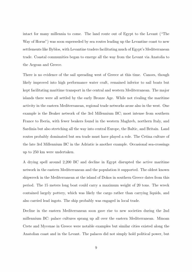
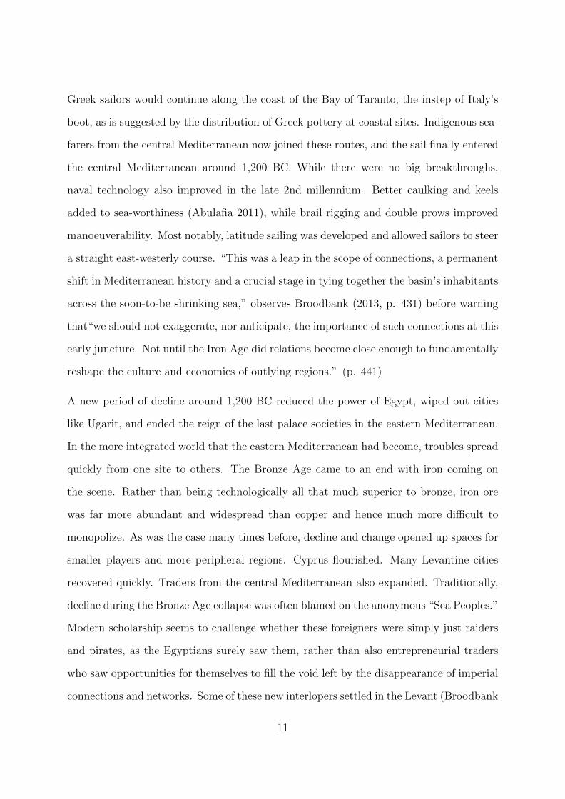
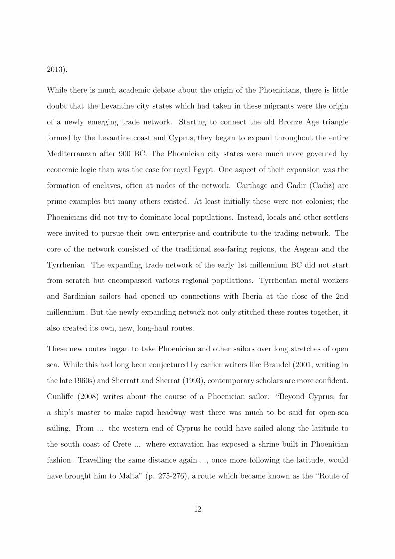
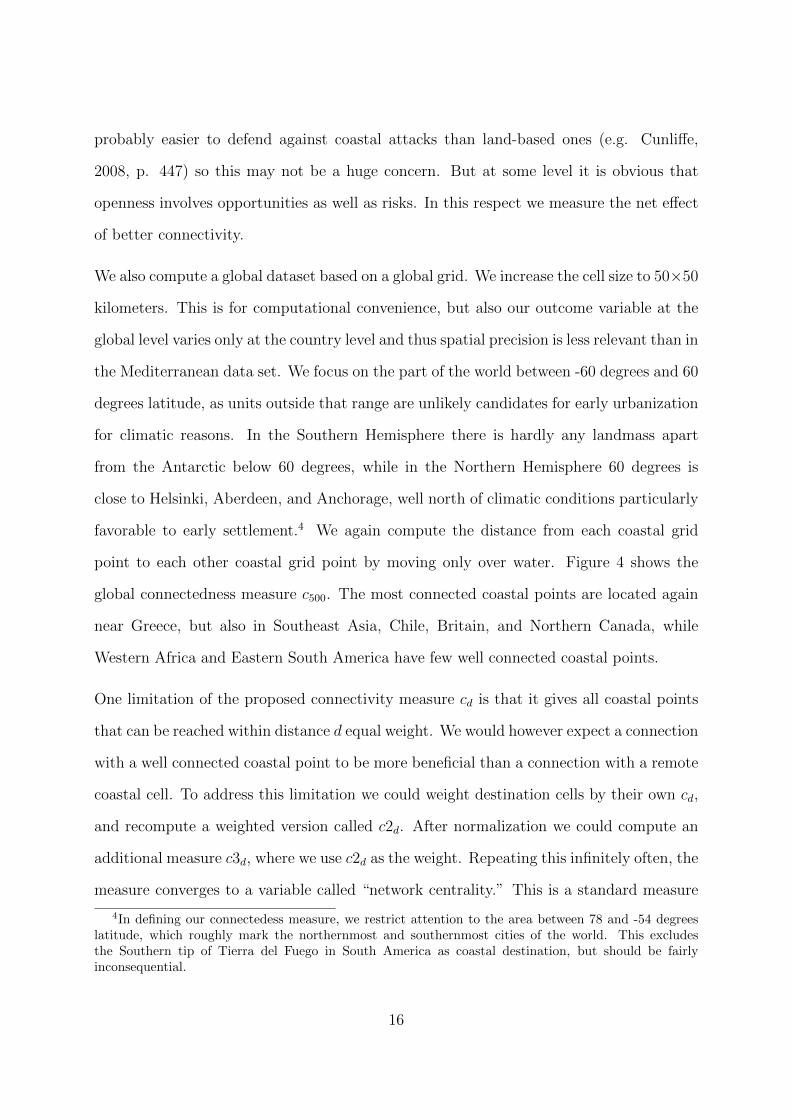
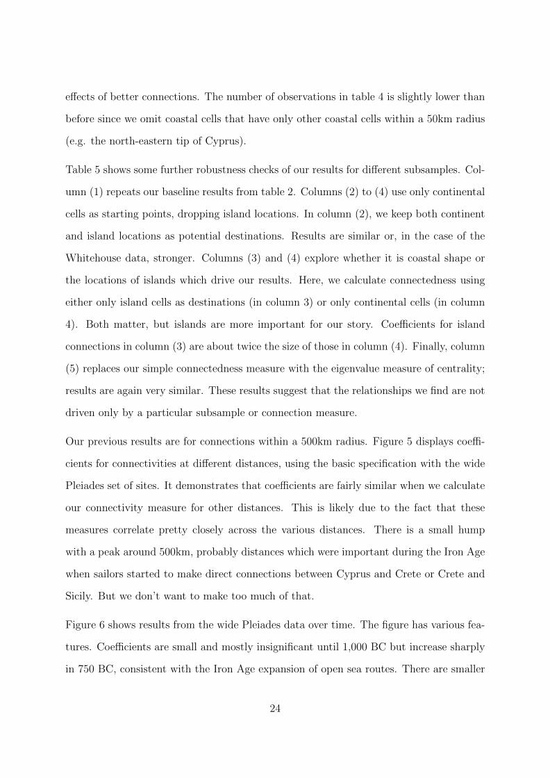
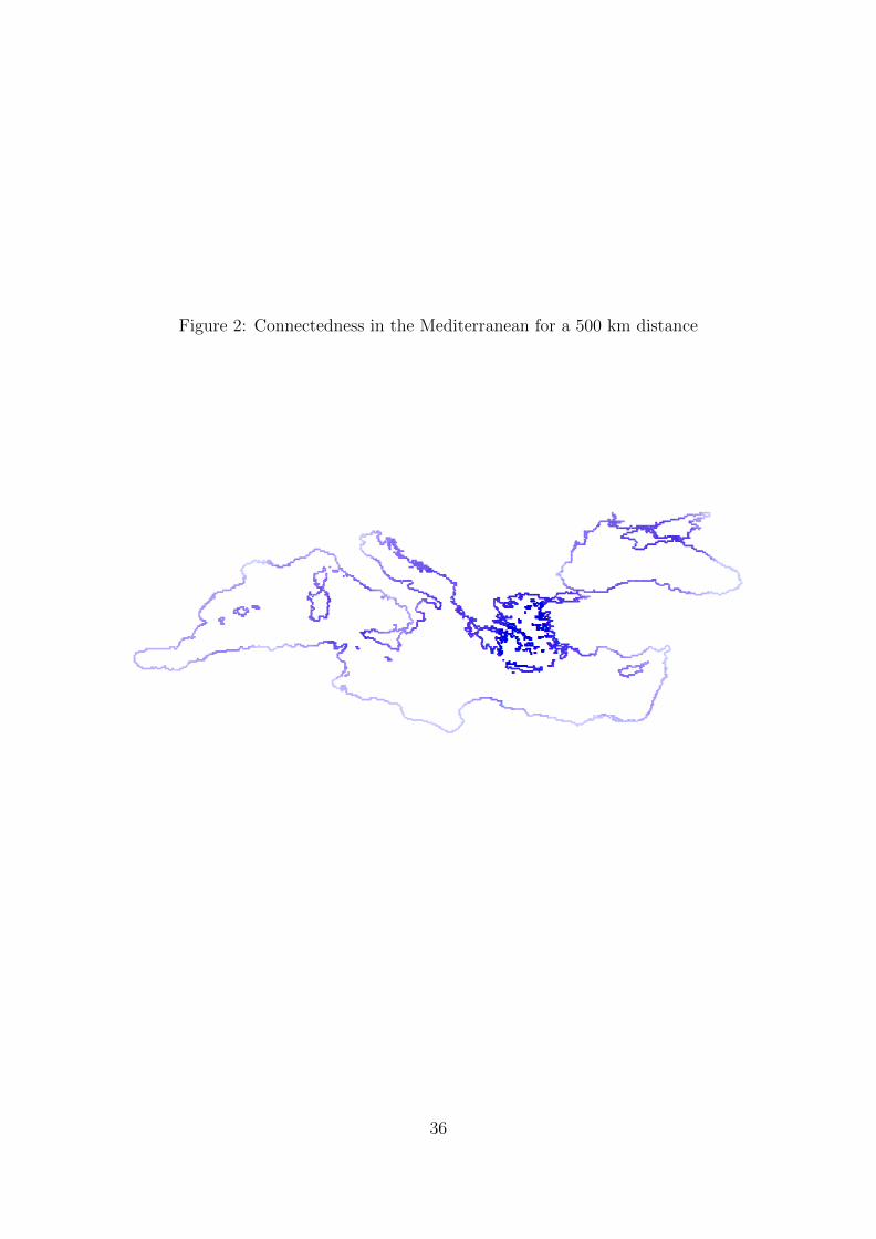
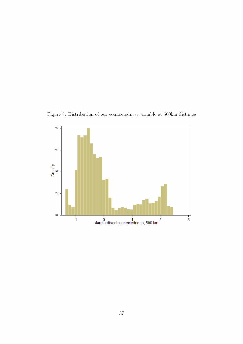
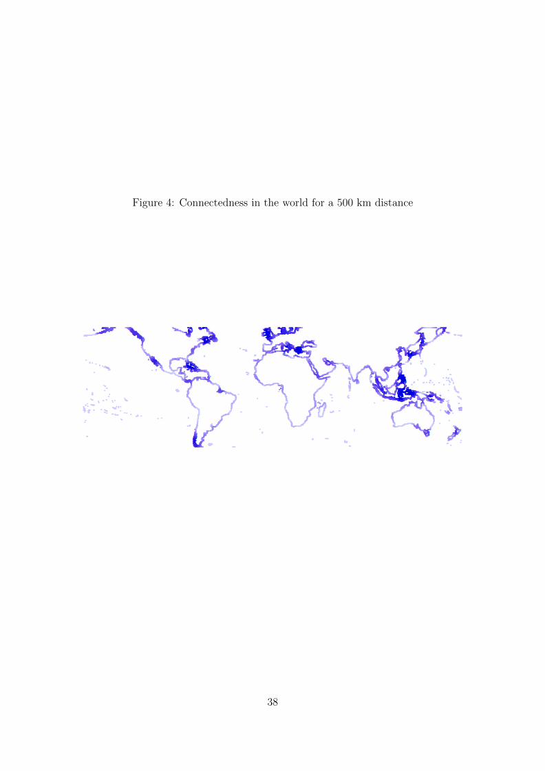
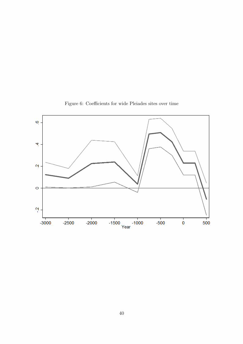
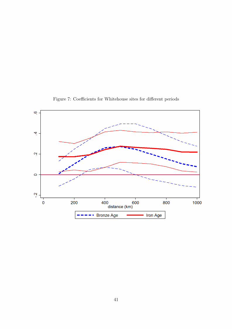
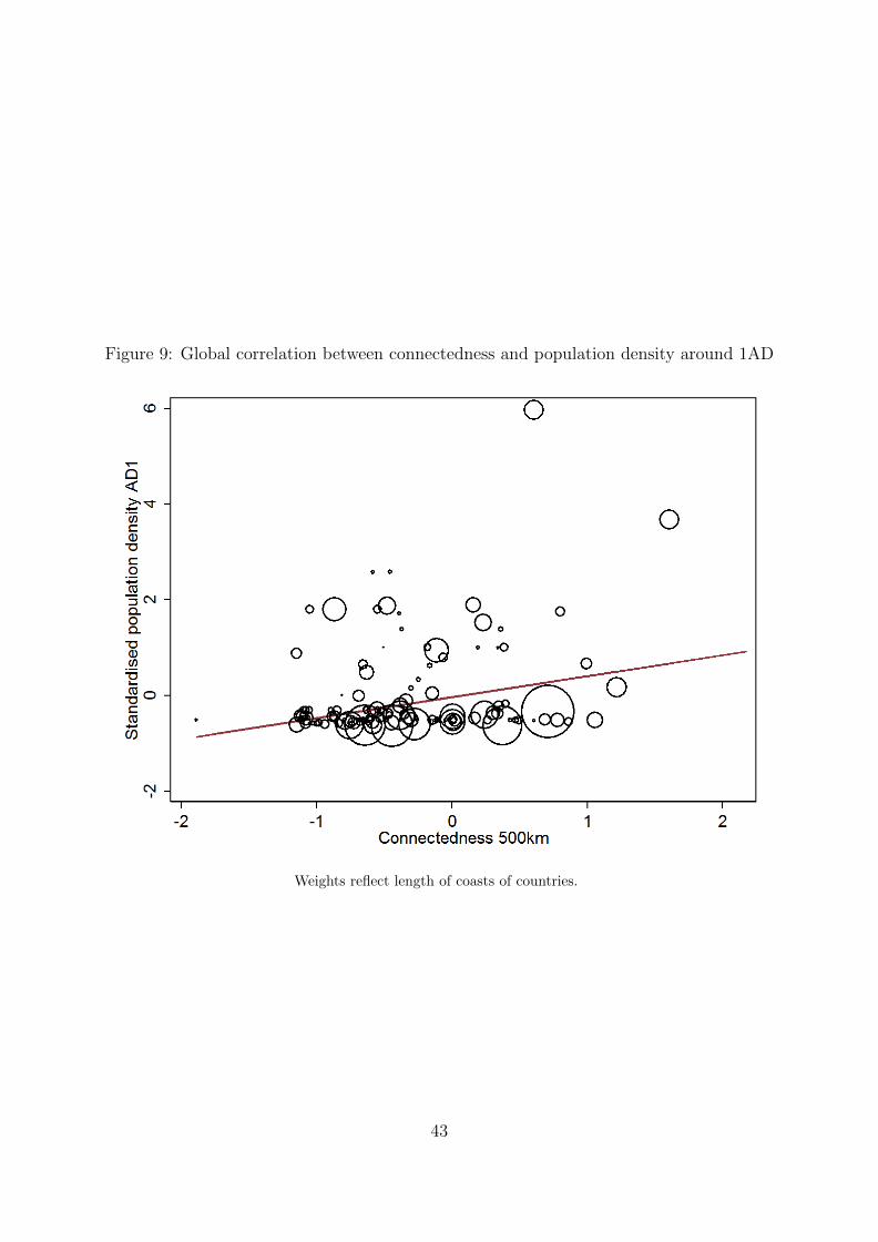
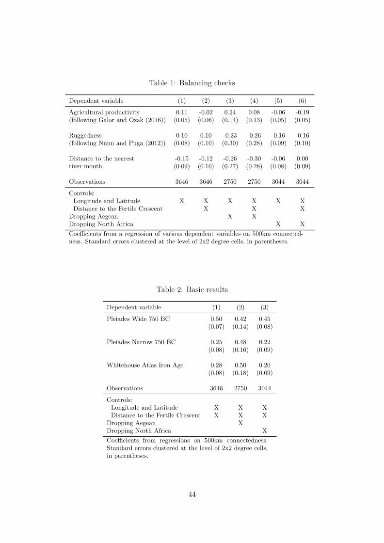
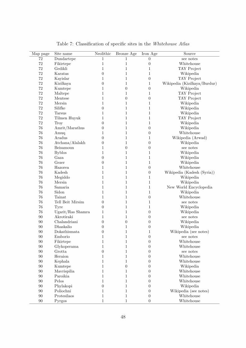
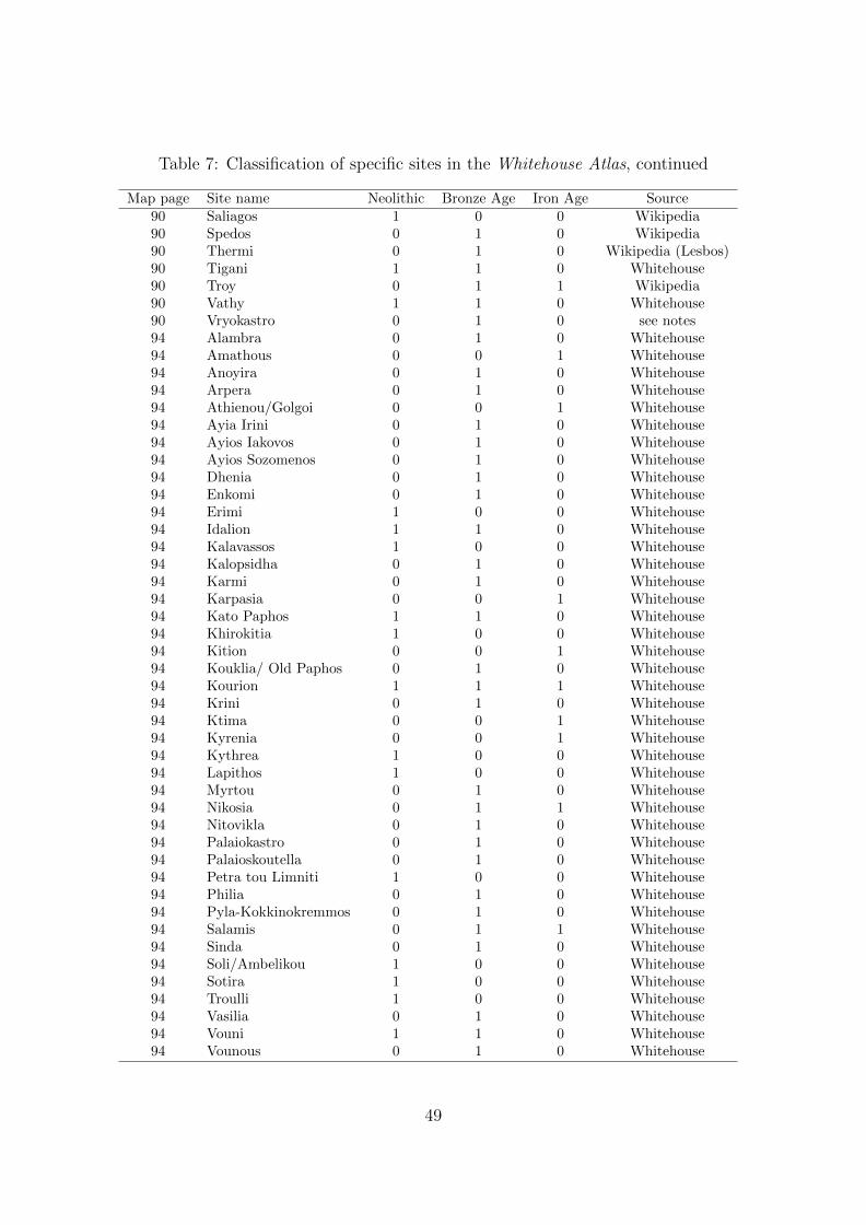
Table 7 Classification of specific sites in the Whitehouse Atlas continued
Map page Site name Neolithic Bronze Age Iron Age Source96 Amnisos 0 1 0 Wikipedia96 Apesokari 1 1 0 Wikipedia96 Apodhoulou 1 1 0 Whitehouse96 Arkhanes 0 1 0 Wikipedia96 Armenoi 1 1 0 Minoan Crete96 Ayia Triadha 0 1 1 Wikipedia (Hagia Triadna)96 Diktaean Cave 1 1 0 Wikipedia (Psychro Cave)96 Erganos 1 1 0 Whitehouse96 Fournou Korifi 0 1 0 Minoan Crete96 Gournes 1 1 0 Whitehouse96 Gournia 0 1 0 Minoan Crete96 Idaean Cave 1 1 0 Wikipedia96 Kamares Cave 1 1 0 Wikipedia96 Karfi 0 1 0 Wikipedia96 Katsamba 1 1 0 Whitehouse96 Khania 1 1 1 Wikipedia96 Knossos 1 1 1 see notes96 Krasi 1 1 0 Wikipedia (Malia Crete)96 Mallia 0 1 0 see notes96 Mirsini 1 1 0 Whitehouse96 Mirtos 1 1 0 Minoan Crete96 Mitropolis 1 1 0 Whitehouse96 Mochlos 0 1 0 Minoan Crete96 Monastiraki 0 1 0 Wikipedia96 Mouliana 1 1 0 see notes96 Palaikastro 0 1 0 Minoan Crete96 Petras 0 1 0 Wikipedia96 Phaistos 1 1 1 Wikipedia96 Pirgos (Nirou Khani) 0 1 0 Wikipedia96 Platanos 1 1 0 Whitehouse96 Plati 1 1 0 Whitehouse96 Praisos 1 1 1 Wikipedia96 Pseira 1 1 0 Wikipedia96 Rousses 1 1 0 Whitehouse96 Sklavokampos 0 1 0 Wikipedia96 Stavromenos 0 1 0 see notes96 Tylissos 0 1 0 Wikipedia96 Vasiliki 0 1 0 Wikipedia96 Vathypetro 0 1 0 Minoan Crete96 Zakro 0 1 0 Wikipedia96 Zou 1 1 0 Minoan Crete
50
Table 7 Classification of specific sites in the Whitehouse Atlas continued
Map page Site name Neolithic Bronze Age Iron Age Source102 Adana (Ataniya) 1 1 1 Wikipedia102 Al Mina 0 0 1 Wikipedia102 AmritMarathus 0 1 0 Wikipedia102 Antioch 0 0 1 Wikipedia102 Aradus 0 1 1 Wikipedia102 Askalon 1 1 1 Wikipedia102 AtchanaAlalakh 0 1 0 Wikipedia102 Atlit 0 1 1 Wikipedia102 Beersheba 1 1 1 Wikipedia102 Berytus 0 0 1 Wikipedia102 Byblos 1 1 1 Wikipedia102 Enkomi 0 1 0 Wikipedia102 Gaza 0 1 1 Wikipedia102 Hazor 0 1 1 Wikipedia102 Jaffa 1 1 1 Wikipedia102 Kadesh 1 1 0 Wikipedia102 Kourion 1 1 1 Wikipedia102 Megiddo 1 1 1 Wikipedia102 Minet el-Beida 0 1 1 see notes102 Nikosia 0 1 1 Wikipedia102 Salamis 0 1 1 Wikipedia102 Samaria 1 1 1 New World Encyclopedia102 Sarepta 0 1 1 Wikipedia102 Shechem 1 1 1 Wikipedia102 Sidon 1 1 1 Wikipedia102 Simyra 0 1 1 Wikipedia102 Tarsus 1 1 1 Wikipedia102 Tripolis 0 0 1 Wikipedia102 Tyre 0 1 1 Wikipedia102 UgaritRas Shamra 1 1 0 Wikipedia122 Bahrija 0 1 0 Whitehouse122 Borg in Nadur 0 1 0 Whitehouse122 Ghar Dalam 1 1 0 Whitehouse122 Skorba 1 0 0 Whitehouse122 Tarxien 1 1 0 Whitehouse
51
Sources and notes for site classification
Dundartepe The Cambridge Ancient History 3rd ed Vol 1 Part 2 Early History of
the Middle East eds I E S Edwards C J Gadd N G L Hammond 1971 p 400 and
Ancient West and East Vol 1 Number 2 2002 ed Gocha R Tsetskhladze p245
TAY Project httpwwwtayprojectorgveritabenghtml under the site name
Wikipedia httpsenwikipediaorg under the site name
Beisamoun Israel Antiquities Authority Beisamoun (Mallaha) httpwwwhadashot-esi
orgilreport_detail_engaspxid=809
New World Encyclopedia httpwwwnewworldencyclopediaorg under the site name
Tell Beit Mirsim Biblewalks httpwwwbiblewalkscomSitesBeitMirsimhtml
Akrotiraki httpwwwaegeanislandsgrdiscover-aigaioarchaeology-aigiao
archaeology-aigaiohtml
Dokathismata Entry under Amnorgos end date unclear but clearly settled during the
Classical period
Emborio wwwarchaeologywikiblog20160307
history-chios-seen-exhibits-archaeological-museum
Grotta httpwwwnaxosgrennaxossights-and-sightseeingarchaeological-sites
articleaid=19
Poliochni End date is unclear
Vryokastro httpwwwtinosecretgrtourmuseums512-vryokastrohtm
Minoan Crete httpwwwminoancretecomusingpull-downmenus
Knossos Wikipedia lists Knossos as abandoned around 1100 BC but the Whitehouse
Atlas has it appear again on Iron Age map 106
52
Mallia httpwwwperseustuftseduhopperartifactname=Malliaampobject=Site
Mouliana httpsmoulianaprojectorg
Stavromenos
httpsgreeceterrabookcomrethymnopagearchaelogical-site-of-stavromenos
Minet el-Beida Wikipedia No independent dating info for Minet el-Beida It is routinely
referred to as the harbor of Ugarit Hence dating the same as Ugarit
53
7 Appendix B Additional specifications
As the historical record in section 2 has shown seafaring at short distances was already
common in the Mediterranean before the Iron Age However with the advent of the
Phoenicians regular long-distance travel and trade across the open sea emerged Our
measure of 500km connectedness might conflate short-distance connectedness with long-
run one In table 8 we therefore create a different version of connectedness that is based
on points that can be reached at a distance of 100 to 500km ie excluding points within
100km The results are very similar to the basic ones in table 2
Not only connections over sea mattered but land trade was important as well Rivers
constituted important entry points for land based trade As a result cells close to river
mouths should be relatively advantaged The inland connections afforded by river mouths
might also interact with the maritime connections we have analyzed so far Sea and inland
trade maybe either complements or substitutes Table 9 investigates these possibilities
by entering a regressor for distance to the nearest river mouth in our regressions and
interacting it with our sea based connectivity measure The main effect of the connected-
ness variable is affected little by these additions The main effect for distance to a river
mouth is positive indicating that locations close to a river mouth have fewer settlements
not more But the coefficients are small and not significant The interaction terms are
similarly small except in the specification without the Aegean where we find a positive
(but at most marginally significant) interaction effect This would suggest that coastal
and inland connections are substitutes rather than complements
54
Table 8 Results when excluding short-distance connectedness
Dependent variable (1) (2) (3)
Pleiades Wide 750 BC 050 043 045(007) (013) (008)
Pleiades Narrow 750 BC 026 051 022(008) (015) (009)
Whitehouse Atlas Iron Age 027 052 019(008) (017) (009)
Observations 3646 2750 3044
ControlsLongitude and Latitude X X XDistance to the Fertile Crescent X X X
Dropping Aegean XDropping North Africa X
Coefficients from regressions on connectedness be-tween 100 and 500km Standard errors clustered atthe level of 2x2 degree cells in parentheses
Table 9 Results with interactions
Regressor (1) (2) (3)
Connectedness 049 043 045(007) (014) (008)
Distance to 008 017 007river mouth (006) (013) (009)
Interaction 009 019 002(005) (011) (007)
Observations 3646 2750 3044
ControlsLongitudeLatitude X X XDistance to the Fertile Crescent X X X
Dropping Aegean XDropping North Africa X
Pleiades wide data Coefficients from regressions on
500km connectedness Standard errors clustered at the
level of 2x2 degree cells in parentheses
55
- Introduction
- Brief history of ancient seafaring in the Mediterranean
- Data and key variables
- Specification and results
-
- Basic results
- Persistence
- Results for a world scale
-
- Conclusion
- Appendix A Coding of Whitehouse sites
- Appendix B Additional specifications
-
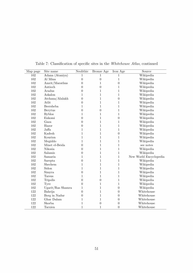
Table 7 Classification of specific sites in the Whitehouse Atlas continued
Map page Site name Neolithic Bronze Age Iron Age Source102 Adana (Ataniya) 1 1 1 Wikipedia102 Al Mina 0 0 1 Wikipedia102 AmritMarathus 0 1 0 Wikipedia102 Antioch 0 0 1 Wikipedia102 Aradus 0 1 1 Wikipedia102 Askalon 1 1 1 Wikipedia102 AtchanaAlalakh 0 1 0 Wikipedia102 Atlit 0 1 1 Wikipedia102 Beersheba 1 1 1 Wikipedia102 Berytus 0 0 1 Wikipedia102 Byblos 1 1 1 Wikipedia102 Enkomi 0 1 0 Wikipedia102 Gaza 0 1 1 Wikipedia102 Hazor 0 1 1 Wikipedia102 Jaffa 1 1 1 Wikipedia102 Kadesh 1 1 0 Wikipedia102 Kourion 1 1 1 Wikipedia102 Megiddo 1 1 1 Wikipedia102 Minet el-Beida 0 1 1 see notes102 Nikosia 0 1 1 Wikipedia102 Salamis 0 1 1 Wikipedia102 Samaria 1 1 1 New World Encyclopedia102 Sarepta 0 1 1 Wikipedia102 Shechem 1 1 1 Wikipedia102 Sidon 1 1 1 Wikipedia102 Simyra 0 1 1 Wikipedia102 Tarsus 1 1 1 Wikipedia102 Tripolis 0 0 1 Wikipedia102 Tyre 0 1 1 Wikipedia102 UgaritRas Shamra 1 1 0 Wikipedia122 Bahrija 0 1 0 Whitehouse122 Borg in Nadur 0 1 0 Whitehouse122 Ghar Dalam 1 1 0 Whitehouse122 Skorba 1 0 0 Whitehouse122 Tarxien 1 1 0 Whitehouse
51
Sources and notes for site classification
Dundartepe The Cambridge Ancient History 3rd ed Vol 1 Part 2 Early History of
the Middle East eds I E S Edwards C J Gadd N G L Hammond 1971 p 400 and
Ancient West and East Vol 1 Number 2 2002 ed Gocha R Tsetskhladze p245
TAY Project httpwwwtayprojectorgveritabenghtml under the site name
Wikipedia httpsenwikipediaorg under the site name
Beisamoun Israel Antiquities Authority Beisamoun (Mallaha) httpwwwhadashot-esi
orgilreport_detail_engaspxid=809
New World Encyclopedia httpwwwnewworldencyclopediaorg under the site name
Tell Beit Mirsim Biblewalks httpwwwbiblewalkscomSitesBeitMirsimhtml
Akrotiraki httpwwwaegeanislandsgrdiscover-aigaioarchaeology-aigiao
archaeology-aigaiohtml
Dokathismata Entry under Amnorgos end date unclear but clearly settled during the
Classical period
Emborio wwwarchaeologywikiblog20160307
history-chios-seen-exhibits-archaeological-museum
Grotta httpwwwnaxosgrennaxossights-and-sightseeingarchaeological-sites
articleaid=19
Poliochni End date is unclear
Vryokastro httpwwwtinosecretgrtourmuseums512-vryokastrohtm
Minoan Crete httpwwwminoancretecomusingpull-downmenus
Knossos Wikipedia lists Knossos as abandoned around 1100 BC but the Whitehouse
Atlas has it appear again on Iron Age map 106
52
Mallia httpwwwperseustuftseduhopperartifactname=Malliaampobject=Site
Mouliana httpsmoulianaprojectorg
Stavromenos
httpsgreeceterrabookcomrethymnopagearchaelogical-site-of-stavromenos
Minet el-Beida Wikipedia No independent dating info for Minet el-Beida It is routinely
referred to as the harbor of Ugarit Hence dating the same as Ugarit
53
7 Appendix B Additional specifications
As the historical record in section 2 has shown seafaring at short distances was already
common in the Mediterranean before the Iron Age However with the advent of the
Phoenicians regular long-distance travel and trade across the open sea emerged Our
measure of 500km connectedness might conflate short-distance connectedness with long-
run one In table 8 we therefore create a different version of connectedness that is based
on points that can be reached at a distance of 100 to 500km ie excluding points within
100km The results are very similar to the basic ones in table 2
Not only connections over sea mattered but land trade was important as well Rivers
constituted important entry points for land based trade As a result cells close to river
mouths should be relatively advantaged The inland connections afforded by river mouths
might also interact with the maritime connections we have analyzed so far Sea and inland
trade maybe either complements or substitutes Table 9 investigates these possibilities
by entering a regressor for distance to the nearest river mouth in our regressions and
interacting it with our sea based connectivity measure The main effect of the connected-
ness variable is affected little by these additions The main effect for distance to a river
mouth is positive indicating that locations close to a river mouth have fewer settlements
not more But the coefficients are small and not significant The interaction terms are
similarly small except in the specification without the Aegean where we find a positive
(but at most marginally significant) interaction effect This would suggest that coastal
and inland connections are substitutes rather than complements
54
Table 8 Results when excluding short-distance connectedness
Dependent variable (1) (2) (3)
Pleiades Wide 750 BC 050 043 045(007) (013) (008)
Pleiades Narrow 750 BC 026 051 022(008) (015) (009)
Whitehouse Atlas Iron Age 027 052 019(008) (017) (009)
Observations 3646 2750 3044
ControlsLongitude and Latitude X X XDistance to the Fertile Crescent X X X
Dropping Aegean XDropping North Africa X
Coefficients from regressions on connectedness be-tween 100 and 500km Standard errors clustered atthe level of 2x2 degree cells in parentheses
Table 9 Results with interactions
Regressor (1) (2) (3)
Connectedness 049 043 045(007) (014) (008)
Distance to 008 017 007river mouth (006) (013) (009)
Interaction 009 019 002(005) (011) (007)
Observations 3646 2750 3044
ControlsLongitudeLatitude X X XDistance to the Fertile Crescent X X X
Dropping Aegean XDropping North Africa X
Pleiades wide data Coefficients from regressions on
500km connectedness Standard errors clustered at the
level of 2x2 degree cells in parentheses
55
- Introduction
- Brief history of ancient seafaring in the Mediterranean
- Data and key variables
- Specification and results
-
- Basic results
- Persistence
- Results for a world scale
-
- Conclusion
- Appendix A Coding of Whitehouse sites
- Appendix B Additional specifications
-
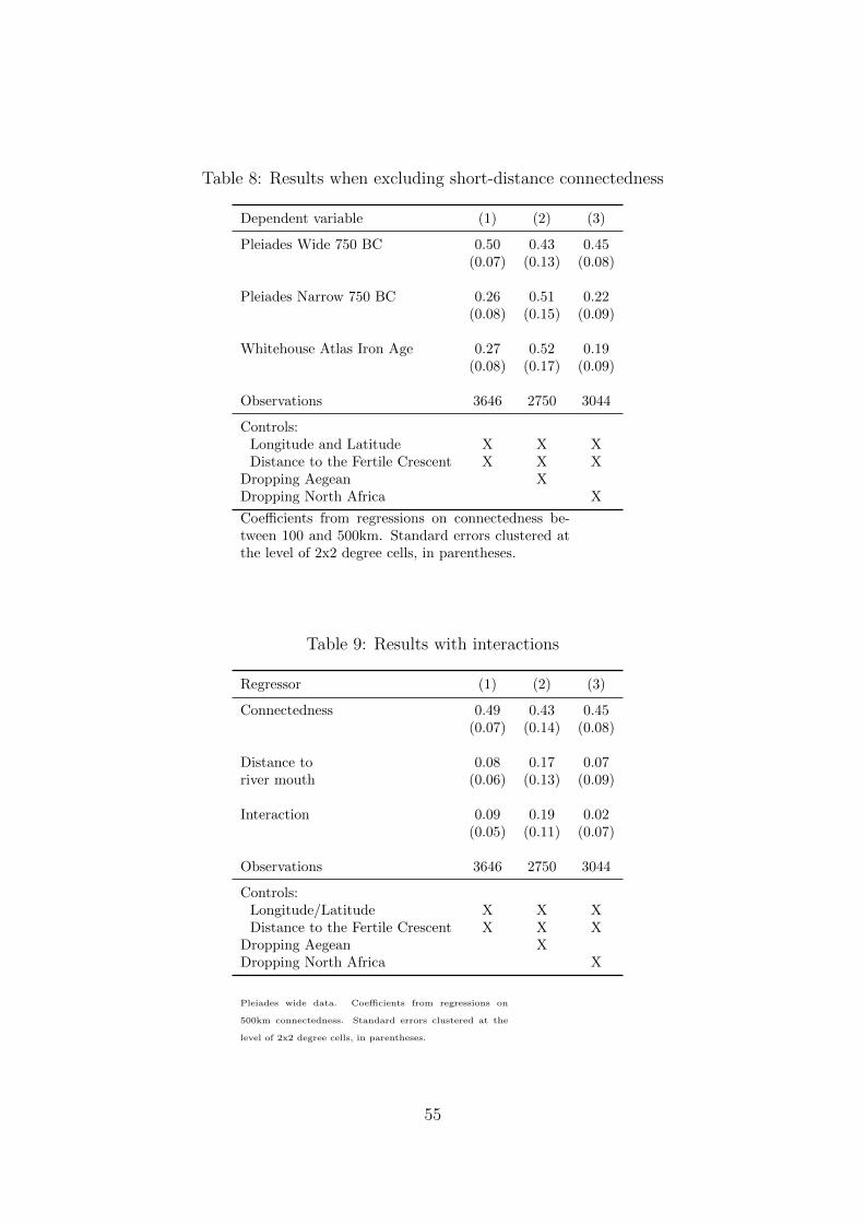


![Role of alcohol in the regulation of iron metabolism · iron metabolism. Hepcidin knockout mice develop iron overload in the liver, pancreas and heart[58], whereas mice overexpressing](https://static.fdocuments.us/doc/165x107/5f59a9c0466a1b6ca069718a/role-of-alcohol-in-the-regulation-of-iron-metabolism-iron-metabolism-hepcidin-knockout.jpg)