of Langmuir waves in the linear regime

MNRAS 000, 1–21 (2015) Preprint 31 July 2020 Compiled using MNRAS LATEX style file v3.0

Pulsar radio emission mechanism I : On the amplificationof Langmuir waves in the linear regime

Sk. Minhajur Rahaman,1? Dipanjan Mitra,1,2 George I. Melikidze2,31,National Centre for Radio Astrophysics,Tata Institute of Fundamental Research, Post Bag 3, Ganeshkind,Pune-411007,INDIA2Janusz Gil Institute of Astronomy, University of Zielona Gora, ul Szafrana 2, 65-516 Zielana Gora, Poland3 Evgeni Kharadze Georgian National Astrophysical Observatory, 0301, Abastumani, Georgia

Accepted XXX. Received YYY; in original form ZZZ

ABSTRACTObservations suggest that in normal period radio pulsars, coherent curvature radiationis excited within 10% of the light cylinder. The coherence is attributed to Langmuirmode instability in a relativistically streaming one-dimensional plasma flow along theopen magnetic field lines. In this work, we use a hot plasma treatment to solve the hy-drodynamic dispersion relation of Langmuir mode for realistic pulsar parameters. Thesolution involves three scenarios of two-stream instability viz., driven by high energybeams, due to longitudinal drift that leads to a separation of electron-positron distri-bution functions in the secondary plasma and due to cloud-cloud interaction causingspatial overlap of two successive secondary plasma clouds. We find that sufficient am-plification can be obtained only for the latter two scenarios. Our analysis shows thatlongitudinal drift is characterized by high growth rates only for certain multi-polarsurface field geometry. For these configurations, very high growth rates are obtainedstarting from a few tens of km from the neutron star surface, which then falls mono-tonically with increasing distance. For cloud-cloud overlap, growth rates become highstarting only after a few hundred km from the surface, which first increases and thendecreases with increasing distance. A spatial window of up to around a 1000 km abovethe neutron star surface has been found where large amplitude Langmuir waves canbe excited while the pair plasma is dense enough to account for high brightness tem-perature.

Key words: pulsars – radiation mechanism – relativistic plasma – Langmuir mode

1 INTRODUCTION

Observations of radio emission from normal period pulsars(with periods P longer than ∼ 0.1 seconds) suggest that:a) The radio emission has exceedingly high brightness tem-perature Tb ∼ 1025 − 1027 K, which is at least 12 orders ofmagnitude higher than the incoherent synchrotron limit of1012 K (see Kellermann & Pauliny-Toth 1969 ). This nec-essarily requires a coherent radio emission mechanism (e.g.Ginzburg et al. 1969; Ginzburg & Zhelezniakov 1975; Cordes1979; Melrose 1993; Mitra 2017) ; b) The radio emission ishighly polarized, which is consistent with coherent curvatureradiation ( hereafter CCR ) (e.g. Mitra et al. 2009; Melikidzeet al. 2014) ; c) The radio emission detaches from the pul-sar magnetosphere a few hundred km away from the surface(e.g. Rankin 1993; Mitra 2017).

? E-mail: [email protected]

These observations require plasma processes where sta-ble charge bunches can form and excite CCR in relativis-tically streaming pair plasma, which can eventually escapefrom the plasma to reach the observer (see Melikidze et al.2014; Gil et al. 2004; Mitra et al. 2009). For a general non-zero angle between the propagation vector and the ambientmagnetic field, the pulsar pair plasma consists of two eigen-modes viz., the purely transverse X-mode and the quasi-transverse O-mode (see Arons & Barnard 1986). The quasi-transverse O-mode has a sub-Lumininal Alfven branch andsuper-Luminal LO branch. A number of works show thatcyclotron instabilities of the X and O modes can be excitedclose to the light-cylinder (see for e.g. Kazbegi et al. 1991;Lyutikov 1999). However, several works have shown thatclose to neutron star surface, where the radio emission orig-inates, the excitation of the Alfven branch is inefficient(e.g.Lominadze et al. 1986; Kazbegi et al. 1991 ; Lyutikov 2000).For the special case when the angle between the propagationvector and the ambient magnetic field is zero, the O-modebecomes purely longitudinal and is referred to as the Lang-

© 2015 The Authors

arX

iv:2

007.

1539

5v1

[as

tro-

ph.H

E]

30

Jul 2

020

2 Rahaman et al.

muir mode (see fig. 2 of Arons & Barnard 1986). It has beenshown in several studies (e.g. Usov 2002) that closer to theneutron star surface this longitudional Langmuir mode canbecome unstable. Langmuir mode instability is a popularcandidate for these CCR charge bunches. Theoretically, acombination of linear and non-linear plasma theory is neededto form stable charge bunch (see Melikidze et al. 2000). Thelinear part of the theory involves development of two streaminstability in the plasma that leads to the growth of the am-plitude of the longitudinal and electrostatic Langmuir wavemode. While the oscillating electric field of the Langmuirmode can form longitudinal concentrations of charges, itis well known that such linear Langmuir bunches are notcapable of radiating coherently (see e.g. Lominadze et al.1986; Melikidze et al. 2000). Analytical studies show thatunder certain approximations stable bunches viz. relativis-tic Langmuir charge soliton can form when non-linear ef-fects are taken into account (see Pataraia & Melikidze 1980;Melikidze et al. 2000). Recent numerical analysis have alsofound such stable charge bunches, when all non-linear inter-actions are properly taken into account (see Lakoba et al.2018). However there are several gaps in the theory thatremains to be addressed. The non-linear theory requires apriori very large amplitude for the electrostatic waves. Thecrucial question of quantitative estimates of linear growthrates of Langmuir waves for realistic pulsar plasma parame-ters, and if the growth rate is sufficient to drive the systembeyond the linear regime requires thorough investigation.

The radio emission is excited in relativistically stream-ing pulsar plasma that consists of a dense secondarypositron-electron (e+e−) pair plasma, a tenuous high en-ergy primary positron or electron (e+/e−) beam and a ten-uous high energy ion beam. The growth of Langmuir insta-bility requires a two-stream condition to be established inthis plasma. Some early works on Langmuir mode in pulsarplasma in fact concluded that Langmuir mode cannot be-come unstable (e.g. Suvorov & Chugunov 1975 ). HoweverLominadze & Mikhailovskii (1979), discussed that in rela-tivistic plasma, particles close to the velocity of light canbe in resonance with the Langmuir mode. The authors alsodiscussed two regimes of growth viz., the kinetic and thehydrodynamic regime. There are three ways (referred to ascase C1, C2, C3 hereafter) by which the two-stream insta-bility can develop in this flow: first for C1 between the highenergy beams and secondary plasma system, second for C2between the electrons and positrons in the secondary plasmaitself due to longitudinal drift, and third for C3 between theoverlapping fast and slow particles overlap of successive sec-ondary plasma clouds due to intermittent discharges at thepolar gap.

Previous studies of the growth of Langmuir wave in pul-sar plasma for the three aforementioned cases of two-streaminstability can be briefly summarized as follows:

C1: Initial studies of pulsar radio emission mechanism (e.g.Ruderman & Sutherland 1975 hereafter RS75) appealed toa two-stream instability driven by high energy cold e+/e−beam. Subsequent works(e.g. Benford & Buschauer 1977)found very small growth rates for such e+/e− cold beam.Egorenkov et al. (1983) presented a hot plasma treatment of

the high energy e+/e− beam and showed that kinetic regimeis suppressed and only the hydrodynamic regime survives.Gedalin et al. (2002) explored beam-driven hydrodynamicinstability of a low frequency longitudinal beam mode ratherthan the high-frequency Langmuir mode. Most of the sub-sequent works (see Lyutikov 1999; Melrose & Gedalin 1999;Rafat et al. 2019) have focussed on this e+/e− beam andfound the growth rates to be negligible.

C2: The study by Cheng & Ruderman (1977, hereafterCR77) showed that as the secondary pair plasma movesalong the curved magnetic field line, longitudinal drift causesthe electron and positron distribution function to separate.This can lead to two-stream instability in the secondaryplasma. However, they did not consider a hot plasma treat-ment of the secondary plasma and obtained order of mag-nitude estimates of growth rate using simple assumptions.Asseo & Melikidze (1998, hereafter AM98) revisited theproblem where they presented a hot plasma treatment ofthe shifted electron-positron distribution function within thesecondary plasma cloud.

C3: Usov (1987) showed that in non-stationary plasma flowmodels, slow and fast moving particles of two successiveplasma clouds can overlap within a few hundred km fromthe surface leading to the development of a two-stream in-stability in the overlapping region. Ursov & Usov (1988)revisited the problem and tried to estimate growth rates byapproximating the distribution function of the fast and slowparticles in the overlapping region by delta-function. AM98extended and presented a more realistic analytical way ofconstructing the form of the hot plasma distribution func-tion in the overlapping region.

The aforementioned studies suggest that large ampli-tude Langmuir wave cannot exist due to e+/e− beam in C1.AM98 showed that two-stream instability in C2 and C3 canresult in high growth rates of Langmuir wave. They alsofound that the growth rate for C3 to be significantly largerthan C2. Thus AM98 provided the necessary justification,that in principle large amplitude Langmuir waves can betriggered for both C2 and C3.

However AM98 obtained growth rates in the hydrody-namic regime for C2 and C3 using many simplifying assump-tions. For example, they assumed the surface magnetic fieldto be dipolar while observations suggest the existence of astrong multipolar magnetic field at the surface. Also, theyestimated growth rates as a function of the distance fromthe neutron star, using coarse spatial ( and temporal ) reso-lution. In their numerical scheme, AM98 did not obtain thecomplete solution of the dispersion relation at a given heightand estimated growth rates only for some representativewave numbers. The coarse resolution in their analysis canwash away many important features of the evolution of thegrowth rate as a function of the distance from the neutronstar. Hence it is necessary to undertake an updated studyof AM98 where these shortcomings should be addressed ap-propriately. This is the primary focus of this work. Furtherkeeping in view that a tenous high energy beam of ions canexist, we study the effect of the same on Langmuir modeinstability in C1 and compare it with the e+/e− beam.

MNRAS 000, 1–21 (2015)

Linear amplification of Langmuir waves 3

It must be noted that the amplification of the Langmuirwave for a given frequency ω depends on the gain ‘G’ whichis a product of the growth rate (ωI) and the time availablefor growth (∆t) as the amplitude is ∝ eG=ωI∆t . If time ∆t issmall, even with a high ωI, the amplification factor G will besmall and one cannot use these waves to participate in thecoherent emission mechanism. In this work, we go beyondjust the estimation of growth rate and present a methodthat employs the complete bandwidth of the growing wavesto estimate ∆t and thereby the maximum gain possible fora given frequency. We present an exhaustive treatment ofLangmuir mode instability for C1, C2 and C3 to examinethe existence of large amplitude Langmuir waves in the pul-sar radio emission region. The outline of the paper is asfollows: In sections 2 we discuss physical constraints for thehot plasma description and models of plasma flow. In sec-tions 3 and 4 we describe the analysis method for the linearLangmuir instability and study the growth rates and gainfactors for these cases. In sections 5 and 6 we discuss theresults and state our conclusions.

2 INPUTS TO THE PULSAR PLASMAPARAMETERS

2.1 Constraints from radio emission height

A number of studies : Blaskiewicz et al. (1991), von Hoens-broech & Xilouris (1997) , Mitra & Li (2004) , Mitra &Rankin (2011) , Weltevrede & Johnston (2008) has consis-tently found the emission region to be below 10 % of LCacross pulsar period (see fig. 3 of Mitra 2017). As discussedby Mitra & Li (2004), the various methods employed to findradio emission heights can be affected due to measurementas well as systematic errors, however for normal pulsars av-erage estimates of a few hundred kilometers above the neu-tron star surface is considered reasonable. Specific studies(e.g. Mitra & Rankin 2002) also, focus on estimating therange of emission heights as a function of frequency, and itis found that a certain radius to frequency mapping existsin pulsars where progressively higher frequencies arise closerand closer to the neutron star surface. These studies revealthat the broad-band pulsar emission range from about fewten to hundred km at the highest frequency ∼ 5 GHz andto several hundred km at the lowest frequency ∼ 100 MHz.Kazbegi et al. (1991) showed that cyclotron resonances canbe excited only near the light cylinder. At the radio emissionheights all cyclotron resonances are suppressed and only theCherenkov resonance condition can operate.

2.2 Signature of Coherent Curvature Radiation

Several lines of evidence (see Lai et al. 2001; Johnston et al.2005; Rankin 2007; Noutsos et al. 2012, 2013; Force et al.2015) have revealed that the polarization of the emergentpulsar radiation are directed either perpendicular or paral-lel to the magnetic field line plane. These polarization modesare commonly referred to as the extraordinary and Ordinary

mode respectively which are defined with their electric fieldvector being perpendicular and parallel to the magnetic fieldplane respectively. The eigenmodes of the pulsar plasma viz.,the X-mode and the O-mode is perpendicular and parallelto the ®k − ®B plane, where ®B is the ambient magnetic fieldand ®k is the propagation vector of the wave. If the under-lying excitation mechanism is due to CCR, then these twoplanes need to be co-incident. For any other form of excita-tion, these two planes can maintain arbitrary orientation toeach other. This implies that the polarization of emergent ra-diation carries information about the underlying excitationmechanism. This idea was applied by Mitra et al. (2009) to asample of nearly 100 % linearly polarized single pulses whichestablished CCR as the underlying emission mechanism.

2.3 Multi-polar surface magnetic fields andparticle flows

It is well known (see e.g. Mitra & Li 2004) that at a few hun-dred kilometers above the neutron star surface, from regionswhere the radio emission originates, the underlying magneticfield structure is dipolar. However, in recent years there areseveral pieces of evidence for the presence of surface multi-polar fields. For example Gil & Mitra (2001) and Mitra et al.(2020) suggested that the radio-loud nature of the extremallong period 8.5 s pulsar J2144-3933 (Young et al. 1999) canonly be explained if surface magnetic fields have a radius ofcurvature ρc ∼ 105 cm at the surface, which is only possibledue to presence of strong multipolar surface magnetic field.The X-ray observations have also confirmed the presence ofmultipolar fields on the surface (see e.g. Arumugasamy &Mitra 2019).

The presence of multipolar surface magnetic field signif-icantly affects the description of the plasma. At the polar capmagnetically induced pair creation processes are triggered.The presence of multipolar surface magnetic field decreasesthe radius of curvature at the surface thereby increasing theefficiency of the pair creation process. As a result the num-ber density of the pair plasma exceeds the co-rotational valuenGJ by a multiplicity factor κGJ. Observations of PWNe hasrevealed κGJ ∼ 104 − 105 (see de Jager 2007 ; Blasi & Amato2011 ). To get this high value of κGJ estimations show that toget κGJ ∼ 104−105 multi-polar fields are required (see Medin& Lai 2010 ; Szary et al. 2015 ; Timokhin & Harding 2019)whereas for purely dipolar fields κGJ is about the order of afew tens to hundred (see Hibschman & Arons 2001; Arendt& Eilek 2002)

2.3.1 Need for multipolar surface magnetic field for CCR

The limiting brightness temperature for incoherent cur-vature radiation is T ICR

lim ≈ 1013 K (see Melrose 1978).In the Rayleigh-Jeans regime, the brightness temperatureis proportional to power. CCR is an ‘N2’ process mean-ing if ‘N’ particles are involved, the power is boosted bya factor ‘N’ compared to what would be achieved if the

MNRAS 000, 1–21 (2015)

4 Rahaman et al.

charged particles were emitting independently (or incoher-ently). The number of particles participating in CCR to ex-plain the observed high brightness temperature is given byNCCR = Tobs/T ICR

lim ≈ 1012. Radio emission from pulsarsare received from 10 MHz to 10 GHz. The length of thebunch should satisfy the constraint L c/νHigh ∼ 3 cmfor coherence to be maintained for all frequencies. Assum-ing L ∼ 1 cm, the corresponding number density requirednCCR ∼ 1012 cm−3. At an emission height of rem = 50 RNS,the Goldreich-Julian value is given by nGJ = 5.52 ×108 (1 sec / P) (B / 1012 Gauss) (rNS/rem)3 cm−3 (see Goldre-ich & Julian 1969). Thus, CCR requires number density inexcess of the Goldreich-Julian value by a factor of 104.

2.3.2 Description of particle flow and secondary plasmadistribution functions

The models of plasma flow can be divided into two classes: a)The steady flow model (also known as SCLF model) given byArons & Scharlemann (1979) where when condition above

the polar cap is such that ®ΩRot · ®B > 0 (here ®ΩRot = 2π/P isthe pulsar rotational frequency), the electrons can be eas-ily pulled out from the star and a stationary flow of electronbeam-plasma can be maintained and; b) The non-stationaryspark discharge model (also referred to Inner accelerationgap model or the pure vacuum gap model) by RS75 for pul-

sars with ®ΩRot · ®B < 0 giving rise to an intermittent plasmaflow due to sparking discharges at the polar gap. In boththese models the beam-plasma system is established.

The vacuum gap model of RS75 is more successful inexplaining pulsar radio observations like sub-pulse drift phe-nomenon, however the original model required certain mod-ifications. Gil et al. (2003) noticed that the sub-pulse driftrates and the temperature of the thermal X-ray emittingpolar cap are both lower than that predicted by the purevacuum gap model of RS75. They suggested that the purevacuum gap is untenable and must be partially screenedsuch that the potential is ∆Vvac across the gap is replacedby η ∆Vvac where η is the screening factor. For a pulsarof period 1 second and dipolar magnetic strength of 1012

gauss, the maximum potential drop available in vacuum is∆Vvac = 6 × 1012 volts. The authors constrained η = 0.1 ,which gives the Lorentz factor of the high energy primarybeams of e+/e− and ions to be given by γb,e+/e− ∼ 106 and

γb,ions ∼ 103 respectively. Assuming CCR we can find anorder of magnitude estimate of the bulk Lorentz factor ofthe secondary pair plasma. Most of the power in CCR forcharge bunch with Lorentz factor γ is concentrated near thecritical frequency ωc = 1.5 γ3c / ρc, (see Jackson 1962,where c is the velocity of light). Assuming observing fre-quency νobs = 1.4 GHz to be close to the critical frequencyat rem = 50 RNS where ρc ≈ 108 cm, we have γ ≈ 200−300.

For our work we assume the distribution functions ofall the species to be relativistically streaming gaussians. Forsecondary plasma, the mean and the width are assumed tobe ∼ 200− 300 and ∼ 40− 60 respectively. Note that the twostream-condition can be established in non-stationary flow

by all three cases of C1, C2 and C3 whereas for stationaryflow only the cases C1 and C2.

To summarize CCR needs to be excited by large am-plitude Langmuir waves in a hot relativistically streamingdense secondary pair plasma . At the radio emission heights,the wave-particle interaction is mediated by the Cherenkovresonance condition. In subsequent sections we address howlarge amplitude Langmuir waves can be triggered for thethree cases, C1,C2, C3 of two-stream instability discussedearlier.

3 ANALYSIS OF LANGMUIR INSTABILITY

In the following subsections, we establish the methodologyfor studying Langmuir instability. To do this we define athreshold gain for a wave of a particular frequency that canbe used as a proxy for the breakdown of the linear theory.This, in turn, is achieved by solving the complex frequenciesusing the appropriate dispersion relation. For this analysis,the following aspects need to be considered.

3.1 The Dispersion relation in the observer frameof reference

The dispersion relation of the Langmuir mode for a strictlyone-dimensional relativistic flow in the observer frame of ref-erence is given by (see section 4 of AM98)

ε(ω, k) = kc +∑α ω

2p,α

∫ +∞−∞ dpα

∂ f(0)α

∂pα1

(ω−βα kc) = 0 (1)

where ω2p,α = 4πnαq2

α/mα; γ =√

1 + p2α; βα = pα/

√1 + p2

α.

Here nα, qα, mα, pα and f (0)α is the number density, charge,mass, dimensionless momenta and the equilibrium distribu-tion function of the α-th species in the plasma such that

nα = κGJ,α nGJ, pα = γmαv/mαc = γβ and∫ +∞−∞ dpα f (0)α = 1.

We assume f (0)α = (1/(√

2πσ2α) exp [−(pα − µα)2/2σ2]),

with mean µα and width σα for all α species. In the super-Luminal region the Cherenkov resonance condition cannotbe satisfied and hence there is no singularity in the integralof Eq. 1. The integral can be integrated by parts to give thedispersion relation as

1 −∑α

ω2p,α

∫ +∞−∞

dpα1γ3

f (0)α(ω − βακc)2

= 0 (2)

At k = 0 the cut-off ω0 is given by ω20 =∑

α ω2p,α

∫ +∞−∞ dpα f (0)α /γ3 while the frequency ω1 at which

the Langmuir mode touches the ω = κc line is given by

ω21 =

∑α

ω2p,α

∫ +∞−∞

dpα1γ3

f (0)α(1 − βα)2

(3)

The dispersion relation can be cast in the dimensionless

MNRAS 000, 1–21 (2015)


form using ω1 as a scaling factor to give

ε(Ω,K) = K +∑α χα

∫ +∞−∞ dpα

∂ f(0)α

∂pα1

(Ω−βα K) = 0 (4)

such that Ω = ω/ω1; K = kc/ω1; χα = ω2p,α/ω2

1. All integra-tion using the distribution function for the species “ α ” will

be denoted by 〈(...)〉α =∫ +∞−∞ dpα f (0)α (...).

3.1.1 Growth rates in the sub-luminal regime.

The Cherenkov resonance condition ω− βαkc in the denom-inator of Eq. 1 is satisfied in the sub-Luminal regime, andproduces a singularity in the integral for Langmuir wave

frequencies (≥ ω1). The pole ppole = ω/√(κc)2 − ω2 of the

dispersion function needs to be treated using Landau pre-scription. For the growth of Langmuir waves, the Landauprescription allows for two regimes of growth (see AppendixA for discussion) viz., the kinetic regime, and the hydrody-namic regime.

In the kinetic regime the pole lies very close to the realaxis contour such that the Landau contour has to be analyt-ically continued to the lower half plane. In this regime thedispersion relation is broken into a principal value integraland a residue at the pole. The dimensionless growth rate inthe kinetic regime is given by (see Eq. A13 of Appendix A )

Γkin =π

2K2

χb

(∂ f(0)

b∂pb

γ3)

pb = pb,res

χs⟨γ3(1 + βs)3

⟩s

(5)

such that Γkin = ωI,kin/ω1 and 〈(...)〉α =∫ +∞−∞ dpα (...) f (0)α .

Here subscript b and s correspond to the beam and sec-ondary plasma respectively. Note that the distribution hav-ing the pole correspnd to b and the distribution functionaway from the pole correspond to s. The kinetic growth rateis a local description as it requires only the derivative of thedistribution functions at pα,res, and is referred to be of reso-nant type where only the set of particles at and around pα,rescontribute to the growth. It must also be noted that the ex-pression for kinetic growth rate has been derived under theassumption that the slopes are gentle viz., σα is broad andthe distribution functions have no discontinuity.

In the hydrodynamic regime the pole lies above the Lan-dau contour. In this regime the dispersion relation can beintegrated by parts along the real axis for complex frequencyω = ωR+iωI where ωI > 0.The real and imaginary part of thedimensionless dispersion relation (see Eq. A18 of AppendixA) in the hydrodynamic regime are given by

1 −∑α

χα

∫ +∞−∞

dpαf (0)αγ3

(ΩR − βαK)2 −Ω2

I

[(ΩR − βαK)2 +Ω2

I

]2 = 0

− i 2 ΩI∑α

χα

∫ +∞−∞

dpαf (0)αγ3

(ΩR − βαK)[(ΩR − βαK)2 +Ω2

I

]2 = 0

(6)

where ΩI = ωI/ω1;ΩR = ωR/ω1. The above set of equa-tions have to be solved simultaneously to get a solutionfor the dimensionless quantities ΩR and ΩI. The dimen-sional growth rate is a product of the dimensionlesss growthrate(ΩI) and the scaling factor ω1. Quantities in the di-mensional form will have the following notation ωR =Re(ω)[in rad/s]; ωI =Im(ω)[in s−1]. Unlike the kinetic regime, thegrowth rates in the hydrodynamic regime require a completedescription of the distribution function for all the species in-volved. In this sense the hydrodynamic regime representsa non-resonant type of growth where all the particles con-tribute to the growth. It must be noted that the growthrates in the hydrodynamic regime are necessarily greaterthan that in the kinetic regime.

Next, we define the equivalent distribution function(hereafter EDF) as the number density weighted summa-tion of the distribution functions of the species that con-stitute the system. The expression for growth rates in bothregimes requires that the EDF satisfy the relativistic gener-alization of Gardner’s theorem 1 states that if the EDF ofa plasma system is single-humped then such a system can-not support a growing set of waves ( see Appendix B forproof). Thus two-stream instability cannot be satisfied for asingle-humped EDF.

If the distribution functions in the EDF are given bygaussians and the mean of the gaussians are well-separated,the hydrodynamic growth-rate has to satisfy the conditionthat

ΩI ≥∆γT

γ>3 (7)

where the quantities ∆γT and γ> refer to the width andmean of the gaussian distribution function with the highermean (see e.g. Eq. 49 of AM98). The condition Eq. 7 canbe used as a separation between the hydrodynamic and thekinetic regime, where the condition is reversed for the ki-netic regime. However, if the means of the gaussians arenot-sufficiently separated this threshold is much lower.

In this work apart from a brief discussion of the kineticregime in C1, we focus exclusively on the hydrodynamicregime for all three scenarios. The algorithm for solving thehydrodynamic equations are presented in Appendix D.

3.2 Constraint on ω1

The solution of the dispersion relation must have the char-acter that Re (ω) ≥ ω1. Combining the number density con-straint as shown in 2.3.1, the corresponding value for thescaling ω1 using Eq. 3 is given by

ωTh1 ∼

√γ√

nCCR × 104.5 rad/s ≥ 1011 rad/s (8)

1 see Gardner (1963) for the original version stated for a non-

relativistic plasma system.

MNRAS 000, 1–21 (2015)

6 Rahaman et al.

3.3 Maximum gain factor for a particular Re(ω)

Following Gedalin et al. (2002) we introduce a method toestimate the maximum amplification for a given frequencyRe(ω) using the bandwidth of growing waves as a proxyfor the time available (∆t) for growth. Let us consider thedispersion relation at two points ‘A’ and ‘B’ along a givenopen magnetic field line. The ratio of the scaling frequenciesat these two points is given by ωB

1 /ωA1 = (rA/rB)3/2. The

same frequency corresponds to the frequency ωB1 + ∆ωB at

point ‘B’ where ∆ωB is the bandwidth of growing waves at‘B’. Then we have

∆ωB

ωB1=

(ωA

ωA1

) (rBrA

)3/2− 1

⇒ ∆r = rB − rA = rA

[(∆ΩB + 1ΩA

)2/3− 1

](9)

The time for which the growth rate for frequency ωAcan be sustained is given by ∆t = ∆r/c. Assuming that thegrowth rate remains constant and using Eq. 9 the maximumgain for frequency ωA is given by

Gmax = ΓωA∆t = ΓωA∆rc

(10)

This will be used for the estimation of the maximum gainfollowing the numerical solution of the dispersion relationsto get the growth rate (ΓωA ) and the bandwidth for casesC2 and C3.

3.4 Criterion for breakdown of the linear theory

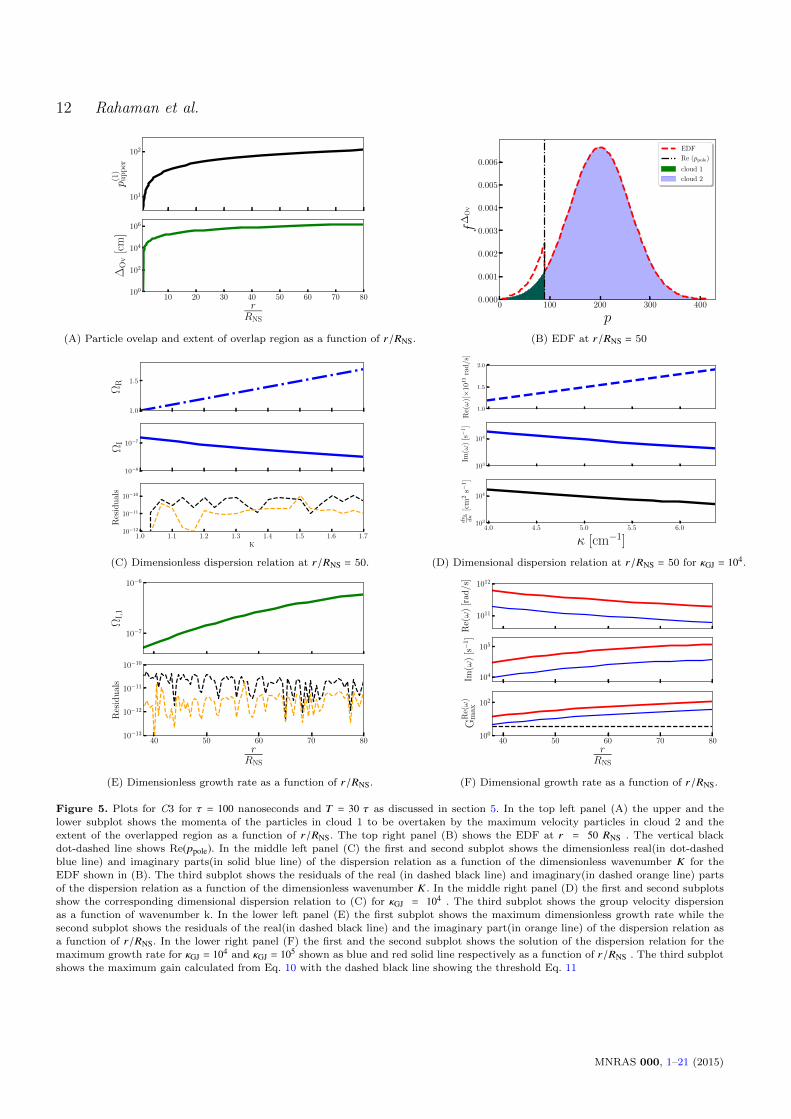
The solution of the dispersion relation does not carry in-formation about the amplitude of the Langmuir wave i.e,we can only calculate eG given the growth rate and the timeavailable for growth. The amplitude is given by E(t) = E(t =0) eG. The initial amplitude E(t = 0) of the wave at a partic-ular frequency has to be obtained from a different treatmentof the dispersion function as is done in subsection C1 of Ap-pendix C. However, since the Langmuir wave grows at theexpense of the particles in the plasma, the maximum energythat the wave can gain is equal to the total energy of allthe particles in the plasma. Thus although the linear the-ory can predict arbitrary gain, in reality, there exists a gainthreshold which cannot be exceeded. The next paragraphdescribes how to get an estimate of this threshold from con-sideration of maximum energy available in the plasma. Ifthe linear theory predicts a gain close to or higher than thisthreshold, then it must be taken as a definitive indicator ofthe breakdown of the linear theory.

To indicate the breakdown of the linear theory we pro-pose the following hypothetical situation: The growth ratesare sufficient for breakdown of linear theory if the lineartheory predicts the energy density in the field to be equalto the total energy density. Let us consider the dispersionrelation for a wave of frequency ωA

1 at two points ‘A’ and‘B’ with point ‘B’ higher up along a given field line. As-suming a constant growth rate the field energy density at

point ‘B’ for ωA1 should satisfy the condition |EωA

1|2B/8π ≈

(|EωA1|2A/8π) e2Gmax = WB where WA and WB are the total en-

ergy density at points “A” and “B”. Using Eq. C9 from Ap-pendix C we obtain a threshold gain indicating the break-down of the linear regime viz., GTh

max ≈ ln[∑

α γ2α

]/2. For

high energy beam driven instability this threshold is dic-tated by the Lorentz factor of the high energy beams. Thegain threshold for instability in case C1 driven by e± beamand the ion beam comes out to be 12 and 6 respectively.The gain threshold for cases C2 and C3 involving only thespecies in the secondary plasma is given by 5. Thus, in allthree cases C1,C2, C3 a representative threshold of gain toindicate the breakdown of linearity can be taken as

GThmax = 5 (11)

4 ESTIMATION OF GROWTH RATES ANDGAIN

In what follows all analyses will be done along the last openfield line of an aligned rotator with period P = 1 second andglobal dipolar strength Bd = 1012 Gauss. For case C1 weget an analytical estimate of the maximum gain. For casesC2 and C3 the hydrodynamic equations Eq. A18 are solvednumerically ( see Appendix D ) to obtain growth rates andmaximum gain as a function of r/RNS.

4.1 C1: Beam-driven Growth

The beam distribution function is given by

f (0)b =1

√πpTb

e−(pb−pb)2/p2

Tb (12)

such that µb = p and σb = pTb/√

2. Further let us introducethe width to mean ratio given by

xb =pTbγb

(13)

From subsection 3.3 the maximum gain for a particularfrequency ωA is given by

Gbmax = ΓωA

( rAc

) [(∆ΩB + 1ΩA

)2/3− 1

]Combining this with expressions for bandwidth of growingwaves (from subsection C2 of Appendix C ) and the thresh-old Eq. 7 we obtain the expression for the maximum gainfor Langmuir waves of frequency ωA

1 due to beam-driveninstability as

Gbmax ≈ xb

pTb

γb2rAc

[8xb3

(γsγb

)2]ωA

1 (14)

4.1.1 High energy positron/electron beam with γb ∼ 106

Egorenkov et al. (1983) demonstrated that only the hydro-dynamic regime exists for the high energy e+/e− beam even

MNRAS 000, 1–21 (2015)


10 20 30 40 50rRNS

10−7

10−5

10−3

10−1

Gm

ax

Figure 1. Plot for maximum gain that can be obtained for

high energy beam driven instability. The dashed red line andthe solid blue line gives the maximum gain for an ion beam and

positron/electron beam with xmin, ion = 0.01 and xe+/e− = 0.3 . A

multiplicity factor of κGJ = 104 and γs = 200 has been used.

for a broad distribution function or large xb. To estimate thegain we chose a representative value xb,e+/e− = 0.3 in Eq. 14and get Gmax,e+/e− , which is plotted as solid blue curve inFig.1 as a function of r/RNS.

4.1.2 High energy ion beam with γion ∼ 103

Unlike the e+/e− beam case, there is no apriori informa-tion indicating for what value of xion will the hydrodynamicregime exist exclusively. Thus to proceed we get an esti-mate of ‘xmin,ion’ for which the kinetic regime gets suppressedcompletely. We assume the ion beam to be composed ofiron ions such that ns/nion = κGJ ∼ 104 , γion/γs ∼ 10 ,mion/me ∼ 56 and Qion/Qe ∼ 26. By substituting Eq. 12in Eq. 5 and estimating it at p =

√2pTb , we have the

maximum dimensionless growth rate in the kinetic regimeΓmax

kin ≈√π/2(χionγ3

ion/8p2T,ione2 χsγ3

s ). Γmaxkin so obtained must

follow the constraint Γmaxkin ≤ pT,ion/γ3

ion. This gives xb,ion ≥[√π/2(nionQ2

ionmeγ3ion/8e22nsQ2

emion γ3s )]1/3 ≈ 0.01. Substitut-

ing xmin,ion = 0.01 in Eq. 14 we get Gmax,ion plotted as dashedred line in Fig.1 as a function of r/RNS. As evident in thefigure, the maximum gain for the ion is larger than thee+/e− beam, however still significantly smaller than the gainthreshold given by Eq. 11.

It can be seen from Fig. 1 that none of the high energybeams can exceed the gain threshold given by Eq. 11.

4.2 C2: Growth due to longitudinal drift

CR77 suggested that due to the motion of the combinedsystem of “beam + secondary plasma” along curved mag-netic field lines , the electron-positron distribution functionin secondary plasma has to separate to provide a steadystate current dictated by the local Goldreich-Julian valueand the solenoidal nature of current flow. The separation of

the bulk velocity ∆β of the species in the secondary plasmaat a distance of rA from the neutron star surface is given by

|∆β|A ≈( ρbρs

)o

[(ΩRot · B fRot)A(ΩRot · B fRot)o

− 1] (15)

where ρb and ρs correspond to the charge density of thebeam and secondary plasma respectively. The ratio (ρb/ρs) =1/κGJ , which we call as the density term. Here the referencepoint “ O” is taken at r = 1.02 RNS where pair creationcascades ceases, a. The correction ‘ fRot ≈ 1 + O(Ω2r2/c2)’due to rotation can be taken to be 1, as the higher orderterm O(Ω2r2/c2) ∼ 0.01 at r = 50RNS for a pulsar withP = 1 second. It can be seen that the separation of theelectron-positron distribution function is a product of twoterms viz., the density term (ρb/ρs)o and the geometricalterm [(ΩRot · B)A/(ΩRot · B)o − 1]. The geometrical factor iszero only for very straight magnetic field lines. Thus curvedmagnetic field line is a necessary requirement of longitudinaldrift/ separation of e± distribution in a secondary plasma.

Simulating EDF for C2: Eq. 15 just gives the dif-ference between β(+) and β(−). To solve for β(+) and β(−) weneed an additional constraint. We make the simplifying as-sumptions that [i] longitudinal drift affects only the meanof the distribution functions i.e, the separation of the bulkvelocity is equal to the separation of the mean of the e±

distribution functions; and [ii] The e± distribution functionsare co-incident at “O” with mean lorentz factor γO

(±) and at

any point rA the mean of the distribution functions separateto attain values that are symmetrical about γO

(±).

The requirement of symmetry translates to the condi-tion that for any other point ‘A’ along the field line∆γ(+) = ∆γ(−) = |∆γ | = γA

(±) − γO(±)

(16)

where γO(±) is the mean of the overlapped distribution func-

tion at point “O” and γA(±) is the mean of the electron-

positron distribution function at “A”.

Let the beta value corresponding to the bulk velocityof both the electrons and positrons at ‘O’ be denoted by βo.For any other point ‘A’, let the beta factor corresponding tothe bulk velocity of the positrons and electrons be denotedby β(+) and β(−), then β(+) − β(−) = [β0 +∆β(+)]− [β0 −∆β(−)]is given by

∆β = ∆β(+) + ∆β(−) (17)

Let us introduce the factor ‘ fratio’ given by ∆β(+) =fratio ∆β(−) and perform the following steps to get the sep-aration (2∆γ) at any distance rA. For a given mean lorentzfactor γO

(±) at ‘O’, and the density term(= 1/κGJ) and ge-

ometrical factor at “A”, Eq. 17 is solved for fratio so as tosatisfy the symmetry constraint given by Eq. 16. Once fratiois obtained, the bulk velocity for the separated distributionfunctions can be estimated as β(+) = βo + ∆β fratio/(1 + fratio)and β(−) = βo −∆β/(1 + fratio). The bulk velocity so obtainedare transformed to the mean lorentz factors γ(+) and γ(−)

via the transformation γ(±) = 1/√

1 − β2±. The corresponding

momenta is given by p(±) ≈ γ(±).

MNRAS 000, 1–21 (2015)

8 Rahaman et al.

In this case the EDF consists of the summation of theshifted gaussian distribution functions with mean γ(+) andγ(−). After getting the EDF we follow the steps outlined inAppendix D to solve the hydrodynamic Eq. A18.

We proceed to solve growth rates for two surface mag-netic field configuration viz., a purely dipolar one and multipolar field. For both field configurations we consider the lastopen field line for an aligned rotator and assume secondaryplasma distribution function to be a gaussian ( with meanµ = 250, width σ = 40) at r/RNS = 1.02.

4.2.1 Simple Dipolar Geometry

The results are shown in Fig. 2. The top panel shows (A)the separation of the distribution functions as a function ofr/RNS for two multiplicity factors (κGJ ∼ 50 , 500) and (B)shows the EDF for κGJ = 500 at a distance of 500 km fromthe neutron star surface. In the middle panel (C) the so-lution of the dispersion relation along with the residuals inthe dimensionless form is shown while (D) shows the dimen-sional growth rate along with the group velocity dispersionat r/RNS = 50 for κGJ = 500 . In the last panel (E) the di-mensionless and (F) the dimensional growth rate along withmaximum gain for an unstable wave of a given frequencyis shown as a function of r/RNS. It must be noted that theRe (ω) does not satisfy the constraint given in section(2.3.1).

4.2.2 Multi-polar Geometry

Simulating the multipolar field configuration: As dis-cussed in section 2.3 any multipolar field configuration mustsatisfy the following two conditions for CCR : [i] At theradio emission heights the pulsar magnetic field must havea purely dipolar character ; [ii] The neutron surface musthave a much smaller radius of curvature ρc compared to apurely dipolar field. As a model for surface multipolar mag-netic field we employ the prescription by Gil et al. (2002).In this model the magnetic field configuration is a super-position of two dipoles viz., a star centred global dipolewith strength Bd and a crust-anchored local dipole embed-ded within ∆R = 0.05RNS from the surface with dipolestrength Bs = bBd. This local component is situated at theco-ordinates (θm, θr) with respect to the global dipole field(see fig.1 of Gil et al. 2002). The strengths of the magneticmoments of the global dipolar field and the local crustal fieldis given by | ®d | = 0.5 BdR3

NS and | ®m| = 0.5 Bm(0.05RNS)3respectively. The boundary condition is chosen such that atthe radio emission region r/RNS = 10 the composite mag-netic configuration should satisfy condition[i]. The middlepanel of Fig. 3 shows ρc as a function of r/RNS for a purelydipole field ( shown in dashed green line ) and a compositeconfiguration (shown as a solid red line) for certain modelparameters are given in the caption. It can be seen that ρcdue to the multi-polar configuration satisfies condition [ii]at the surface. Both ρc and the strength of the magneticfield Btot shown in the middle and the lower panel of Fig. 3resembles that of a purely dipolar configuration within 10

km from the surface. The magnetic field strength for themultipolar configuration differs from that of a purely dipo-lar configuration by less than 0.8% at r/RNS = 2. Thismeans that the superposed field configuration is insensitiveto any change in the boundary condition beyond few tensof km from the surface. Since the multi-polar configurationhas ρc ∼ 105 cm, we can justifiably use high κGJ. It must benoted that for r/RNS ≥ 2 both ρc and Btot attain a purelydipolar character while the geometrical factor quickly at-tains a boosted steady value compared to a purely dipolarsurface geometry as shown in the upper panel of Fig. 3. Thissimulated geometrical factor and high κGJ are then used asinputs for simulating the EDF.

The results of our analysis are shown in Fig. 4 and theplot description are similar to Fig 2 and the parameters forthe simulations are described in the caption to the figure.It is important to note that in this case, unlike the dipolarexample above, Re (ω) satisfy the constraint given in sec-tion(2.3.1).

To summarize as seen in the bottom panel of figures4.2.1 and 4.2.2 sufficient growth rates exceeding the thresh-old limit Eq. 11 can be obtained for both dipolar and mul-tipolar field configuration.

4.3 C3: Growth due to cloud-cloud overlap

This model by Usov (1987) later developed by Ursov & Usov(1988) is based on the non-steady sparking discharge model(also referred to Inner acceleration gap model or the purevacuum gap model) by RS75. In the RS75 model for pul-

sars with ®ΩRot · ®B < 0, positive charges are needed to screenthe co-rotational electric field above the polar cap. Howeverdue to the high binding energy of the ions supply to posi-tive charges are inhibited, and a vacuum gap with a strongelectric field develops above the polar cap. The gap initiallygrows, however, once it reaches a height h ≈ 60 − 100 m,it discharges via magnetic pair creation. Due to the strongelectric field in the gap, the electrons are accelerated to-wards the stellar surface, while the positron streams rela-tivistically away from the stellar surface. The upstreamingpositron has sufficient energy to produce pair cascade, thuscreating the secondary plasma cloud. This process contin-ues until the electric field in the gap is screened, and hencefor the gap emptying time h is a time τ = h/c ∼ which isabout a few hundreds of nanoseconds, the sparking processstops. Once the gap empties, the electric field grows and thesparking process starts again. Hence during steady-state, anon-stationary flow of secondary plasma cloud is generated,with each cloud having a spread in particle velocity. In theoriginal model of Ursov & Usov (1988) the overlap of thefastest and slowest particles of these successive secondaryplasma clouds leads to two-stream instability.

AM98 extended the cloud-cloud overlap formalism ofUrsov & Usov (1988) by categorizing the particles in eachcloud of the secondary plasma into fast, slow and intermedi-ate particles based on their speeds v. The authors presentedan analytical expression for EDF in the overlapped region

MNRAS 000, 1–21 (2015)


0.00

0.01

∣ ∣ ∣Ω

RotB

(ΩR

otB

) O−

1∣ ∣ ∣

0

1

f rat

io

10 20 30 40 50 60 70 80rRNS

0

200

|∆γ|

100 200 300 400 500 600

p

0.000

0.002

0.004

0.006

0.008

0.010

f(0

)α

EDF

Re(ppole)

electron

Positron

(A) Splitting of the distribution function in dipolar geometry (B) EDF at r/RNS =50 for κGJ = 500.

1.0

1.2

1.4

ΩR

10−7

10−6

10−5

ΩI

1.00 1.05 1.10 1.15 1.20 1.25 1.30

K

10−14

10−12

10−10

Res

idu

als

4× 1010

5× 1010

6× 1010

Re(ω

)[r

ad/s

]104

105

2× 1043× 1044× 1046× 104

Im(ω

)[s−

1]

1.40 1.45 1.50 1.55 1.60 1.65 1.70 1.75 1.80

κ [cm−1]

105

2× 105

3× 105dv g dκ

[cm

2s−

1]

(C) Dimensionless dispersion relation at r/RNS = 50 for κGJ = 500. (D) Dimensional dispersion relation at r/RNS = 50 for κGJ = 500.

10−7

10−5

ΩI,

1

10−14

10−11

Res

Re(

DR

)

35 40 45 50 55 60 65 70rRNS

10−14

10−11

Res

Im(D

R)

1010

1011

Re(ω

)[r

ad/s

]

104

105

Im(ω

)[s−

1]

35 40 45 50 55 60 65 70r

RNS

100

101

GR

e(ω

)m

ax

(E) Dimensionless growth rate as a function of r/RNS. (F) Dimensional growth rate as a function of r/RNS.

Figure 2. Plots for C2 longitudinal drift for a purely dipolar geometry as discussed in sections 4.2 and 4.2.1. Left top panel (A) has threesubplots, and from top to bottom shows the geometrical factor, the fratio and ∆γ as a function of r/RNS. The red and blue line corresponds

to κGJ = 50 and κGJ = 500 respectively. The top right panel (B) shows the EDF at r/RNS = 50. The vertical black dot-dashed line shows

Re(ppole). The middle left panel (C), top and middle subplot shows the dimensionless real (in blue dash-dot line) and imaginary parts(in solid blue line) of the dispersion relation as a function of the dimensionless wavenumber K corresponding to the EDF shown in (B)

and the black dash-dot line corresponds to the analytical threshold given by Eq. 7. The third subplot shows the residuals of the realand imaginary parts of the dispersion relation by dashed black and orange line respectively. The middle right panel (D) top and middlesubplot is similar to that of panel C and correspond to the dimensional dispersion relation for κGJ = 500. The bottom subplot of (D)shows the group velocity dispersion as a function of wavenumber k. The lower left panel (E) top, middle, and bottom subplot shows the

maximum dimensionless growth rate and the residuals of the real and imaginary part of the dispersion relation as a function of r/RNS.The red and blue lines correspond to multiplicity factors κGJ = 50 and κGJ = 500, and the dashed red and blue lines refer to the threshold

given by Eq. 7. The lower right panel (F), the top and middle subplot shows the maximum growth rate for κGJ = 50 and κGJ = 500 shownas solid red and blue line respectively as a function of r/RNS. The third subplot shows the maximum gain calculated from Eq. 10 with

the dashed black line showing the threshold Eq. 11.

using Ψ = x − vt. The integral of motion Ψ kept track ofthe position of these three categories of particles in eachsecondary plasma cloud. The distribution function for eachcloud is given by F(p, Ψ) = F(p) F(Ψ). The phase functionF(Ψ) modulates the shape of the distribution function F(p)as a function of r/RNS. In our scheme of constructing the

EDF, We assume that F(Ψ) can be ignored within a singlesecondary plasma cloud. We justify this assumption basedon two considerations. Firstly, in the hydrodynamic regime,the dip in the EDF containing Re (ppole) is of paramountimportance. Since the hydrodynamic equations involve inte-gration over the whole distribution functions, the modulated

MNRAS 000, 1–21 (2015)

10 Rahaman et al.

10−8

10−4

[Ω.B

(Ω.B

) O−

1]

10−2

100

102

ρc/

106

cm

1.0 1.2 1.4 1.6 1.8 2.0r

RNS

1011

1012

1013

Bto

t[in

G]

Figure 3. Plot of the geometrical factor , radius of curvatureand magnetic field strength as a function of r/RNS in the first,

second and third panel respectively, for the last open field line

for a pulsar of period P = 1 seconds and global dipolar field ofBd = 1012 gauss. The local crust-anchored surface field has the pa-

rameters b = 10 , θm = −0.01 radians , θr = 0.08 radians such that

|m/d | = 0.0125. The solid red line and the dashed green line showsthe variation of the aforementioned quantities for a multipolar

configuration and a purely dipolar configuration respectively.

shape of the distribution functions is irrelevant. Secondly,the particles being ultrarelativistic, modulation due to F(Ψ)will be very small. This is because the relative phase spreadin a single cloud between the fastest and the slowest parti-cles compared to the average velocity particles is very small(γ2

fastest−γ2slowest)/γ

2fastestγ

2slowest 1. In this work, the shape of

the gaussian distribution function remains unaltered at anyr/RNS. Below we present a more generic way to constructEDF numerically.

Simulating EDF for C3 : Let the gap closingtimescale be ‘τ’. The time required to form a single cloudis ‘T = 30τ’ such that a fully formed spark corresponds toa cloud of electrons and positrons of length Ls = cT . Let usconsider two successive discharges giving rise to a leadingcloud (labelled by index ‘1’) and a trailing cloud (labelledby index ‘2’). Let the distribution function of each secondaryplasma have a maximum and minimum dimensionless mo-menta cut-offs characterized by pmax and pmin respectively.The velocity corresponding to any p in the distribution func-

tion is given by the transformation v = pc/√

1 + p2 such thatthe corresponding cut-off velocities are given by vmax andvmin respectively. Let the particles with arbitrary velocity

in cloud 1 and cloud 2 be labelled by v(1)arb and v

(2)arb respec-

tively. We define the overlap region between the position of

v(2)max and the position of v

(1)min and give a description for the

construction of the EDF below.

The time t in which v(2)max overlaps with v

(1)arb is

tOv =v(1)arbτ −

[v(2)max − v

(1)arb

]T

v(2)max − v

(1)arb

for v(1)upper = v

(1)arb ≥ v

(1)min.

The position of overlap is given by

xOv =v(2)max v

(1)arbτ

v(2)max − v

(1)arb

which can be represented as a function of r/RNS.

The position of the minimum velocity particles of cloud‘1’ at time tOv is given by

x(1)min =v(1)min v

(2)maxτ

v(2)max − v

(1)min

= v(2)lower(T + tOv)

The equality is used to solve for v(2)lower and the solution trans-

formed to dimensionless momenta p(2)lower via the transforma-

tion p = β/√

1 − β2.

The EDF f Ov in the overlapped region is given by

f Ov = f1 [p(1)min : p(1)upper] + f2 [p(2)lower : p(2)max]

where the notation fn[a : b] refers to the portion of distribu-tion function fn from a to b for cloud with index ‘n’.

The spatial extent of the overlapped region is given by

∆Ov = x(2)max − x(1)min =

[v(2)max v

(1)min − v

(1)minv

(2)max

]τ

v(2)max − v

(1)min

The dispersion relation in the overlapped region is givenby the expression

1 − χ∫ +∞−∞

dpf ∆Ov

γ31

(Ω − βK)2= 0 (18)

In this case, the EDF is being determined by the lowerand higher momenta cut-off pmin and pmax of the secondaryplasma distribution function and the gap closing time τ.Here we assume a gaussian distribution function with µ =

200, σ = 60, pmin = 5, pmax = 400 for the secondary plasmaclouds.After getting the EDF we follow the steps outlinedin Appendix D to solve the hydrodynamic equations. Theresults of our numerical solution are shown in Fig. 5. As seenfrom the third subplot of (F) sufficient growth rates can beobtained exceeding the gain threshold defined in section 3.4.

4.3.1 Effect due to longitudinal drift

In the previous numerical simulation we have taken the valueof pmin = 5. However, if this value were to be higher the con-tribution to the EDF at a given height due to the leading

cloud f1 [p(1)min : p(1)upper] becomes smaller which decreases thedimensionless growth rate drastically. We consider a situa-tion where for some orientation of the crust-anchored dipoleand high κGJ, the longitudinal drift can lead to splitting inthe electron-positron distribution function in the secondaryplasma but does not produce minima in the EDF for C2.

However when combined with C3 this separation lowers p(1)minof the distribution functions as the cloud flows outward alongthe field line. We perform the next numerical simulation to

MNRAS 000, 1–21 (2015)


0.0

0.2

∣ ∣ ∣Ω

RotB

(ΩR

otB

) O−

1∣ ∣ ∣

0.25

0.50

f rati

o

10 20 30 40 50 60 70 80r

RNS

50

100

|∆γ|

100 200 300 400 500 600

p

0.000

0.002

0.004

0.006

0.008

0.010

f(0

)α

EDF

Re(ppole)

electron

Positron

(A) Splitting of the distribution function in multipolar geometry. (B) EDF at r/RNS = 50 for κGJ = 104.

1.0

1.2

1.4

ΩR

10−7

10−6

ΩI

1.00 1.05 1.10 1.15 1.20 1.25 1.30

K

10−14

10−12

10−10

Res

idu

als

2× 1011

3× 1011

Re(ω

)[r

ad/s

]

105

4× 1046× 104

2× 1053× 1054× 105

Im(ω

)[s−

1]

6.50 6.75 7.00 7.25 7.50 7.75 8.00

κ [cm−1]

4× 103

5× 103

6× 103

7× 103dv g dκ

[cm

2s−

1]

(C) Dimensionless dispersion relation at 500 km for κGJ = 104. (D) Dimensional dispersion relation at r/RNS = 50 for κGJ = 104.

10−6

6× 10−7

2× 10−6

ΩI,

1

10−14

10−11

Res

Re(

DR

)

40 50 60 70 80rRNS

10−13

10−11

Res

Im(D

R)

1011

2× 1011

3× 1011

4× 1011

Re(ω

)[r

ad/s

]

105

2× 105

3× 1054× 105

Im(ω

)[s−

1]

35 40 45 50 55 60 65 70r

RNS

100

102

GR

e(ω

)m

ax


Figure 4. Plots for C2 along the last open field line for a multi-polar field configuration parameters (see Fig. 3 ) as discussed in section

4.2.2. The plot description is the same as for Fig.2 with the red and blue lines representing κGJ = 8×103 and 104 respectively.

study the effect of longitudinal drift on the cloud-cloud over-lap for the aforementioned scenario. The results are shownin Fig. 6. As seen from the third subplot of (F) even in thishybrid of cases C2 and C3 the maximum gain exceeds thegain threshold defined in section 3.4.

We find that in the absence of C2 the dimensionlessgrowth rate (ΩI < 10−8 ) and comparable to the residuals ofthe hydrodynamic equations.

5 DISCUSSION AND COMPARISONS WITHPREVIOUS STUDIES

In sections 3 and 4 we provided a hot plasma treatment oftwo-stream instability and estimated growth rates of Lang-muir mode for various models of one-dimensional plasmaflow in pulsars. Based on our analysis our final aim is to ex-amine under what conditions excitation of CCR is possiblein pulsars. There are at least three conditions, namely, (I),(II) and (III) that need to be fulfilled. The first condition (I)is that for two-stream instability to occur in one-dimensionalplasma flow, the EDF should not be single-humped (Gard-ner’s theorem). If condition (I) is satisfied, excitation of CCRfurther requires the following two constraints to be satisfiedsimultaneously viz., (II) The amplification criteria which re-

MNRAS 000, 1–21 (2015)

12 Rahaman et al.

101

102

p(1)

up

per

10 20 30 40 50 60 70 80rRNS

100

102

104

106

∆O

v[c

m]

0 100 200 300 400

p

0.000

0.001

0.002

0.003

0.004

0.005

0.006

f∆

Ov

EDF

Re (ppole)

cloud 1

cloud 2

(A) Particle ovelap and extent of overlap region as a function of r/RNS. (B) EDF at r/RNS = 50

1.0

1.5

ΩR

10−8

10−7

ΩI

1.0 1.1 1.2 1.3 1.4 1.5 1.6 1.7K

10−12

10−11

10−10

Res

idu

als

1.0

1.5

2.0

Re(ω

)[×

1011

rad/s

]103

104

Im(ω

)[s−

1]

4.0 4.5 5.0 5.5 6.0

κ [cm−1]

103

104

dv g dκ

[cm

2s−

1]

(C) Dimensionless dispersion relation at r/RNS = 50. (D) Dimensional dispersion relation at r/RNS = 50 for κGJ = 104.

10−7

10−6

ΩI,

1

40 50 60 70 80rRNS

10−13

10−12

10−11

10−10

Res

idu

als

1011

1012

Re(ω

)[r

ad/s

]

104

105

Im(ω

)[s−

1]

40 50 60 70 80rRNS

100

102

GR

e(ω

)m

ax


Figure 5. Plots for C3 for τ = 100 nanoseconds and T = 30 τ as discussed in section 5. In the top left panel (A) the upper and thelower subplot shows the momenta of the particles in cloud 1 to be overtaken by the maximum velocity particles in cloud 2 and theextent of the overlapped region as a function of r/RNS. The top right panel (B) shows the EDF at r = 50 RNS . The vertical black

dot-dashed line shows Re(ppole). In the middle left panel (C) the first and second subplot shows the dimensionless real(in dot-dashedblue line) and imaginary parts(in solid blue line) of the dispersion relation as a function of the dimensionless wavenumber K for the

EDF shown in (B). The third subplot shows the residuals of the real (in dashed black line) and imaginary(in dashed orange line) parts

of the dispersion relation as a function of the dimensionless wavenumber K . In the middle right panel (D) the first and second subplotsshow the corresponding dimensional dispersion relation to (C) for κGJ = 104 . The third subplot shows the group velocity dispersionas a function of wavenumber k. In the lower left panel (E) the first subplot shows the maximum dimensionless growth rate while thesecond subplot shows the residuals of the real(in dashed black line) and the imaginary part(in orange line) of the dispersion relation asa function of r/RNS. In the lower right panel (F) the first and the second subplot shows the solution of the dispersion relation for the

maximum growth rate for κGJ = 104 and κGJ = 105 shown as blue and red solid line respectively as a function of r/RNS . The third subplotshows the maximum gain calculated from Eq. 10 with the dashed black line showing the threshold Eq. 11

MNRAS 000, 1–21 (2015)


[H]

10−8

10−7

10−6Ω

I,1

45 50 55 60 65 70 75 80rRNS

10−14

10−12

10−10

Res

idu

als

1011

2× 1011

3× 1011

Re(ω

)[r

ad/s

]

104

105

Im(ω

)[s−

1]

45 50 55 60 65 70 75 80r

RNS

10−1

101

GR

e(ω

)m

ax

(A) Dimensionless growth rate as a function of r/RNS. (B) Dimensional growth rate as a function of r/RNS.

Figure 6. Plots for C3 aided by C2 along the last open field line for multi-polar configuration as used in Fig. 3 and discussed in section

4.3.1 . Here τ = 100 nanoseconds and T = 30 τ. A gaussian with µ = 240, σ = 50, pmin = 25, pmax = 400 has been assumed for thedistribution function for the secondary plasma cloud at r = 1.02 RNS. Multiplicity factor of κGJ = 2× 104 has been used. For left panel (A)

the upper subplot shows the maximum dimensionless growth rate as a function of r/RNS. The lower subplot shows the residuals of thereal(in dashed black line) and imaginary(in dashed orange line) parts of the dispersion relation respectively as a function of r/RNS. For

the right panel (B) the upper and the middle subplot shows real and imaginary part of the dispersion relation in its dimensional form as

a function of r/RNS. The lower subplot shows the maximum gain obtained using Eq. 10 as a function of r/RNS. The dashed black line inthe second subplot of (B) represents the threshold Eq.11

−0.05 0.00 0.05

θm [rad]

−0.075

−0.050

−0.025

0.000

0.025

0.050

0.075

θ r[r

ad]

20

40

60

80

100

120

−0.05 0.00 0.05

θm [rad]

−0.075

−0.050

−0.025

0.000

0.025

0.050

0.075

θ r[r

ad]

5

10

15

20

25

(A) Color map for κGJ = 104 at r/RNS = 50 (B) Color map for κGJ = 105 at r/RNS = 50

Figure 7. Color map showing the separation (∆γs) of the electron-positron distribution function due to longitudinal drift at r/RNS =50 due to various orientation (θm, θr) of the crust-anchored field (b = 10, Bd = 1012gauss) as shown in fig. 1 of Gil et al. 2002. The mean

value of the gaussian is taken to be γs = 250 and the ratio of dipole moments of the crust-anchored dipole to global dipole star centred

dipole has been fixed to |m/d | = 1.25 × 10−3. For σ = 40, the separation is said to be sufficient only if ∆γs >= 1.5σ.

quires the maximum gain Gmax to be greater than a gainthreshold (see Eq. 11 ), and (III) The brightness tempera-ture criteria which requires a very dense plasma. Condition(III) requires the scaling factor ω1 to satisfy threshold cri-teria given by Eq. 8.

Note that the estimation of gain requires the descrip-tion of EDF and the scaling ω1. The solutions of the dimen-sionless hydrodynamic equation are determined by the EDFand subsequently one obtains the dimensionless growth rate(ΩI) and the bandwidth of growing waves(∆ΩR). The dimen-sional growth rate(ωI) is a product of ΩI and ω1. The scalingfactor varies as ω1 ∝

√κGJ nGJ and falls monotonically with

distance. Thus to satisfy condition(III) high κGJ is necessary,which requires multi-polar surface magnetic field geometry.In what follows we check how these conditions (II) and (III)

are fulfilled for cases C1, C2 and C3 respectively. We com-pare our results with previous studies and discuss furtherimplications.

5.1 Results for C1

Observations suggest the presence of an ion component inpulsar plasma (see Gil et al. 2003) along with the e+/e+beam. We assume the ion component to be composed ofiron and characterized by a bulk Lorentz factor of γion ≈ 103.While hot plasma treatment for e+/e+ beam exists in the lit-erature, as far as we know that such treatment for an ionbeam does not exist in the literature. We analyze the ioncomponent similarly as Egorenkov et al. (1983) did for the

MNRAS 000, 1–21 (2015)

14 Rahaman et al.

50 60 70 80 90 100 110 120rRNS

10

20

30

40G

Re(ω

)m

ax

80 100 120 140 160 180r

RNS

10

20

30

40

GR

e(ω

)m

ax

(A) Gmax as a function of r/RNS for longitudinal drift. (B) Gmax as a function of r/RNS for cloud-cloud overlap.

0 100 200 300 400 500 600

p

0.000

0.002

0.004

0.006

0.008

0.010

f(0

)α

EDF

Re(ppole)

electron

Positron

0 100 200 300 400

p

0.000

0.002

0.004

0.006

0.008

f∆

Ov

EDF

Re (ppole)

cloud 1

cloud 2

(C) EDF for longitudinal drift in multipolar geometry at r/RNS = 180. (D) EDF for cloud-cloud overlap at r/RNS = 180.

Figure 8. “Window of opportunity” of Cherenkov resonance. The plots for C3 uses τ = 150 nanoseconds and κGJ = 105 with gaussian

distribution function parameters σ = 60, pmin = 5, pmax = 400, pmean = 200. The plots for C2 uses multipolar configuration see fig. 1 of Gil

et al. 2002 with b = 10, θr = 0.08 rad, θm = −0.01 rad, with κGJ = 104 and gaussian distribution function parameters σ = 50, pmean = 240.In the upper panels (A) and (B) the dashed horizontal black line in corresponds to gain threshold given in Eq 11 . The dashed dot

vertical red line corresponds to the density threshold given in Eq.8. The shaded yellow region shows the “Window of Opportunity” where

both these constraints are satisfied. The lower panels (C) and (D) shows the EDF for C2 and C3 at r/RNS = 180. The vertical blackdot-dashed line shows Re(ppole).

high energy e+/e+ beam. We find that for width to mean ra-tio of 1% the kinetic regime is completely suppressed. Usingthis width we estimate the maximum gain for the ion beamin the hydrodynamic regime. For the sake of comparison, wealso estimate the maximum gain for the high energy e+/e−beam. We find that although the gain for the ion beam is ∼5 orders of magnitude higher than e+/e− beam yet it cannotsatisfy condition (II). Since none of the beams can satisfycondition (II) the beam driven Langmuir instabilities areexcluded as candidates for pulsar radio emission.

5.2 Results for C2 and C3

AM98 found that growth rates in C3 exceed that of C2 forthe same κGJ at the radio emission region (see panels (a)and (b) of fig. 6 in AM98). AM98 further asserts that C3dominates C2 below r/RNS = 50 and that the role changesbeyond this distance. In our work we find these assertionsto be inconsistent. We find the exact opposite result as canbe seen from the panel (F) in Fig. 4 and 5 for κGJ = 104.These conflicting results can be understood by comparingthe methodology for the construction of EDF in this workand AM98.

5.2.1 EDF for C2

As discussed in section 4.2 the separation of the bulk-velocities ∆β is equal to the product of the geometrical termand the density term. However, both CR77 and AM98 as-sume the geometrical term to be equal to unity. This as-sumption is not valid at the radio emission region. For bothdipolar and multipolar surface magnetic field geometries, thegeometrical term is much less than unity ( See the uppersubplot in panel A of Fig. 2 and Fig. 4 ).

Further CR77 assumed the radio emission region to besufficiently far from the surface. Assuming a delta-functionfor e+−e− distribution functions they estimated Im (ω) suchthat Re(ω) ≤ ωCCR. This is incompatible with the condi-tion (III). Improving upon the cold plasma approximationof CR77, AM98 presented a hot plasma treatment. But theyincorrectly assumed (in addition to neglecting the geometri-cal term), the same ∆β for different κGJ, whereas a self con-sistent treatment requires different ∆β = 1/κGJ. However, intheir case ΩI is constant since the EDF has been assumedto be the same for different κGJ. Consequently ωI at anyheight scales only as ω1 ∝

√κGJ (shown as vertical shift of

ωI in logarithmic scale in panel(a) of fig.6 of AM98). Thus,AM98 made two inconsistent assumptions for C2. Our work

MNRAS 000, 1–21 (2015)


corrects these assumptions by incorporating mutually con-sistent geometrical terms and κGJ for different kinds of sur-face geometries. As discussed in section 2.3 a low/high κGJshould be associated with purely dipolar/multipolar surfacemagnetic field geometry.

In section 4.2 we considered a purely dipolar surfacegeometry in conjunction with κGJ = 50 and κGJ = 500 andfound that condition(II) is satisfied. However, as seen fromthe first subplot of (F) in the lower panel of Fig. 2, condition(III) is not satisfied. Note that in reality κGJ ∼ 10 − 100for the purely dipolar surface magnetic field case and henceunder no circumstance can condition (III) be satisfied. Wehave shown this case only for the sake of illustration wherecondition (II) and (III) are not satisfied simultaneously.

Apart from being incompatible, using purely dipolarsurface magnetic to get the geometrical factor(∼ 10−3) witha very high κGJ ∼ 104 is unfruitful, as the separation∆β ∼ 10−7 is negligible and condition (I) will not satisfied.However, even for multi-polar surface magnetic field geom-etry, high κGJ necessarily suppresses ∆β such that condition(I) cannot be satisfied. An increase in ∆β can be achievedby only increasing the geometrical term. This effect requires(ΩRot.B)O to be lowered in the geometrical term. To sim-ulate the geometrical term for a multi-polar geometry weuse the prescription of Gil et al. (2002) to model the sur-face using two dipoles viz., the global star-centered dipoleand a local crust anchored dipole with orientation parame-ters (θm, θr) (see subsection 4.2.2 for details). However, notall orientation of the crust-anchored local dipole can lowerthis term. To explore this effect we perform the followingexercise: We change both θm and θr in the range -0.08 radi-ans to + 0.08 radians for a fixed ratio of the dipole moments|m/d | = 1.25×10−3 and trace the last open magnetic field line.Fig. 7 shows the color map of ∆γ for κGJ = 104 and κGJ = 105

in sub-plots (A) and (B) at r = 50RNS for a gaussian dis-tribution function with (mean µ = 250, width σ = 40) atr/RNS = 1.02. The separation is taken to be sufficient onlyif ∆γ ≥ 1.5σ. Within this parameter space, the separation issufficient in sub-plot (A) for a few special orientations whilefor sub-plot (B) the separation is insufficient for any orienta-tion. The results for one such orientation in sub-plot (A) areshown in Fig. 4 where panel (F) shows both conditions (II)and (III) are satisfied simultaneously in the radio emissionregion. The geometrical factor for these special orientationsquickly attains an almost constant value beyond a few kmfrom the surface (see the upper panel of Fig. 3) which trans-lates to a near steady EDF for r/RNS ≥ 2. A steady EDFtranslates to a steady ΩI. Thus ωI is completely dominatedby number density via the scaling ω1. This means for fewspecial orientations of the local crust anchored field, bothconditions (II) and (III) are satisfied simultaneously beyondfew tens of km from the surface. This is an essentially newresult that has been obtained using a very thorough anal-ysis of the geometrical term. It must also be pointed thatfor the same geometrical term the growth rates and gain de-pend sensitively on κGJ as shown in Fig. 4 for κGJ = 104 andκGJ = 8 × 103.

5.2.2 EDF for C3

AM98 constructed the EDF at a few r/RNS (see Table 2 ofAM98) for which the shape of the EDF does not change andextrapolated the results in between. In their analysis, ΩI re-mains fixed and the growth rate (ωI) falls monotonically asthe scaling ω1 (see panel (b) of fig.6 in AM98). Panel (b)of fig.6 in AM98 also shows ωI to be high even for moder-ately low κGJ ∼ 102−103. However, both these assertions areincomplete and invalid as is discussed below. Many impor-tant features have been missed in AM98 due to the coarseresolution of their numerical simulations.

We find that the variation of the growth rate ωI as afunction of r/RNS in C2 is not monotonic. It can be dividedinto two distinct spatial regions - the first part is dominatedby the EDF and the later part by the number density viaω1. Although the overlap of the distribution functions be-gins very close to the neutron star at r ≈ 2p2

mincτ ∼ 1.5 km,ωI remains very low until a few hundred km from the sur-face. It is in this very regime that AM98 incorrectly assertsthat C3 will dominate C2. We find that ΩI remains very low2( 10−8) until a substantial contribution ( f1 [p(1)min : p(1)upper]) from the leading cloud “1” gives rise to a prominent low-momenta tail in the EDF ( see panel B of Fig. 5 ). As seenfrom panel (A) of Fig. 5, pupper

1 changes slowly beyond a fewhundred km. This implies the shape of the EDF changesrapidly closer to the neutron star and vice versa. Thus asa prominent tail starts developing ΩI first increases rapidlyand then attains a steady value. Consequently for the firstfew hundred km ωI remains very low, followed by a subse-quent increase and then a decline following a turnover. Thepanel (F) of Fig. 5 shows ωI before the turnover. Howevereven after the development of a prominent tail ΩI does notexceed 10−7(see panel E of Fig. 4.3). This necessarily re-quires very high κGJ = 104 − 105 via scaling ω1 to give riseto high growth rates. This is again opposite to what AM98obtained. To conclude we find conditions (II) and (III) aresatisfied simultaneously for C3 only beyond a few hundredkm from the surface and for very high κGJ. This is an es-sentially new result that has been obtained due to the finerresolution of our numerical simulations.

To summarize, for C2 and C3 the coarseness of the nu-merical resolution coupled with many simplifying assump-tions led AM98 to general conclusions which are not validfor realistic pulsar parameters. In this study, we have ad-dressed the inconsistencies of AM98.

5.3 Window of Opportunity(WoU)

We are now interested to find the spatial region along themagnetic field where both conditions (II) and (III) are ful-filled simultaneously, and call this the “Window of Oppor-tunity” (hereafter WoU). WoU is shown as a shaded yellowregion for C2 and C3 in panels (A) and (B) of Fig.8. It canbe seen that for C2, the gain Gmax decreases monotonically

2 see Appendix D for details of numerical simulations

MNRAS 000, 1–21 (2015)

16 Rahaman et al.

while for C3 the gain shows a turnover. As discussed pre-viously the EDF for C2 retains the same shape beyond fewtens of km from the surface. This means the gain curve justreflects the scaling ω1 which decreases monotonically. On theother hand gain curve for C3 is dominated by EDF ( f Ov)before turnover and by scaling ω1 beyond it.

However there is an additional difference between thegain curves of C2 and C3. The EDF for C2 follows condition(I) for all r/RNS ≥ 2, while EDF for C3 follows condition (I)

only till p(1)lower < p(2)mean. For p(1)lower ≥ p(2)mean, the EDF is notsingle humped and consequently ωI ceases. The gain for C3

can go to zero abruptly. Lower the p(2)mean , closer to the neu-tron star surface can this termination occur. In this scenarioabrupt termination in gain can violate condition (II) muchcloser to the neutron star. For our chosen parameters thistermination occurs beyond the distance where both condi-tions conditions (II) and (III) are violated. Panels (C) and(D) in Fig. 8 shows EDF for C2 and C3 at r/RNS = 180,where it can be seen ( compared to panel (B) for Fig. 4 andFig. 5 ) that far from the neutron star surface the dip in theEDF decreases for C3 and remains the same for C2.

In a realistic scenario both C2 and C3 are at work. How-ever, in such a combination the EDF with the greater growthrate dominates. It is clear from the previous discussion forFig. 7 that for high κGJ = 105 and a few orientations of thelocal crust anchored dipole the EDF for C2 cannot satisfythe condition (I). For these situations exclusively C3 can op-erate. As discussed in section 4.3 the EDF for C3 depends onτ and the momenta cut-offs in the distribution functions. Ifp(1)min were to be lower, the contribution f1 [p(1)min : p(1)upper] fromthe leading cloud becomes smaller at a given height. This

then decreases ΩI. However when combined with C2 p(1)mindecreases with height which then increases the contributiondue to f1. The results for such a hybrid scenario are shown inFig. 6 where it is seen that both conditions (II) and (III) aresatisfied. Thus, a variety of combinations of C2 and C3 cansatisfy conditions (II) and (III) simultaneously, thereby giv-ing the“WoU”. It must also be noted that our conclusions arevalid only for a strictly one-dimensional plasma flow whereonly the Cherenkov resonance condition operates. This as-sumption is not valid very far away from the neutron starsurface where curvature drift (viz., the flow of particles per-pendicular to the magnetic field plane ud ≈∼ v2

‖γ/ωB,α ρc ;

see Kazbegi et al. 1991) will set in.

We suggest the presence of WoU can be applied toexplain the phenomenon of Radius-to-Frequency mappingwhere radio emission appears to arise from a range of emis-sion heights. The variation of the gain curve can be used toexplain time-variable features in pulsar radio emission likemoding and nulling. These aspects will be addressed in fu-ture work.

5.4 Choice of the distribution functions

We have adopted a semi-numerical approach in this workwhere we have assumed the distribution functions of thespecies in plasma to be gaussians. The mean values of sec-

ondary plasma distribution functions reflect the order ofmagnitude estimate derived from considerations of CCR.Recently the choice of relativistically streaming gaussianshas been criticized by Rafat et al. (2019). For C2 the sym-metric nature of the gaussian distribution function allowedthe bulk velocity to be associated with the mean. This al-lowed us to construct EDF for C2 by only shifting the meanswithout changing the shape. For an asymmetric distributionfunction, no such prescription exists and the shape of thee+ − e− distribution functions can get distorted while sepa-rating. This can affect the dip in the EDF and consequentlythe growth rate (see the first paragraph in Appendix D).However, for C3 even for a non-gaussian distribution func-tion the most relevant parameters would still be the locationof the peak and pmin. The generic features of the amplifica-tion curve for C2 and C3 as shown in Fig. 8 would not changewith the change in the distribution function. The detailedaspects of WoU for different distribution functions will beaddressed in a future study.

6 CONCLUSION

In this study, we find that both C2 and C3 can lead to ex-citation of large amplitude Langmuir waves, while the sec-ondary plasma should be dense enough to account for highTb in CCR. Contrary to the results obtained by AM98, wefind that for certain multipolar surface magnetic field con-figurations, the amplification gain for C2 vastly exceeds thatof C3 for the same κGJ. For these special configurations, veryhigh amplification can be achieved very close to the neutronstar and the spatial extent over which C2 operates vastlyexceeds that due to C3. A generic feature for C3 is that thegain becomes high only for κGJ ≥ 104 after a few hundredkm from the neutron star surface. For κGJ ∼ 105 C3 operatesexclusively as growth rates in C2 are suppressed completely.For surface field configurations and high κGJ wherein theEDF for C2 is single-humped, the separation neverthelessaids C3 by enhancing the low momenta tail in the EDF forC3. We find a window of opportunity (WoU) of Cherenkovresonance around r/RNS ∼ 100 where any combination ofC2 and C3 can account for CCR. The presence of large am-plitude Langmuir waves in WoU provides an impetus for ahigher-order plasma theory.

ACKNOWLEDGEMENT

We thank the anonymous referee for critical comments andsuggestions that helped to improve the manuscript signifi-cantly. We thank Rahul Basu from IUCAA for discussionsand suggestions. We thank Marina Margishvili for carefulreading of the manuscript, suggestion and support. Sk. MRand DM acknowledge the support of the Department ofAtomic Energy, Government of India, under project no. 12-R&D-TFR-5.02-0700. DM acknowledges support and fund-ing from the “Indo-French Centre for the Promotion of Ad-vanced Research - CEFIPRA” grant IFC/F5904-B/2018.

MNRAS 000, 1–21 (2015)


DATA AVAILABILITY

The data from the numerical simulations will be shared onreasonable request to the corresponding author, Sk. Min-hajur Rahaman.

REFERENCES

Arendt, Paul N. J., Eilek J. A., 2002, ApJ, 581, 451

Arons J., Barnard J. J., 1986, ApJ, 302, 120

Arons J., Scharlemann E. T., 1979, ApJ, 231, 854

Arumugasamy P., Mitra D., 2019, MNRAS, 489, 4589

Asseo E., Melikidze G. I., 1998, MNRAS, 301, 59

Benford G., Buschauer R., 1977, MNRAS, 179, 189

Blasi P., Amato E., 2011, Astrophysics and Space Science Pro-ceedings, 21, 624

Blaskiewicz M., Cordes J. M., Wasserman I., 1991, ApJ, 370, 643

Cheng A. F., Ruderman M. A., 1977, ApJ, 212, 800

Cordes J. M., 1979, Space Sci. Rev., 24, 567

de Jager O. C., 2007, ApJ, 658, 1177

Egorenkov V. D., Lominadze D. G., Mamradze P. G., 1983, As-trofizika, 19, 753

Force M. M., Demorest P., Rankin J. M., 2015, MNRAS, 453,4485

Gardner C. S., 1963, Physics of Fluids, 6, 839

Gedalin M., Gruman E., Melrose D. B., 2002, MNRAS, 337, 422

Gil J., Lyubarsky Y., Melikidze G. I., 2004, ApJ, 600, 872

Gil J., Melikidze G. I., Geppert U., 2003, A&A, 407, 315

Gil J., Mitra D., 2001, ApJ, 550, 383

Gil J. A., Melikidze G. I., Mitra D., 2002, A&A, 388, 235

Ginzburg V. L., Zhelezniakov V. V., 1975, ARA&A, 13, 511

Ginzburg V. L., Zheleznyakov V. V., Zaitsev V. V., 1969, Ap&SS,

4, 464

Goldreich P., Julian W. H., 1969, ApJ, 157, 869

Hibschman J. A., Arons J., 2001, ApJ, 560, 871

Jackson J. D., 1962

Johnston S., Hobbs G., Vigeland S., Kramer M., Weisberg J. M.,

Lyne A. G., 2005, MNRAS, 364, 1397

Kazbegi A. Z., Machabeli G. Z., Melikidze G. I., 1991, MNRAS,253, 377

Kellermann K. I., Pauliny-Toth I. I. K., 1969, ApJ, 155, L71

Lai D., Chernoff D. F., Cordes J. M., 2001, ApJ, 549, 1111

Lakoba T., Mitra D., Melikidze G., 2018, MNRAS, 480, 4526

Lominadze D. G., Machabeli G. Z., Melikidze G. I., PataraiaA. D., 1986, Fizika Plazmy, 12, 1233

Lominadze D. G., Mikhailovskii A. B., 1979, Soviet Journal ofExperimental and Theoretical Physics, 49, 483

Lyutikov M., 1999, Journal of Plasma Physics, 62, 65

Lyutikov M., 2000, MNRAS, 315, 31

Medin Z., Lai D., 2010, MNRAS, 406, 1379

Melikidze G. I., Gil J. A., Pataraya A. D., 2000, ApJ, 544, 1081

Melikidze G. I., Mitra D., Gil J., 2014, ApJ, 794, 105

Melrose D. B., 1978, ApJ, 225, 557

Melrose D. B., 1993, in Pulsars as Physics Laboratories, ShullJ. M., Thronson H. A., eds., pp. 105–115

Melrose D. B., Gedalin M. E., 1999, ApJ, 521, 351

Mitra D., 2017, Journal of Astrophysics and Astronomy, 38, 52

Mitra D., Basu R., Melikidze G. I., Arjunwadkar M., 2020, MN-RAS, 492, 2468

Mitra D., Gil J., Melikidze G. I., 2009, ApJ, 696, L141

Mitra D., Li X. H., 2004, A&A, 421, 215

Mitra D., Rankin J. M., 2002, ApJ, 577, 322

Mitra D., Rankin J. M., 2011, ApJ, 727, 92

Noutsos A., Kramer M., Carr P., Johnston S., 2012, MNRAS,

423, 2736

Noutsos A., Schnitzeler D. H. F. M., Keane E. F., Kramer M.,

Johnston S., 2013, MNRAS, 430, 2281

Pataraia A., Melikidze G., 1980, Ap&SS, 68, 49

Rafat M. Z., Melrose D. B., Mastrano A., 2019, Journal of PlasmaPhysics, 85, 905850603

Rankin J. M., 1993, ApJ, 405, 285

Rankin J. M., 2007, ApJ, 664, 443

Ruderman M. A., Sutherland P. G., 1975, ApJ, 196, 51

Suvorov E. V., Chugunov I. V., 1975, Astrofizika, 11, 305

Szary A., Melikidze G. I., Gil J., 2015, MNRAS, 447, 2295

Timokhin A. N., Harding A. K., 2019, ApJ, 871, 12

Ursov V. N., Usov V. V., 1988, Ap&SS, 140, 325

Usov V. V., 1987, ApJ, 320, 333

Usov V. V., 2002, in Neutron Stars, Pulsars, and Supernova Rem-nants, Becker W., Lesch H., Trumper J., eds., p. 240

von Hoensbroech A., Xilouris K. M., 1997, A&AS, 126, 121

Weltevrede P., Johnston S., 2008, MNRAS, 391, 1210

Young M. D., Manchester R. N., Johnston S., 1999, Nature, 400,

848

This paper has been typeset from a TEX/LATEX file prepared by

the author.

The following appendix is being provided for an expanded

discussion and derivations that has been used extensively in themain paper.

APPENDIX A: MAKING USE OF THELANDAU PRESCRIPTION FORELECTROSTATIC MODE FOR AONE-DIMENSIONAL RELATIVISTIC PLASMA

In the sub-Luminal region we make use of the Landau Prescrip-tion where we allow ω to be complex and hence the integral in

the dispersion relation can be replaced by a contour integral to

give

κc +∑α

ω2p,α

∮Ldpα

∂ f(0)α

∂pα

1(ω − βακc)

= 0 (A1)

where L stands for the Landau Contour.

Thus we have a pole at a value of particle three momenta

ppole =ω√

(κc)2 −ω2(A2)

Since ω can now be complex we can write

ω = ωR + i ωI (A3)

Thus the pole can be written as

ppole =

(√|U |+a

2 ± i√|U |−a

2

)Q

(A4)

where

|U | =√a2 + b2

a = κ2c2(ω2

R −ω2I

)−

(ω2

R +ω2I

)2

b = 2 ωR ωI (κc)2

Q =√(κc)2

[(κc)2 + 2(ω2

R −ω2I )

]+ (ω2

R +ω2I )2 (A5)

MNRAS 000, 1–21 (2015)

18 Rahaman et al.

Figure A1. Contour diagram for ωI ωR

which gives us

Im (ppole) < 0 if b < 0⇒ ωI < 0Im (ppole) > 0 if b > 0⇒ ωI > 0Im (ppole) = 0 if b = 0⇒ ωI → 0

Thus we can have three cases depending on the sign of ωI. We

are interested in the growth of waves. We explore the two regimesof growth viz, the kinetic and the hydrodynamic regime in the

subsequent subsections.

A1 Resonant Landau/kinetic growth: ωI ωR

First we consider the case when ωI = 0.

The pole is at

ppole =ωR√

(κc)2 −ω2R

= ∆2 (A6)

The dispersion relation A1 in this case given by

κc +∑α

ω2p,α P

∫ +∞

−∞dpα

∂ f(0)α

∂pα

1(ω − βακc)

+ i π∑α

ω2p,α

∂ f(0)α

∂pα

pα = ∆2

= 0 (A7)

where P stands for the Principal Value Integral.

The dimensionless dispersion relation is given by

ε (Ω, K) = 1 +∑α

χαK

∮Ldpα

∂ f(0)α

∂pα

1(Ω − βαK)

= 0 (A8)

where Ω = ωω1

, K = κcω1

, χα =ω2

p,αω2

1.

A1.1 Derivation of growth rate in the Landau/Kineticregime

Let us consider the case when Ω = ΩR±i Γkin such that Γkin << ΩR.

The particle distribution function having the pole is labelled bysubscript “b” and the distribution function away from the pole is

labelled by subscript “s”.

Under this approximation the dispersion function can be

written as

ε (ΩR ± i Γkin, K) = 0

⇒ Re ε (Ω, K) + i Im ε (Ω, K) ± iΓkin∂ε

∂Ω

1= 0

⇒ Γkin = ∓Im ε (Ω, K)(

∂ε∂Ω

) 1

(A9)

Again the dispersion function can be written as

ε (Ω, K)= Re(ε ) + i Im(ε )

= 1 +χsK

∫ +∞

−∞dps

∂ f(0)s

∂ps

1(ΩR − βsK)

+χbKP

∫ +∞

−∞dpb

∂ f(0)b

∂pb

1(ΩR − βbK)

∓ iπ χbK

∫ +∞

−∞dpb

∂ f(0)b

∂pbδ(ΩR − βbK) (A10)

The root of the argument in the delta function is given by

ΩR − βresb K = 0⇒ pb,res =

(ΩRK

)√

1 −(ΩRK

)2

We use the identity δ( f (x)) = ∑ni=1

δ(x−ai)| d fdx|x=ai

where ai are the

roots of f (x).

Using the above identity we get

δ(ΩR − βbK) =δ(pb − pb,res)

K(

1γ3

) pb = pb,res

(A11)

Equating the imaginary part we get

Im ε (Ω, K) = ∓ π χb

K2©«∂ f(0)b

∂pbγ3ª®¬

pb = pb,res

Now we evaluate the denominator of A9

∂ε

∂Ω= − χs

K

∫ +∞

−∞dps

∂ f(0)s

∂ps

1(Ω − βsK)2

⇒ ∂ε

∂Ω

1= 2χs

∫ +∞

−∞dps

1γ3

f(0)s

(1 − βs )3(A12)

Substituting A12 into A9 we get

Γkin =π

2K2

χb

(∂ f(0)b

∂pbγ3

) pb = pb,res

χs⟨γ3(1 + βα)3

⟩s

(A13)

where

〈(...)〉α =∫ +∞

−∞dpα f

(0)α (...)

A2 Non-resonant/Hydrodynamic Growth: ωI > 0

The pole is at

ppole =

(√|U |+a

2 + i

√|U |−a

2

)Q

= ∆3 (A14)

MNRAS 000, 1–21 (2015)


Figure A2. Contour diagram for ωI > 0

The dispersion relation A1 in this case given by

κc +∑α

ω2p,α

∫ +∞

−∞dpα

∂ f(0)α

∂pα

1(ω − βακc)

= 0 (A15)

The above equation can be integrated by parts to get

1 −∑α

ω2p,α

∫ +∞

−∞dpα

f(0)α

γ31

(ω − βακc)2= 0 (A16)

Normalising by ω1 we get

1 −∑α

χα

∫ +∞

−∞dpα

f(0)α

γ31

(Ω − βαK)2= 0 (A17)

where Ω = ωω1, K = κc

ω1, χα =

ω2p,αω2

1

Substituting Ω = ΩR + i ΩI (ΩI > 0) in the above equationand separating it into its real and imaginary part we get

εR = 1 −∑α

χα

∫ +∞

−∞dpα

f(0)α

γ3

(ΩR − βαK)2 −Ω2

I

[(ΩR − βαK)2 +Ω2

I

]2 = 0

εI = 2 ΩI∑α

χα

∫ +∞

−∞dpα

f(0)α

γ3(ΩR − βαK)[

(ΩR − βαK)2 +Ω2I

]2 = 0

(A18)

APPENDIX B: RELATIVISTICGENERALIZATION OF THE GARDNER’STHEOREM

We follow the methods outlined in “Plasma Physics” by Sturrock(1994).

We define equivalent distribution function(EDF) F (0) as thesummation of normalized distribution function weighted by their

plasma frequency(squared) f(0)α of the species involved.

F (0) =∑α

ηα f(0)α (B1)

where ηα = ω2p,α/ω2

p,ref where ωp,ref is the plasma frequency of

a reference species.

Gardner’s theorem states that a single humped equiva-lent distribution function(EDF) cannot support a growing set ofwaves.

Figure B1. Schematic of the Equivalent distribution func-

tion

We adopt the method of contradiction. Let us assume on thecontrary that there is a wave with ωI > 0.

The dispersion relation in terms of the EDF can be written

as

κc + ω2p,ref

∫ +∞

−∞dp

∂F (0)

∂p

1(ω − βkc) = 0 (B2)

Subsituting ω = ωR + i ωI we get

ε = 1 −ω2

p,ref

(kc)2

∫ +∞

−∞dp

∂F (0)

∂p

(β − ωR

kc + iωIkc

)(β − ωR

kc

)2+

(ωIkc

)2 = 0 (B3)

Separating the real and the imaginary part we get

εR = 1 −ω2

p,ref

(κc)2

∫ +∞

−∞dp

∂F (0)

∂p

(β − ωR

kc

)(β − ωR

kc

)2+

(ωIkc

)2 = 0

εI = −ωIkc

ω2p,ref

(kc)2

∫ +∞

−∞dp

∂F (0)

∂p

1(β − ωR

kc

)2+

(ωIkc

)2 = 0 (B4)

From Fig. B1 of the EDF we have the maximum of the

equivalent distribution function at p = p0 which correspondsto β0 =

p0√1+p2

0

which gives us

∂F (0)

∂p> 0 for p < p0 i.e, for β < β0

∂F (0)

∂p< 0 for p > p0 i.e, for β > β0 (B5)

so that

(β0 − β)∂F (0)

∂p≥ 0 for −∞ < p < ∞ (B6)

Since εR = 0 and εI = 0 we have

εR +

(β0kc −ωr

ωI

)εI = 0 (B7)

Using B4 in the equation above we get ,

1 +ω2

p,ref

(κc)2

∫ +∞

−∞

(β0 − β) ∂F(0)

∂p(β − ωR

kc

)2+

( ωIκc

)2= 0 (B8)

MNRAS 000, 1–21 (2015)

20 Rahaman et al.

The integrand is non-negative for all values of p as seen from

B6. Hence, the left hand side is always greater than unity so that

the equation cannot be satisfied. This proves that our originalassumption must be incorrect.

APPENDIX C: USEFUL DERIVATIONS FORTHE LANGMUIR MODE

C1 Energy distribution among Langmuir wavesand particles in the plasma

Following “Introduction to Plasma Physics” by Nicholson (1983)we have

116π

d |E |2dt︸︷︷︸

“Field energy”

− 14dσIdω

ωR

d |E |2dt︸︷︷︸

“Reactive part”

= − 12|E |2σR(ωR)︸︷︷︸

“Resistive part”

(C1)

The above expression can be further simplified as(1 − 4π

dσI

dω

ωR

)1

16πd |E |2dt︸︷︷︸

=dWtotal

dt

= −12|E |2σR(ωR)

⇒ dWtotaldt

=

(1 − 4π

dσIdω

ωR

)dWField

dt

⇒ Wtotal =

(1 − 4π

dσIdω

ωR

)WField

Using B4 the above expression can be further simplified tofinally obtain

Wtotal =d

dω[ωεR(ω)]

ωR

Wfield (C2)

For our case we will evaluate the above expression at ω = ω1where the Langmuir mode touches the ω = κc line. Please note

the quantities for the Langmuir mode has been normalized at this

frequency.

The energy distribution between particles and electric fieldfor Langmuir mode for the relativistic pulsar plasma evaluated atthe point where the mode touches the ω = κc line is given as

Wtot al =d

dΩ[Ω ε (Ω, K)]

1WField (C3)

Now, we have

Ω ε (Ω, K)

= Ω

[1 +

∑α

χαK

∫ +∞

−∞dpα

∂ f(0)α

∂pα

1(Ω − βαK)

]⇒ d

dΩ[Ω ε (Ω, K)]

= ε (Ω, K) +Ω(−

∑α

χαK

∫ +∞

−∞dpα

∂ f(0)α

∂pα

1(Ω − βαK)2

)⇒ d

dΩ[Ω ε (Ω, K)]

1= −

∑α

χα

∫ +∞

−∞dpα

∂ f(0)α

∂pα

1(1 − βα)2

= −∑α

χα

[f(0)α

(1 − βα)2

+∞−∞−

∫ +∞

−∞dpα f

(0)α

(−2)(1 − βα)3

(− dβαdpα

)]= 2

∑α

χα

⟨γ3 (1 + βα)3

⟩α

(C4)

Now, ω1 can be simplified as

ω21 =

∑α

ω2p,α

⟨γ(1 + βα)2

⟩α

(C5)

For the ultra-relativistic case as is true for pulsar plasma

βα ≈ 1 which further simplifies ω1 to

ω21 ≈ 4

∑α

ω2p,α 〈γ〉α (C6)

Thus, χα can be simplified to

χα =14

ω2p,α∑

α ω2p,α 〈γ〉 α

=14

ηα∑α ηα 〈γ〉 α

(C7)

where ηα =ω2

p,αω2

p,refwhere ωp,ref is the plasma frequency of some

reference species.

Then we have

d

dΩ[Ω ε (Ω, K)]

1=

12

∑α

(ηα∑

α ηα 〈γ〉 α

) ⟨γ3 (1 + βα)3

⟩α

(C8)

Making use of the ultra-relativistic approximation again we

have

d

dΩ[Ω ε (Ω, K)]

1≈ 4

∑α

(ηα∑

α ηα 〈γ〉 α

) ⟨γ3

⟩α

(C9)

For a one-component plasma α = 1 we have

Wtotal = 4⟨γ3⟩〈γ〉 Wfield

⇒ WField ≈〈γ〉

4⟨γ3

⟩ Wtotal

Thus, in an ultra-relativistic plasma the electric field energy

density of an electrostatic wave is much lower than the energy of

oscillation of the particles. As the Lorentz factor of the particlesbecomes very high ,the electric field energy tends to be very very

small.

MNRAS 000, 1–21 (2015)


C2 Bandwidth of the growing waves

We have

∂ε

∂K=

∂

∂K

(1 +

∑α

χαK

∫ +∞

−∞dpα

∂ f(0)α

∂pα

1(Ω − βαK)

)= −

∑α

χα

[⟨γ3(1 + βα)4

⟩α−

⟨γ(1 + βα)2

⟩α

](C10)

Similarly we have

∂ε

∂Ω

1= 2

∑α

χα

∫ +∞

−∞dpα f

(0)α

1γ3

1(1 − βα)3

= 2∑α

χα

⟨γ3(1 + βα)3

⟩α

(C11)

Using the ultra-relativistic approximation βα ∼ 1 we canwrite

∂ε

∂K

1= −

∑α

χα 2⟨γ3(1 + βα)3

⟩α[1 − Λ] (C12)

where

Λ =12

∑α χα

⟨γ(1 + βα)2

⟩α∑

α χα⟨γ3(1 + βα)3

⟩α

Comparing both the expressions we get

∂ε

∂K

1= −(1 − Λ) ∂ε

∂Ω

1

(C13)

Again we have, from the normalised dispersion function

ε (Ω, K) = 0

⇒ ΩRK= 1 − Λ

[1 − 1

K

](C14)

The bandwidth of the growing waves can be obtained usingthe constraint

|ΩR − Kβp | ≤pTb

γb3

⇒ ∆K ≤pTb

γb3

1Λ

(C15)

We have

∆ΩR = ∆K (1 − Λ) ≈ ∆K (C16)

Thus we have

∆ΩR ≤pTb

γb3

1Λ

(C17)

where

Λ =12

∑α χα

⟨γ(1 + βα)2

⟩α∑

α χα⟨γ3(1 + βα)3

⟩α

APPENDIX D: ALGORITHM FORNUMERICALLY SOLVING FOR THEHYDRODYNAMICAL EQUATIONS AND GMAXUSING PYTHON PACKAGES

Location of the hydrodynamic pole and the EDF: Theimaginary part of the hydrodynamic dispersion relation εI is a

corollary of the Gardner’s theorem discussed in section B. The

condition εI = 0 can be satisfied only if Re (ppole) of the hydro-

dynamic pole lies in the dip of the EDF. As discussed in A2 thehydrodynamic pole ppole is necessarily complex with Im (ppole) >0. As the dip in the EDF decreases Im (ppole) and the growth rate

ωI also decreases until it vanishes altogether for a single humpedEDF. Following this generic ideas we have carried out the follow-

ing steps to solve the hydrodynamic equations.

Step 1: At a given r/RNS we first check whether EDF is single-

humped or not as shown in plot B of Fig.2,4 and 5 for r/RNS = 50;and plots (C) and (D) for r/RNS = 180 of Fig. 8 of the

main paper. If it is not, the three-momenta values p betweenthe two peaks of the EDF/ dip of the EDF is divided uni-

formly into (n = 100) grid points to be used as guess val-

ues for Re (ppole,guess). Using these we estimate guess values for

βpole,guess = Re (ppole,guess)/√

1 + (Re (ppole,guess))2.

Step 2: We first need the the solution (ΩR, ΩI) for K = 1. The guessvalues for Re(Ω) is taken as ΩR,guess = βpole,guess×K. The guess

values for ΩI is taken from 10−8 to 10−6 uniformly divided into m =

1000 points. This gives a 2D grid with n ×m points such that eachgrid represents a guess value (ΩR,guess, ΩI,guess) for the hydrody-

namic dispersion relations for K = 1. Both εR and εI are estimatedfor each grid point. The grid points for which εR & εI ≤ 10−10 were

filtered to be used as guess values for the python package fsolve.

Step 3: The python package fsolve takes the filtered guess values

(ΩR,filtered, ΩI,filtered) with arguments (K, χα,EDF) and a tolerancevalue xtol = 10−12. It then solves for the real and imaginary part

of the hydrodynamic dispersion relation εR = 0 and εI = 0 simul-

taneously. It converges to a (ΩR, ΩI). The solution so obtained isthen inserted into the expression for εR and εI to get the residuals.

We take a conservative approach wherein the solution is taken asvalid only if the residuals are atleast 3 orders of magnitude lower

than ΩI.After getting a solution we can estimate Re(ppole) by following

these steps βpole = ΩR × K → Re(ppole) = βpole/√

1 − β2pole. The

Re(ppole) so obtained for K = 1 is shown as a black dashed line inplot(B) of Fig. 2, 4 and 5 ; and plot (C) and (D) of Fig.8 of the

main paper.

Step 4 After getting the solution for K = 1, the wavenumber is

changed in steps of ∆Kgrid = 10−3 and the previous step is re-peated with the difference that from now on only one guess value

needs to be provided. The guess values (ΩR,guess, ΩI,guess) for the

l−th iteration is the solution for (l−1)th iteration. After a solutionconverges for wavenumber K = 1 + l×∆Kgrid , the residuals for εRand εI are estimated. The process is terminated at a wavenumberKcut−off where either ΩI ≤ 10−8 or the residuals do not satisfy thecriteria mentioned above, whichever occurs first.

At the end of this stage we have obtained the dimensionlessdispersion relation. The first, second and third subplot of (C) in

Fig. 2, 4 and 5 shows ΩR, ΩI and the residuals (numerical errors)

of εR and εI as a function of K.

Step 5 : To get the dispersion relation in the dimensionless formwe estimate the scaling factor ω1 [in rad/s] via Eq. 3 of the main

paper. The dispersion relation in the dimensional form is obtained

by the following steps: ωR = ΩR × ω1 [in rad/s] , ωI = ΩI × ω1[in s−1] and k = K × ω1/c [in cm−1]. The first and second subplot

of (D) in Fig. 2, 4 and 5 of the main paper shows the dimensionaldispersion relation ( also referred to as spectrum of the growing

set of waves). The third subplot of (D) in the Fig. 2, 4 and 5 shows

the group velocity dispersion dvg/dk [in cm2 s−1] as a function ofthe wavenumber k. In all three figures group velocity dispersion

is positive for the growing set of waves.

MNRAS 000, 1–21 (2015)

22 Rahaman et al.

Step 6 : At a given r/RNS the normalized bandwidth of the growing

waves is given by ∆ΩR = (ΩR |Kcut−off−ΩR |K = 1). Using r , ω1, ΩI,1and ∆ΩR in Eq. 9 and Eq. 10 of the main paper we obtain themaximum gain Gmax that can be associated with Re(ω) = ΩR,1 ×ω1. The Re(ωR,1), Re(ωI ,1) and the gain curve are shown as

upper, middle and lower subplots of panel (F) in Fig. 2, 4 and 5.

REFERENCES

Nicholson D. R, 1983

Sturrock P.A , 1994

MNRAS 000, 1–21 (2015)

of Langmuir waves in the linear regime

Documents

Transcript of of Langmuir waves in the linear regime