OF LAND BASED FARMING OF SALMON: ECONOMIC …

1

LAND BASED FARMING OF SALMON:

ECONOMIC ANALYSIS

Trond Bjørndal and Amalie Tusvik

NTNU Norwegian University of Science and Technology, Ålesund

The research is funded by

Møre og Romsdal fylkeskommune –

Marint miljøsikrings- og verdiskapingsfond

2

Preface

The research is funded by by Møre og Romsdal fylkeskommune – Marint miljøsikrings- og

verdiskapingsfond. The research has been a joint project between NTNU Norwegian University

of Science and Technology, SNF Centre for Applied Research at NHH and Norsk Sjømatsenter.

We are very grateful to Jørgen Borthen of Norsk Sjømatsenter for invaluable help with data

collection where he has made use of his extensive network, contacts and knowledge. Moreover,

he has quality controlled the analyses and provided input to several chapters and in all these

ways has had a very tangible impact on this report.

Many busy people deserve great thanks for having shared their time and knowledge for this

research. Special thanks to Bjørn Finnøy, Bendik Fyhn Terjesen, Kåre Olav Monstad and Ottar

Vartdal. Valuable insights have also been obtained from Ole Gabriel Kverneland, Ørjan

Tveiten, Nils Ole Klevjer, Kurt Oterhals and Heidi Kyvik. Thank you. We do hope to have put

information and comments to good use.

Ålesund 6th August, 2017

Trond Bjørndal og Amalie Tusvik

3

Summary

The aim of this report is to investigate the economics of land based aquaculture of salmon and

to compare the competitiveness of land based production to the conventional, sea based

production model. Two land based scenarios are analysed: full-cycle grow out of harvestable

salmon on land and “post smolt”, the production of larger smolts on land before release of the

fish for grow-out in sea.

In the first part of the report, background information on the salmon aquaculture

industry is presented. This shows that production challenges and biological issues exist in

traditional farming of salmon and there is increasing search for alternative ways of salmon

production. The study then analyses two such alternatives, using the methodologies NPV, IRR

and analysis of cost of production. Using local and national data, the study is designed to

investigate and compare farm-gate cost of production in a Norwegian context, aiming to build

an understanding about the price firms will need to fetch over time to stay profitable.

The results indicate that full cycle land based salmon farmers in Norway still might rely

on a higher price than sea based farmers do. In terms of using land based technology in

combination with sea based grow-out, the study found that it is challenging to estimate the net

effect of investment in post smolt for a company as a whole. While some indications are given

about the potential effect on cost of production, uncertainty remains about the benefits of post

smolt – such as the magnitude of relief of lice related issues and costs. Still, the analysis could

shed light on some interesting points with respect to production planning using larger smolts,

and hopes to make a contribution to the academic discussion in this respect.

4

Table of Contents

I. INTRODUCTION .............................................................................................................. 8 II. BACKGROUND ............................................................................................................. 12

2.1 Global food supply and aquaculture production ............................................................ 12 2.2 Salmon aquaculture ........................................................................................................ 13 2.3 Salmon aquaculture in Norway ...................................................................................... 15

2.4. Land-based aquaculture ................................................................................................. 32 2.5 Summary ........................................................................................................................ 40

III. METHOD ....................................................................................................................... 41 3.1 Introduction .................................................................................................................... 41 3.2 Investment analysis ........................................................................................................ 42

3.3 Steady state cost analysis ............................................................................................... 43 3.4 Risk and uncertainty ....................................................................................................... 44

IV. LAND BASED SALMON – FULL GROW-OUT (5 kg) ............................................. 46 4.1 Introduction .................................................................................................................... 46 4.2 General assumptions ...................................................................................................... 46 4.3 Investment assumptions ................................................................................................. 48

4.4 Production plan .............................................................................................................. 51 4.5 Cost of production .......................................................................................................... 54

4.6 Net Present Value ........................................................................................................... 56 4.7 Sensitivity analyses ........................................................................................................ 61 4.8 Summary ........................................................................................................................ 67

V. LAND BASED SALMON – POST SMOLT.................................................................. 69 5.1 Introduction .................................................................................................................... 69

5.2 Postsmolt 410 g .............................................................................................................. 70 5.3 Postsmolt 600 g .............................................................................................................. 82

5.4 Summary ........................................................................................................................ 85 VI THE GROW-OUT PHASE .......................................................................................... 88

6.1 Cost of production – based on 410 g post smolt ............................................................ 89

6.2 Cost of production – based on 600-g post smolt ............................................................ 95 6.3 Production planning and the use of post smolt under the MTB regime ......................... 97

6.4 Summary ..................................................................................................................... 110 VII LAND BASED SALMON - MARKETING OPPORTUNITIES ............................... 113

7.1 Ecological and organic production, product certification and marketing of salmon ... 114

7.2 Could there be a price premium for land raised salmon? ............................................. 117 VIII SUMMARY AND DISCUSSION .......................................................................... 120

8.1 Land based farming of salmon ..................................................................................... 120

8.2 Post smolt production on land ...................................................................................... 126 8.3 Post smolt grow-out in sea ........................................................................................... 127 8.4 Areas for further research ............................................................................................. 129

5

List of Figures

Figure 2.1: Global production quantity in thousand tonnes and real price FOB HOG NOK/kg

of Atlantic salmon. 1981-2015. ............................................................................................ 13 Figure 2.2: Number of employees and total sales quantity (tonnes) in the Norwegian salmon

farming industry. 1994-2015. ............................................................................................... 15 Figure 2.3: Average sales quantity (tonnes) per license and number of licences in Norwegian

salmon aquaculture (only salmon). 1994-2015. ................................................................... 16 Figure 2.4: The average number of licenses and locations per company and total industry

sales quantity (tonnes). 1999-2015. Salmon and trout. ........................................................ 16 Figure 2.5: Price and real production cost in NOK per kilogram. 1985-2015. .................... 18 Figure 2.6: The use of wrasses or “cleaner fish” for lice treatment and prevention in

Norwegian salmon farms (quantity, 1000 fish) compared to total Norwegian sales of farmed

salmon (tonnes). 1998-2015. ................................................................................................ 23

Figure 2.7: The use of endo and ectoparasitic agents in Norwegian salmon aquaculture in

quantity (tonnes) compared to total Norwegian sales of farmed salmon (tonnes). 1996-2015.

.............................................................................................................................................. 24 Figure 2.8: Total production of smolt and the associated prices and costs in the Norwegian

salmon industry in the period of 1988–2010. Data from the Norwegian Directorate of

Fisheries (1988–2010). ......................................................................................................... 25

Figure 2.9: Development in average cost of production per smolt and average operating

margin in Norway. 2008-2015. NOK (nominal) and margin %. ......................................... 26 Figure 2.10: Development in investments in the Norwegian salmon smolt and fry industry.

Nominal NOK, 1994-2015. .................................................................................................. 27 Figure 2.11: Average operating margin for Norwegian smolt producing firms. Average

numbers per county and for the industry as a whole. Operating margin in percent, 2008-2015.

.............................................................................................................................................. 27

Figure 2.12: The number of companies, permissions and release of fish in Norwegian salmon

and trout aquaculture production. 1994-2015. ..................................................................... 28 Figure 4.1: Weight curve for salmon – weight in grams per fish. Month 0-19. ................... 51

Figure 4.2: Sensitivity analysis for cost of production– NOK/kg (WFE). ........................... 64 Figure 4.3: Sensitivity analyses NPV and IRR. 20-year lifespan. ...................................... 67

Figure 5.1: Sensitivity analysis for cost of production per smolt – NOK/fish. .................... 81 Figure 5.2: Sensitivity analyses NPV and IRR. 20-year lifespan. ...................................... 82 Figure 6.1: Production time from release to harvest, 100-g smolts. Releases in May and

October, respectively. ........................................................................................................... 91 Figure 6.2: Weight curves in grams per fish by month of release to sea (post smolt, 410 g).

January – December. ............................................................................................................ 99

Figure 6.3: Weight curves in grams per fish by month of release to sea (100-g smolt). January

– December. (See appendix, table C5b for details.) ........................................................... 105

6

List of Tables

Table 2.1: Nominal production cost by category in NOK per kilogram. Cost shares in percent

of total production cost per kilogram. 2005 and 2015. ........................................................ 19 Table 2.2: Average operating margin for Norwegian smolt producing firms. Average numbers

per county and for the industry as a whole. Operating margin in percent, 2008-2015. ....... 28 Table 3.1: Recommended discount rate structure for an ordinary project. .......................... 45

Table 4.1. Investments and Annual Depreciation and Interest for a 5,000-tonne salmon farm.

NOK ’000 ............................................................................................................................. 50 Table 4.2. Production plan ................................................................................................... 52 Table 4.3. Cost Assumptions................................................................................................ 53 Table 4.4 Other operating costs ............................................................................................ 54

Table 4.5: Cost of production ............................................................................................... 55 Table 4.6. Assumptions about costs and revenues years 0-2. Monetary values in NOK ‘000.57

Table 4.7. Annual cash flows: investments, revenues and costs. NOK million. .................. 59 Table 4.8. Net present value (NOK million) and internal rate of return. ............................ 60 Table 4.9. Sensitivity analysis for cost of production– NOK/kg (WFE). ........................... 62 Table 4.10. Estimates of cost of production in land based salmon farming. NOK/kg. ....... 64

Table 4.11. Sensitivity analyses NPV and IRR. 20-year lifespan. ..................................... 65 Table 5.1: Investments in a 1,600 tonnes postsmolt facilitya). NOK ‘000. .......................... 71

Table 5.2a: Production plan for one batch ........................................................................... 72 Table 5.2b: Production plan first year: ................................................................................. 73 Table 5.3: Production plan ................................................................................................... 73

Table 5.4: Cost assumptions: ............................................................................................... 75 Table 5.5: Other operating costs .......................................................................................... 75

Table 5.6. Cost of production for an annual production capacity of 4 million smolts. Total

annual production costs and cost of production per kg & per post smolt. Monetary values in

NOK. .................................................................................................................................... 76 Table 5.7: Cost of production assumptions for the first and second year of land based post

smolt operations. Cost in NOK ‘000 (except smolt price). .................................................. 78

Table 5.8: Cash flow from land based post smolt operations. Year 0-20. ........................... 79 Table 5.9 Net present value (NOK ‘000) and internal rate of return. .................................. 79

Table 5.10. Sensitivity analysis for cost of production per smolt – NOK/stk..................... 80 Table 5.11. Sensitivity analyses NPV and IRR. 20-year lifespan. ..................................... 81 Table 5.12: Investments in a 1,600 tonnes postsmolt facility. NOK ‘000. .......................... 83

Table 5.13: Production plan for one batch ........................................................................... 83 Table 5.14: Production plan ................................................................................................. 84 Table 5.15: Cost assumptions: ............................................................................................. 84

Table 5.16. Cost of production for an annual production capacity of 4 million post smolts.

Cost of production per fish. NOK. ....................................................................................... 85 Table 5.17: Comparison of estimated cost of production from other studies and sources and

the current study. 400-g, 600-g, and 1,000-g smolts. ........................................................... 86 Table 6.1: Production time from release to sea until harvest, 410-g smolts ........................ 90

Table 6.2: Cost of production production per kg. Traditional farming based on 100 g smolts

(2015) and 410-g post smolt (estimate). NOK/kg. ............................................................... 93 Table 6.3, Potential sea based cost savings with use of 410 g post smolt............................ 95

Table 6.4: Cost of production per kg in sea-based grow out. Based on 100-g, 410-g and 593-g

smolt, respectively. ............................................................................................................... 96 Table 6.5 Potential savings ................................................................................................... 97 Table 6.6: Weight curves of individual fish weight per location ....................................... 100

7

Table 6.7: The development in number of fish per location (given by the survival rate and the

harvest quantity) ................................................................................................................. 101 Table 6.8: The development in company-level biomass and harvest per location. ........... 103

Table 6.9: Simulation results: Estimated harvest per firm and per license by use of 100-g and

410-g smolts, respectively. ................................................................................................. 106 Table 7.1 Total cost to US (or Asian) market for Norwegian sea based and US (or Asian) land

based salmon, respectively. ................................................................................................ 113 Table 8.1. Cost of production per kg (WFE). Land based full cycle production and sea based

grow out of 100-g smolts and 410-g smolts, respectively. ................................................. 121

8

I. INTRODUCTION

The current study has undertaken economic analyses of land based farming of salmon and

examined the technology’s competitiveness in relation to traditional sea based farming. Here,

competitiveness is assessed in terms of cost of production and return on investment. The report

aims to investigate whether the development towards land-based farming is viable from an

economic point of view – that is, whether investment in land based farming is an efficient use

of society’s resources.

Two main scenarios are analysed: 1) full production cycle on land and 2) “post smolt”

– an extension of the initial land-based smolt phase, keeping fingerlings on land until they reach

a significantly larger size than the traditional release of smolts1. The two main scenarios are

compared to the current production model, which is net-pens in sea and a smolt size of about

80-100 grams. The first scenario should allow for an exploration as to whether new, land-based

technologies constitute a challenge to the current production model by providing the

opportunity of moving the entire grow-out of salmon to land based facilities. The second

scenario considers whether extended use of land based farming of smolts in combination with

the natural sea-based advantages enjoyed in the predominant production model has the potential

of enhancing competitiveness and offer economic gains to traditional salmon farmers.

In the literature, there are very few economic analyses of land based salmon farming.

The reason for this is the dearth of land based salmon production facilities, so that the few

analyses that have been undertaken are engineering studies, implying that estimates are highly

uncertain. The closest study to this one is probably that of King et al. (2016) who conducted a

study on Tasmanian salmon farming operations, where the production scenarios include land

based Recirculating Aquaculture Systems (RAS) and inshore sea-pen operations with an annual

capacity of 6,000 tonnes Head on Gutted (HOG) production. The study concentrates on

financial risk. Boulet et al. (2010) analysed and compared the economic feasibility of different

production approaches, including conventional net-pens, in the context of the operating

environment in British Columbia. Liu et al. (2016) modelled production facilities of 3,300

tonnes for sea-pens and RAS, respectively. Their data were based on Norwegian salmon

farmers’ operations in the sea-pen scenario, while the land-based scenario was based on data

developed by The Conservation Fund’s Freshwater Institute grow-out trials of Atlantic salmon

1 An established definition of what exactly qualifies as «post smolt» has – to the best of our knowledge – not been

agreed upon among the general public. Biologically, it is a smolt which has undergone smoltification, i.e., salt

water adaptation (which can happen at various ages and sizes depending on the aquaculture environment). In this

study, the term is used to describe large smolt, although it has been learnt that this is very imprecise.

9

in RAS. Iversen et al. (2013) compared five alternative production approaches in a Norwegian

context including sea-pens and a RAS facility with a production of 3,300 tonnes per annum.

While much can be learned from these studies, all are conducted in specific contexts

and some were undertaken a couple of years ago. In terms of comparability of the studies,

context and location matter, while the developments in technology and operations are rapid and

continuous. For this reason, a couple of years of development can have much to say for the

findings and results. Another, more recent analysis is that of DNB Markets (2017) which

provides an overview of the development in land based salmon aquaculture, including analysis

of cost of production and internal rate of return (IRR). The study concentrates on full grow-out

of salmon in land based facilities in a national and international context, with the investor

community as the primary recipient. The report received substantial attention in the trade press

as well as within the industry, illustrating the growing interest in land based aquaculture. For

all these reasons, this study is believed to represent a contribution to the literature and should

be of interest to the industry.

Published analyses of cost of production based on post smolts appear to be equally or

perhaps even more scarce. While many of the cited studies compare alternative production

modes, no one combined options such land based farming of post smolts followed by sea based

grow-out. However, Berget (2016) analysed the economic outcomes of post smolt production

using different sizes of smolts. The current study makes a contribution to the hitherto limited

literature on post smolt production by shedding light upon some fundamental points with

respect to production planning in traditional versus post smolt production modes.

Salmon aquaculture is predominately carried out in open sea pens along the coast. The

farms constitute relatively simple constructions that allow for large production volumes with

relatively moderate investments in equipment. However, challenges related to diseases,

parasites and the environment have led to nearly a full stop in grants of new sea-based

production licenses in Norway (Meld. St. 16 (2014-2015)). In common with other salmon

producing regions, the Norwegian industry is experiencing that continued growth is constrained

by biological challenges, the availability of sheltered inshore sites and regulatory production

restrictions (King, et. al, 2016). Thus, despite increasing demand for salmon, the room for

industry expansion using the current technology under current regulatory and ecological

conditions is constrained. This has led to increasing interest in the development of new

technologies and new ways of achieving growth in a promising industry.

Among industry participants and in the press, it has been suggested that both production

models to be analysed in this study represent potential ways for the salmon aquaculture industry

10

to expand – without either being granted new production permissions or increases in the

maximum total biomass (MTB) permitted in the sea (Holm et. al, 2015; Kyst.no, 2017c;

Ilaks.no, 2015; Nofima, n.d.; Rådgivende biologer, 2016). Such a potential should be of great

interest to existing salmon producers as well as for potential new entrants – not to mention

consumers who have been facing increasingly high prices. The question is whether the benefits

of land-based production models – such as free production permissions, increased control of

the production environment, shorter production cycles and possibly improved utilisation of

production capacity – will make up for higher investments and costs incurred by the technology

in relation to operations, equipment and facilities.

To examine this question, the study will undertake investment and cost analyses. Of

central concern is also the handling of risk, given the novelty, data scarcity and technological

uncertainty associated with land-based production technology. Over time, it is essential to

ensure that the operation can maintain a profitable margin between its cost of production and

the price it can fetch for its products. To provide insights about the price needed by each

production model to stay financially viable over time, analysis of the cost of production per kg

is undertaken. The cost analysis is based on a steady state situation, where the company has

achieved a production level with associated cash flows that can be maintained over time. As a

result, valuable information can be inferred about the relative cost competitiveness between

different production modes. Like any technology, land-based aquaculture farms must be able

to provide investors an acceptable return on their capital to establish itself as a viable

technology. Together, the two analyses – NPV and cost of production – provide important

insights to the estimated profitability of alternative production approaches.

In aquaculture, a number of variables determine profitability, including biological

factors, capital investments, operational costs and sales price2. Many of the actual outcomes in

land based aquaculture rely on the degree of success in creating a healthy environment for the

fish to grow and prosper. For the analysis of cost of production and expected present value to

be carried out, two important building blocks must be established: an investment plan for a

planned facility of a certain capacity and the associated production plan. Biological factors are

accounted for to the extent possible, although inevitably with major simplifications and

uncertainty associated.

Information from the industry and equipment suppliers provide the basis for making

assumptions about investments, production and costs in the land-based salmon farms for a given

2 Potential differences between the production modes which may be related to price and marketing is beyond the

scope of this study.

11

production capacity. Data have been collected in cooperation with the salmon farming industry

and research institutions. Publicly available data from several sources are also used. The

analysis is conducted based on Norwegian conditions and for the most part based on Norwegian

data sources. Although the collected data are of international relevance, there is an underlying,

more or less explicit focus on the implications for Norwegian producers, industry and

policymakers.

The report is organised as follows. Chapter II presents background information about

the context of the research and the industry developments which have fueled interest in

undertaking this study. Most notably it describes the recent industry developments for salmon

aquaculture in Norway, where supply has levelled off, with producers facing substantial

production challenges. Chapter III presents the methodology used to undertake the study: net

present value (NPV), internal rate of return (IRR), steady state cost analysis and sensitivity

analysis. Chapter IV is devoted to economic analyses of full cycle land based operations, while

Chapter V considers production of 400-g and 600-g large smolts. In Chapter VI, sea based

grow-out of large smolt is analysed, while Chapter VII summarises and discusses the results.

Background and some additional data are given in the Appendices.

12

II. BACKGROUND

This chapter will provide a description of the significance of and developments in global

aquaculture with emphasis on salmon (Salmo salar) in Norway, the largest producer of farmed

salmon. It is shown that sea lice have in practice become the industry’s major constraining

factor – as well as a driver of the search for new innovations, alternative production modes and

technologies that can help mitigate or circumvent the issue. To prevent harm to fish health and

sustainability, industry regulations have become more restrictive, with increased emphasis on

environmental factors. Irrespective of high demand, new permissions and production increases

are limited until the industry demonstrates ability to control and eliminate biological problems

(Norwegian Ministry of Trade, Industry and Fisheries, 2016). Consequently, a window of

opportunity has opened for new technologies, such as land based farming, to establish itself as

a potential way of meeting the increasing demand for salmon.

The chapter is organised as follows. Section 2.1 presents a brief introduction to the state

of global aquaculture. The role of salmon in global seafood markets is described briefly in

section 2.2, including its widespread acceptance among consumers internationally. Section 2.3

reviews the Norwegian salmon aquaculture industry; a review of the industry’s growth and

expansion, developments in production cost, environmental challenges, smolt production and a

look at the regulatory framework. Notably, challenges and costs related to parasitic sea lice are

elaborated upon. Finally, a short review of land-based technology in aquaculture, particularly

salmon aquaculture, is given in section 2.4 before briefly summarising in section 2.5.

2.1 Global food supply and aquaculture production

The world’s growing population needs more seafood. Global per capita fish consumption rose

to more than 20 kg a year for the first time in 2014, according to the most recent edition of The

State of World Fisheries and Aquaculture (SOFIA) 2016, a publication by the Food and

Agriculture Organisation (FAO, 2016). Given that wild fish stocks are to a large extent fully or

even overexploited, growth in fish supply must in principal come from aquaculture (ibid.). As

capture fishery production has remained relatively static since the late 1980s, aquaculture has

been and will be the source of growth in the supply of fish for human consumption (ibid.).

Whereas aquaculture provided only 7% of fish for human consumption in 1974, the

contribution of aquaculture overtook that of wild-caught fish in 2014. The supply of seafood

has been growing not only in absolute quantity, but also more rapidly than global population

growth, increasing the global per-capita supply (Lem et. al, 2015). Indeed, one way of

supplying mankind with enough animal protein in the future may be through aquaculture (Lem

13

et. al, 2015; Economist, 2016). With awareness of the aquaculture sector’s important role in

nutrition comes greater responsibility as to how resources are managed to ensure nutritious and

healthy diets for a growing population, while managing the impact on the environment. As the

sector expands further, it must consider how to improve its environmental impact: this is

essential to the long-term economic sustainability of aquaculture as well as to food security

(Science for Environment Policy, 2015). Thus, there is a need to explore and seek out the best

production models for further expansion of the aquaculture industry. The salmon aquaculture

industry provides an example in this regard as is investigated in this study.

2.2 Salmon aquaculture

Salmon farming is among the most successful aquaculture industries with a production growth

in recent decades that is higher than aggregate aquaculture production – despite being a high-

value product (Asche et al. 2013). With respect to quantity consumed, salmon is among the top

five species in most major seafood markets (Asche & Bjørndal, op.cit). Atlantic salmon, of

which nearly all commercially available production is farmed, is a growing part of the global

protein supply (Marine Harvest 2016).

From a global supply of farmed salmon of just over 10,000 tonnes in 1981 (ibid.),

farmed salmon supply surpassed 2.3 million tonnes in 2015 (figure 2.1). It is considered among

the leading species in industrialised aquaculture, accounting for about 7.2% of quantity and

16.6% of value in global seafood trade in 2013 (FAO Fish Stat; FAO 2016).

Figure 2.1: Global production quantity in thousand tonnes and real price FOB HOG NOK/kg

of Atlantic salmon. 1981-2015.

Source: Kontali, FAO and Statistics Norway.

14

Figure 2.1 gives the Norwegian export price – free on board (FOB) head on gutted

(HOG) as indicative of the world salmon price3. As illustrated, after staying at a level around

NOK 100/kg, the price started declining after 1985 to NOK 31.90/kg in 1996. During the decade

since 2005, increasing demand has maintained world salmon prices in spite of increasing global

supply. Although with some fluctuations, prices of farmed salmon have overall remained at

levels well above cost of production – as will be shown below. In particular, Norwegian salmon

farming companies enjoyed a highly favourable price and currency situation between 2014 and

2016 (FAO, 2016).

Salmon remains a high value, relatively expensive product. The ability to pay makes

the EU, Japan and the US the most important markets, and this is where the most significant

quantities are consumed. Good logistics and a good reputation have made salmon a species that

is consumed across the globe, counting almost 150 countries globally (Asche & Bjørndal op.

cit). Overall, demand is growing steadily, and new markets are being opened through new types

of processed products (FAO, 2016). An important trend in marketing which has helped to

maintain price is penetration into new market segments through the distribution of increasingly

affordable fresh and frozen products to supermarkets. Increased control over the production

process and the predictability of supply achieved in aquaculture production have profoundly

changed the ways in which seafood can be marketed and further contributed to the industry’s

success (ibid). Throughout the value chain, the salmon industry is at the forefront of the seafood

industry when it comes to state-of-the-art operating practices (Asche et al. 2013). Sophisticated

transaction mechanisms and future contracts are used, large processing facilities are established

close to major markets and a considerable share of product supply is fresh, the most valuable

product form (ibid).

Global megatrends in the food and consumer markets of relevance to the salmon

aquaculture industry include increasing awareness towards health and nutrition, sustainability

and traceability in food production. Lem et al. (2015) identify five important consumer trends

and purchase drivers for the period until 2030: food safety and health benefits; social concerns

and corporate social responsibility; production systems and innovations; sustainability; food

origin and traceability. Potential new entrants such as land based producers have frequently

noted these trends, seeing opportunities for product differentiation and added value by e.g.

emphasising fully traceable, sustainable and potentially domestically produced salmon.

3 This is justified because Norway is the largest salmon producer while HOG is the most important product form.

15

2.3 Salmon aquaculture in Norway

2.3.1 Norwegian production of farmed salmon

Norway accounted for over half of the world’s salmon production in 2014 (Marine Harvest

2016). Atlantic salmon farming in Norway started at an experimental level in the 1960s and

became an industry in the 1980s (Asche & Bjørndal, 2011). The total sales quantity4 of

Norwegian farmed salmon increased from 204,000 tonnes in 1994 to 1.3 million tonnes in 2015

(Figure 2.2). While sales quantities grew more than six-fold, employment increased merely

56% over the same period. Industrialisation and specialisation within the industry has allowed

for great technological progress and cost reductions in production (Asche et al. 2013).

Figure 2.2: Number of employees and total sales quantity (tonnes) in the Norwegian salmon

farming industry. 1994-2015.

Source: The Norwegian Directorate of Fisheries

Expansion in production quantity during the past decades can be attributed largely to

productivity improvements and increased output per license5, as the number of licenses has

remained rather stable since the end of the 1980s (Asche & Bjørndal, 2011). As illustrated in

figure 2.2, sales quantity per license in Norway increased from 252 tonnes in 1994 to

1,338 tonnes in 2015, suggesting a substantial intensification in the industry.

4 Sales quantity of salmon is given in whole fish equivalents (WFE). This is the weight measure that will be used

throughout this study, also when analysing cost of production per kg. In accordance with NS 9417:2012 and the

current practice of the Norwegian Directorate of Fisheries, the conversion factor from live weight to WFE is 1.067. 5 Originally, the expression license was used for production permissions in Norway (konsesjon in Norwegian).

Over time, the terminology has changed and the term now used is permission (løyve in Norwegian). The terms

will be used interchangeably in this report. It is believed that legal rights and obligations are unchanged, although

that will not be considered further here.

16

Figure 2.3: Average sales quantity (tonnes) per license and number of licences in Norwegian

salmon aquaculture (only salmon). 1994-2015.


While an average firm in 1982 had a production of 47 tonnes (Asche et al. 2013), this

had increased to an average sales quantity per firm of 8 045 tonnes in 2015 (the Norwegian

Directorate of fisheries, 2016). It is notable how not only the total production per firm but also

the quantity firms are able to produce per permission have increased while firms grew larger

and the number of permissions per company increased (see figures 2.3 and 2.4).

Up until 1993, the number of production permissions per firm was set to one by industry

regulations. From only one license per company before 1993, the number of licenses per

company increased steadily to an average of six to seven licenses per company in 2015. The

number of companies in the industry decreased from 467 in 1999 to 162 in 2015 (see figure

2.46).

Figure 2.4: The average number of licenses and locations per company and total industry sales

quantity (tonnes). 1999-2015. Salmon and trout.


6 Data on the number of companies has only been acquired from 1999.

17

A specific feature of the Norwegian production permission system since 2005 is the

regulation of standing biomass per license, Maximum Allowable Biomass (MTB). This

involves an absolute limit to the biomass a company can have in sea at any time. As a

consequence, the output that can be produced is much dependent on the ability to have as

continuous a production as possible – with a biomass in sea that is close to the MTB at all

times7. The license regime is discussed further under section 2.3.5 on the regulation of the

Norwegian salmon aquaculture industry and later in chapter VI.

Norway´s position as the world's leading supplier of farmed Atlantic salmon is among

other things a result of favourable natural conditions and a relatively simple, low-cost

technology (sea pens), exploiting the advantage of free ecosystem services (Iversen et al. 2013).

Although the open sea pen technology has been cost efficient and offered substantial growth

over the past decades, concerns are mounting about production challenges and the industry’s

environmental footprint. In the following sections, much of the discussion evolves around the

issue of sea lice and associated production challenges. To examine the situation and

developments over time, attention is devoted to production costs, environmental issues and the

regulatory framework.

2.3.2 Developments in productivity and production cost

As noted, Norwegian salmon production has increased significantly during the previous decade.

At the same time, production costs declined substantially as shown in figure 2.5, giving average

cost of production per kg for 1985-2015 (measured in real 1999 NOK). Reduced production

costs over the industry’s first decades were primarily due to two factors (Asche & Bjørndal,

2011). First, farmers became more efficient, as they produced more salmon with the same

quantity of inputs. i.e., productivity growth. Second, improved input factors (e.g. better feed

and improved feeding technology) made the production process less costly through lower prices

7 In turn, this might have contributed to the development in companies’ ability to extract increasing quantities per

permission as the average company size and number of permissions and locations per firm increased – even as the

MTB per license and number of licenses remained relatively flat. Nevertheless, although production quantities per

license have increased while companies have become larger over time, explanations for this could also include

technological progress, learning, specialisation of the industry and other effects. Not only in Norway, but in all of

the five leading salmon producing countries, the degree of concentration has increased and firms have become

larger over time (Asche et al. 2013).

18

for inputs and lower quantities of inputs used per unit of output (ibid). Among other factors

explaining the reduction in production cost, economies of scale is perhaps the most important8.

In real terms, the cost of production per kg was reduced from NOK 77.90 in 1986 to

NOK 16.80 in 2005 (figure 2.5). Over the same period, the profit margin9 has been positive for

most of the time but with some exceptions10. It can be observed that price has been declining

in line with cost of production, implying that cost savings have been passed on to consumers

through price reductions (Asche & Bjørndal, op.cit).

Figure 2.5: Price and real production cost in NOK per kilogram. 1985-2015.

Deflated by the Consumer Price Index with 1999 = 100.

Source: FAO, Kontali and Statistics Norway.

However, concerns are now being raised that the trend of positive productivity growth

and decreasing production costs has come to an end. The average cost of production per kg

across the Norwegian salmon grow-out producers reached a bottom at NOK 16.80 in 2005. By

2015 it had increased to NOK 26.15 per kg, an increase in real price of 55.7% over 10 years or

almost a doubling in nominal terms (see table 2.1).

Table 2.1 shows the distribution of nominal production cost per kg among cost

categories for the years 2005 and 2015 and their respective changes over the period. Apart from

insurance and financial costs, which both declined notably over the period (but are small in

8 Systematic breeding, improved pharmaceuticals, disease control and feed quality were other contributing factors

to the declining costs. 9 The price in the figure is export price while costs do not include e.g. transportation. Therefore, the difference

between price and cost may exaggerate the profit margin. Nevertheless, the figure clearly shows the trend over

time. 10 It is noted that in particular in the years 1989-91 this margin was very small or negative. Presumably, the price

was more or less the same for all producers while there was great variation in cost (the figure represents average

cost for farmers). Accordingly, in these years many faced economic difficulties and a large number went bankrupt.

In turn, this caused a change in ownership regulations as will be discussed below in section 2.3.4.

19

absolute terms), other cost components increased. Increases in feed costs and other operating

costs constitute by far the most prominent parts of the increase, amounting to NOK 10.51 out

of the total increase of NOK 12.35: Feed costs increased by 77%, while other operating costs

increased by 315%. Together, the two cost components represented 74.5% of total production

costs in 2015. Other components such as smolt cost, wages and depreciation also increased in

nominal terms.

Table 2.1: Nominal production cost by category in NOK per kilogram. Cost shares in percent

of total production cost per kilogram. 2005 and 2015.

2005 2015 Change

Smolt cost 1,85 2,72 + 0.87 (+47%)

13 % 10 %

Feed cost 7,46 13,18 + 5.72 (+77%)

54 % 50 %

Insurance 0,22 0,13 - 0.09 (-41%)

2 % 0 %

Wages 1,38 2,07 + 0.69 (+50%)

10 % 8 %

Depreciation 0,83 1,58 + 0.75 (+90%)

6 % 6 %

Other operating 1,52 6,31 +4.79 (+315%)

Costs 11 % 24 %

Financial cost 0,55 0,16 - 0.39 (-71%)

4 % 1 %

PRODUCTION

COST

13,80

100% 26,15

100% +12.35

(+89.5%)

Source: The Norwegian Directorate of Fisheries.

The large impact of rising feed costs stems from its considerable share of the total

production cost. Meanwhile, its share of the total changed relatively little, in fact declining from

54% in 2005 to 50% in 2015. Reasons for the increase in feed costs (apart from general

inflation) may include more expensive marine raw ingredients, increased use of specialty feed

for growth, fish health or medicinal purposes and a weakened Norwegian currency in the most

recent years (Iversen et al, 2015).

Other operating costs have risen sharply, more than trebling since 2005 in nominal

terms. At the same time, its share of total production costs rose from 11% in 2005 to 24% in

2015. Costs that are accounted for by this category include costs related to fish health, as well

as maintenance, electricity, rents, office costs, reparations, etc. (The Norwegian Directorate of

Fisheries). Importantly, the cost category thus includes the increasing costs related to sea lice

(a parasite), including fish health and mortality, prevention, treatments, medication, compliance

20

and reporting. Indeed, most of the increase in other operating costs are in various ways

associated with sea lice (Iversen et al, 2015). In this respect, it is also worthwhile to note another

possible effect on the changes in cost of production per kg, which is related to the measure

itself. Among the consequences of sea lice infection is that the average harvest weight has

decreased. According to one industry representative, the average harvest weight decreased by

0.5 kg between 2010 and 2016, when the sea lice related problems also took off (Ilaks.no, 2017).

In turn, lower average harvest weight might increase cost of production per kg.

With regards to capital costs, it is important to note that the statistics do not take the

value of production licences or permissions into account. Thus, capital costs in the statistics

consist primarily of depreciation on operational equipment such as net pens, floats and vessels,

feeding systems and monitoring equipment, etc., amounting to 6% of production cost per kg in

2015. Considering the cost component financial cost, this probably consists mainly of interest

on mortgages and lines of credit. These are the actual financial costs incurred by firms. If the

equity is large, such financial costs are likely to be low.

This implies that the firms’ most valuable assets – namely production licences – are

largely left unaccounted for except for instances where firms have taken over other firms11. For

a firm to establish a sea-based salmon grow-out farm, both locations and production

permissions are required. The value of a license is challenging to estimate, as transactions rarely

happen in Norway. As discussed in more detail below, the last issue of new licenses in 2013

saw a total of 15 licenses to be auctioned and sold at prices ranging between NOK 55 and 66

million (Hjelt, 2016; EY 2017). Since then, the price of salmon has increased considerably (as

shown in figure 2.1).

DNB (2017) estimated investments in sea based licenses to range from NOK 60-120

million per license in 2017, making up the majority of the total farm investmen. Investment in

farm equipment were estimated to about NOK 15/kg by DNB, while investments in licenses

would amount to NOK 45-90/kg under the assumptions of 1,338 tonnes of production per

license and a price of NOK 60-120 per license12. While the market price of a license might be

up to 120 million according to DNB Markets (2017), the Norwegian Minister of Fisheries

recently indicated values of up to 100 million in 201713. Marine Harvest (2016) estimated the

market price of a license to be between € 4.5 and 7 million. Hence, exclusion of this component

11 In recent years, there have hardly been any sales of licenses. Thus, where license values are included in firms’

assets, values are much less than today as they are based on historical acquisition values. 12 As noted previously, the average production per license in Norway was 1,338 tonnes in 2015. 13 Vestlandskonferansen, a conference, March 30, 2017 in Stavanger, Norway.

21

may lead to a seriously misleading picture of the actual capital costs. As shown above, the

average company in 2015 operated six licenses. At market prices, the investment in licenses

required to establish salmon aquaculture operations are quite substantial.

It follows from this that the official statistics can be misleading with respect to the actual

capital cost in salmon aquaculture. Given a license value of NOK 80 million and a real interest

rate at 4%, we are talking about an interest charge of NOK 3.2 million per license per year or

NOK 2.39/kg. Should the license value be NOK 120 million, the interest charge would become

NOK 3.59/kg. Whatever assumptions are made about license value and interest rate, the

opportunity cost is fairly substantial, indicating that official statistics underestimate the true

cost of producing farmed salmon.

The next section will discuss further the environmental issues and production challenges

in salmon aquaculture, particularly sea lice.

2.3.3 Environmental issues and production challenges in salmon aquaculture

Any production process that interacts with the natural environment has the potential to damage

the environment around the production site (Asche & Bjørndal, op. cit). For salmon farming,

the main issues have been pollution from organic waste and the interaction between wild and

farmed salmon. Farmed salmon may transmit diseases to wild salmon, and escaped farmed

salmon may attempt to spawn in rivers and thereby impact the genetic pool for wild salmon

(ibid.). Although sea-based aquaculture production of salmon provides good growth under

normal conditions and is believed to be a sustainable and efficient way of producing proteins

for human consumption, challenges do exist. Some major environmental concerns are attributed

to emissions due to organic waste, the use of chemicals and antibiotics, escapees and sea lice.

This section will focus on challenges related to sea lice. For a brief review of the historical

development in escapees, feed use (FCR) and antibiotics, see appendix, note A1.

In Norwegian salmon aquaculture, the challenges attributed to sea lice (Lepeophtheirus

salmonis), a parasite, currently (2017) stands perhaps as the single most important challenge to

the industry (Hjeltnes et al. 2017). In its adult life stage, sea lice attach to the body of their host,

feeding on their skin and underlying tissue (ibid.). Primary host responses include reduced

appetite and growth, external wounds, increased stress and reduced vitality due to susceptibility

to infections and disease (Abolofia et al. 2017). Aquaculture farms provide conditions which

may allow parasites and diseases to flourish more easily; farmed fish are usually stocked at a

higher density than wild fish, providing parasites, bacteria and infections the opportunity to

accumulate and multiply (Science for Environmental Policy, 2015). Sea lice are believed to

22

spread at a seaway distance of 20 km, perhaps even more in areas close to land and with good

currents, and are increasingly observed on other species – including wild salmon (Morency-

Lavoie, 2016). Spatial externalities and locational interdependencies complicate effective

eradication, with problems in one area influencing returns in other nearby locations (ibid.).

Costs and concerns related to sea lice constitute a main driver towards closed or offshore

farming systems (along with market conditions: salmon demand, supply and price).

Means of sea lice treatment and prevention include biological means: the use of wrasses

(cleaner fish); medical treatments, including in-feed pellets (oral); chemical treatments,

including bath delousing (hydrogen peroxide) and mechanical treatments (Morency-Lavoie,

2016). In addition, numerous innovations in equipment and production modes are turning up in

response to the challenges facing the industry, where examples include fully-enclosed pens,

"snorkel" barriers, tarpaulin shielding skirts, open-ocean facilities and land-based facilities

(ibid.).

Abolofia et al. (2017) estimate, over an 84-month period from January 2005 through

December 2011, that an average lice infestation over a typical spring-release cycle in the

Norwegian central region generates damages of $0.46 per kg of harvested biomass, equivalent

to 9% of farm revenues. Yet in parts of Norway, it may be as high as 13% of revenues (ibid.).

According to Morency-Lavoie (2016), the cost of lice treatments increased five-fold from 2011

to 2016, with treatments alone amounting to NOK 5/kg or about 20% of production cost.

Excluding effects of reduced growth, higher feed conversion ratio, mortality and deterioration

in the product quality, Iversen et al. (2015) estimated industry-wide annual lice treatment costs

of up to NOK 5 billion, probably ranging from 3-4 billion in 2014. DNB Markets (2017)

estimate that given recent developments, the cost of sea lice should add up to at least NOK 5/kg

in Norwegian cost of production in 2016-17. This is consistent with the view of Morency-

Lavoie, op.cit. According to Hjeltnes et al. (2017), lice treatment costs have now passed NOK

5 billion per year.

And yet, the real cost of sea lice extends beyond the direct treatment costs. In a review

of other existing literature on the subject, Abolofia et al. report the findings of Mustafa et al.

(2001), who found through qualitative studies of Canadian salmon farms that the greatest loss

due to sea lice was attributable to reduced fish growth – at 200 grams per fish per cycle.

Similarly, Rae (2002) found that the costs of stress and losses due to reduced growth of infected

fish were approximately 5% of the annual production value at Scottish farms. Costello (2009)

estimated the global cost of sea lice control to $ 480 million in 2006, corresponding to 6% of

the total annual production value of farmed salmon in the affected countries. The most

23

significant costs of sea lice were treatment costs, reduced fish growth and reduced food

conversion efficiency. More intangible effects such as the industry’s image and reputation

comes in addition.

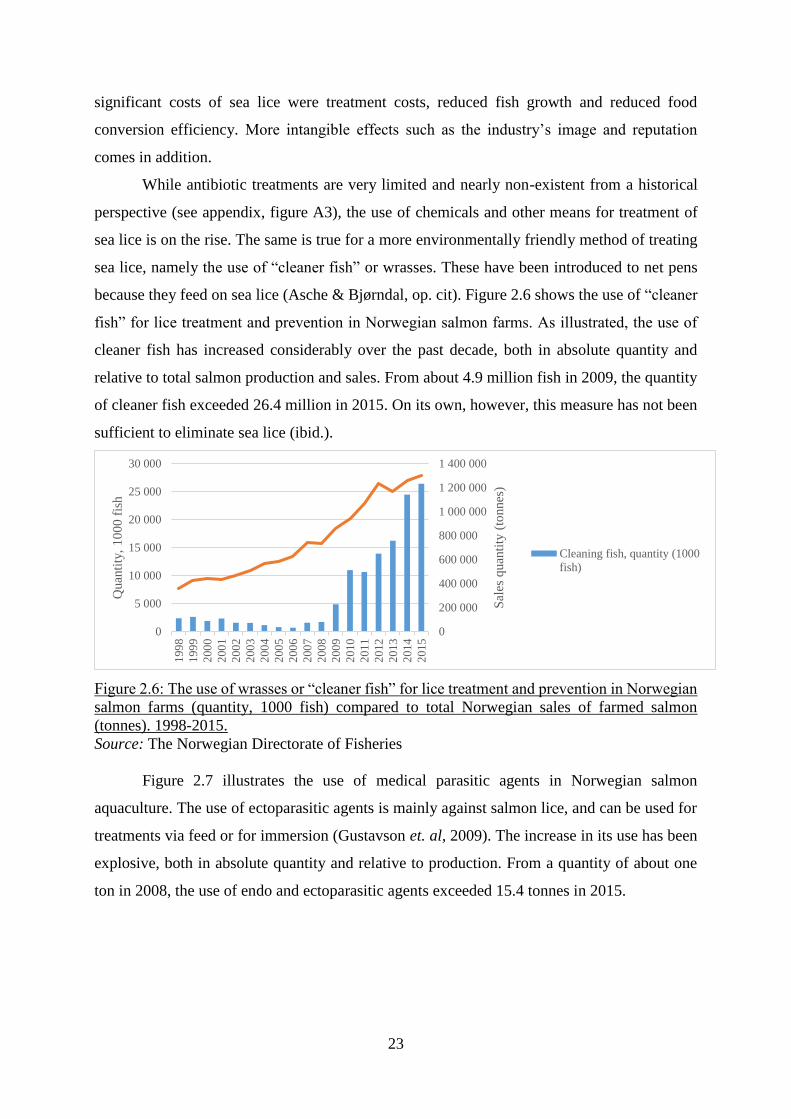
While antibiotic treatments are very limited and nearly non-existent from a historical

perspective (see appendix, figure A3), the use of chemicals and other means for treatment of

sea lice is on the rise. The same is true for a more environmentally friendly method of treating

sea lice, namely the use of “cleaner fish” or wrasses. These have been introduced to net pens

because they feed on sea lice (Asche & Bjørndal, op. cit). Figure 2.6 shows the use of “cleaner

fish” for lice treatment and prevention in Norwegian salmon farms. As illustrated, the use of

cleaner fish has increased considerably over the past decade, both in absolute quantity and

relative to total salmon production and sales. From about 4.9 million fish in 2009, the quantity

of cleaner fish exceeded 26.4 million in 2015. On its own, however, this measure has not been

sufficient to eliminate sea lice (ibid.).

Figure 2.6: The use of wrasses or “cleaner fish” for lice treatment and prevention in Norwegian

salmon farms (quantity, 1000 fish) compared to total Norwegian sales of farmed salmon

(tonnes). 1998-2015.


Figure 2.7 illustrates the use of medical parasitic agents in Norwegian salmon

aquaculture. The use of ectoparasitic agents is mainly against salmon lice, and can be used for

treatments via feed or for immersion (Gustavson et. al, 2009). The increase in its use has been

explosive, both in absolute quantity and relative to production. From a quantity of about one

ton in 2008, the use of endo and ectoparasitic agents exceeded 15.4 tonnes in 2015.

0

200 000

400 000

600 000

800 000

1 000 000

1 200 000

1 400 000

0

5 000

10 000

15 000

20 000

25 000

30 000

199

8

199

9

200

0

200

1

200

2

200

3

200

4

200

5

200

6

200

7

200

8

200

9

201

0

201

1

201

2

201

3

201

4

201

5

Sal

es q

uan

tity

(to

nnes

)

Quan

tity

, 1

00

0 f

ish

Cleaning fish, quantity (1000

fish)

24

Figure 2.7: The use of endo and ectoparasitic agents in Norwegian salmon aquaculture in

quantity (tonnes) compared to total Norwegian sales of farmed salmon (tonnes). 1996-2015.

Source: Norwegian Institute of Public Health.

Another chemical used in the treatment of sea lice is hydrogen peroxide. Reliance on

medical delousing resulted in widespread resistance amongst salmon lice. In attempt to combat

resistant salmon lice, hydrogen peroxide (H2O2) became increasingly used in salmon immersion

(lice bath) treatments (Helgesen et. al, 2017). Its use increased tremendously in absolute as well

as in relative quantity, starting from 2009. From a quantity of 308 tonnes in 2009 (zero in 2008),

the use of hydrogen peroxide exceeded 43 thousand tonnes in 2015.

Problems related to resistance reached new levels in 2016, with observations of

accidents under treatments and lice related fish damages at many sites (Hjeltnes et al. 2017). In

the same year, the number of medical treatments declined by 41%, while the number of

mechanical treatments increased six-fold (ibid.). An important explanation for the repeated

change in treatment form is the development of resistance against the medical and chemical

treatments used (ibid.). Meanwhile, reported incidences of substantial mortalities following lice

treatments are substantially higher for mechanical than medical lice treatments (93% versus

65% of respondents, respectively) (ibid.).

In 2016, 1,122 salmon and trout permissions in Norway14 were distributed over 566

active locations with a total number of mechanical and medical lice treatments of 3,662, or on

average 6.5 per location. In addition, 2702 locations released cleaner fish into net-pens.

Whether the entire location or only part of it is treated may vary on a case by case basis. It

should be kept in mind that the incidence of lice varies from year to year and it also varies along

the coast. In 2016, two counties in Western Norway (Hordaland and Sogn and Fjordane) and

Middle Norway (Nord- and Sør Trøndelag) were relatively most affected. It is also noticeable

14 Source: The Norwegian Directorate of Fisheries.

0

200 000

400 000

600 000

800 000

1 000 000

1 200 000

1 400 000

0

2

4

6

8

10

12

14

16

18

199

61

99

71

99

81

99

92

00

02

00

12

00

22

00

32

00

42

00

52

00

62

00

72

00

82

00

92

01

02

01

12

01

22

01

32

01

42

01

5

Sal

es q

uan

tity

(to

nnes

)

Dru

gs

quan

tity

(to

nnes

)

Endo and ectoparasitic agents

Sales quantity (tonnes)

25

that the two northernmost counties, Finnmark and Troms and Nordland, are much less affected,

presumably due to lower water temperatures.

While data on lice treatments are presented mostly for Norway, salmon lice are a

substantial concern in all salmon producing countries (Abolofia et al. 2017).

2.3.4 Smolt Production

Smolts are essential inputs to salmon aquaculture (Sandvold & Tveterås, 2014)15. In terms of

costs, smolt is the most important input factor in salmon farming after feed and is also

considered a major determinant of loss and mortality throughout the life cycle (Sandvold &

Tveterås 2014; State Secretary Roy Angelvik16). Figure 2.8 provides an overview of important

developments in smolt production quantity and real cost of production during the period 1988–

2010. From a quantity of 57 million smolts in 1988, Norwegian hatcheries produced 280 million

in 2010 (nearly 333 million smolts in 2015). The increased production over time has been

accompanied by a substantial reduction in the unit production cost and real sales price. In 1988,

the real production costs were around NOK 16 per unit, while in 2005 it reached its lowest

reported level at less than NOK 6 before levelling off17.

Figure 2.8: Total production of smolt and the associated prices and costs in the Norwegian

salmon industry in the period of 1988–2010. Data from the Norwegian Directorate of Fisheries

(1988–2010).

Source: Sandvold, H.N. & Tveterås, R. (2014).

15 Juvenile production is land based fresh water farming, and includes production of both fry and smolt. The fish

is called fry from its hatched at the age of 4-6 weeks and until it reaches the smoltification stage at the age of 8-14

months. Fry is sold to other hatcheries for further growth in fresh water. Smolt is sold to grow-out farms for further

growth in salt water. Hence, smolt is the main product of interest for the hatcheries. 16 Presentation at «Smolt production of the future», a conference, Sunndalsøra, Norway, October 25 th, 2016. 17 For a break-down of nominal production cost, see Appendix, table A1.

26

The real sales price per smolt also experienced a clear downward trend during the

industry’s first decades, contributing to lower cost of production for the grow-out plants. In

1988, the sales price was around NOK 26 per unit, while by 2010 it had decreased to NOK 9.

Like for the salmon grow-out farms, there is a close relationship between the trend in production

cost and price, indicating a competitive industry (Sandvold & Tveterås, 2014). Looking at the

more recent years (i.e., including some years after 2010), cost of production has been rising in

nominal terms, while operating margins seem to have been under pressure (figure 2.9)18.

Figure 2.9: Development in average cost of production per smolt and average operating margin

in Norway. 2008-2015. NOK (nominal) and margin %.

Source: The Norwegian Directorate of fisheries

Another trend in the same period has been increasing investments (figure 2.10). It may

be noted that since 2011, restrictions in terms of production capacity in number of smolts were

abolished. Instead, the capacity is now limited by restrictions on water consumption (set by

NVE, the Norwegian Water Resources and Energy Directorate) and restrictions on waste

quantity (set by the chancellor). A former restriction stating the maximum permitted smolt

weight was also abolished in 2016 (The Norwegian Government 2015b; 2016).

18 For the development and composition of cost of production per smolt in Norway, see appendix, tables A1 and

A2. When it comes to possible changes in the product sold – such as for instance smolt size – this is not discernable

from the statistics.

27

Figure 2.10: Development in investments in the Norwegian salmon smolt and fry industry.

Nominal NOK, 1994-2015.


From industry statistics, only average figures are available on cost of production and

prices. However, in terms of operating margin it is possible to look a bit more into variations

within the industry. It can be noted that although the performance in operating margins seem to

have been converging lately, they are not uniform across the Norwegian industry – although

this may very well be explained by prices as well as costs19. Nevertheless, apart from the county

of Møre and Romsdal which showed a terrible development in average operating margins over

the three years from 2013-15, average operating margins varied between 10.3-15.2% among

geographical regions (Table 2.2; figure 2.11). Compared to the historical variation, that range

is rather narrow.

Figure 2.11: Average operating margin for Norwegian smolt producing firms. Average numbers

per county and for the industry as a whole. Operating margin in percent, 2008-2015.


19 Equivalent statistics on price and cost between regions have not been obtained. Moreover, the differences might

be just as large within regions as between.

28

Table 2.2: Average operating margin for Norwegian smolt producing firms. Average numbers

per county and for the industry as a whole. Operating margin in percent, 2008-2015.

Operating margin 2008 2009 2010 2011 2012 2013 2014 2015

Norwegian industry average 19,5 16,2 15,8 16,4 15,0 10,0 13,3 10,3

Finnmark & Troms 10,9 26,4 16,2 15,2 12,3 12,6 8,4 12,2

Nordland 24,6 13,0 13,5 18,4 15,1 16,6 17,9 13,0

Trøndelag 15,0 14,0 20,3 19,9 20,1 17,1 19,2 11,9

Møre & Romsdal 21,2 17,8 13,7 12,0 14,3 -2,8 -4,8 -7,5

Sogn & Fjordane 12,6 13,6 13,9 11,5 10,5 9,4 12,1 10,3

Hordaland 15,9 17,7 16,4 18,0 12,8 17,9 15,4 15,2

Rogaland, Agder and Telemark 28,6 26,9 29,8 15,6 25,5 18,0 9,2 14,5

Over the years, plant size in smolt production has increased. Figure 2.9 shows the

development in the number of fish released compared to the number of companies and

permissions from 1994-2015. While the industry’s output increased considerably – here

represented by the release of smolt to sea – the number of smolt producing companies

decreased. Thus, an intensification of the industry has taken place also in the case of smolt

production.

Figure 2.12: The number of companies, permissions and release of fish in Norwegian salmon

and trout aquaculture production. 1994-2015.


In terms of production restrictions, the smolt production permissions vary substantially

in size (Sandvold & Tveterås, 2014). Originally, the licenses were given in terms of the

maximum number of smolts to be produced each year, but recently one has been moving

towards a system that more explicitly addresses environmental issues (ibid.). With respect to

former restrictions, concerns were raised that certain regulation could have the unintended

consequence of limiting innovation, flexibility and development of new production models

29

(Asche et al. 2014). As such, new licenses are issued in terms of maximum withdrawal of

freshwater and maximum discharge of wastewater.

In juvenile production, the technology has changed rapidly over the past decades – with

improvements in breeding, fish health, feed and equipment (Sandvold & Tveterås, 2014). Many

of the largest innovations in salmon farming have first taken place in smolt production, for

example artificial light, water purification system and vaccines. Improved fish health through

vaccination has been among the most important measures to prevent spread of diseases.

Production technology and production practices vary between plants, and the industry

is more heterogeneous than in earlier years (Sandvold & Tveterås, 2014). In the 1970s, the

technology was more or less similar for all plants (ibid.). All the hatcheries operated “flow-

through-systems” with no reuse of inlet water and little cleaning of the outlet water (ibid).

Recirculation Aquaculture Systems (RAS) technology, which is a closed containment water

purification technology with drastically lower water consumption, was first introduced in

Norway in 2006 and is now used by many of the new plants (ibid.). Together with regulatory

changes, water recirculation has opened new opportunities for land based production of larger

smolts. As noted, a long held maximum limit on smolt size of 250 grams has been eliminated,

following the introduction of a new regulation of land-based aquaculture (starting from June

1st, 2016)20.

Introduction of RAS and water purification systems may also contribute towards a more

environmental sustainable production (Sandvold & Tveterås, 2014). New hatcheries today have

close to zero escapes, low water consumption and effective cleaning of the outlet-water.

Improved control over the production process reduce risk when it comes to accidents, escapees

and diseases and can potentially offer a higher degree of flexibility and utilisation of capacity

for both the land based smolt production and the grow-out farms (ibid.).

2.3.5 Regulation of the salmon aquaculture industry in Norway

All salmon producing countries regulate their industries. Regulations are focused on ensuring

that environmental standards are met and coastlines appropriately protected (Asche & Bjørndal,

op.cit, 34). All countries require an environmental impact assessment, although specific

standards differ. As the regulatory requirements vary, so does industry structure and

competitiveness (ibid).

20 From 2012 and up until then, smolts exceeding 250 g could only be produced with a special exemption from the

Norwegian Fisheries Directorate, with application procedures required.

30

Production licenses are the most important tool used in controlling the production

capacity in the Norwegian industry (Asche et al. 2014). The salmon industry in Norway has

been regulated since salmon farming became commercialised, and the first set of regulations

was introduced in 1973 (Asche & Bjørndal, op.cit, 34). Operating as a preliminary law, it

registered the number of firms (licences) that operated in the country, as well as the production

per firm (licence) (Stikholmen, 2010; Bjørndal, 1987). In the beginning, the permission system

was very liberal and functioned more in terms of a registry. Up until 1977 almost all

applications were permitted (Bjørndal, 1987). For a short look at some historical developments

in regulations and the associated changes to industry structure, see appendix, note A2.

In 2005, today’s maximum total biomass (MTB) regulation was introduced (Asche &

Bjørndal, op.cit). As indicated by the name, the MTB sets the maximum biomass allowed in

sea per permission at any time. Initially, it was set to 780 tonnes21 per permission (ibid) and this

quota remains the same today. The MTB system operates at two levels: the company level,

where the maximum biomass is determined by the company’s number of permissions (at a

quantity of 780 tonnes per permission) and at the level of a location. The latter is determined at

an individual basis with respect to the location’s ecological and environmental capacity.

Chapter VI will revert to the discussion about the MTB regulation system in a more practical

approach to consider its implications on production planning.

During most of the Norwegian salmon industry’s history, licenses have been awarded

for free, although often with substantial regional policy considerations (Asche & Bjørndal,

op.cit, 35). However, in 2002 the government introduced a fee of NOK 5 million per

license(except for the most northern county, Finnmark, where the fee was NOK 4 million). In

2008, the fee was increased to NOK 8 million (NOK 5 million for Finnmark) (ibid.). Limits on

the maximum share of total production licenses that can be owned by a single firm existed up

until 2015 to prevent too much concentration. Until November 2015, an industry player had to

apply for approval from the Government to be in control of more than 15% of the total permitted

biomass in Norway22. The regulations were deemed in conflict with the European Economic

Area (EEA) agreement by the European Free Trade Association (EFTA) court in 2010 (EFTA

2012)23. As a consequence, the regulation of ownership was proposed removed in September

2014, a decision first implemented in November 2015. Requirements about product processing

21 Except for a preferential treatment of the two northern counties Troms and Finnmark, with a maximum allowed

biomass of 945 tonnes per licence (The Norwegian Directorate of Fisheries, 2016). 22 Such approval could be given if specific terms regarding the applicants R&D-activity, fish processing and

apprenticeships in coastal regions were upheld (Marine Harvest, 2016). 23 Following complaints from Marine Harvest, the largest salmon aquaculture firm.

31

with increasing license ownership concentration were also abolished in the same year (Intrafish,

2017a). However, it still applies that no industrial player can control more than 50% of the total

biomass in any of the regions of the Directorate of Fisheries (Marine Harvest, op. cit).

As of today (2017), the main objective of the regulation is to ensure environmental

sustainability (e.g. Asche et al. 2014, The Norwegian Government, 2017). Yet, the criteria for

granting new permissions have been varying from one round of license grants to another –

including considerations such as fish processing, lice count, company structure and production

technologies. New permissions have been awarded with uneven and unforeseen intervals,

making the growth in production capacity uncertain and unpredictable (ibid). Since 2002, all

allocation rounds have upheld various preferences with respect to the organisation of the

industry – including policy criteria related to processing, company structure, research and

development and the technology applied in production (Asche et al. 2014). For instance, a

recent allocation in 2013-14 involved both an open auction of permissions (with licenses to be

granted to the highest bids) as well as a number of permissions reserved for companies which

fulfilled certain policy criteria (ibid). The group of companies which fulfilled the relevant

criteria were granted permissions at a price of NOK 10 million. Meanwhile, among ordinary

bidders in the same round (not conforming to any criteria), 15 licenses were traded with prices

ranging from NOK 55 million to 66 million (with the highest bid not to be granted any license

at NOK 55 million) (ibid.).

Sea lice infection on salmon farms has been regulated since 1997 to reduce the harmful

effects of lice on farmed and wild fish (Abolofia et al., 2017). Regulations set thresholds for

the maximum mean number of sea lice per fish (lice count) and a compulsory reporting system

is operated. From 2000 to 2013 the legal lice infection thresholds, enforced by the Norwegian

Food Safety Authority (NFSA), was set to 0.5 adult female lice per fish or three lice per fish of

other mobile stages (i.e., adult males or pre-adult mobiles) in the period Jan. 1st – Aug. 31st; and

one adult female or five other mobile ones per fish in the period Sep. 1st – Dec. 31st (ibid.). If

thresholds are exceeded it is mandatory for the farmer to medically treat or slaughter their fish

within 2 weeks (ibid.).

Recently, a new growth system to be implemented October 1st, 2017 has been presented

for the Norwegian salmon aquaculture industry (The Norwegian Government, 2017). The

intention is to ensure sustainable growth of the industry, with future growth to be granted based

on sustainability indicators, currently sea lice (Marine Harvest, 2016). Labelled as the “traffic

light system”, the regulatory system divides the country into 13 production areas and assigns

the codes green, yellow or red to each area depending on their performance on predefined

32

environmental criteria set by the government. Based on assigned codes, each production area

may be allowed to increase its production (green light), freeze its production (yellow light) or

required to reduce production (red light). If the environmental criteria are satisfied within a

region, the region can grow by a maximum of 6% for every two-year period – a quantity which

is to be distributed between existing and new licenses (The Norwegian Government, 2015a;

Marine Harvest 2016; Intrafish, 2017b). Thus, the producers shall be encouraged to take

responsibility for the area in which they produce, and good practices and routines will be

rewarded with growth (Nrk.no, 2017). The division into 13 areas is based on scientific research

by the Norwegian Institute of Marine Research (IMR), undertaken to model ocean currents and

the spread of sea lice along the cost. Using cluster analysis, a statistical technique, they

separated the coast line into areas in which sea lice tended to spread within but not between

(IMR, 2015).

With respect to land based production in Norway, a recent change to industry

regulations has served to substantially lowering barriers to entry in land based salmon

aquaculture, while simultaneously eliminating restrictions on the production of smolts. Per

June 1st, 2016, the Norwegian Directorate of fisheries set into force a set of new rules for the

issuing of permissions to establish land based aquaculture operations in Norway (The

Norwegian Government, 2016; the Norwegian Directorate of fisheries, 2016). Most

importantly, it was opened for operating licenses to be issued continuously and without

proceeds (apart from a processing fee, which remains). The application procedure is

decentralised to the county level, where the relevant county processes applications and issues

licenses to operate continuously. The changes were implemented based on recommendations

made in the previously cited report “Salmon on land” by Holm et al. (2015), where a working

group was given the mandate to explore the status of land based aquaculture and to recommend

any changes needed to lower barriers to this type of aquaculture operations – if recommendable.

Following the recommendations, the described changes were implemented, while former

restrictions on smolt weight were also abolished (the Norwegian law of aquaculture, Chapter 5

§55).

2.4. Land-based aquaculture

As illustrated in this chapter, a combination of high salmon prices, increasing production cost

in traditional sea pen farming and encouragements from the government to innovate and explore

new technologies have all contributed to drive forward the development in land based

aquaculture and other technologies (which will not be discussed here). As the costs and risks

33

of keeping fish in the sea have increased in Norway, adaptations to production include keeping

the salmon on land for longer. As shall be described later, other countries are moving in the

same direction. Not only is traditional salmon production getting more expensive, but land

based competitors are attracted by the opportunity to avoid license investments and potentially

eliminate transportation costs by locating closer to major markets (savings of as much as NOK

13-18 per kg by air freight to the important Asian and US markets, by some estimates – see e.g.

DNB Markets 2017; ilaks.no, 2016a).

2.5.1 Land-based aquaculture technology

Closed containment technologies have become a major focus of aquaculture research and

development (House of Commons Canada, 2013). Closed containment systems (CCS) describe

aquaculture facilities on land or in the sea that have a separating barrier between the fish and

the environment around the facility. Land-based aquaculture systems is one of these

technologies, which has come into focus as a means of protecting both farmed and wild species

from issues such as genetic interaction and disease.

The (modern) history of land based aquaculture technology began in the mid-late 19th

century, when fish hatcheries and fish culture facilities originated in Japan, Canada, Norway

and the United States to restock declining commercial and recreational fish stocks (International

Salmon Farmers Association, 2016). Traditional land-based aquaculture systems have been

based on a flow-through technology, pumping water into the tanks and using it only once (Holm

et al, 2015). However, the past 20-35 years have seen a considerable development within

recirculation technology (Holm et. al, 2015; Liu et al, 2016). First trialed for carp in Japan in

the 1950s, recirculation aquaculture systems (RAS) underwent a revival in the 1980s as

technological advances made them more viable (Intrafish, 2015). RAS, where 95-99% of the

water is reused, have become increasingly popular ever since (Holm et. al, 2015).

Compared to the earlier technology, the RAS systems require substantially less water,

have lower costs of pumping and energy, are assumed to provide better control with the

production environment and new solutions for reduction of waste disposal to the sea. According

to industry sources24, the major benefit of using recirculation technology is that it provides

stable, environmentally controlled conditions for rearing fish in terms of temperature, oxygen

content, pH and overall water quality. This in turn promotes greater fish health, better quality,

superior growth rates, improved feed conversion ratios, reduced disease outbreaks and lower

24 Jacob Bergnballe, business director of land based aquaculture for Akva Group, one of the world’s largest

providers of RAS systems (Intrafish 2015).

34

use of therapeutants (ibid.). Supporters of the technology envision environmental gains through

eliminating interactions with wild species, improved fish health, better growth rates and zero

emissions through the reuse of energy, water and waste (Liu et al. 2016). Moreover, the

development of RAS internationally has made possible the establishment of land-based

aquaculture of fish for human consumption on locations formerly not considered, including the

opportunity of locating production closer to major markets (ibid.).

Currently, advanced reuse systems represent only 4.5% of the total aquaculture market

(Basu, 2015). RAS systems currently account for 6 percent of total production in China and 12

percent in both the United States and Europe (ibid). By 2030, Basu (2015) predict that RAS

will produce over 40% of the total aquaculture output. According this study, Europe is poised

to become a leader in water recirculation systems.

Besides the optimistic predictions stands a substantial global track record of company

failures in using RAS, for reasons including economic viability, biological challenges and

difficulty of operating the systems at commercial scale (Intrafish 2015). When it comes to

technology diffusion at a large scale, many uncertainties remain about cost competitiveness,

regulatory support and access to financing and resources, including coastal land, water and

energy (International Salmon Farmers Association, 2016). RAS technology has come a long

way over the past 30 years but is still at an early stage of development for large-scale

commercial grow-out, particularly of marine species (Intrafish, 2015)25. Nevertheless, it is

expected that the economic barrier to using RAS gradually should be lowered as technology

improves and economies of scale are realised (Intrafish 2015; Iversen et. al, 2013; Liu et. al,

2016).

In hatchery and fry systems, RAS technology is already being applied all over the world

(Intrafish, 2015). Opportunities to give fish the best conditions when they are young result in

healthy juveniles that experience fewer problems during grow-out. Although new and

unfamiliar challenges may show up in relation to new technology, it is believed by many that

RAS offers the potential to exercise considerable control over the aquaculture environment so

that optimal growth and fish health conditions may eventually be achieved and sustained in

such systems. With greater control over critical elements of the production process, this could

25 In the seabass and seabream sector, there is increasing use of recirculation systems for grow-out and it has long

been common for trout to be farmed from egg to harvest using the system. In the Middle East, projects are being

developed for seabream, grouper and barramundi. However, for larger-scale production of tilapia, which is

particularly relevant in China, systems need to become larger and cheaper to become attractive and profitable

(Intrafish, 2015). High-value species such as shrimp are also targeted for production in RAS, after seeing

substantial sustainability and disease issues in pond based aquaculture (East Asia Global Alliance, 2014)

35

in turn reduce mortality while shortening the production time in sea, including for salmon

(ibid.).

2.5.2 Land-based salmon aquaculture

With ongoing technological improvements, freshwater aquaculture of salmon from eggs to

harvestable sizes of 4–5 kg in land-based systems (particularly RAS) is increasingly receiving

attention from the industry, investors, regulators, academics and the press, evaluating its

potential as a viable production technology (Liu et. al, 2016). The control and flexibility offered

by RAS may offer certain advantages over salmon operations in open sea-pen systems, which

require expensive licenses, are negatively impacted by sea lice, dependent on access to suitable

coastal sites and typically has a relatively long transport distance (and high transport cost) to

supply important markets (ibid).

2.5.2.1 The state of land-based salmon aquaculture

In salmon aquaculture, the production of fish for human consumption is as noted carried out

mostly in sea, while the first phase of fingerling production, typically up to a size of

approximately 100 grams, takes place on land. Smolt producers are increasingly extending the

land-based production phase, allowing for increased smolt size before the transfer to the marine

environment (ISFA, 2016). For this purpose, the salmon aquaculture industry increasingly

invests in technological improvements to land-based salmon farming systems and RAS,

recognising that it may have a potentially valuable role to play for the future salmon production

(ibid.). For instance, Marine Harvest reports that the majority of their investments currently go

into the development of its freshwater sites for smolt production (Intrafish, 2016a). Bakkafrost,

a Faroese salmon producer, is increasing investments in hatcheries to reach its long-term goal

to raise the smolt size to 400-500 grams per fish by 2019 (Intrafish 2016b). Grieg, another

salmon producing firm, has presented their new strategy of reducing the salmon production

time from 24 months to 18 months by releasing bigger and stronger fish to sea-pens and thereby

reducing risk and exposure time in sea (Intrafish 2016c).

Because of the control of important parametres such as temperature in land based

facilities, the length of a production cycle can be considerably shorter when producting larger

smolts before release to sea. A prolonging of the initial land based phase leads not only to an

overall reduction in production time, but also a much shorter exposure time in sea. This gives

rise to the benefits of lower production risk, less exposure to sea lice sea and lice treatments

and shorter periods between fallowing of production sites. Parasites and diseases will have less

time to accumulate before a site is emptied, and infected fish may be harvested instead of

36

receiving treatment. Moreover, the long production cycle in traditional production means that

the fish are exposed twice either to the unfavourable periods of the lowest temperatures and the

slowest growth or to the unfavourable periods with the highest risk of sea lice infection. By

extending the land based phase before release to sea, these issues are addressed, while

production risks may presumably be shifted to some extent from factors outside of the farmers

control to more manageable and controllable production risks.

As traditional farmers are extending the production phase on land, similar production

modes may also be adopted in unconventional areas. Notably, in South Korea the country’s first

salmon has been delivered to market, using post smolt (200-400g) combined with sea based

grow-out (Korea Herald, 2016). While the producer aimed at supplying 400 tonnes by year-end

2016, it hoped to increase its production to 10-20,000 tonnes by 2020 (ibid.).

DNB Markets quantify the growing number of RAS facilities for smolt in Norway, as

producers recognise the advantages of reducing time fish spend in the sea. The number of RAS

facilities increased to a total of 90 in 2016, up from around 20 three years earlier (DNB Markets,

2017). Equipment providers report activity higher than ever with large backlogs on new projects

(ibid.). With an increasing number of RAS facilities, it follows that investments in new

technology have been substantial (DNB Markets, 2017). Technology improvements following

smolt producers demand for larger facilities for larger smolts may in turn have contributed to

the feasibility of extending land based aquaculture further towards full land based grow-out

(ibid.). As illustrated in chapter II (figure 2.10), investment in smolt and fry production rose

considerably from 2004 to 2015.

Land-based farming of salmon for human consumption still has a minimal scope

globally. In 2007, at least 40 trials with capital investment exceeding $283 million had been

conducted on for production of Atlantic salmon at harvestable sizes around the world (Canadian

Science Advisory Secretariat, 2008). Yet, as of 2016, only one Danish facility was close to

reaching an annual production level near 1,000 tonnes (<700), while the minimum efficient

scale is probably quite a bit higher than that. As the former sections revealed, this has not

stopped interest in land based salmon aquaculture facilities from rising. On the contrary, a

number of commercial land-based farms are being planned, built and set into operation in

Europe, North America, China, and Norway (Liu et al, 2016). Billund Aquaculture Service, a

leading supplier of land based aquaculture technology, report “huge request” for land based

salmon and trout grow-out in RAS (Olsen, 2017). The company reports making at least one

37

quote for projects on a weekly basis, with requests from at least 15 countries including from

Europe, Asia, North America and Africa26.

A look at planned land based projects suggest that the collective impact on the industry

supply could be substantial if the expansions are realised. DNB Markets (2017) calculated that

the planned salmon production capacity from 20+ identified land based projects amount to 150

thousand tonnes in early 2020, potentially making land based salmon among the major salmon

supply sources if the plans are successfully carried out27. Among the projects identified by

DNB, the majority is based on RAS technology and originate in regions familiar with salmon

production; the Nordics, Canada and the US, presumably with links to existing knowledge hubs.

Nofima, a Norwegian research institute at the forefront of land based aquaculture trials

and biological research, carries out full cycle grow-out and has undertaken both biological,

economic and market related studies of land based salmon and post smolt. The researchers

emphasise the potential of RAS in addressing industry challenges such as escapees, disease and

sea lice (Nofima, n/d).

Trials and experiments with full grow-out of Atlantic salmon on land continue around

the world at various rates of expansion, and thus far with various degrees of success. This may

be due to a number of factors, including the level of understanding with respect to the biological

needs in land based systems, new challenges including bacteria and water management,

differences in regulatory support, cost and market conditions, access to financing and other

resources including land, water, energy, knowledge and competent labour and other inputs.

Nevertheless, as research progress and the few companies in operation continue to address and

resolve biological and other challenges while newcomers continuously appear, the learning

curve may well be steep in the land based production sector for the time to come.

2.5.2.2 The economics of land-based salmon aquaculture

A few studies have performed comparative economic analyses of closed-containment options

including land-based technologies, exploring their economic feasibility in relation to the

conventional production approach. In the following, a brief review is presented of some of the

studies that have undertaken economic comparisons of land-based production and traditional

26 Billund Aquaculture: Global Trends in Commercial Salmonid RAS. Presentation at TEKSET, a conference,

February 15, 2017 in Trondheim, Norway. 27 After Norway and Chile, the UK and North America (Canada) constitute the major supply sources, each of the

latter two with respective production of around 150 thousand tonnes annually in 2015 and 2016 (Marine Harvest,

2016). It should be emphasised that out of the 150 thousand tonnes planned, three major projects (each of 30-40

thousand tonnes) constitute around 100 thousand tonnes of the identified total production (DNB Markets, 2017).

The projection does not count potential increases from combined production modes (post smolt).

38

sea-pen operations. Their findings with respect to initial investment is first provided, followed

by comparative costs of production. A notable challenge in trying to compare and assess the

findings is that each study is carried out under various assumptions, for a particular production

capacity, with varying equipment and components and in a specific context. Moreover, it is

important to note that in common with the current study, all are engineering studies, meaning

that estimates and data are highly uncertain. To the best of our knowledge, no analysis based

on actual data from large, full-scale facilities exist (simply because such operations at has yet

to be established).

The findings of the studies broadly align with respect to assessments of risks –

concluding that land-based production involves a larger degree of uncertainty (King et al. 2016;

Iversen et al, 2013; Boulet et al, 2010). King et al. (2016) found that the financial risk, as shown

by the level of uncertainty of the result, was greater for land-based RAS production technology

than for three alternative production approaches analysed. This assessment is consistent with

the findings of other analyses (e.g. Boulet et al, 2010; Iversen et al, 2013 and Liu et al, 2016).

The study by King et al. (2016) was conducted with a focus on Tasmanian aquaculture

operations, where each of the production scenarios were developed with an annual capacity of

6,000 tonnes HOG production. Their findings indicated that the initial capital investment

required for land-based RAS was approximately two times greater than the equivalent

investment for inshore sea-pen production.

Boulet et al. (2010) analysed and compared the economic feasibility of five production

approaches, including conventional net-pens, in the context of the Canadian industry within the

operating environment in British Columbia. Assuming an annual production of 2,500 tonnes,

they estimated initial investment requirements in RAS more than four times the requirements

for inshore sea-pens.

Liu et al. (2016) modelled production facilities of 3,300 tonnes for sea-pens and RAS,

respectively, and estimated capital investments of approximately $30 million for sea-pens and

approximately $54 million for the RAS system, i.e., less than two times as much (a difference

of 80%). Their data was based on Norwegian salmon farmers’ operations in the sea-pen

scenario, while the land-based scenario was based on data developed by The Conservation

Fund’s Freshwater Institute grow out trials of Atlantic salmon in RAS.

Iversen et al. (2013) compared five alternative production approaches in a Norwegian

context. Investments in the base case, inshore net-pens, was estimated at 220 NOK per m3 of

production volume – based on actual numbers from a group of Norwegian firms with annual

production of 8,800 tonnes per company. The RAS facility assumed a production of 3,300

39

tonnes per annum and investments of 10,000 NOK per m3 of production. Production

density/productivity for the two alternatives were respectively 30 kg/m3 in net-pens and 180 kg

per m3 in RAS.

With regard to findings about cost of production, King et al. (2016) emphasised the high

uncertainty in modelling cost of production in RAS. Nevertheless, using statistical simulations

(Monte Carlo simulation), they estimated that around 90% of the simulated RAS grow-out

would have a superior cost of production compared to Tasmanian south-east inshore sea pen

production. The steady state cost of production was budgeted to AU$ 5.12 per kg in RAS

compared to AU$ 5.65 in sea pens, which is a difference of 9.4% to the advantage of RAS.

According to Liu et al. (2016), the total operating costs for the two systems were

relatively similar, with RAS only 10% higher than the sea-pen system. Without interest and

depreciation, the two production systems seemed to have an almost equal operating cost, 4.30

US$/kg for sea pens and 4.37 US$/kg for RAS. Conversely, Boulet et al. (2010) estimated cost

of production to be higher in RAS than in sea pens, with a disadvantage of 18%. Iversen et al.

arrived at the same conclusion, estimating a cost disadvantage in RAS of 27.6%. On the other

hand, Rosten et. al reported somewhat lower production costs in RAS, where total production

costs were estimated to $ 14 million in sea-pens (corresponding to $ 4.24 per kg) and $ 13.1

million in RAS (corresponding to $ 3.97 per kg) for production of 3,300 tonnes (King et al.

2016). In this case, the estimated cost advantage in favor of RAS amounts to 6.6%. A recent

report by DNB Markets (2017) estimated that the land based cost of production is approaching

that of conventional Norwegian sea pens, estimating cost of production in land based salmon

farming to NOK 37 per kg, with the corresponding number for sea based production in 2016

being NOK 36 per kg.

As the discussion illustrates, results and findings vary widely. Apart from the fact that

actual data cannot be obtained, this is likely to be a result of differences in assumptions,

operational design, time period of the studies as well as the context (geographical location),

involving actual differences in the same concepts depending on location. It is noted that

comparability between studies is complicated due to differences in scale, country and regulatory

environment, costs (e.g. energy costs between countries), difference in treatment of costs and

investment (notably the value of sea based licenses, which seems disregarded in many studies),

biological assumptions, whether the analysis includes harvesting and/or primary processing and

more.

40

2.5 Summary

It is clear from this review that while interest in land based salmon aquaculture is increasing,

views on its viability and how it is likely to unfold diverge. Moreover, academic literature on

the economics of land based aquaculture is rather limited. Indications suggest that both the cost

of production and necessary investments are converging somewhat between traditional and land

based aquaculture, but the evidence remains scarce, and estimates rely heavily on assumptions.

Production cost estimates for land-based facilities are engineering studies rather than data

based, as such data in practice still does not exist. Without empirical data, it follows that the

uncertainty is large. Nevertheless, with high salmon prices, binding regulations and limited

supply growth, increasing costs and biological challenges in traditional farming, the risk-reward

is looking attractive enough for investments in land based salmon aquaculture already to have

started to take off.

Meanwhile, traditional farmers are increasingly interested in deploying the benefits of

land based technology in combination with sea based net pens and their “natural competitive

advantage”. To direct well-informed expansion and to better understand the potential impacts

of new technology on the industry as we know it, more knowledge is needed about the

economics of land based aquaculture. This study will contribute to the discussion by examining

the economic competitiveness of land based salmon production models in terms of cost of

production and potential profitability of investments (NPV).

We now turn to a discussion of the methodology to be applied in the analyses.

Methodology is presented in chapter III.

41

III. METHOD

3.1 Introduction

The analyses to be undertaken in this study aim at investigating investments in land-based

farming of salmon. Extending knowledge about the economic competitiveness of new

technology is of relevance for strategic decision making by companies and policy makers, as

increasing amounts of investment is seen to be flowing into the construction of land-based

salmon farms globally. Two main methods are applied: investment analysis (net present value

(NPV) and internal rate of return (IRR)) and steady state cost analysis. Both to provide

fundamental insights into the questions of economic returns and profitability.

The study analyses two main scenarios: 1) full land based production of salmon up to a

harvestable size of about 5 kilograms and 2) “post smolt” – an extension of the initial land-

based smolt phase. The post smolt scenario looks at release of post smolts to sea at 400 grams

and 600 grams, respectively, instead of the traditional release at a size of about 100 grams. The

alternatives are compared to the traditional production model.

Because of the long production cycle for salmon to grow from hatching of eggs to a

harvestable size, it may take several years from the development of a farm until it reaches full

production (Asche & Bjørndal, 2011). To analyse cost of production, a steady state situation is

assumed, meaning that the farm is fully operational (ibid.). This provides an important

indication about the price the firm will need to fetch in order to be financially viable over time

(ibid.). This complements the NPV analysis by providing more interpretable information about

the cost competitiveness among alternative production modes and a basis to assess cost of

production in relation to market prices.

The scenarios are analysed and evaluated in relation to the objective of maximising

efficient use of society’s resources. That is, it seeks to evaluate the profitability of the alternative

production modes without consideration of taxes and subsidies, which from a private

perspective might affect or distort relative attractiveness. From the public’s perspective28, these

items are irrelevant.

The following sections of this chapter present the theoretical framework underlying the

main analyses. Section 3.2 is a review of the logic behind investment analysis: net present value

(NPV) and internal rate of return (IRR). In section 3.3, the concept steady state cost analysis is

explained in more depth. In analysing the specific problem at hand, two characteristics require

28 For the purpose of this paper, the terms private perspective and public perspective are used to distinguish

between the public, i.e., governmental sector versus the private sector and should not be confused with the same

terms used to distinguish publicly (listed) and privately (unlisted) held firms.

42

particular attention; namely the risks and uncertainties related to new technology and the

reliance on biology and fish welfare. The approach to dealing with these issues is discussed in

section 3.4, where the primary focus is on the use of appropriate discount rates and sensitivity

analysis. A brief summary is given in section 3.5.

3.2 Investment analysis

This section focuses on capital budgeting, the decision-making process for accepting or

rejecting projects (Ross et al, 2008, 161). Ultimately, a good capital budgeting criterion should

tell two things: First, whether a particular project is a good investment; and second, if having

to select one among several good projects, it should make clear which one should be selected

(Hillier et al, 2014, 191-218). Among the commonly used investment rules are net present value

(NPV), the internal rate of return (IRR), the benefit/cost ratio or profitability index (PI), the

payback method and the return on capital employed (ROCE) (or average accounting

profitability (ARR))29 (Ross et al, 2008, 161-183; Lumby and Jones, 2015, 28-119; Hillier et

al, 2014, 191-218). Because of major weaknesses in the latter two techniques, the analysis

centres on NPV, using IRR as a supplement but with a brief discussion of the benefit/cost ratio

as well.

NPV is generally held as the only investment appraisal technique which gives

consistently reliable advice to both questions raised above (Ross et al, 2008, 161-183; Lumby

and Jones, 2015, 28-119; Hillier et al. 2014, 191-218). As explained below, the decision rule

holds even when the alternatives are of unequal magnitude, duration or risk, if only the discount

rate properly reflects the return available to the investor from a similar-risk investment. The

internal rate of return (IRR) is a related concept to NPV and is defined as the discount rate that

gives a NPV equal to zero.

3.2.1 Net present value (NPV) and Internal rate of return (IRR)

An investment involves sacrifices today in the expectation of benefits in the future. For potential

investors in a salmon farm, what is of interest is whether they will achieve an acceptable return

on the invested capital (Asche & Bjørndal, op.cit, p. 211). To value cash flows that occur at

29 Investment decision rules such as the payback method and the return on capital employed are commonly applied,

but fail to take account of central aspects of investment appraisal. Most importantly, the payback method fails to

consider the entire lifetime of the project beyond the time required to repay the investment. The return on capital

employed (ROCE) has a fundamental weakness in that it is based on accounting profits and fails to take account

of the time value of money. Accounting was designed to provide evidence that people managing other peoples’

assets and capital could account for them. Consequently, accounting profits are produced using a number of

conventions and rules, supporting its function as a reporting device, not a decision-making device (Lumby & Jones,

2015, 3-11).

43

different points in time over a project’s horizon, the net present value (NPV) method of

investment appraisal is applied, where the NPV of an investment is defined as the difference

between the present value of benefits and the present value of costs (Bøhren & Gjærum, 2009).

The NPV decision rule states that a project should be accepted if the NPV is positive, because

accepting the project is expected to increase the owners’ net wealth by a magnitude equal to its

NPV (ibid.). If several, mutually exclusive projects are under evaluation, the NPV decision rule

is to accept whichever project has the largest positive NPV (Lumby and Jones, op. cit, 28-119).

Thus, net present value is a measure of how much value is created or added today by

undertaking an investment (Hillier et. al, 2014, 191-218).

The IRR of a project can be defined as the rate of interest which, when applied to the

project’s cash flow, produces a zero NPV (Lumby and Jones, op. cit, 73). In the analysis, the

estimated IRR is included as a complement to NPV. As NPV is sensitive to the interest rate, the

additional information provided by IRR may be of interest. Most importantly perhaps, the IRR

offers investors an indication of the maximum interest rate the project could handle if it was

financed by debt.

The decision rule in using the IRR is as follows: Accept only projects with an IRR

greater than or equal to the interest rate (ibid, 76-77). The reasoning behind the IRR decision

rule is similar to that behind NPV: to be acceptable, a project must generate a return at least

equal to the opportunity cost of capital involved.

3.3 Steady state cost analysis

To analyse cost of production, a steady state situation is assumed, meaning that the farm is fully

operational (Asche & Bjørndal, op.cit). Because of the long production cycle that is required

for salmon to grow from hatching to harvestable size, it may take up to several years from the

development of a farm until it reaches full production (Bjørndal et. al, 2015). A farm may also

release several batches of juveniles in a year to have harvestable fish throughout the year (ibid.).

Provided the pattern of releasing and harvesting fish remains unchanged over time, the total

amount harvested in one calendar year will be the same as the total harvest from a year’s total

releases (Asche & Bjørndal, op.cit). For this reason, the analysis in steady state can be based

on consideration of one year’s release. The practical process of calculating the average cost of

production is best described in a later chapter using actual data.

As noted earlier, the production cost per kg shows what kind of price the firm must fetch

in order to remain profitable over time. It also reveals important information about the

composition of production costs, which is not easily inferred from the NPV analysis and makes

44

an interesting point of comparison among the alternative production modes. Knowledge about

differences in the composition of costs may also contribute insights into potential improvements

in efficiency. Thus, although NPV and the cost of production are closely related, the analysis

of production costs per kg complements the NPV analysis by providing more interpretable

information about cost competitiveness.

3.4 Risk and uncertainty

Various industries and investments exhibit different degrees of risk. In land based salmon

aquaculture, one can identify production risk, technological risk and market risk, in particular

about the level of prices in the future (Asche & Bjørndal, op.cit). For the investor to make a

rational investment decision, a comprehensive understanding of the investment alternatives’

likely outcomes is required to anticipate cash flows and assign each project an appropriate

value. In analysing the specific problem at hand, two characteristics require particular attention;

namely the risks and uncertainties related to new technology and the reliance on biology and

fish welfare.

As chapter II demonstrated, the salmon farming industry is a relatively young industry,

where the land based fresh water production phase historically has been limited to smolt

production (<100 g). Only recently have investments in land-based facilities dedicated to the

“post smolt” life stage of salmon begun to take off, as improved land-based technologies are

developed and dispersed. Due to the novelty of the technology, investors have limited data

available when undertaking investment decisions. Limited experience data along with

continuous development of the technology means that there is high technological uncertainty

involved. Moreover, the project’s success relies on the biology of the fish, parts of which are

not fully understood. Accordingly, growth and mortality in land based aquaculture

environments constitute a major factor of uncertainty. Although land based facilities offer

opportunities for increased control of the aquaculture environment, this also puts high demands

on the salmon farmers’ knowledge, competence and ability to create an optimal ecological

environment.

The many unknowns require special attention to the treatment of risk. In making

recommendations on the discount rate for use in the evaluation of public investments, a

Norwegian committee has established some general guidelines (NOU 2012:16.). The

Committee decided not to recommend the establishment of several risk classes with different

risk-adjusted discount rates. This recommendation is also followed in the current study.

45

In terms of the level of the discount rate the committee concludes: there is no one correct way

of providing specific estimates for the risk-free market interest rate, the risk premium and the

time profile of interest rate developments. However, a reasonable approach may be to assume

that it will, under normal market conditions, be possible to secure a risk-free real interest rate

of 2.5 percent within a time span of 40 years through investments in the international financial

market. Thus, the committee recommended discount rates as presented in table 3. In this study,

the discount rate is therefore set at 4% (chapter IV). It should be noted that all rates here are

real.

Table 3.1: Recommended discount rate structure for an ordinary project.

Discount rate

Years 0-40 Years 40-75 From year 75

- Risk-free rate 2.5 percent 2 percent 2 percent

- Premium 1.5 percent 1 percent 0 percent

Risk adjusted rate 4 percent 3 percent 2 percent

Source: NOU 2012:16.

If one would otherwise like to conduct a sensitivity analysis to examine how the net

benefits from the project are influenced by other assumptions, the recommendation states that

it is appropriate to do so as a supplement, thus retaining a basic analysis that ensures

comparability in the decision-making process (ibid.). This way, the treatment of risk should be

more transparent, and the possibility of double counting risk should be reduced. Sensitivity

analyses are applied to both cost of production analyses and investment analyses in this report.

With the theoretical foundation in place, the following two chapters will apply the

methodology to the analysis of the two main scenarios: full production cycle for salmon on land

and production based on post smolt30.

30 Appendix B explains the methodology used to estimate growth curves, the thermal growth coefficient (TGC).

46

IV. LAND BASED SALMON – FULL GROW-OUT (5 kg)

4.1 Introduction

This chapter will analyse a land based salmon farm with an annual production capacity of 5,000

tonnes (live weight) for full grow-out of salmon. The facility is assumed to run its own hatchery,

so that the salmon is grown on site from roe and up to a harvestable size of 5 kg. The technology

used is that of recirculating aquaculture systems (RAS), as described in chapter II. Accordingly,

the challenges emphasised in chapter III with regard to data are of great relevance, as the

technology has yet to be applied to full cycle grow-out for a production of this scale. It follows

that knowledge about important parameters relating to growth and mortality is limited.

Assumptions about economic and biological variables and parameters are based on information

from and meetings with the industry and research centres and will be presented in the following.

The methodology is based on Asche & Bjørndal (2011), see also Bjørndal et al. (2015) for an

application to farming of sole.

The chapter is organised as follows: First, an overview is given of investments,

amortisation periods and depreciation for a land based facility. Second, a production plan is

presented for an annual production of 5,000 tonnes of harvestable salmon (5 kg). Based on the

above, assumptions are presented about operational costs, followed by estimation of the

company’s cost of production per kg. Finally, the investment analysis will be carried out to

estimate expected NPV. A number of sensitivity analyses will be undertaken for both of the

latter steps, analysing the impacts on both cost of production and NPV from changes to certain

parameters.

All monetary values in this chapter are in 2017 Norwegian kroner (NOK), unless

otherwise notified.

4.2 General assumptions

There are some general assumptions that will be used in all the economic analyses in chapters

IV and V. These will be given and justified here.

Economic

Interest rate: 4%

Labour cost per labour-year: NOK 665,000

Manager NOK 975,000

Insurance fish: 2.5% of cost of production.

Insurance facility: Building 0.6 ‰ of value

47

Machinery and equipment: 2.5‰ of value

The same interest rate will be used for all capital invested including working capital. This means

we need not be concerned about capital structure and financing. With reference to the discussion

in chapter III, the interest rate is set at 4%. It should be noted that this is a real interest rate31.

The cost per man-year is based on wage statistics for salmon aquaculture for 2015,

which has been adjusted to 2017-price level32. The premium for fish insurance33 assumes a

deductible of 20%. An increase in the deductible to 30% would involve a saving of 15-20%.

For both fish and facility insurance it is important to note that there may be substantial

differences from customer to customer, depending on claim history, location, type of facility

etc.

It should also be noted that the cost of production is always referring to farm gate cost,

so that costs related to harvest, sales, transport etc. are not considered.

Biological

All the economic analyses will be based on a biological model describing the development in

weight and mortality over time. To ensure comparability of results, the basic underlying

biological model will be the same in all alternatives. The basic assumptions are as follows:

Growth up to 92 g: Based on information from industry sources.

Month

(beginning)

Weight (g)

per fish

0 0,2

1 0,8

2 3,1

3 8,0

4 24

5 50

6 92

This part of the grow-out phase is similar in all cases, and the industry has much experience

with land based smolt production up to this size. Throughout the initial phase, both land based

31 In 2016, inflation in Norway measured by the Consumer Price Index (CPI) was 2.9 %. Thus, a real interest rate

of 4% corresponds to a nominal interest rate of 6.9%. 32 SSB (2016): Annual salary (NOK) for occupation 6221 aquaculture worker, full-time employees, private sector:

640,900 incl. 30% social costs. This figure is for 2015 and has been adjusted to 2017 level to account for wage

increases (CPI 2015 = 100, January 2017 = 104.2). 33 Insurance premiums have been obtained from a large insurance company. As there is very little experience when

it comes to insuring land based farms, the premiums are uncertain and depend on several matters including

deductibles.

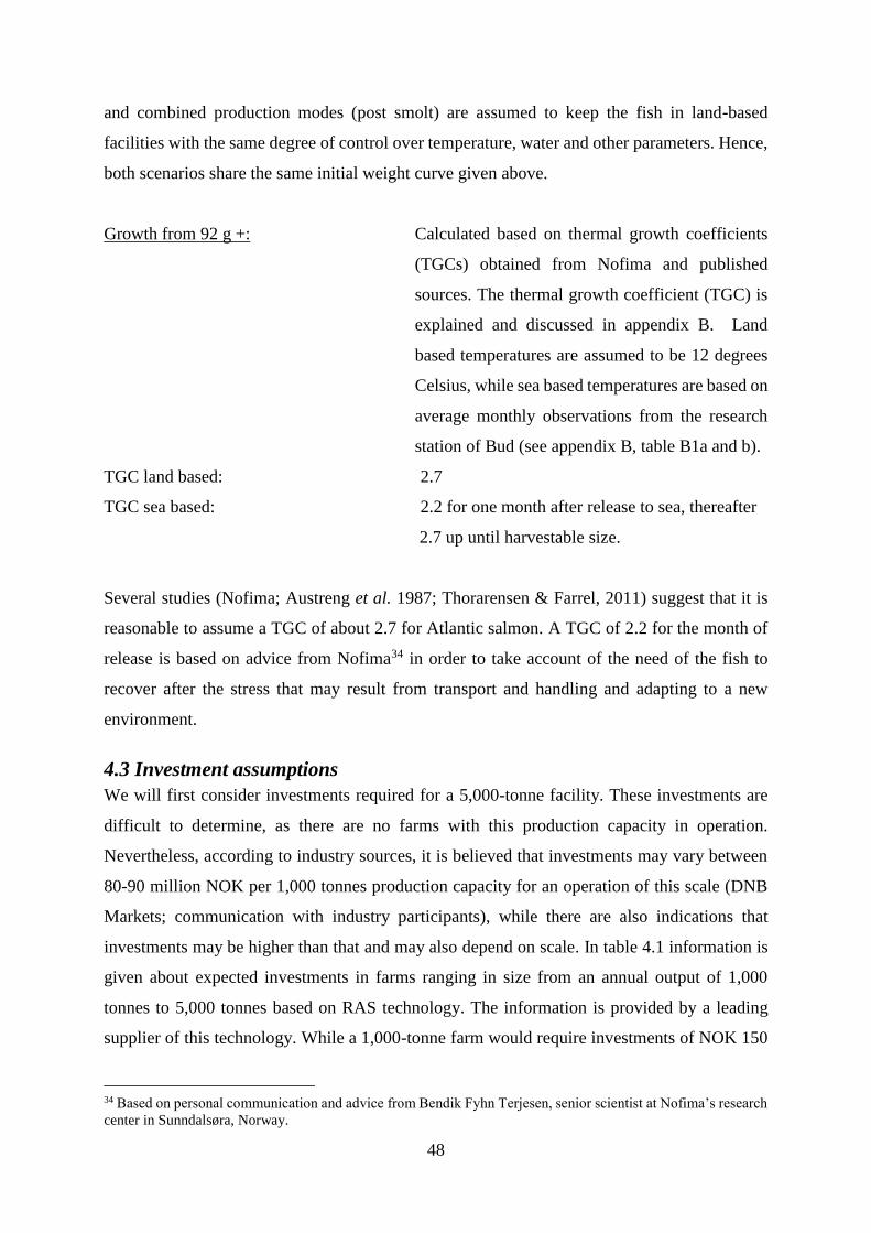
48

and combined production modes (post smolt) are assumed to keep the fish in land-based

facilities with the same degree of control over temperature, water and other parameters. Hence,

both scenarios share the same initial weight curve given above.

Growth from 92 g +: Calculated based on thermal growth coefficients

(TGCs) obtained from Nofima and published

sources. The thermal growth coefficient (TGC) is

explained and discussed in appendix B. Land

based temperatures are assumed to be 12 degrees

Celsius, while sea based temperatures are based on

average monthly observations from the research

station of Bud (see appendix B, table B1a and b).

TGC land based: 2.7

TGC sea based: 2.2 for one month after release to sea, thereafter

2.7 up until harvestable size.

Several studies (Nofima; Austreng et al. 1987; Thorarensen & Farrel, 2011) suggest that it is

reasonable to assume a TGC of about 2.7 for Atlantic salmon. A TGC of 2.2 for the month of

release is based on advice from Nofima34 in order to take account of the need of the fish to

recover after the stress that may result from transport and handling and adapting to a new

environment.

4.3 Investment assumptions

We will first consider investments required for a 5,000-tonne facility. These investments are

difficult to determine, as there are no farms with this production capacity in operation.

Nevertheless, according to industry sources, it is believed that investments may vary between

80-90 million NOK per 1,000 tonnes production capacity for an operation of this scale (DNB

Markets; communication with industry participants), while there are also indications that

investments may be higher than that and may also depend on scale. In table 4.1 information is

given about expected investments in farms ranging in size from an annual output of 1,000

tonnes to 5,000 tonnes based on RAS technology. The information is provided by a leading

supplier of this technology. While a 1,000-tonne farm would require investments of NOK 150

34 Based on personal communication and advice from Bendik Fyhn Terjesen, senior scientist at Nofima’s research

center in Sunndalsøra, Norway.

49

million, this increases to NOK 578 million for a 5,000-tonne farm. In all alternatives, RAS

equipment is the largest share of the investments, followed by buildings and concrete work

(RAS and fish tanks).

Table 4.1: Investments in land based farms from 1,000-5,000 tonnes. NOK ‘000.

Investment (NOK)a) 1000t 2000t 3000t 4000t 5000t

Buildings 41,424 66,218 86,616 113,433 159,062

Electrical

installations 9,212 17,001 20,169 26,414 31,553

Other installations

(ventilation etc.) 7,646 13,935 14,953 19,583 22,131

RAS equipment 67,179 110,249 156,395 204,815 245,902

Concrete work (RAS

and fish tanks) 19,302 62,854 70,378 92,167 108,608

Various 5,013 5,574 6,955 9,108 10,820

Total investment 149,776 275,830 355,467 465,520 578,076

Investment

NOK/kg

production 149.8 137.9 118.5 116.4 115.6

a) Note: Values are originally in Euros (€) and have been converted to NOK using the

2016 average NOK/USD exchange rate: 9,2899 (the Central Bank of Norway).

Source: Billund Aquaculture Service A/S.

Investment per kg of production capacity gives an indication of economies of scale in

production. Investment is NOK 149.80 per kg production capacity for the 1,000-tonne farm

and starts levelling off for the 3,000-tonne farm (NOK 118,50/kg) to NOK 115.60 for the 5,000-

tonne farm. With the exception of concrete work, all other parts of the investments appear to

give rise to economies of scale.35

As our base case, we will use information that has been made available from one planned

5,000-tonne project. Investments, which are given in table 4.2, have been quality controlled by

industry participants with some indications that they may be located at the lower end of the

likely investment range (see also table 4.1 for comparison). As noted above, the technology

selected is that of RAS. Total investments are estimated at NOK 429.3 million. This

corresponds to investment of NOK 83.85 per kg production capacity. While this is in the range

considered “normal” by many industry participants, it is considerably lower than the figures in

table 4.1. As there are very few such farms in operation, this discrepancy cannot be resolved

by empirical observations. We will, however, perform a sensitivity analysis so as to quantify

35 For a full picture of economies of scale, it is also necessary to consider other costs of production that do not

increase proportionally with output such as labour and management. This will be discussed in chaper 4.5.

50

the consequences of different assumptions regarding investment costs when it comes to cost of

production and net present value.

The main investment components are building, construction and project related work

(NOK 206.6 million), aquaculture system equipment (RAS and related equipment such as

piping, pumping and electric equipment, NOK 181 million), investment in land, infrastructure

connection and ground water drilling (NOK 12 million). Fish management and laboratory

equipment amounts to approximately NOK 6.0 million, production tanks and hardware to NOK

5.0 million while cost of planning is set to NOK 1 million.

Table 4.1. Investments and Annual Depreciation and Interest for a 5,000-tonne salmon farm.

NOK ’000

Investment,

NOK (‘000)

Economic

lifetime

Depreciation

and interest,

NOK (‘000)

Building, construction and project related costs 206,641 20 15,205

Aquaculture system equipment (pumping, piping,

filter, water treatment & electric)

180,905 20

13,311

Production tanks and hardware 5,000 20 368

Fish management, feeding and heating systems,

vaccination and laboratory equipment

6,011 10

741

Land/building plot (60,000 m2) and plot development 12,000 - 480

Infrastructure connection (road, electricity, plumbing)

and ground water drilling

18,000 -

720

Cost of planning, application, processing fee, etc. 1,042 - 42

Sum 429,600 30,867

Investments provide the basis for estimating the company’s capital cost, represented by

interest and depreciation on invested capital. As noted above, the interest rate is set at 4%. For

estimation of annual depreciation charges on the physical structures that depreciate over time,

the lifespan (amortisation period) is assumed to vary from 10 to 20 years for different

components (table 4.1). Often, depreciation is based on a linear method or a certain percentage

of the remaining value per year, which means that the annual depreciation will vary over time

(Asche & Bjørndal, op.cit, 209). In this case, an annualised depreciation and capital cost is

estimated according to the annuity principle, making the sum of interest and depreciation a

steady annualised cost (ibid.)36. Land does not depreciate and therefore only interest is charged.

The same is done for the cost of planning, application and processing fee related to establishing

the project and obtaining an operating permission (license). As shown in table 4.1, the sum of

36 Annuity factors are 0,0736 for 20 years, 0,0899 for 15 years and 0,1233 for 10 years.

51

interest and depreciation amounts to NOK 31.7 million annually, which can be considered the

average amount of depreciation and interest over time (ibid.).

With investments as outlined above, an operational farm is established with capacity to

produce annual harvests of 5,000 tonnes. In the following, a production plan tailored to the

facility’s capacity will be outlined, providing the basis for calculating steady state cost of

production.

4.4 Production plan

In salmon aquaculture, the biological process associated with growing salmon to harvestable

size is the foundation of the operation. The company’s production plan consists of biological

variables such as hatching, smolt release, feeding, mortality and biomass growth. In turn, this

constitutes central inputs to the estimation of cost of production.

Continuing with the case study, the production plan for an annual harvests of 5,000

tonnes is presented. To maintain a high capacity utilisation at all times, salmon is harvested and

released to the facility on a monthly basis. Roe is delivered to the operation every month at a

quantity of 113,500 eggs. Within 6-10 weeks, eggs are transformed into fry37 which are released

into tanks where they start being fed for about nine additional weeks. The monthly release of

0.2-gram fry to the “start feeding tanks” is 102,150 fish. The weight curve for individual salmon

is illustrated in figure 4.1, where the salmon grow from an individual size of 0.2 g in month 0

to 5 kg by the end of month 18. Harvest is 416.8 tonnes per month starting in month 18.

Figure 4.1: Weight curve for salmon – weight in grams per fish. Month 0-19.

Table 4.2 presents the main parameters of the production plan (with further details given

in Appendix, table C1). Monthly releases of 102,150 fry give monthly harvests of about 90,000

37In this period, the roe hatches and the larvae initially receive their nutrition from a yolk sac which forms part of

their body. As time passes, the larvae grow while the yolk sac diminishes. When the yolk sack has eroded about

¾, the term fry is used for to describe the tiny fish which must become capable of feeding themselves.

0

1 000

2 000

3 000

4 000

5 000

6 000

0 1 2 3 4 5 6 7 8 9 10 11 12 13 14 15 16 17 18 19

Wei

ght

per

fis

h (

g)

Month

52

grown-up salmon in full, steady state production, each fish at an average individual weight of

4.6 kg after 19 months of growth. The individual harvest weight will vary somewhat, as harvest

is done over time throughout the month of harvest, over 19 working days. This gives a monthly

harvest of about 416.8 tonnes, corresponding to daily harvests of about 22 tonnes.

Before harvest, the fish are often starved for some time38. This means that for a certain

period, both feeding and growth is reduced. In the analysis, we simplify by assuming monthly

harvest equal to the average weight per fish between the start of the harvest month and the end

of the harvest month (if it is fed) times the average number of fish in the month given the

assumed mortality. In the month of harvest, feeding is calculated on the basis of half of the

average number of fish being fed (if no harvest was undertaken).

Table 4.2. Production plan

Fish harvest size 4.6 kg (range 4.2-5 kg throughout month 18)

Production period

Hatchery: 6-10 weeks to 0,2 g (start feed)

On-growing: Release of 0.2 g fry in month 0, with harvest in month

18

Monthly purchase of

roe 113,500 eggs

Mortality

Hatchery (from egg delivery to 0,2 g): 10%

Mortality in the initial start feeding month: 4%, then subsequently

0.5% per month. Over the life cycle, this gives a total mortality of 21%

(including the roe stage), whereof 14% occurs up until a fish size of 3

g

Number of 0.2 g fry

released 102,150 fry per month

Price of roe NOK 1.00 per egg (range 1-1.6 depending on breed)

Vaccination NOK 1.8 per vaccine (range 1.5-2 per vaccine depending on contents)

On average 95,877 fish per batch (monthly vaccination at 71 g)

Annual production 5,000 tonnes

Harvest Monthly harvest is 416.8 tonnes, starting from month 18 (year 2).

Biological feed

conversion ratio

(FCR)

0.9 in months 0-11 (800 g), then subsequently 1.1

Annual feed quantity:

5,383 tonnes (appendix C), given the assumptions above

38 In land based aquaculture, it is also often necessary to allow for a pre-harvest practice called purging, where the

fish are held in flow-through tanks for about two weeks before harvest. The reason for this is that some particles

that accumulate in RAS systems cause the salmon flesh to get an “off-flavour”, sometimes described as a muddy

taste. These particles are removed from the fish when it is allowed to swim for at least two weeks in flow-through

tanks, with constant water exchange rather than recirculation. The process happens faster if the fish gets exercise

in the tanks, preferably with currents at the speed of one fish-length per second, which is indicated to shorten the

required purging time by up to 40% (Nofima).

53

Feed price NOK 14 per kg

Sources:

Salmobreed for egg price.

EWA Consulting and industry sources for price of vaccines and feed.

Industry sources (0.2 g – 92 g) and Nofima (92 g +) for growth data and biological FCR.

A combination of company sources and own judgement for mortality assumptions.

On the basis of this production plan (see appendix, table C1), the annual feed quantity

is estimated to 5,383 tonnes which gives an economic FCR of 1.08. Given a feed price of NOK

14 per kg (table 4.2), this gives an annual feed cost of NOK 75,36 million when fully

operational.

Assumptions about other costs are given in table 4.3. The required number of full-time

workers is estimated 16 in the hatchery and production departments. Given labour costs of NOK

665,000 per person-year, annual labour costs amount to NOK 10.64 million. As the table shows,

several cost categories including feed, oxygen and wastewater treatment are directly related to

the quantity produced. The consumption of water depends on the technology and the production

quantity in order to maintain the desired water quality. In this example, investment in a water

well is assumed (fresh ground water), so that there are no direct costs associated with water

intake and consumption apart from electricity costs39. Alternatively, water may be purchased

from the municipal water system at a price of about NOK 7 per m3. Variable costs such as office

and administration, service, maintenance and repairs are somewhat more loosely tied to

production quantity.

In addition, fixed costs of management (four managers) amount to NOK 3.9 million.

Because of the long production period for salmon where capital is tied down in the biomass

production process, the operations also require large investments in working capital.

Table 4.3. Cost Assumptions.

Cost assumptions:

Variable costs

Number of man-years 16 in production

Electricity NOK 1 per kwh. (including “network rental fee” and

“electricity fee”)

4 kwh per kg of production (range 3-4 kwh per kg)

20 million kWh per annum

Oxygen NOK 2.50 per kg (range 2-2.5)

2,817 tonnes per annum (0.5 kg per kg of feed)

39 Investments required to establish a ground water source could vary widely depending on the sources of ground

water available as well as on the type of soil or bedrock. Costs associated with maintaining the desired level of

salinity in the water are assumed to be incorporated in the cost category labelled “other costs”.

54

Oxygen storage tank rental: NOK 150,000 per annum (range

100-200,000)

Waste/wastewater NOK 800 per tonne (range 130-2000).

8,380 tonnes per annum (1.5 kg per kg of feed, not dried)

Service, maintenance and

repairs

NOK 3.5 million per year (range 3-4 million)

Office and administration NOK 1.5 million

Other costs NOK 10 million

Includes laboratory, salinity, other chemicals, etc.

Fixed costs

Management Four managers

Sources:

Industry sources including equipment suppliers, smolt producers and potential/new entrants

(full grow-out) for price and consumption of electricity and oxygen.

Equipment suppliers and industry sources for quantity and cost of sludge/waste disposal.

A combination of company sources and own judgement for service, maintenance and repairs

and office and administration cost.

4.5 Cost of production

As described in chapter III, to analyse cost of production a steady state situation is assumed,

meaning that the farm is fully operational (Asche & Bjørndal, op.cit). Among the benefits

associated with land based aquaculture is the possibility of releasing batches of juveniles

throughout the year so as to have harvestable fish all year around. As illustrated in the

production plan, this example has a monthly release of 102,150 fry into the facility. The total

amount of salmon harvested in one calendar year will be the same as the harvest from the 12

releases in a year (see appendix, table C1). Hence, annual costs and cost of production are

estimated on the basis of 12 releases.

Table 4.4 specifies other operating costs per annum. These costs amount to NOK

9.70/kg, which is higher than the NOK 6.31/kg in traditional farming (chapter II, table 2.1).

This may be explained by the difference in technology. Other operating costs include electricity,

oxygen, bicarbonate (alkalinity), sludge/waste cost, service, maintenance and repairs, office

and administration, and other annual operating costs (laboratory, salinity, other chemicals etc.).

Table 4.4 Other operating costs

Unit Quantity Price/

Unit

Steady

state

NOK ‘000

Per

kg

Electricity

4,000 kwh per tonne of

production

20,484

kwh 1 20,484 4,1

Oxygen

0.5 tonnes per tonne of

production 2,560 t 2,5 6,401 1,3

Oxygen - tank rental annual cost (NOK ‘000) 150 0,0

Sludge/waste/wastewater 1.5 tonnes per tonne of feed 8074,7 t 800 6,460 1,3

Service, maintenance

and repairs annual cost (NOK ‘000) 3,500 0,7

55

Office and adm. annual cost (NOK ‘000) 1,500 0,3

Other annual operating

costs annual cost (NOK ‘000) 10,000 2,0

Sum 48,494 9,7

In table 4.5, total annual cost of production in steady state is given as well as average

cost per kg produced. Total production cost amounts to just over NOK 181 million. While

variable costs represent 80 percent, fixed costs are 20 percent of the total. The most important

components are feed, interest and depreciation on investments and other operating costs.

Average cost of production per kg of salmon in “live weight” is NOK 36.3. To be comparable

with official statistics, this must be converted to whole fish equivalents (WFE), using standard

ratios (The Norwegian Directorate of Fisheries, 2016; See also table 4.5 below, comment c)).

In WFE terms, the cost of production per kg of salmon is NOK 38.7.

Because of substantial working capital requirements, interest on working capital at 4%

can constitute a considerable cost component and is therefore included as a variable cost.

Table 4.5: Cost of production

Total cost

NOK ‘000

NOK/kg

live weight

Percent of

total

(WFE)

NOK/kg

WFE

Variable:

Feed 75 364 15,1 42 % 16,1

Roe (smolt) 1 362 0,3 1 % 0,3

Vaccines 2 071 0,4 1 % 0,4

Labour 10 640 2,1 6 % 2,3

Insurance fish 3,448 0.7 2 % 0,7

Other operating costs 48,494 9,7 27 % 10,3

Interest on working capitala) 4,620 0,9 3 % 1,0

Sum variable costs 145 999 29.2 80 % 31,2

Fixed:

Interest and depreciation

on investments 30 867 6,2 17 % 6,6

Insurance on building and equipmentb) 604 0,1 0,3 % 0,1

Management 3 900 0,8 2 % 0,8

Sum fixed costs 35 371 7,1 20 % 7,5

Total production cost 181,370 36,3 100 % 38,7

a) Interest on working capital is on the basis of feed, roe, vaccines, labour, other operating

costs, insurance and management costs.

b) Building is considered building, construction and project related costs, total NOK 206.6

million. Equipment and machinery is aquaculture system equipment, tanks and

hardware, fish management, feeding and heating systems, vaccination and laboratory

equipment, total NOK 192 million (table 4.1).

c) In accordance with NS 9417:2012 and the current practice of the Norwegian Directorate

of Fisheries, the conversion factor from live weight to WFE is 1.067.

56

When compared to sea based farming (table 2.1, chapter II), it is noticeable that cost of

production per kg is higher in the case of full cycle land based farming. It must, however, be

noted that the numbers in this chapter are 2017 values as compared to 2015 values in table 2.1.

Furthermore, interest on license values is not included in table 2.1 (as discussed in chapter II).

Comparing different cost categories, it can be noted that feed cost is slightly higher

(NOK 14.40/kg as compared to NOK 13.18/kg) This is understandable, as the price of feed is

assumed to be somewhat higher in land based aquaculture. In recirculating aquaculture systems,

where nearly all of the water is filtered and reused repeatedly, feed quality including texture is

particularly important for water quality. In terms of feed cost, it can also be noted that the fish

in land based operations are grown and fed from the time of hatching, versus from a size of

approximately 100 grams in the case of traditional sea-based grow-out operations. However,

this difference in absolute feeding and growth of 100 g is not likely to make up a large part of

the difference in feed cost per kg40.

Land based aquaculture is also a technologically more advanced operation, which is

reflected in the cost shares. Notably, interest and depreciation on facility and equipment

constitute 17% of the total, amounting to NOK 31 million per annum (NOK 6.6/kg). This

compares to NOK 3.97/kg or 14% of the total in sea based production (including own estimate

for license values from the discussion in chapter II), with the difference being that in sea based

production, license investments are the cost driver, while in land based production, investments

in technology and facility drives the capital costs.

4.6 Net Present Value

For potential investors in a land based salmon farm, what is of interest is whether they will

achieve an acceptable return on the capital invested. Evaluating the value of a company requires

information about the cash flows it will generate. The objective for the investor is then to

determine if the initial investment will provide a positive net present value (NPV) of cash flows

given the investor’s required rate of return (interest rate) as outlined in chapter III, see equation

4.1.

40 Assuming an economic FCR of 1, the feed quantity required to grow the smolts up to a size of 100 g is 100 g.

Given a feed price of NOK 15 (smolt feed) and a harvest weight of 4.5-5 kg, the difference in feed cost due to the

feeding of smolts should be roughly NOK 0.3-0.33/kg. Hence, the majority of the NOK 1.22 difference in feed

cost seems to stem from difference in feed price or mortality assumptions rather than the difference in feeding

period.

57

We can identify three types of cash flows in this case, namely those related to (i)

investments and reinvestments, (ii) revenues from the sale of fish and (iii) operating costs such

as feed and labour.41 It is assumed that revenues are received in the same period as the fish is

sold, while feed, labour and other inputs are paid in the period they are incurred. To carry out

the analysis, information in previous sections will be used to determine the cash flows. The net

present value analysis assumes that the production facility is delivered as a fully developed,

turn-key facility in year 0 with investments of NOK 420 million. Moreover, all necessary

permits, licenses and planning have been acquired. Hence, the first monthly purchase of roe

may be scheduled for January 1st of year zero. After about two months in the hatchery, the first

batch of 102,150 fry are released to feeding tanks on March 1st the same year. Following 18 full

months of grow-out, the first batch of salmon is harvested in September of year one. It follows

that from year two steady state production is reached, where salmon are released and harvested

monthly, with an annual harvest of 5,000 tonnes.

In the estimation of net present value, we will assume that prices and costs remain at the

same level, i.e., real prices remain unchanged. Assumptions about annual costs and revenues

are summarised in table 4.6. The following operating costs are included: roe, feed, labour,

vaccines, operating costs, management and facility investment. Financial costs – interest on

fixed investments and working capital as well as depreciation – are not included, as the cost of

capital is accounted for by including investments (and reinvestments) and the interest rate,

representing the required return on capital. Moreover, depreciation does not involve any cash

outlay.42

Table 4.6. Assumptions about costs and revenues years 0-2. Monetary values in NOK ‘000.

Assumptions: Year 0 Year 1 Year 2 (steady

state, as above)

Variable costs

Roe NOK 1,362 NOK 1,362 NOK 1,362

Feed quantity 138.8 tonnes 3,495.6 tonnes 5,383,1 tonnes

Feed costs NOK 1,943.5 NOK 48,937.8 NOK 75,363,9

Number of man-years 6 12

16

Labour costs NOK 3,990.0 NOK 7,980.0 NOK 10,640.0

Insurance fish NOK 579.0 NOK 2,258.8 NOK 3,448.3

No of vaccines 5 batches 12 batches 12 batches

Vaccine cost NOK 517.7 NOK 2,070.9 NOK 2,070.9

41 In principle, there can also be a terminal value of the investment. 42 The situation would be different if taxes were included. This because depreciation influences taxable income

and thus taxes paid.

58

Other operating costs NOK 15,000.0 NOK 30,000.0 NOK 48,494.4

Fixed costs

No of managers 2 4 4

Management costs 1,950.0 NOK 3,900.0 NOK 3,900.0

Insurance on facility and

equipment

NOK 603.8 NOK 603.8 NOK 603.8

TOTAL COSTS NOK 25,712.1 NOK 94,854.5 NOK 145,883.3

Price & revenue

Salmon price NOK 59/kg (HOG)a), i.e., 49.2 (live weight)b)

Harvest quantity 0 4 batches, each of

416.8 tonnes

12 batches, 5,000

tonnes

Revenue 0 NOK 98,365 NOK 295,000 a) The average forward contract price from March 2017 to December 2019, obtained from

fishpool.eu per March 2017. The price is based on an index of fish sizes, premium

quality and HOG weight b) As the production quantity is given in live weight, the price is converted to live weight

in order to estimate corresponding revenues. A conversion rate from live to HOG of 1.2

is used, in line with NS and the Directorate of Fisheries. (This does not consider that

processing costs are incurred between live and HOG weight. Consequently, the HOG

price assumed here may not reflect the cost of processing).

Whereas full steady state cost of production is incurred from year two, the first two years

of production see lower, yet increasing costs of production as biomass is built up and increasing

amounts of capital are tied up in the fish stock. In terms of production workers, six are employed

for 1st January year zero, another six are employed at the beginning of year one, while the full

complement of 16 will be active from 1st January year to. Two managers are hired from the

opening of the plant; the two additional ones on January 1st, year 1. Other operating costs

increase over time to reach steady state. Feed costs are also considerably lower than in steady

state while the biomass is being developed from scratch.

Total costs increase from NOK 25.71 million in year 0, to NOK 94.83 million in year 1

and to a steady state level of NOK 145.88 million in year 2. The increase is mainly due to feed,

labour and other operating costs.

As for revenues, the first harvest of 416.8 tonnes occurs in December year one. As of

year two, steady state harvesting takes place. When it comes to price, we need to use the

expected price for the lifetime of the project. In view of historical fluctuations in price, this is,

of course, impossible to assess. Initially, we will use NOK 49.20/kg, which is slightly less than

the average forward price from March 2017 – December 2019 per February 2017, but notably

still high from a historical perspective (Fishpool, 2017). For comparison, the average price

between 2011-2017 (week 7) is NOK 41.30/kg. There are no revenues in year 0, NOK 98.368

59

million in year 1, and from year 2 onwards the steady state annual revenues represent NOK 295

million.

As such, annual cash flows over time from investments and reinvestments, revenues and

costs are established. These are given in table 4.7.

As shown in table 4.1, while most equipment will have a lifespan of 20 years, some

have a depreciation period of 10. For simplicity, we assume the production technology remains

unchanged over time so that only a reinvestment of NOK 6 million is included.

Table 4.7. Annual cash flows: investments, revenues and costs. NOK million.

Year Investment and

reinvestment

Revenues Costs

0 429.6 0 25.712

1 81.963 94.855

2 245.889 145.883

3 245.889 145.883

4 245.889 145.883

5 245.889 145.883

6 245.889 145.883

7 245.889 145.883

8 245.889 145.883

9 6.0 245.889 145.883

10 245.889 145.883

11 245.889 145.883

12 245.889 145.883

13 245.889 145.883

14 245.889 145.883

15 245.889 145.883

16 245.889 145.883

17 245.889 145.883

18 245.889 145.883

19 245.889 145.883

20: terminal

value

669.621a) 6,147.225 3,647.075

a) This includes investments and reinvestments from year 20 to year 60. See appendix,

table C3 for the investment and reinvestments used.

When valuing a company, there is a question as to the time period over which the

investment should be considered. There is no definite answer to that question. We will choose

two alternatives. The first is an investment horizon of 20 years43. This seems natural, as this

43 It might seem natural to include a terminal value for this case. The terminal value may be positive if land and

machinery may be sold. It may also be negative, in case the owners need to pay more for the disposal of the facility

than proceeds from sale of the land. As it is impossible to determine the value, we will disregard the terminal

value.

60

is the lifespan of most of the technical equipment44. It is, however, also natural to consider an

infinite time horizon. This is because if the initial investment turns out to be profitable, a

reinvestment is likely after 20 years. For the infinite horizon case, we will assume this to be

the case. This assumes that the production technology remains unchanged. This is, of course,

a very strong assumption, but as reasonable as any other to be made.

For the case of an infinite time horizon, we have estimated the terminal value in year

20. For investments, this is the present value in year 20 of investments up to year 60 (appendix,

table C3). Due to discounting, the setting of a cutoff year like often has a small impact on the

terminal value. Revenues and costs are both constant in steady state so that the terminal value

in year 20 is calculated according to the formula A/r, where A is the annual amount and r the

rate of interest.

All values are discounted to year 0 according to the formula in chapter III (equation

4.1). Year 0 values are not discounted, year 1 values are discounted one year, etc. In doing so,

it is assumed that all revenues and expenses are incurred on a linear basis throughout the year.

This is not quite correct, as there is likely to be an uneven time profile for some of the outlays.

Nevertheless, this simplification will have little impact on the result.

The results are given in table 4.8. With a 20-year horizon, the NPV is NOK 745.4

million while for the case of an infinite time horizon, it is NOK 1,580.8 million, more than a

doubling. This is due to the rather large net terminal value. The IRRs are 17% and 19%,

respectively.

All of these values indicate a very profitable investment. It must be noted that this

assumes the farm runs smoothly from day one without any problems. In light of the

development of the industry over time (chapter II) and in consideration of the fact that we are

considering a new technology, this could be unreasonable. Nevertheless, while the industry has

been growing rapidly for several decades, it has been very profitable for long periods of time,

in particular recently.

Table 4.8. Net present value (NOK million) and internal rate of return.

20 year horizon Infinite horizon

NPV NOK million 745.4 1,580.8

IRR 17% 19%

44 King et al. (2016), in their study of alternative production models for Tasmania, estimate NPV for a 15-year

timespan.

61

A number of simplifying assumptions have been made in the estimation of NPV and

IRR, in particular that the price and cost of production remain constant over time. In view of

the fact that both price and cost have been changing over time (chapter II), there is every reason

to expect this to be the case also in the future. For this reason, we will undertake sensitivity

analyses for changes in price and costs below. Moreover, we have assumed the technology

remains unchanged over time. This is unrealistic, in particular, because we are considering a

new technology that is largely untried in salmon farming. Thus, it is likely there will be many

adjustments in technological solutions in the coming years.

It would be possible to include time trends for future developments in price and costs in

addition to the discrete changes that will be considered in the sensitivity analyses below. This

will not be done, as it appears very difficult to specify realistic time trends. Having said that,

as producers master the new technology to a greater degree, this will represent improvements

in technology and thus reductions in cost of production. This will make the investment even

more profitable, which is likely to cause an increase in production that will have a dampening

effect on price. The net effect of this is likely to be a reduction in profitability so that the NPV

that has been presented here is likely to be overestimated.

It is noticeable that the NPV for an infinite horizon-project is almost twice that for a 20-

year time horizon. As noted, there is great uncertainty about future prices and costs and more

so, the longer the time horizon. For this reason, we will subsequently present results for a 20-

year horizon only. This raises the question of a scrap value after 20 years. As discussed above,

this can be positive or negative. The scrap value will here be set to zero, as it does not seem

possible to set a meaningful value.45

4.7 Sensitivity analyses

As discussed not only here, but also in previous chapters, due to the dearth of empirical data

there is great uncertainty as to the appropriate values of many important parameters included

in this analysis. One way to address this issue is by use of sensitivity analysis (chapter III).

With this approach, it is possible to identify the impact of uncertainty in a parameter on cost of

production and NPV. Moreover, it is possible to vary several parameters at the same time so as

to analyse their combined effect.

45 DnB Markets (2017) use a decommissioning cost/scrap value after 20 years of NOK – 30 million (based on a

10,000-tonne project), but there is no explanation as to how this value was arrived at.

62

4.7.1 Cost of production

We will now analyse how cost of production may vary with changes in important parameters

and assumptions. The following parameters have been selected for sensitivity analyses:

1. Investments + 20 %.

2. Other operating costs + 20 %.

3. Monthly mortality + 20 %.

4. Late-cycle mortality: 20%

5. Growth – 20 %.

6. FCR +20%

7. Interest rate 8 %.

Essentially, all these changes are due to the introduction of a fairly new technology with only

limited experience. 1) and 2) refer to uncertainty about investment as well as operating costs.

3), 4) and 5) refer to uncertainty about the biological production function. In principle, we could

envisage two scenarios in the case of mortality and growth. In the first case, higher mortality or

lower growth is anticipated so that this is corrected for by the purchase of more roe so that a

5,000-tonne production can be maintained. In the second scenario, which will be considered

here, there is no such compensation causing a reduction in output of about 20% (in the two

examples involving late-cycle mortality and reduced monthly growth). Results are presented in

table 4.9. While both positive and negative changes are presented in table 4.9 and illustrated in

figure 4.2, the following discussion is focused on the downside risk.

Table 4.9. Sensitivity analysis for cost of production– NOK/kg (WFE).

-20 % Base case 20 %

Investment 37,4 (-3%) 38,7 40,0 (+3%)

Other operating costs 36,5 (-3%) 38,7 40,9 (+6%)

FCR 35,0 (-10%) 38,7 42,4 (+10%)

Monthly mortality 37,9 (-2%) 38,7 39,5 (+2%)

Late-cycle mortality - 38,7 46,7 (+21%)

Growth 42,2 (+9%) 38,7 36,3 (-6%)

Interest rate 8%: Cost/kg = 42,3 (+9%)

With a 20% increase in investments, these now become NOK 515.5 million, resulting in higher

interest and depreciation charges. Moreover, there will be a slight increase in insurance on

building and equipment. The consequence of this is a 3.4% increase in cost of production to

NOK 40.0/kg. A proportional increase of the same magnitude in other operating costs will cause

an increase in cost of production of 5.7% to NOK 40.9/kg, a small part of which is attributable

63

to an increase in working capital and thereby the consequences of a small increase in interest

on working capital.

Regarding mortality, two scenarios are considered. In the first one, there is a 20%

increase in monthly mortality throughout the lifespan of the fish46. This results in a decrease in

the annual harvest quantity to 4,764.7 tonnes, with a 2% increase in cost of production to NOK

39.50/kg. It may be surprising the cost of production changes so little. The cost structure is

characterised by large variable costs, and higher mortality implies a reduction in many of them

(feed, vaccines, insurance and interest on working capital). Moreover, the increase by 20% is

added to a low mortality rate in the first place – increasing from 0.5% to 0.6% of individuals

per month of on-growing. During the period of higher mortality – the egg stage and initial start

feeding month – relatively little cost has been accumulated per fish.

We also consider the consequence of late-cycle mortality. This kind of issue can occur

as a consequence of early maturation or quality degradation of soon-to-be harvested fish. Such

challenges have been of major concern throughout the production phase in existing land based

operations and constitute an important part of the biological risk in this new type of biological

environment. In this example, it is assumed that in month 16, 20% of the number of fish per

generation die. This gives a new accumulated mortality of 29.3% from start feed to harvest, or

36.4% when the egg stage is included. Under this assumption, the annual harvest quantity

becomes 4,021 tonnes. The consequence will be an increase in cost of production of 21%

compared to the base case to NOK 46.7/kg.

The modified growth case involves a 20% lower fish weight compared to the base case

in each month, starting from month one. Hence, in month 18, the batches are harvested at an

average weight 20% less than the base case (3.7 kg vs 4.6 kg). In this case, the annual harvest

becomes 4,000 tonnes, causing a 9% increase in cost of production to NOK 42.20/kg.

A modified feed conversion ratio is included because of the considerable share of feed

in total costs – although the share is a bit lower than in sea based production. An increase in

FCR by 20% is estimated to cause cost of production to increase to NOK 42.4/kg, an increase

by 9.6%.

46 New mortality: hatchery: 10%*1.20 = 12%; month 0 (start feed): 4%*1.2 = 4,8%; all subsequent months of on-

growing: 0.5%*1.2 = 0.6%. In total, the new accumulated mortality is 24.6%, compared to 20.9% before.

64

Figure 4.2: Sensitivity analysis for cost of production– NOK/kg (WFE).

A doubling of the interest rate has been specified due to the risk involved, despite the

fact that we are looking at investments from society’s point of view (cf. chapter III). In this

scenario, we assume that the depreciation periods remain unchanged. With an interest rate of

8%, annual interest and depreciation charges increase from NOK 30.9 million (table 4.1) to

NOK 43.4 million. As a consequence, cost of production per kg increases by 9.3% to NOK 42.3

(interest on working capital is also part of the change).

As underlined, we are talking about a new technology so that empirical data on cost of

production are non-existent. Nevertheless, a number of engineering studies have been made.

Table 4.10 summarises results from some of these studies. The specification of the cost structure

is different from study to study, for example when it comes to inclusion of costs such as

insurance and interest on working capital. We have therefore restated the cost components in

terms of the categories that are found in all comparable studies.

Table 4.10. Estimates of cost of production in land based salmon farming. NOK/kg.

Land based

Norway,

Iversen et al.

(2013)a)

Land based

low cost

country,

Iversen et al.

(2013) a)

Liu et al.

(2016)

WFEb)

DNB

(2017)

WFE

This study

WFE

Feed 9,8 9,8 11,8 13 16

Smolt (roe) 1,9 1,0 0,8 2 0.3

Salaries 2,4 1,2 3,3 3 3.1c)

Other operating costs 6,0 4,4 10,7 6 11.4d)

Depreciation and

interest 8,5 6,2 7,6 6

6.6

Production cost total 28,6 22,6 34,2 30,0 38.7

65

a) It is not found whether this cost is based on live weight or WFE. However, the base case

used for comparison in the study is the Norwegian Directorate of Fisheries’ statistics,

which are given in WFE weight.

b) Liu et al. report cost per kg HOG. This cost has been converted to WFE-cost using a

factor of 0,089 in accordance with the Norwegian Directorate of Fisheries and the

Norwegian standard.

c) Includes wages (NOK 2.3/kg) and management (NOK 0.8/kg)

d) Includes interest on working capital (NOK 1.0/kg) and insurance (NOK 0.1/kg)

Cost of production per kg is highest in this study and lowest in Iversen et al. (2013).

However, the latter is in 2013 values rather than 2017. Feed costs are considerably higher in

this study than in all the others while smolt cost (roe in this study) are lower. Even if feed prices

have been rising in recent years, the feed price in the current study is set quite high, based on

information about the extra importance of feed and feed particles to water quality in recycling

water systems47. Wage costs are comparable for four of the studies, while other operating costs

are considerably higher in this study and Liu et al. (2016) than all the others. Depreciation and

interest are also comparable in some of the studies.

4.7.2 NPV and IRR

To analyse senstitivity of NPV and IRR, we will consider the following scenarios:

1. Investments +/- 20 %

2. Other operating costs +/- 20 %

3. Total operating costs +/- 20%

4. FCR +/- 20%

5. Monthly mortality +/- 20 %

6. Late-cycle mortality +20%

7. Growth +/– 20 %

8. Price +/– 20%.

The first five are the same as for cost of production, however, we have also included a scenario

analysing variation in price of 20%. This because there is much uncertainty about which price

level can be expected in the future. Results are given in table 4.11.

Table 4.11. Sensitivity analyses NPV and IRR. 20-year lifespan.

NPV IRR

-20 % Base case 20 % -20 % Base case 20 %

Investment 834 (+12%) 745

657 (-12%) 21 % 17 %

14 %

Other operating costs 866 (+16%) 624 (-16%) 19 % 15 %

47 The difference in feed costs may also be due to differences in variables such as mortality and FCR.

66

Monthly mortality 833 (+12%) 661 (-11%) 18 % 16 %

FCR 959 (+29%) 531 (-29%) 20 % 14 %

Total cost of prod. 1,124 (+51%) 367 (-51%) 23 % 11 %

Late-cycle mortality - 210 (-72%) - 8 %

Growth 412 (-45%) 1,079 (+45%) 12 % 22 %

Price 131 (-82%) 1,360 (+83%) 7 % 26 %

Interest rate 8% NPV = 398 (47%) IRR = 17 %

A 20% reduction in growth and a concomitant reduction in output is seen to reduce NPV

by about 45% compared to the base case, to NOK 412 million. A 20% reduction in price causes

a decline in NPV by 82% to NOK 131 million and a reduction in IRR to 7% (new price is NOK

39.33/kg HOG). A recurring late-cycle mortality incident (without compensation in the number

of fish released) cause a 72% decline in NPV. This assumes that the biological issue remains

unresolved over time, and therefore, utilisation and fish density in the facility is lower.

The inclusion of a scenario with a higher interest rate is done simply to examine the

consequence of raising the bar for an acceptable investment. That is, the cash flow remains

unchanged but the interest rate applied to discount the cash flow is increased from 4% to 8%.

This causes a reduction in NPV of 47%, decreasing to NOK 398 million (while the IRR is not

affected). If the total cost of production increases by 20%, NPV is reduced by 51%.

Results are less sensitive to changes in the other parameters considered (figure 4.3). A

20% increase in any one of investments, other operating costs or monthly mortality all lead to

a reduction in NPV of a magnitude between 11-16%. A 20% increase in FCR would cause NPV

to decrease by 29% to NOK 959 million. Because of the larger share of feed cost in total cost

of production, NPV is somewhat more sensitive to a change in FCR. However, not nearly as

much as to those directly and significantly affecting sales, i.e., price and sales quantity, as

illustrated in the late-cycle mortality, growth and price scenarios (see figure 4.3, illustrating the

slope of the NPV curve for changes in each parameter).

It is interesting to note that the IRR for the case of investment + 20% is lower than those

of increases in other operating costs and monthly mortality. This may have to do with different

time profiles, in particular the fact that there are very large investments in year zero.

67

Figure 4.3: Sensitivity analyses NPV and IRR. 20-year lifespan.

4.8 Summary

This chapter has showed that land based aquaculture technology might offer an interesting and

economically viable way of producing salmon. The NPV analysis suggests that there is potential

for land based salmon aquaculture to be a profitable investment, but the results are highly

dependent on price. When looking at farm gate cost of production before harvest, processing,

transport and sales related costs, cost of production still looks likely to be higher in land based

than in traditional farming – at least in the context of Norway. This means that the land based

investor in a Norwegian context takes on considerable market risk – in addition to the biological

and technological risk. Should the balance between supply and demand change in the future,

that is a risk for the producers with the higher cost of production.

Nevertheless, due to the current mix of constrained supply, good market demand

conditions, a favourable currency situation (in Norway) and cost related challenges in many

traditional salmon producing countries, there may be a seldom opportunity in today’s market

for even relatively cost inefficient producers to thrive in the industry. Early entrants may also

be expecting that as technology progresses and biology is increasingly well understood,

production may be expanded, economies of scale and learning effects realised and cost of

production come down.

The comparison with other studies also showed that the estimated cost of production in

this study is relatively high – although the estimate made by Liu et al. (2016) based on a US.

context is not very far below. The same study also found the environmental footprint of US

produced land based salmon to be lower than sea based Norwegian salmon when sold in the

68

US market. Still, as underlined, with respect to the existing literature, the context as well as the

cost structures are different from study to study. Equally important, we are talking about a new

technology so that empirical data on cost of production are non-existent.

For this reason, it is acknowledged that adopting a stochastic methodology such as King

et al. (2016) could have contributed an added value. Their study addresses the implications of

economic risk on technology selection by incorporating stochastic variance in a comparative

analysis of salmon grow-out production models by incorporating assumptions about the

variability (range and distribution) of all inputs to the analysis. An important argument for doing

this is to enable decision makers to develop an awareness of economic risk by visualising

differences in variability of expected results. Without accounting for variance in investment

appraisals managers might not make the most appropriate decisions48 (King et al. 2016). The

current analysis accounts for risk and uncertainty by undertaking sensitivity analysis for

specific components in order to reveal specific risks and areas of importance. Although that is

useful and contribute important managerial insights it does not reveal the variability profile for

a project as a whole (which is of interest in a decision-making situation).

48 Even with such a stochastic analysis, however, the variability is still based on assumptions and distributions

related to one specific point in time.

69

V. LAND BASED SALMON – POST SMOLT

5.1 Introduction

This chapter will analyse a land based post smolt operation. To examine the economic effects

of prolonging the initial land based production phase, two different scenarios will be analysed,

where the duration of the land based phase is varied. The base case will be analysis of

production of 400-g smolts, but a smolt size of 600 grams will also be considered. The firm is

assumed to be running its own hatchery, so that the salmon are grown on site from roe and up

to the respective post smolt sizes. Subsequently, the fish are sold or transferred to a sea based

aquaculture operation where they are released to sea-pens for grow-out up to a harvestable size

of 5 kg.

As discussed in chapter II, the use of larger smolts in combination with sea-based grow-

out is regarded as a way of lowering production risk by releasing more robust fish to sea and

shortening the period of exposure to sea lice and diseases. Because of increased control of

central production parameters such as temperature and light in the early stages of the salmon’s

life cycle, more optimal growth conditions can be maintained. Hence, as will be seen later, the

use of post smolts should lead to a shorter overall production cycle as well as a shorter exposure

time in sea. Moreover, this production model more closely resembles the traditional way of

farming salmon, so that the technological and biological uncertainty ought to be lower than in

the full land based grow-out scenario.

Investment, production plans and cost of production in land based smolt operations are

analysed in the current chapter, before we later continue the analysis of the sea based operations

in chapter VI. The distinction between land and sea is also helpful with respect to comparison

of different smolt sizes and variation of the relative lengths of the sea based and land based

production phase. In practice, the land based smolt phase and the sea based grow-out phase are

completely separate operations. Both independent smolt producers and integrated companies

are fairly common, although the trend seems to be towards integrated firms, controlling the

entire production cycle from roe to harvest (Asche et al. 2013). Nevertheless, because of the

close economic connection between smolt production and grow out, with many, if not most

companies in the industry being vertically integrated (cf. chapter II), we will not undertake

investment analyses of the separate operations but focus on cost of production.49

49 It would be possible to undertake investment analyses for integrated companies, however, that would go beyond

the scope of this report.

70

As in the previous chapter, assumptions about economic and biological variables and

parameters are based on information and meetings with the industry, farm representatives and

research centres and will be presented in the following. The methodology is also the same as

described in chapter III and applied in chapter IV.

The chapter is organised as follows: The base case with 400-g post smolt will be

examined in chapter 5.2, followed by 600-g post smolt in chapter 5.3. The main focus is on

410-g smolts, whereas the analysis of 600-g smolts is simpler and centered on cost of production

(per smolt). In smolt production, cost of production is often assessed at a per smolt basis. This

is natural, as smolts are traditionally bought and sold at a price per fish rather than per kg.

Monetary values are in 2017 Norwegian kroner (NOK), unless otherwise notified.

5.2 Postsmolt 410 g

We will here consider a specific case of investment in a planned 1,600-tonne post smolt facility

with annual production of 4 million smolts at an average individual size of 410 g. While we do

not attempt to represent an average, it may be worthwhile to note that Norwegian smolt

producing firms sold approximately 3.1 million individual smolts on average in 2015 (The

Norwegian Directorate of Fisheries, 2017). Having said that, it must also be noted that because

the average size of smolts delivered is unknown, it is difficult to evaluate the size or production

capacity from these numbers. Nevertheless, as typical smolt size in recent years has been around

100 g, production capacity in traditional smolt production facilities is likely to be considerably

less than what we will consider here.

When it comes to technology, it appears to be the case that despite a clear trend towards

larger smolt and larger facilities with recirculation and reuse of water, the systems and concepts

chosen are rather dissimilar. For instance, it may depend on access and availability of sources

of water, such as sea water, ground water and fresh water as well as other infrastructure.

According to industry sources, it could be assumed that investment in a smolt facility of this

capacity – complete including a hatchery – would amount to NOK 30,000 per m3 of production

capacity, but because of variations in concepts and technology it is hard to compare and

conclude (personal communication). Nevertheless, it can be noted that the investment per kg of

production capacity varies with the size of smolts produced. According to one estimate, the

investments per kg might be as high as NOK 4-500/kg of production capacity from roe and up

to a size of about 100 g. Whereas this might decrease to about NOK 60-94/kg of production

capacity for on-growing from 100 g to 500 g.

71

Our example is from a planned facility with four production departments and its own

hatchery. The first departments are equipped with RAS technology using freshwater, while the

latter departments with larger fish utilise RAS with saltwater for post smolt. In the first

department, fish are held from 0.18 g to 50 g. In the second and third departments, the fish are

grown from 50 to 200 g and in the last department, the fish grow from 200 to 400 g. It should

be noted that the selection of technology, level of automation and water sources influence not

only investment, but also biology (temperature, water conditions, growth and fish

handling/stress) and cost of production (e.g. energy consumption, water treatment, labour and

chemicals, etc.). Modelling such relations is beyond the scope of this report, which instead

relies on assumptions that will be presented in the following sections.

5.2.1 Investments

As illustrated in table 5.1, total investments required to set up the facility is estimated at NOK

350.4 million, corresponding to NOK 219 per kg of annual smolt production capacity or NOK

88 per fish. The investments have been quality controlled by several industry representatives

including equipment manufacturers.

The main cost components include the costs of building and construction and project

related costs (NOK 170.9 million) and major aquaculture system equipment such as RAS, pipes,

drains, filters and water treatment etc. (NOK 123 million). Other investments include tanks and

tank equipment (NOK 20.5 million), various automation, surveillance and fish management

equipment (NOK 12.1 million) and hatchery, waste and wastewater treatment, walkways and

feeding system (NOK 18.9 million). The purchase of a 60,000 m2 land plot is estimated at NOK

2 million50. Connection to road, water, electricity and plumbing is estimated to NOK 2 million,

while other planning and application costs are set to NOK 1 million.

Table 5.1: Investments in a 1,600 tonnes postsmolt facilitya). NOK ‘000.

Investment NOK

('000)

Economic

lifetime

Depreciation

and interest

Building, construction and project related costs 170,900 20 12,575.1

Aquaculture system equipment (RAS, pumping, piping,

filter, water treatment & electric) 122,950 20 9,046.9

Production tanks, hardware and tank equipment 20,460 20 1,505.5

Various equipment (automation and surveillance, grading

and fish handling, vaccination, cleaning system, ensilage

and truck)

12,125 10 1,494.9

Hatchery, waste and wastewater treatment, walkways and

feeding system 18,900 15 1,699.9

50 Land cost is likely to vary considerably from place to place depending on alternative uses of the land.

72

Infrastructure connection (road, water, electricity,

plumbing) 2,000 - 80.0

Land/ building plot 2,000 - 80.0

Cost of planning, application, processing fee (state/

municipality) etc. 1,042 - 41.7

Total investment 350,377 26,523.9

As illustrated in the last column of table 5.1, the annual sum of interest and depreciation

is estimated to NOK 26.5 million. Similar to the previous chapter, estimation of annual

depreciation charges on the physical structures that depreciate over time is based on the annuity

principle. The lifespan (amortisation period) of various components is assumed to vary from 10

to 20 years, while only interest is charged on investments which are assumed not to depreciate51.

5.2.2 Production plan

The production plan for the smolt facility is quite similar to that presented before (chapter IV)

in terms of the main parameters, but in this case with a much shorter production cycle since the

fish are held on land only up to an average size of 410 g. In steady state, the facility receives

four batches of roe per annum, releases four batches of fry to the production tanks and delivers

four batches of post smolt to sea based grow-out operations. With the first batch of roe received

in January, the second in April, the third in July and the fourth and last batch in October, the

production plan for one batch and for the first year of operations are shown in table 5.2 a and

b, respectively. As illustrated, only one delivery of post smolt to sea is made in year zero.

However, the operations reach full steady state production with four annual deliveries starting

already from year one.

As shown below (table 5.2a, second column), the smolt facility has four departments.

The operations are organised according to an “all inn, all out” principle, meaning that the

batches of fish remain completely separated from each other throughout the production cycle.

Before the release of a new batch into a department, it is emptied of fish and cleaned. This

reduces the risk of major disease breakouts and transfer of diseases between the generations of

fish. As each batch of fish is held in each department for the same period of time and the

operations follow the same pattern of releases and deliveries, these routines can be maintained

effectively over time. The growth data are the same as presented under general assumptions in

chapter IV.

Table 5.2a: Production plan for one batch

51 Amortisation factors are 0,07358 for 20 years, 0,08994 for 15 years and 0,12329 for 10 years.

73

Month

(beginning) Departmenta) Weight (g)

per fish, wt

Weight (g)

increase,

wt+1 – wt

Survival

%

Number

of fish

0 1 0,2 0,6 0,960 1 084 287

1 1 0,8 2,3 0,995 1 040 915

2 1 3,1 4,9 0,995 1 035 711

3 2 8,0 16,0 0,995 1 030 532

4 2 24,0 26,0 0,995 1 025 379

5 2 50,0 42,0 0,995 1 020 253

6 3 92,0 73,1 0,995 1 015 151

7 3 165,1 104,2 0,995 1 010 076

8 4 269,4 140,9 0,995 1 005 025

9 4 410,2 1 000 000 a) Fish are held in each department for an equally long time in order to utilise the facility.

This cannot be reflected in the monthly numbers.

Table 5.2b: Production plan first year:

Batch 1 Batch 2 Batch 3 Batch 4

01.jan Roe 01.feb

01.mar 0,2 01.apr 0,8 Roe 01.mai 3,1 01.jun 8,0 0,2 01.jul 24,0 0,8 Roe

01.aug 50,0 3,1 01.sep 92,0 8,0 0,2 01.okt 165,1 24,0 0,8 Roe

01.nov 269,4 50,0 3,1 01.des 410,2 92,0 8,0 0,2

The main parameters of the production plan are summarised in table 5.3. As mentioned,

each delivery of post smolts to sea consists of 1 million fish at an average size of 410 g. Because

of mortality, a quantity of 1,204,763 eggs are needed per batch in order to grow 1 million of

post smolts ready for delivery. After about two months in the hatchery, 0.18-gram fry are

released to start feed. The grow-out period from start feed up to post smolts of about 410 g is

about 11 months.

Table 5.3: Production plan

Annual production 4 million post smolts per year, each of 410 grams. Total land based

production capacity equivalent to 1,600 tonnes

Annual quantity of

roe Four batches, each of 1,210,817 eggs

Production period

Hatchery: 6-10 weeks from egg delivery to start feed (0.2 g)

Smolt: About 10 months from 0.2 g fry to post smolts of an average

weight of 410 g

74

Number of

fry/postsmolt for

delivery

Four deliveries to sea per year; 1,000 000 fish per delivery

Mortality

Hatchery: 10 %

Smolt: 4% mortality in the initial month after release of 0.2 g fry to

start feed. Subsequently 0,5% per month up to the average weight of

410 ga

Price of roe NOK 1.00 (range 1.00 - 1.60 depending on breed)

Vaccines NOK 1.8 (range 1.5-2 per vaccine depending on contents)

(NOK 2.80b) per smolt incl. labour cost)

Biological feed

conversion ratio

(FCR)

0.9


1,494,857

Feed price NOK 15 per kg (range NOK 13-17 depending on contents)

a) This number includes the mortality resulting from the practice of sorting out smaller and

weaker fish.

Sources: EWA consulting and other industry sources for the price of feed and vaccines and for

mortality assumptions. As before, growth estimates are obtained from industry sources (0.2 g –

95 g) and Nofima (95 g +). As in chapter IV, the biological FCR for fish up to 800 g is 0.9.

Mortality hatchery and smolts: Company sources in smolt production and publicly available

information from applications for Norwegian smolt production permissions.

As the firm receives its first delivery of roe in January of year 0, the first batch of

1,084,287 fry are released to start feed in the month of March (table 5.2b). Natural mortality is

set to 4% in the first start feeding month and subsequently 0,5% per month until the fish reach

the average size of 410 g and are transferred to sea. Mortality is assumed to occur at the end of

the month, so that given this production plan and the given feed conversion ratio (0,9), annual

feed quantity is estimated to 1,495 tonnes (see appendix, table C2). With a feed price of NOK

15 per kg, this gives an annual feed cost of NOK 22.42 million. Vaccination is assumed to occur

late in month 5, when the weight of the fish is about 80 g. The average number of fish in the

month is 1,017,702.

Assumptions about costs are given in table 5.4. The required number of full-time

production workers is estimated to six, including hatchery and production department. Given

annual wages of NOK 665,000 including social costs, annual labour costs amount to NOK 3.99

million. As before, other operating costs include electricity, water, maintenance, oxygen,

sludge/waste cost, vaccination and other (equipment for office, laboratory, etc.). Fresh water is

assumed to be used mainly in the initial part of the production cycle, whereas the latter

production phases are based on saltwater (sea water) and the cost of water mainly consists of

energy cost.

75

Table 5.4: Cost assumptions:

Variable costs

Number of man-years 6

Electricity NOK 1 per kwh. (including “network rental fee” and “electricity

fee”

9.6 million kWh per annum

Oxygen NOK 2.50 per kg. 800 tonnes per annum (0.5 kg per kg of

production)

Oxygen storage tank rental: NOK 100-200,000 per annum

Water 0,4 m3 fresh water per minute. NOK 1.5 million per year

Waste/wastewater NOK 130-800-2000 per tonne. 2 724.5 tonnes per annum (1.5 kg

per kg of feed, not dried)

Service, maintenance and repairs NOK 1.5 million per annum; range 1-2 million

Office & administration NOK 1,000,000

Other costs NOK 3,200,000

Insurance fish NOK 1,482,000

Fixed costs

Management Three managers


Again, the analysis in steady state is based on one year’s release of fish – assuming that the

growth and mortality assumptions as well as the pattern of releasing and delivering fish remain

unchanged over time. Hence, the total delivery of post smolts in one calendar year will be the

same as the sum of smolts delivered from all releases in a year. Before presenting cost of

production, we specify other operating costs. As shown in table 5.5, other operating costs are

quite similar to those from chapter IV and include electricity, oxygen, sludge/waste cost,

service, maintenance and repairs, office and administration, and other annual operating costs

(laboratory, salinity, other chemicals etc.). Other operating costs are estimated at NOK 20.7

million per year or NOK 5.20 per smolt produced.

Table 5.5: Other operating costs

Unit Quantity Price Steady state

NOK ‘000

Per

smolt

Electricity 6 kWh per kg of production 9,600,000 1 9,600 2.4

Oxygen 0.5 kg per kg of production 800,000 2,5 2,000 0,5

Oxygen - tank rental annual cost 150

Water (fresh water) 0,4 m3 per minute 210,240 7 1,472 0,4

Sludge/waste/wastewater 1.5 tonnes per tonne of feed 2,681.9 800 2,145 0,5

Service, maintenance and

repairs

Annual cost 1,500 0,4

Office and adm Annual cost 1,000 0,3

Other costs Annual cost 3,200 0,8

Sum other costs 20,716 5.2

76

Total annual cost in steady state will be NOK 91.9 million with an average cost per 410-

g smolt of NOK 23.00, which compares to NOK 10.38 for a 100-g smolt (see table 5.6 for

comparison). Variable costs and fixed costs represent 67% and 23% of the total, respectively.

The largest cost component is interest and depreciation (29%) followed by feed (24%) and other

operating costs (23%).

Table 5.6. Cost of production for an annual production capacity of 4 million smolts. Total

annual production costs and cost of production per kg & per post smolt. Monetary values in

NOK.

410-g smolt

100-g smolt (2015)

Total

cost

(‘000)

Cost per

fish

(NOK/fish)

Percent

of total

Cost per fish

(NOK/fish)

Percent of

total

Feed 22,423 5,6 24% 1.50 14%

Roe 4,819 1,2 5% 1.73 17%

Vaccines 7,327 1,8 8% 1.16 11%

Labour 3,990 1,0 4% 1.66 16%

Insurance fisha) 1,482 0.4 2% 0.10 1%

Other operating costs 20,716 5.2 23% 2.80 27%

Interest on working

capitalb) 1,177 0.3 1%

Sum variable costs 61,934 15.5 67 % 8.95 86%

Interest and

Depreciation 26,524 6.6 29% 1.41 14%

Insurance on building

and equipmentc) 539 0,1 1%

Management 2,925 0,7 3%

Sum fixed costs 29,988 7.5 33 % 1.41 14%

Total production

cost 91,922 23.0 100% 10,38 100%

a) Insurance premium on fish is estimated over an annual, steady state production period

on the basis of all variable costs incurred in order to raise the fish (roe, feed, vaccines,

labour and other operating costs).

b) Working capital is estimated for an 11-month production period. It is assumed that all

costs (feed, roe, vaccines, labour, other operating costs, insurance fish, building and

equipment and management) are incurred in a linear fashion over time.

c) Insurance is estimated based on a building cost of NOK 170.9 million with other

equipment (aquaculture system, production tanks, various equipment, hatchery, waste

and feeding systems) amounting to NOK 174.435 million.

Source for cost of production of 100-g smolts: The Directorate of Fisheries.

77

There is a major difference in the cost structures for 100-g and 400-g smolts when it

comes to variable and fixed costs. In the post smolt case, fixed costs constitute as much as 33%

compared to 14% for the 100-g case. This difference is a consequence of large investments for

the post smolt facility, giving rise to high annual interest and depreciation charges. Considering

the official statistics which make up the 100-g case, explanations of the difference in capital

costs may include older facilities and equipment that has already have been depreciated. This

compares with our base case scenario which assumes the use of the most modern equipment

and building standards available52. Companies’ financial structure may be relevant as well.

The next major cost item is feed, constituting 24% of production cost. The increase in

feed cost per fish needs little explanation as the fish are now raised to 410 g rather than just 100

g. Vaccines are also a major cost item, constituting 8% of the total cost – or 11% in the case of

100-g smolts53. Labour, insurance and management contribute relatively moderate to the cost

of production in our example, amounting to 4%, 0.5% and 3%, each. The share of labour cost

is much higher in the official statistics, at 16% of the total. However, this probably includes

management and perhaps other staff. Other operating costs are considerable in both cases,

amounting to 23% and 27%, respectively. It can be noted that feed, vaccines and operating costs

are higher for 410-g smolts. However, the relative increase is far less than the relative increase

in size from 100 to 410 g (not relevant in terms of vaccines). Moreover, despite higher fixed

costs, the cost per gram produced is much lower for the 410-g post smolt than for the 100-g54.

5.2.4 Net present value

Assumptions about the delivery of a fully developed, turn-key facility in year 0 remains the

same as before. It is assumed that the facility is delivered in January of year 0, with the first

delivery of roe scheduled for the same month. With a production cycle that lasts until the fish

reach a size of 400 g, it takes only one year of building up operations before full production is

reached. Cost assumptions for the first year of less than full production is outlined in table 5.7,

52 Building standards have become a lot more demanding in recent years, according to industry sources. 53 It is interesting to note that since the mortality is low in the few months after vaccination, the cost of vaccination

per smolt is almost equal to the price per vaccine. Recalling that the price range is 1.5-2 per vaccine, a meaningful

saving can be made by using a cheaper vaccine. If smolts tend to be sold as “vaccinated smolts” without further

specification and opportunities for control, this may give rise to incentives of “moral hazard” and selection of a

less-than-optimal vaccination strategy. This analysis has not looked into the market for smolts and assume that

producers are concerned with keeping the fish as healthy as possible, but as mentioned in chapter II, many salmon

farming companies have integrated into smolt production, aiming to take control of their own supply and of smolt

quality. 54 Nevertheless, the most relevant comparison of cost per gram produced between smolt and post smolt after the

fish reach a size of 100 g may be the production cost per gram after transfer to sea. Nevertheless, it is worthwhile

to note this indication of declining cost per kg of production of smolt and post smolt on land.

78

presented together with a repetition of the steady state cost of production from year two and

onwards, which was estimated above.

As illustrated, feed costs are considerably lower than in steady state while the biomass

is being developed from scratch, amounting to somewhat more than a third of the feed quantity

in full production (table 5.7). We assume that at start-up, four workers and two managers are

employed with a full staff complement from January 1st, Year 1.

Table 5.7: Cost of production assumptions for the first and second year of land based post smolt

operations. Cost in NOK ‘000 (except smolt price).

Assumptions: Year 0 Year 1 (steady state, as

above)

Variable costs

Roe NOK 4,819 NOK 4,819

Feed quantity 548 tonnes 1,495 tonnes

Feed costs NOK 8,221 NOK 22,423

Number of man-years 4 6

Labour costs NOK 2,660 NOK 3,990

Insurance fish NOK 759 NOK 1,482

Number of vaccines 2 batches 4 batches

Vaccine cost 3,664 NOK 7,327

Other operating costs NOK 11,000 NOK 20,716

Fixed costs

No of managers 2 3

Management costs NOK 1,950 NOK 2,925

Insurance on facility and

equipment

NOK 539 NOK 539

TOTAL COSTS NOK 33,611 NOK 64,220

Price & revenue

Smolt price 400 g NOK 30 per fish NOK 30 per fish

Revenue NOK 30,000 NOK 120,000

Price should be based on expected price over the lifetime of the investment. Most smolt

is nowadays transacted in vertically integrated companies so that transfer prices are relevant.

Some smolts are also sold in the open market, however prices are not as readily available as for

salmon. We have used information from two industry sources and own judgement to set the

price of NOK 30 per smolt.55

A summary of the cash flows from the post smolt operations are given in table 5.8;

investments, reinvestments and costs of production (only cash flows, not depreciation and

55 First reference: Price is NOK 12 for 100-gram smolts + NOK 0.05-0.07 per additional gram – fully vaccinated.

Ref: Contact from Aller Aqua Norway AS. Second reference: Total cost of production per smolt about NOK 10-

11 kr per 100 g smolt + about NOK 0.05 per additional gram (Ref: a smolt producing firm).

79

interest on capital) are given in table. For reasons explained in chapter IV, only a 20-year

horizon will be considered.

Table 5.8: Cash flow from land based post smolt operations. Year 0-20.

Year Investment and reinvestment Revenue Costs

0 350,377 30,000 33,611

1 120,000 64,220

2 120,000 64,220

3 120,000 64,220

4 120,000 64,220

5 120,000 64,220

6 120,000 64,220

7 120,000 64,220

8 120,000 64,220

9 12,125 120,000 64,220

10 120,000 64,220

11 120,000 64,220

12 120,000 64,220

13 120,000 64,220

14 18,900 120,000 64,220

15 120,000 64,220

16 120,000 64,220

17 120,000 64,220

18 120,000 64,220

19 120,000 64,220

As shown in table 5.9, the NPV of the investment amounts to NOK 359 million with an

IRR of 14%. This indicates a profitable investment. Nevertheless, the IRR is considerably lower

than for the land based facility.

Table 5.9 Net present value (NOK ‘000) and internal rate of return.

20-year horizon

NPV NOK 359.195 million

IRR 14%

5.2.5 Sensitivity analyses

While there is much experience with the production of 100-g smolts, experience with post smolt

on land is still limited although increasing. Even if production uncertainty is far less than for

full cycle land based production, sensitivity analyses will be conducted.

Cost of production

80

We will now analyse how cost of production may vary with changes in important parameters

and assumptions. The following parameters have been selected for sensitivity analyses:

1. Investments +/- 20 %.

2. Other operating costs +/- 20 %.

3. FCR +/- 20%

4. Monthly mortality +/- 20 %.

5. Interest rate 8 %.

Uncertainties are related to selection of technology and the associated level of investments as

well as to cost of production and the biological needs of smolts of this size on land. 1) and 2)

refer to uncertainty about investment as well as operating costs. We consider both positive and

negative changes, although as opposed to the land based grow-out facility, the smolt facility

may be more at the mid or high range of the investment scale according to today’s situation. In

contrast to full grow-out, the cost share of feed relative to other cost categories is not so

dominant. Nevertheless, sensitivity analysis is conducted for FCR also here, while 4) refers to

uncertainty about the biological production function. Results are given in table 5.10. Both

positive and negative changes are illustrated, while the discussion focuses mostly on downside

risk.

Table 5.10. Sensitivity analysis for cost of production per smolt – NOK/stk

-20 % Base case 20 %

Investment 21,7 (-6%) 23,0 24,3 (+6%)

Other operating costs 21,9 (-5%) 23,0 24,1 (+5%)

FCR 21,7 (-6%) 23,0 24,2 (+5%)

Mortality 22,4 (-3%) 23,0 23,6 (+3%)

Interest rate 8%: Cost/smolt = 25,8 (+12%)

Overall there is limited sensitivity to the changes in cost of production caused by the

parameters considered. A +/- 20% change in investments changes cost of production by only

6%. Even a doubling of the interest rate only causes cost of production to increase by 12%. As

illustrated in figure 5.1, the impact of changes in the specified parameters are of relatively

similar magnitude.

The modified monthly mortality rate is the change with the least effect. However, this

is much because the mortality rate is very low in the first place, while the major mortality

happens early in the production cycle. A substantial share of cost of production – such as feed

costs – are variable, causing the annual cost to be reduced when more fish die and less is

produced. The positive mirror image of increased mortality is a mortality reduction. In both

81

cases, compensation in the number of fish released is not undertaken – so that either the facility

is constantly underutilised, (and slightly less fish sold) or contrary that a higher density can be

maintained with the same level of water quality and welfare (and slightly more fish sold).

Figure 5.1: Sensitivity analysis for cost of production per smolt – NOK/fish.

NPV and IRR

To analyse senstitivity of NPV and IRR, we will consider the following scenarios:

1. Investments +/- 20%

2. Other operating costs +/- 20 %.

3. FCR +/- 20%

4. Mortality +/- 20 %.

5. Price +/– 20%.

6. Interest rate 8%

The results are presented in table 5.11. Most scenarios suggest a fairly profitable investment.

The NPV is moderately sensitive to changes in investment and other operating costs as well as

mortality. A 20% change in each of the three parametres other operating costs, FCR and

monthly mortality each cause NPV to vary by between 13-19%. The impact of a 20% change

to investment is of a bit larger magnitude, causing NPV to change by 21%. This probably has

to do both with the time profile of cash flows and the size of investments. The major attention,

however, goes to the considerable sensitivity of NPV to changes in price.

Table 5.11. Sensitivity analyses NPV and IRR. 20-year lifespan.

NPV IRR

-20 %

Base

case 20 % -20 %

Base

case 20 %

Investment 433,1 (+21%) 359,2 285,2 (-21%) 19 % 14 % 11 %

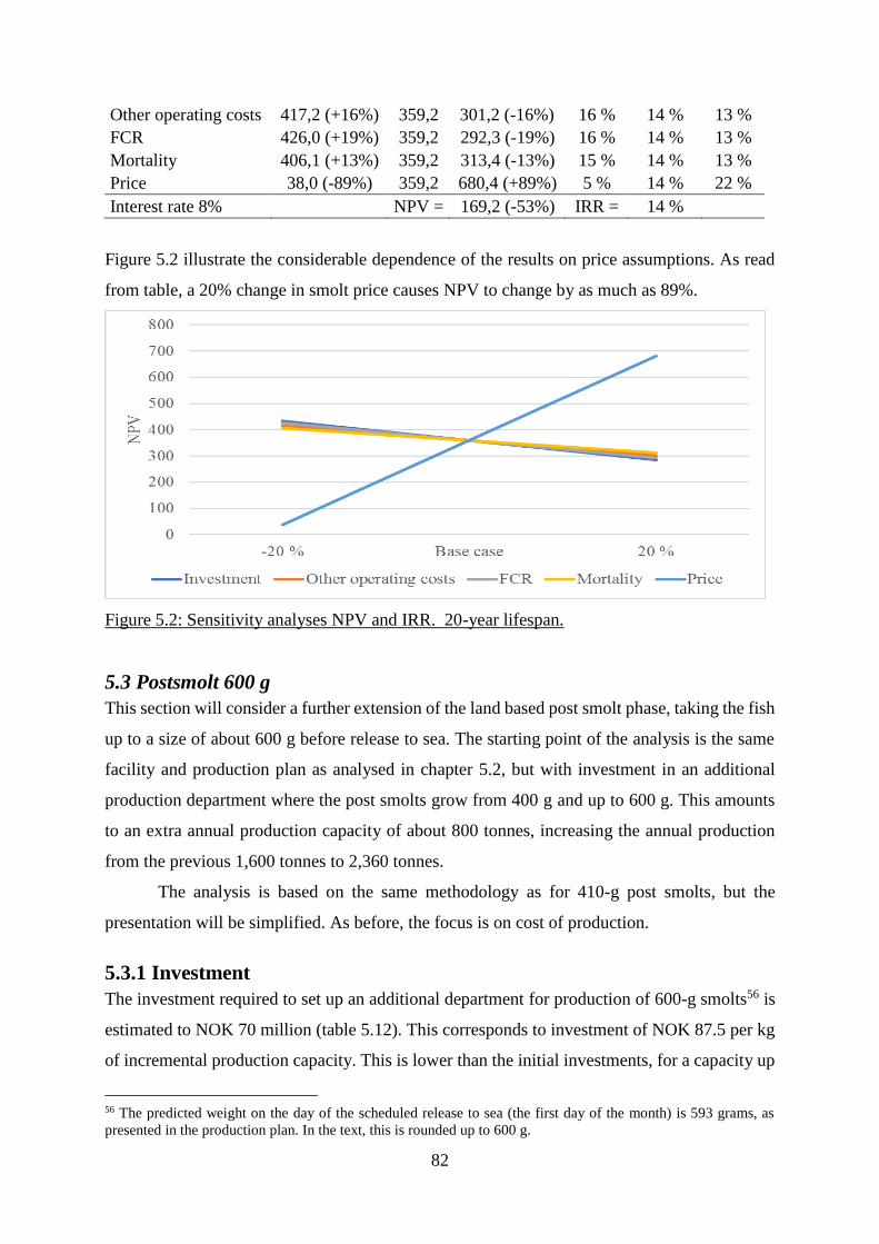
82

Other operating costs 417,2 (+16%) 359,2 301,2 (-16%) 16 % 14 % 13 %

FCR 426,0 (+19%) 359,2 292,3 (-19%) 16 % 14 % 13 %

Mortality 406,1 (+13%) 359,2 313,4 (-13%) 15 % 14 % 13 %

Price 38,0 (-89%) 359,2 680,4 (+89%) 5 % 14 % 22 %

Interest rate 8% NPV = 169,2 (-53%) IRR = 14 %

Figure 5.2 illustrate the considerable dependence of the results on price assumptions. As read

from table, a 20% change in smolt price causes NPV to change by as much as 89%.

Figure 5.2: Sensitivity analyses NPV and IRR. 20-year lifespan.

5.3 Postsmolt 600 g

This section will consider a further extension of the land based post smolt phase, taking the fish

up to a size of about 600 g before release to sea. The starting point of the analysis is the same

facility and production plan as analysed in chapter 5.2, but with investment in an additional

production department where the post smolts grow from 400 g and up to 600 g. This amounts

to an extra annual production capacity of about 800 tonnes, increasing the annual production

from the previous 1,600 tonnes to 2,360 tonnes.

The analysis is based on the same methodology as for 410-g post smolts, but the

presentation will be simplified. As before, the focus is on cost of production.

5.3.1 Investment

The investment required to set up an additional department for production of 600-g smolts56 is

estimated to NOK 70 million (table 5.12). This corresponds to investment of NOK 87.5 per kg

of incremental production capacity. This is lower than the initial investments, for a capacity up

56 The predicted weight on the day of the scheduled release to sea (the first day of the month) is 593 grams, as

presented in the production plan. In the text, this is rounded up to 600 g.

83

to 1,600 tonnes, indicating the possible existence of economies of scale. The investment is

based on a department consisting of three additional production tanks, each with a diameter of

16 m and based on a fish density of 70 kg per m3. It must be added that in practice, the division

into departments would have to be adapted for the production facility as a whole. This is due to

retention times within each department; these must be similar to secure flow and capacity

utilisation of the facility as a whole57.

With the added extension of the facility, total investments are up from NOK 350.4

million in the 400-g base case to NOK 420.4 million based on 600-g post smolt. Annual

depreciation and interest are now NOK 31.7 million (table 5.12). With the increased annual

production capacity, investment amounts to NOK 175.2 per kg of annual smolt production

capacity or NOK 105.6 per fish. This compares to NOK 219 per kg of annual smolt production

capacity or NOK 88 per fish in the 400-g base case.

Table 5.12: Investments in a 1,600 tonnes postsmolt facility. NOK ‘000.

Investment NOK ('000) Economic

lifetime

Depreciation

and interest

Total investment, base case (410 g) 350,377 26,523.9

600-g department 70,000 20 5,151.7

Total investment, 600-g production facility 420,377 31,674.7

5.3.2 Production plan

The production plan for the 600-g case is precisely the same as for 410-g smolts up to the point

of release to sea. However, in this case the fish are held for an additional month in the new

department upon reaching a size of 410 g, instead of being released to sea (see table 5.13). Thus,

only the last row of the production plan for a batch of smolts need to be changed. As the table

shows, the number of fish delivered to sea is slightly reduced as a consequence of an additional

month of mortality.

Table 5.13: Production plan for one batch

Month

(beginning) Department

Weight (g)

per fish, wt

Weight (g)

increase,

wt+1 – wt

Survival % Number of

fish, Nt

0 1 0,2 0,6 0,960 1 084 287

1 1 0,8 2,3 0,995 1 040 915

57 Otherwise, the fish would stay only for a very short time in the last department, so that this part of the facility

would be empty much of the time. This is not realistic, so in practice the division into departments would be

different. Alternatively, the last department could be designed to keep the fish up to a larger size – for on-growing

for the same time period as it takes for the next batch of fish to be ready to be released into the department.

84

2 1 3,1 4,9 0,995 1 035 711

3 2 8,0 16,0 0,995 1 030 532

4 2 24 26,0 0,995 1 025 379

5 2 50 42,0 0,995 1 020 253

6 3 92 73,1 0,995 1 015 151

7 3 165 104,2 0,995 1 010 076

8 4 269 140,9 0,995 1 005 025

9 4 410 183 0,995 1 000 000

10 5 593 995 000

A production plan is given in table 5.14 with cost assumptions in table 5.15. The tables

illustrate changes and adjustments to the ones above for 410-g smolts. Assumptions that are left

out from the tables remain as before.

Table 5.14: Production plan

Annual production 3.98 million post smolts per year, each of 593 grams. Total land

based production capacity equivalent to 2,360 tonnes

Number of fry/post

smolt for delivery Four deliveries to sea per year; 995,000 fish per delivery


2,153,555

Feed price NOK 15 per kg (range NOK 13-17 depending on contents)

Table 5.15: Cost assumptions:

Variable costs Change

Number of man-years 7 +1

Electricity

NOK 1 per kwh. (including “network rental fee” and “electricity fee”. 6

kwh per kg of production

14.4 million kWh per annum

Oxygen NOK 2.50 per kg. 1,200 tonnes per annum (0.5 kg per kg of production)

Oxygen storage tank rental: NOK 100-200 000 per annum

Water 0,4 m3 fresh water per minute. NOK 1.5 million per yeara)

Waste/wastewater NOK 800 per tonne (range NOK 130-2,000). 3,230 tonnes per annum

(1.5 kg per kg of feed, not dried)

Service, maintenance

and repairs

NOK 2 million per annum; range 1-2 million

+0.5 mill.

Other costs NOK 4 million +0.8 mill.

a) The consumption of fresh water is left unchanged. The selection of water sources

and related costs are as mentioned not straightforward. In this case, it is assumed

that the facility has both a freshwater and a seawater source, with freshwater

primarily in the initial phases (<80-100 g). After that, salt water is the dominant

water source, so that the cost of water consists primarily of energy costs.


In table 5.16 we present total annual cost for the 600-g smolt production, assuming steady state.

We also give average cost of productionper smolt and, for comparison, also for 410-g smolt.

85

The cost structures are fairly similar, but variable costs (70%) represent a slightly higher share

than before at the expense of a slightly lower cost share for fixed costs (30%).

Table 5.16. Cost of production for an annual production capacity of 4 million post smolts. Cost

of production per fish. NOK.

600-g smolt 410-g smolt

Total

cost NOK/ fish % of total NOK/ fish % of total

Feed 32 303 8,1 28 % 5,6 24%

Roe 4 819 1,2 4 % 1,2 5%

Vaccines 7 327 1,8 6 % 1,8 8%

Labour 4 655 1,2 4 % 1,0 4%

Insurance fisha) 1 943 0,5 2 % 0.4 2%

Other operating costs 28 606 7,2 25 % 5.2 23%

Interest on working

capitalb) 1 526 0,4 1 % 0.3 1%

Sum variable costs 81 179 20,4 70 % 15.5 67 %

Interest and

Depreciation 31 675 8,0 27 % 6.6 29%

Insurance on building and

equipmentc) 647 0,2 1 % 0,1 1%

Management 2 925 0,7 3 % 0,7 3%

Sum fixed costs 35 247 8,9 30 % 7.5 33 %

Total production cost 116 426 29,3 100 % 23.0 100%

Production cost per g 0.049 0.056

a) Insurance premium on fish is estimated over an annual, steady state production period

on the basis of all variable costs incurred in order to raise the fish (roe, feed, vaccines,

labour and other operating costs).

d) Interest on working capital is, as before, estimated based on feed, roe, vaccines, labour,

other operating costs, insurance and management costs.

b) For simplicity, it is assumed that half of the investment in the 600-g department is

related to building and half to equipment in the calculation of insurance cost.

Cost of production for a 600-g smolt is NOK 29.30 compared to NOK 23.00 for a 410-

g smolt, i.e., a difference of NOK 6.30, or 27.4% higher. This is mainly due to higher feed costs

(NOK 2.50), operating costs (NOK 2.00) and interest and depreciation (NOK 1.40) per fish.

Notwithstanding the increase in weight per fish, the production in terms of number of fish is

not increased in this case. So, when cost and investment increase, so does the cost of production

per fish.

5.4 Summary

This chapter has indicated that investments in production of post smolt may be a profitable

investment and that economies of scale might exist in larger post smolt facilities. In terms of

cost of production, it is estimated that the cost of a 410-g post smolt could amount to about

86

NOK 23 per fish. This corresponds to a cost of production per kg of NOK 56. Although there

are few references readily available for comparison, information is available on the estimated

cost of production for a 419-g smolt for a company in the Faroe Islands in 2013/14, which was

NOK 19.95 per fish, corresponding to NOK 47.6 per kg (in 2013/14 prices) (Kverneland, 2016).

The cost of a 600-g smolt in the current analysis is estimated to NOK 29.3, which would

correspond to a cost of production of 49.4/kg. Berget (2016) estimated cost of production per

kg for 650-g smolts to NOK 49.15/kg, which would be equivalent to 31.9 per fish. The

similarities between these few estimates and those of the current study are almost surprising

given the uncertainty associated with the data. Berget (2016) also estimated cost of production

of 1-kg post smolt, at NOK 42.6 per kg and per fish.

Table 5.17: Comparison of estimated cost of production from other studies and sources and the

current study. 400-g, 600-g, and 1,000-g smolts.

400-g 600-g 1,000-g

Per fish Per kg Per fish Per kg Per fish

This study 23.0 56.0 29.3 49.4 -

Berget (2016) - - 29.4a) 49.2 42.6

Industry source 26.5 64.6 36.0 60 56

Hiddenfjord

2013/14

19.95b) 47.6 - - -

a) Based on the cost of production per gram of a 650-g smolt – transformed to 600-g (by

dividing by 650 and multiplying by 600).

b) 419-g smolt in 2013/14.

As noted, approximate estimates have also been obtained from industry sources –

indicating own production costs around NOK 11 for a 100-g smolt, with additional increases

of about NOK 0.05 per additional gram over that. By this estimate, cost of production per fish

would be NOK 26.5 for a 410-g smolt and NOK 36.0 for a 600-g smolt. It is worthwhile to note

that the last estimate conflicts somewhat with the above indications in terms the degree of

linearity in cost accumulation. This estimate is a lot more conservative in terms of reduction in

cost per kg of larger fish (see table 5.17). As the table shows, it may also be that the estimated

cost of production is a bit low in this study, at least when compared to the industry source.

All studies imply a decreasing cost per kg as the smolts are grown to larger sizes on

land, but the assumptions about how significant the reduction in cost per kg might be, differ.

Thus, it is not clear how the cost of production can be expected to develop with increasing sizes

of smolt. It was emphasised in chapter II that considerable variations seem to exist in terms of

smolt producers’ facilities and technology, as companies in the industry have become

87

increasingly heterogeneous over time (Sandvold & Tveterås, 2014). Cost of production might

vary between both new and existing firms. With the data collected for this study, it is therefore

impossible to indicate or believe anything about the representativeness of the assumptions and

results.

Either way, the big question of interest to the salmon industry is neither the smolt price,

operating margin or cost of production in post smolt operations. Instead, the motivation for

investing in post smolt extends to its role and impact on the overall cost of production and

associated production risks. During the land based phase, the risks may presumably be shifted

to some extent from factors outside of the farmers control – to more internal, manageable and

controllable production risks. Moreover, increased smolt size is likely to reduce the grow-out

period in sea substantially. The potential increase in control of central growth parameters such

as temperature in land based facilities may also lead to a shortening of the overall production

time. In effect, many of the industry’s current challenges might be eased by a transition to post

smolt. However, according to some, the potential for increases in production turnover, capacity

utilisation and overall increases in production would be the ultimate prize (Holm et al. 2015).

In the following chapter, the analysis of land based post smolt production is extended

to looking at the sea based production phase, where the above mentioned and other points will

be addressed – with emphasis on cost of production and production planning with use of post

smolts.

88

VI THE GROW-OUT PHASE

In this chapter, we will analyse cost of production for the grow-out phase in sea, based on post

smolts. The chapter is focused on cost of production and will explore whether and how the

benefits of larger smolts and shorter production cycles may translate into economic advantages

in cost of production. The analysis is less extensive than before, taking official statistics on the

industry’s current cost of production as its point of departure. For this reason, it should be noted

that the analysis serves as a preliminary study and that it has some weaknesses. The cost

categories given by official statistics are aggregated and involve several sub-components for

which we do not have complete information about how they are incurred. For this reason, the

assumptions made about potential effects on cost of production by a transition to post smolt are

somewhat hypothetical. Nevertheless, the approach is effective in illustrating some important

points. In essence, it serves as a preliminary indication as to where and how potential benefits

and savings may be materialised – and the costs they need to weigh up for.

Cost of production will be analysed based on 410-g and 600-g post smolts, respectively.

In addition to the preliminary study of cost of production, a simple grow-out simulation is

carried out to examine the potential effects on production turnover, quantity and license

utilisation following a transition from 100-g to 410-g smolts.

As emphasised before, the production cycle can be considerably shorter when using

larger smolts. This gives rise to the previously discussed benefits of lower production risk,

shorter time between fallowing of production sites and less exposure of the fish to sea lice and

lice treatments. Sea lice and diseases will have shorter time to accumulate before a site is

emptied, and infected fish may be harvested instead of receiving treatments, as the fish sooner

will have reached desirable harvest weights. Some indications also exist that the mortality rate

may be lower in post smolt grow-out than among traditional 100-g smolts. For instance,

Mathisen (2016) presented experience with smolt and post smolt mortality in sea for various

sizes of smolt in the county of Finnmark, Norway in September 2014. The results indicated

lower rates of mortality and less variation in mortality rates among the larger smolts.

In general, however, enough knowledge has not been obtained to suggest a specific

difference in mortality rates between the two smolt sizes. The mortality assumption in this

chapter will be 0.75% per month in the grow-out simulations; 10% over 13 months by use of

410-g post smolt and 9.2% over 12 months by use of 600-g smolts. A mortality rate of 0.75%

89

per month is consistent with the assumption made by Dahl & Idsøe, but is low compared to the

current Norwegian mortality rate in sea58.

In the following, chapter 6.1, will consider cost of production based on 410-g post smolt

while we look at 600 g post smolt in chapter 6.2. One of the most disputed potential benefits of

large smolt – namely increased license utilisation and production increases – will be the subject

of a separate discussion in chapter 6.3, where production planning and the use of post smolts

under the MTB regime will be analysed briefly.

6.1 Cost of production – based on 410 g post smolt

The post smolt analysis will now be extended to explore grow-out of 410-gram post smolt in

sea-pens, using the same logic as before to analyse cost of production. Beside the size of smolts

released, the production process and annual cost of production in grow-out of 410-g smolts is

very much similar to the annual cost of production in operations using 100-g smolts. For this

reason, the analysis is simplified by use of available data from the Norwegian Directorate of

Fisheries. It might be argued that this is as good an estimate as any.

Nevertheless, some corrections must be made to account for the differences – most

importantly to smolt price. However, it is also of interest to examine the potential effects that

could be realised if the use of post smolts could enable farmers to increase production turnover

and thereby increase production quantity accordingly. Moreover, the elimination of several

months per production cycle is believed to reduce lice related costs. To examine the possible

effects of these benefits on cost of production, some hypothetical corrections to the official

statistics are undertaken.

First, the lengths of the respective production cycles are estimated, by use of post smolt

and traditional smolt, respectively. There are two reasons for this: First, there is the potential of

reducing the exposure time and accumulation period for sea lice. Second, it is of interest to

explore the potential effects of increased turnover in production, provided that a new generation

can be released upon harvest of another. The greatest result of such a possibility would be the

potential increase in sales and revenues. However, it is also worthwhile to consider the potential

gains in terms of cost of production – that is, any “economies of scale” that may exist when

fixed and/or indirect costs are distributed over a larger quantity of production.

58 After a positive development in 2012-13 with mortality of about 13-14%, the situation has worsened since then,

reaching 20% in 2016 (Hjeltnes et al. 2017). For comparison, the mortality in Faroe Islands is 10% (Hjeltnes et

al. 2017; kyst.no, 2017b).

90

Given assumptions as described under general assumptions in chapter IV, table 6.1

shows the production time from release of 410 g post smolts in month 0 to harvest of 5 kg

salmon in month 1359.

Table 6.1: Production time from release to sea until harvest, 410-g smolts

Month

(beginning)

Weight

(g) per

fish

0 410

1 517

2 680

3 879

4 1 101

5 1 361

6 1 664

7 1 985

8 2 352

9 2 769

10 3 210

11 3 713

12 4 285

13 5 000

In comparison, the production time using 100-g smolts is estimated to take about four

months more, with harvest in month 17. As emphasised before, the long production cycle means

that the fish will be exposed twice either to the unfavourable periods of the lowest temperatures

and the slowest growth or to the unfavourable periods with the highest risk of sea lice infection.

The traditional pattern of 100-g smolt release is highly seasonal with two annual peaks in May

and September-October, when most fish are transferred to sea. Using the same procedure and

assumptions as described above, figure 6.1 shows the expected weight curve for the two typical

releases. As illustrated, there is quite a large discrepancy in the time required to reach a

harvestable size of 5 kg. For simplification, it is assumed that harvest of 5-kg fish takes place

in month 17, which lie between the expectation for the May release and the October release,

respectively60.

59 See appendix, table C4 for details. The weight curve is based on the average of four annual releases with dates

of release as given by the land based operations above (December, March, June and September). As the appendix

shows, the average weight at the beginning of month 13 is 4,889 g. For simplification, the production time has

been rounded off to 13 months. 60 The weight curves for May and October are given in appendix, table C5a.

91

Figure 6.1: Production time from release to harvest, 100-g smolts. Releases in May and October,

respectively.

From official statistics from the Norwegian Directorate of Fisheries, we have the current

cost of production per kg (see table 2.1, chapter II). Taking this as our starting point,

adjustments will be made to account for the difference in production time and potentially

quantity by use of 410-g post smolts. In doing so, the most important distinction is between

costs that are incurred directly in relation to production and fish growth such as feed, compared

to other cost categories such as labour, administration and certain other costs that are less

closely tied to the quantity produced. The assumption is that these costs will remain

approximately at the same level year-on-year, regardless if a production cycle is completed in

13 or in 17 months. Hence, if a production cycle could be completed in 13 rather than 17

months, the labour cost per kg could be reduced to 13/17 of the current cost per kg. A few

conditions are necessary for this to be realised. Importantly, the capacity which is freed up must

either be utilised for production (i.e., increasing the production turnover so that in three years,

four cycles could be completed instead of three) or eliminated (which is conceivably only an

option in the case of labour); here, the former option is our preliminary assumption.

Nevertheless, it must be noted that a major issue in this respect is the limitations imposed

by the MTB regime, which dictate an absolute biomass limit both at the level of a location and

at the level of the company. We shall disregard this for now and analyse the matter further in

section 6.3 below. It can, however, be added that what is assumed here is the maximum

conceivable increase in turnover and production resulting from a transition from 100 to 410-g

smolts61.

61 The number of months of fallowing between production cycles is assumed to be the same – i.e., two months –

after harvest of a generation with either size of smolts. However, over time the number of fallowing months is

larger when (only) post smolts are used, as it happens more frequently.

92

It may, anyway, still not be sufficient to correct cost of production for the difference in

production time alone. As the production costs are given per kg of production, it is also

appropriate to take account of the fact that for one 5-kg salmon, the produced quantity differs

depending on whether 100-gram or 410-gram smolts are released (4.9 kg versus 4.59 kg,

respectively). The difference of 310 g would amount to 6.3% of an individual harvest weight

of 5 kg, which is not negligible. For this reason, the adjusted components of 410-g cost of

production per kg will be multiplied by a factor of 1.063 to account for a lower quantity

produced per cycle, in addition to the factor 13/17 to account for a shorter production cycle as

described above62.

To determine which of the cost components that should be adjusted for differences in

production time and quantity produced, we must separate between the costs that are fixed or

indirect and thus likely to be constant within the relevant production range – and those that

relate directly to the production quantity, such as feed and smolts. In addition to the distinction

between more and less direct costs of production per kg, two other important items require

attention when estimating cost of production based on official statistics – namely smolt cost

and interest on license values. Both will be addressed in the following. The cost of production

by use of the two production modes is illustrated and compared in table 6.2. Apart from interest

and depreciation, the first column is identical to the actual cost statistics for traditional salmon

aquaculture as presented in chapter II (table 2.1).

In the official statistics, cost figures per kg contain a certain mortality. As noted above,

data on how this may differ over a production cycle and how this may affect the cost of

production between the two methods has not been obtained. Smaller smolts and a longer

production cycle increases the risk of losses in all phases of the cycle, including for large fish.

As mentioned in chapter II, challenges with sea lice have recently led to both reductions in

average harvest weight and losses of large fish, both of which lower the final quantity produced

and increases the cost of production per kg. Since our estimated 410-g cost of production takes

official statistics as its point of departure, we may keep in mind that these could incorporate

part of the costs they are supposed to eliminate. In the following, we will examine the possible

savings in de-licing costs separately by making assumptions about potential reduction in “other

costs”.

62 Official statistics define production quantity as: (Quantity sold + frozen stock) + ((live stock 31.12. – weight of

smolt released – live stock 1.1.) /1,067), where 1.067 is the conversion rate from live weight to WFE.

93

Table 6.2: Cost of production production per kg. Traditional farming based on 100 g smolts

(2015) and 410-g post smolt (estimate). NOK/kg.

Traditional farminga)

(2015),

100-g smolts

Cost based on 410-g

post smolt

Smolt cost 2,72 10 % 7,19 24 %

Feed cost 13,18 46 % 13,18 44 %

Insurance 0,13 0 % 0,13 0 %

Labour 2,07 7 % 1,68 6 %

Other operating costs 6,31 22 % 4,31 14 %

Sum variable costs 24,41 86 % 26,49 89 %

Depreciation 1,58 6 % 1,28 4 %

Financial costs 0,16 1 % 0,16 1 %

Interest on license value 2,39 8 % 1,94 7 %

Sum fixed costs 4,13 14 % 3,39 11 %

Total production cost 28,54 100 % 29,88 100 %

a) With own estimates for interest on licenses.

Source for traditional farming: The Norwegian Directorate of Fisheries

Like before, we assume the price of a 410-g smolt is NOK 30.00 (table 5.6). If one smolt

results in one 5-kg salmon, this corresponds to a smolt cost of NOK 6.54 per kg produced63. A

question in this respect is whether the cost should be distributed over the full harvest weight or

only the quantity actually being produced in sea, i.e., taking account of the size of smolts

released. In the official statistics, the quantity produced includes a correction for the size of

smolts released, and for this reason it seems appropriate to do the same here (return to footnote

66 above for information). Thus, the quantity produced per 5-kg salmon is 4.59 kg after

subtracting the smolt weight. However, it must be noted that this makes it increasingly

challenging to weigh up for the higher price of post smolt – the larger the smolts are, the higher

the smolt price and the lower the production quantity it is distributed over. It could very well

be discussed whether this is the appropriate way to do this. It must also be corrected for

mortality during grow-out. If we set this at 10%, the “real cost” per smolt becomes NOK 33 or

NOK 7.16 per kg.

Feed cost per kg is determined by the price per kg of feed and the economic FCR (i.e.,

biological FCR corrected for feed waste and mortality). As noted above, data on the pattern of

mortality over the 100-g and 410-g grow-out cycles has not been obtained. Moreover, while the

biological FCR is sometimes assumed to be lower and more efficient in smaller fish (ref. chapter

IV and V land based), the feed price and mortality may be higher in the period between 100 g

63 This number has taken account of the smolt weight, i.e., assuming a production per 5-kg fish of 5,000 g – 410 g

= 4,590 g.

94

and 410 g. The net effect in terms of differences in feed cost per kg in grow-out of 100-g versus

400-g smolt is not necessarily clear-cut, so it may be as appropriate to assume the same feed

cost per kg of production in both cases. For this reason, the feed cost of NOK 13,18 per kg is

assumed to remain the same in 410-g grow-out. However, if considerable losses of large salmon

can be eliminated or reduced by use of larger smolts, then the feed cost per kg should be lower.

In terms of insurance cost, the official statistics do not provide distinctions between

insurance on fish stock and insurance on equipment. Thus, the figure may include both. Since

investments in physical structures and equipment tend to be relatively moderate in sea based

production, insurance of fish stock may constitute a major share of the given insurance cost.

For that reason, no correction is made to insurance cost per kg.

For other operating costs, estimates indicate that current costs associated with lice

prevention, control and treatment amount to NOK 5/kg or more64. With production based on

410-g post smolt, the sea phase is reduced and issues related to lice should be lessened. As an

estimate, we assume this will lead to a reduction in other operating costs of NOK 2.00/kg

although it must be acknowledged that this is somewhat arbitrary.

When it comes to interest, based on the discussion in Chapter II, a valuation of NOK 80

million per permission is assumed. Also, as noted in chapter II, the average sales quantity

(WFE) per permission was 1,338 tonnes in 2015. With no depreciation on license values,

interest at 4% amounts to NOK 3.2 million per permission per year and NOK 2.39 per kg.

Financial cost is left unchanged. It is included here as a fixed cost, indicating that it

consists of interest on loans, but it may perhaps as well involve interest on working capital.

Wages as well as fixed costs (depreciation and the estimated interest on licence values)

are assumed to be incurred on an annual basis regardless of the production model used. For that

reason, the cost per kg is corrected for the expected difference in production time per cycle and

turnover between the two production modes. We approach this by multiplying the cost per kg

with 13/17 to account for the reduced production cycle and 1.063 to account for a lower

production quantity per fish due to the larger size of smolts.

In summary, the potential savings in cost of production per kg consist of savings in

indirect costs (wages) and capital costs (interest and depreciation) by cost distribution over a

larger quantity of output, as well as absolute cost savings in terms of reduction in de-licing cost.

Together, the three components amount to a difference of NOK 3.13 per kg compared to the

same components in the official statistics, which is equivalent to about 10% of the total 410-g

64 For completeness, it should be mentioned that the lice cost in the county of Finnmark is zero (chapter II).

95

cost of production per kg. The components are presented in table 6.3. As can be seen, the

majority of the assumed savings potential relates to a reduction in lice related cost. These, set

to NOK 2 on the basis of own judgement, make up two thirds of the total savings. Wages,

interest and depreciation together make up one third (whereof 0,39 in wage cost and 0,74 in

interest and depreciation). In comparison, the increase in smolt cost is about NOK 4.5 per kg.

Table 6.3 Potential savings in capacity costs per kg of production (as a result of increased

production and turnover).

Potential savings (NOK/kg)

Savings

(NOK/kg)

% of total

savings

Wages 0,39 12 %

Other costs (lice treatment) 2,00 64 %

Depreciation & interest 0,74 24 %

Total estimated saving 3,13 100 %

Share of total cost per kg 10%

The information to be drawn from this analysis is that the potential cost savings, here

estimated to about NOK 3/kg and primarily related to the cost of sea lice (NOK 2/kg), should

preferably make up for the increase in smolt cost. In this case, the increase in smolt cost per kg

is about NOK 4.50, and for this reason the total cost of production per kg is expected to increase

by about NOK 1.5 compared to the base case.65

While the reduction in de-licing cost is based on the elimination of four months in sea,

the estimates savings in fixed and indirect costs rely on the possibility of increasing production

(turnover). As noted, this assumption will be examined in detail in chapter 6.3.

6.2 Cost of production – based on 600-g post smolt

The analysis of cost of production in grow-out of 410-g smolts can be replicated, using the same

procedure and making equivalent assumptions, for the case of 600-g smolts (or 593 to be

precise). By use of the 593-g smolts, the production period is reduced to 12 months (compared

to 13 in the case of 410-g smolts). On the other hand, out of a harvest weight of 5 kg, the

quantity produced in sea is reduced to 4.4 kg. This reduction amounts to 493 g, equivalent to a

10,1% reduction in production per fish compared to the 100-g “base case”66.

65 That is assuming that the realisation of increased production turnover and economies of scale holds true. 66 Production in sea per 5-kg salmon harvested: 4.9 kg using 100-g smolts or 4.4 using 600-g smolts.

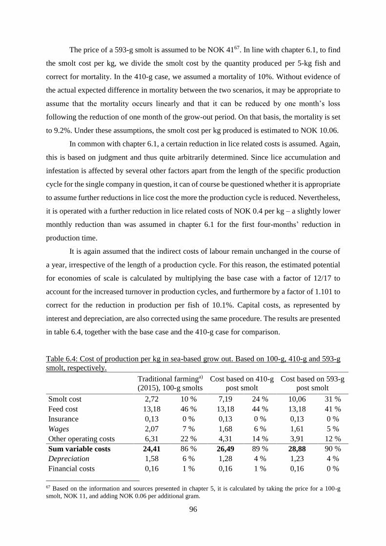
96

The price of a 593-g smolt is assumed to be NOK 4167. In line with chapter 6.1, to find

the smolt cost per kg, we divide the smolt cost by the quantity produced per 5-kg fish and

correct for mortality. In the 410-g case, we assumed a mortality of 10%. Without evidence of

the actual expected difference in mortality between the two scenarios, it may be appropriate to

assume that the mortality occurs linearly and that it can be reduced by one month’s loss

following the reduction of one month of the grow-out period. On that basis, the mortality is set

to 9.2%. Under these assumptions, the smolt cost per kg produced is estimated to NOK 10.06.

In common with chapter 6.1, a certain reduction in lice related costs is assumed. Again,

this is based on judgment and thus quite arbitrarily determined. Since lice accumulation and

infestation is affected by several other factors apart from the length of the specific production

cycle for the single company in question, it can of course be questioned whether it is appropriate

to assume further reductions in lice cost the more the production cycle is reduced. Nevertheless,

it is operated with a further reduction in lice related costs of NOK 0.4 per kg – a slightly lower

monthly reduction than was assumed in chapter 6.1 for the first four-months’ reduction in

production time.

It is again assumed that the indirect costs of labour remain unchanged in the course of

a year, irrespective of the length of a production cycle. For this reason, the estimated potential

for economies of scale is calculated by multiplying the base case with a factor of 12/17 to

account for the increased turnover in production cycles, and furthermore by a factor of 1.101 to

correct for the reduction in production per fish of 10.1%. Capital costs, as represented by

interest and depreciation, are also corrected using the same procedure. The results are presented

in table 6.4, together with the base case and the 410-g case for comparison.

Table 6.4: Cost of production per kg in sea-based grow out. Based on 100-g, 410-g and 593-g

smolt, respectively.

Traditional farminga)

(2015), 100-g smolts

Cost based on 410-g

post smolt

Cost based on 593-g

post smolt

Smolt cost 2,72 10 % 7,19 24 % 10,06 31 %

Feed cost 13,18 46 % 13,18 44 % 13,18 41 %

Insurance 0,13 0 % 0,13 0 % 0,13 0 %

Wages 2,07 7 % 1,68 6 % 1,61 5 %

Other operating costs 6,31 22 % 4,31 14 % 3,91 12 %

Sum variable costs 24,41 86 % 26,49 89 % 28,88 90 %

Depreciation 1,58 6 % 1,28 4 % 1,23 4 %

Financial costs 0,16 1 % 0,16 1 % 0,16 0 %

67 Based on the information and sources presented in chapter 5, it is calculated by taking the price for a 100-g

smolt, NOK 11, and adding NOK 0.06 per additional gram.

97

Interest on license value 2,39 8 % 1,94 7 % 1,86 6 %

Sum fixed costs 4,13 14 % 3,39 11 % 3,25 10 %

Total production cost 28,54 100 % 29,88 100 % 32,13 100 %

As revealed by the higher cost of production per kg, the increase in smolt cost per kg is

higher than the estimated savings in de-licing costs and the savings per kg from increased

turnover under the given assumptions. It is also worthwhile to note that the smolt cost has

increased to 31% of the cost of production, almost approaching the share of feed. In absolute

terms, the increase in smolt cost per kg from the base case to 593-g smolt is NOK 7.3.

Meanwhile, the potential savings per kg compared to traditional smolts are estimated to NOK

3.75, primarily related to reduction in lice cost (see table 6.5). As a result, the net effect on cost

of production per kg is an increase of about NOK 3.60 compared to the base case.

Table 6.5 Potential savings

Potential savings (NOK/kg) - compared to "base

case"

Savings

(NOK/kg)

% of

saving

Wages 0,46 12 %

Other costs (lice treatment) 2,4 64 %

Depreciation & interest 0,88 24 %

Total est. saving 3,75 100 %

Share of total cost per kg 12 %

6.3 Production planning and the use of post smolt under the MTB regime

This section will elaborate further on some key issues in sea-based production and production

planning in Norway, comparing releases of 100-g smolts and post smolts of 410-g. The aim of

the study is to explore and illustrate possible differences and similarities in how the MTB-

regime influences production planning in both production modes. The question is whether and

how the introduction of larger smolts may affect the amount of harvest a farm is able to achieve

for a given MTB. As emphasised in this chapter, this potential has implications not only for the

ability to generate additional revenue, but also for the possibility of distributing costs over a

larger production quantity. Such a possibility would increase cost competitiveness and

contribute to make up for a higher smolt cost and the likely increase in cost of production by

use of post smolt.

Although considerable increases in production and harvest quantity for a given MTB

resulting from transition to post smolt is suggested by some (Holm et. al, 2015; Kyst.no, 2017c;

Ilaks.no, 2015; Nofima, n.d.; Rådgivende biologer, 2016), it is questioned by others (Mathisen,

98

F., 2016). Because of the MTB design, it may be the case that for companies that already have

their biomass continuously adjusted close to the MTB-limit, the possibility to take out any extra

production by use of post smolt is negligible or non-existent. To shed light on this question,

two separate production planning simulations will be presented. Under similar assumptions, the

analysis is carried out using 100-g and 410-g smolts, respectively. The study is based on a

production planning design as presented by Dahl & Idsøe (2017). First, a model is established

using 410-g post smolts and data as presented previously. Thereafter, a similar analysis is

presented using 100-g smolts.

The Norwegian regulation regime was presented briefly in chapter II. As noted, both

permissions and locations are required to establish aquaculture operations. A permission is

often allowed to be connected to up to four to six locations, so as to enable the farmers to have

flexible production throughout the year (Guttelvik, O.B., 2014). The traditional production

cycle for one location is to release smolts of 50-100 g with harvest of 4-5 kg salmon (ibid.). A

production cycle at a location under these assumptions consists of about 15-24 months of grow-

out followed by two months of fallowing.

In the county of Møre og Romsdal, many locations have a production limit of 3,120-

4,680 tonnes MTB, as determined by environmental considerations (Guttelvik, O.B., 2014).

The complexity of the farmers’ production planning problem appears when the farmer not only

has to stay within their total biomass cap as given by their number of permissions (the company-

level MTB), but must also ensure that their production at no time exceeds the MTB for any

single location. A location with an MTB of 3,120 tonnes MTB could for instance contain over

a million 3-kg individuals, but only about 600,000 if the weight is 5 kg. To maximise output

and achieve a satisfactory MTB-utilisation, farmers depend on having enough flexibility in their

production and enough locations to enable the company-level biomass to remain as close as

possible to the company-level MTB at all times, without ever exceeding it.

It has been noted that one of the potential benefits of larger smolts is that more robust

fish and a shorter cycle may enable farmers to maintain a larger, more stable production by

increasing the turnover and number of generations released and harvested throughout the year.

The larger fish may also overcome some of the challenges imposed by long growth cycles and

the highly seasonal variations in sea temperature and disease related conditions. Although the

exact effect of post smolts and a shorter sea phase remains uncertain until actual experience

with large-scale grow-out of generations of fish provides evidence of it, figure 6.2 illustrates

the expected development in individual fish weights for each possible month of release of post

smolts within a year, i.e., January – December. As illustrated, simulations based on previously

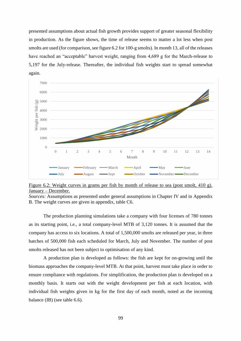
99

presented assumptions about actual fish growth provides support of greater seasonal flexibility

in production. As the figure shows, the time of release seems to matter a lot less when post

smolts are used (for comparison, see figure 6.2 for 100-g smolts). In month 13, all of the releases

have reached an “acceptable” harvest weight, ranging from 4,689 g for the March-release to

5,197 for the July-release. Thereafter, the individual fish weights start to spread somewhat

again.

Figure 6.2: Weight curves in grams per fish by month of release to sea (post smolt, 410 g).

January – December.

Sources: Assumptions as presented under general assumptions in Chapter IV and in Appendix

B. The weight curves are given in appendix, table C6.

The production planning simulations take a company with four licenses of 780 tonnes

as its starting point, i.e., a total company-level MTB of 3,120 tonnes. It is assumed that the

company has access to six locations. A total of 1,500,000 smolts are released per year, in three

batches of 500,000 fish each scheduled for March, July and November. The number of post

smolts released has not been subject to optimisation of any kind.

A production plan is developed as follows: the fish are kept for on-growing until the

biomass approaches the company-level MTB. At that point, harvest must take place in order to

ensure compliance with regulations. For simplification, the production plan is developed on a

monthly basis. It starts out with the weight development per fish at each location, with

individual fish weights given in kg for the first day of each month, noted as the incoming

balance (IB) (see table 6.6).

0

1000

2000

3000

4000

5000

6000

7000

0 1 2 3 4 5 6 7 8 9 10 11 12 13 14

Wei

ght

per

fis

h (

g)

Month

January February March April May June

July August Sept October November December

100

Table 6.6: Weight curves of individual fish weight per location

Month

(IB) Location 1 Location 2 Location 3 Location 4 Location 5 Location 6

Weight per fish (kg) Mar 0,410 Apr 0,473 May 0,594 Jun 0,785 Jul 1,078 0,410 Aug 1,486 0,587 Sept 1,970 0,857 Oct 2,455 1,142 Nov 2,893 1,409 0,410 Dec 3,310 1,670 0,505 Jan 3,645 1,884 0,603 Feb 3,976 2,099 0,705 Mar 4,327 2,329 0,818 0,410 Apr 4,689 2,571 0,940 0,473 May 5,227 2,934 1,130 0,594 Jun 6,002 3,467 1,417 0,785 Jul 7,079 4,222 1,843 1,078 0,410

Aug 8,439 5,197 2,416 1,486 0,587 Sept 6,276 3,076 1,970 0,857 Oct 7,301 3,722 2,455 1,142 Nov 8,191 4,295 2,893 1,409 0,410

Dec 9,015 4,836 3,310 1,670 0,505

Jan 5,265 3,645 1,884 0,603

Feb 5,687 3,976 2,099 0,705

Mar 0,410 6,130 4,327 2,329 0,818

Apr 0,473 6,586 4,689 2,571 0,940

May 0,594 5,227 2,934 1,130

Jun 0,785 6,002 3,467 1,417

Jul 1,078 0,410 7,079 4,222 1,843

Aug 1,486 0,587 8,439 5,197 2,416

Sept 1,970 0,857 6,276 3,076

Oct 2,455 1,142 7,301 3,722

Nov 2,893 1,409 0,410 8,191 4,295

Dec 3,310 1,670 0,505 9,015 4,836

Jan 3,645 1,884 0,603 5,265

Feb 3,976 2,099 0,705 5,687

Mar 4,327 2,329 0,818 0,410 6,130

Apr 4,689 2,571 0,940 0,473 6,586

The monthly mortality rate is set to 0.75% and is assumed to be the same for all locations

and months. As discussed in section 6.1, some indications exist that the mortality rate may be

lower with post smolt than with regular smolts. However, there is scarce evidence as to how

101

large such a difference may be. For that reason, the following models and estimates use similar

mortality rates, with the only difference being a larger number of months with mortality in sea

for 100-g smolts. The monthly mortality rate, together with the harvest plan (in number of fish),

is the basis for determining the number of fish per site at any time. The number of fish is

estimated at the beginning of each month. At the end of the month, all fish either die, are

harvested or transferred to the beginning balance of next month. In table 6.7 below, the

development in number of fish for the first release(s) at each location is shown. The number of

fish at the start of each month is calculated as follows: Number of survived fish from the

previous month minus the mortality (in number of fish) and the number of harvested fish in the

previous month.68

Table 6.7: The development in number of fish per location (given by the survival rate and the

harvest quantity)

Release

per batch

Monthly

mortality

Month

(IB)

Loc.

1

Loc.

2

Loc.

3

Loc.

4

Loc.

5

Loc.

6

Number of fish (IB = IB Survived fish – previous month’s

harvest)

500 000 0.75% Mar 500 000

Apr 496 250

May 492 528

Jun 488 834

Jul 485 168 500 000

Aug 481 529 496 250

Sept 477 918 492 528

Oct 474 333 488 834

Nov 470 776 485 168 500 000

Dec 467 245 481 529 496 250

Jan 450 871 477 918 492 528

Feb 378 689 474 333 488 834

Mar 264 599 470 776 485 168 500 000

Apr 178 614 467 245 481 529 496 250

May 78 615 463 741 477 918 492 528

Jun 0 412 763 474 333 488 834

Jul 0 190 787 470 776 485 168 500 000

Aug 0 52 916 467 245 481 529 496 250

Sept 0 0 378 231 477 918 492 528

Oct

0 252 094 474 333 488 834

Nov

0 108 053 470 776 485 168 500 000 Dec

0 44 443 467 245 481 529 496 250

Jan

0 0 450 871 477 918 492 528 Feb

0 378 689 474 333 488 834

Mar 500 000

0 264 599 470 776 485 168

68 Regarding harvest quantity, only fish that would otherwise survive to the next month are harvested in this model.

102

Apr 496 250

0 178 614 467 245 481 529 May 492 528

0 78 615 463 741 477 918

Jun 488 834

0 412 763 474 333 Jul 485 168 500 000

0 190 787 470 776

Aug 481 529 496 250

0 52 916 467 245 Sept 477 918 492 528

0 0 378 231

From the start, the biomass budget is developed for the first two first releases per

location without any harvest. This allows us to calculate the development in company biomass

if no harvest is undertaken. As the table shows, a separate column keeps track of the incoming

biomass for each month. Although that is helpful, it is not sufficient under the MTB regime.

Even if we ensured that the biomass on the first day of each month was exactly at (or just

slightly below) the MTB of 3,120 tonnes, this would constitute a breach of the MTB rule at the

end of the month before harvest: equal to the entire month’s net growth (i.e., after mortality but

disregarding harvest). For this reason, a company that harvests fish each month (or periodically

according to some other defined period, such as per day, week, etc.) would ensure that at the

beginning of the period, the biomass is equal to the MTB minus the coming period’s net growth.

That way, on the day of harvest, forecasted biomass is exactly at the MTB limit – and the

company ensures regulatory compliance as well as MTB utilisation69. According to sources

within the industry, large companies can have production large and continuous enough to

maintain daily harvests of the net growth (industry source).

Following the reasoning above, table 6.8 incorporates a separate column for a “net

growth forecast” for each month. This again offers the opportunity to determine a “target IB

biomass”, which is equal to the MTB-limit less the month’s forecasted growth. To maintain full

control over the biomass situation compared to the target biomass, the fourth column is defined

as “target biomass – IB biomass”. When the budget shows that the company biomass, calculated

on a monthly basis as the sum of IB weight per fish times the IB number of fish across each of

the six locations, exceeds the target level, the IB biomass balance becomes negative and harvest

must be scheduled for the month prior to exceeding the MTB. The harvest quantity is adjusted

until the biomass balance reaches positive territory.

69 In theory, this may seem simple but in practice it is not likely so. For one thing, the net growth varies substantially

within a year – and can probably vary substantially between years and for all sorts of unpredictable reasons as

well. Moreover, the farmer has several other restraints to take account of: to name a few, harvest may for various

reasons be restricted to certain periods and to certain minimum and maximum quantities. In addition, harvest and

release may be affected by other rules or considerations such as coordinated fallowing which puts restrictions on

the flexibility of individual production plans.

103

It follows from this that we assume that the MTB at the location level is not a

constraining factor and therefore not becomes binding (i.e., that the maximum biomass allowed

per location is “generous” enough to never be exceeded for any of the single locations under

this production plan). This way, the focus is on overall production and company-level MTB.

In our example, the company-level biomass exceeds the target for the first time in

January, less than one year after the first release (table 6.8). To avoid exceeding the MTB per

January 1st, 12,870 fish are harvested in December (month end). Following this harvest, the

budget shows that to avoid exceeding the target MTB at February 1st, the harvest in January

must be about 68,800 fish, and so on. Harvest is, of course, always first taking place at the

location with the oldest and largest salmon.

Table 6.8: The development in company-level biomass and harvest per location.

Month

(IB)

IB

biomass

Net

growth

forecast

(NGF)

Target

IB

biomass

= MTB -

NGF

IB

biomass

balance

Loc

1

Loc

2

Loc

3

Loc

4

Loc

5

Loc

6

Harvest (number)

Mar 205 000 29 567 3 090

433 2 885 433 0 0 0 0 0 0

Apr 234 567 58 116 3 061

884 2 827 317 0 0 0 0 0 0

May 292 683 91 140 3 028

860 2 736 176 0 0 0 0 0 0

Jun 383 824 139 091 2 980

909 2 597 085 0 0 0 0 0 0

Jul 727 915 279 015 2 840

985 2 113 070 0 0 0 0 0 0

Aug 1 006 930 356 791 2 763

209 1 756 279 0 0 0 0 0 0

Sept 1 363 721 359 011 2 760

989 1 397 267 0 0 0 0 0 0

Oct 1 722 733 322 503 2 797

497 1 074 765 0 0 0 0 0 0

Nov 2 250 235 351 099 2 768

901 518 666 0 0 0 0 0 0

Dec 2 601 334 286 400 2 833

600 232 266 12 870 0 0 0 0 0

Jan 2 840 826 279 117 2 840

883 57 68 800 0 0 0 0 0

Feb 2 846 369 273 507 2 846

493 124 111 250 0 0 0 0 0

Mar 2 843 547 276 335 2 843

665 118 84 000 0 0 0 0 0

Apr 2 726 015 393 935 2 726

065 50 98 660 0 0 0 0 0

May 2 604 225 515 768 2 604

232 8 78 025 47 500 0 0 0 0

Jun 2 487 012 632 948 2 487

052 40 0 218 880 0 0 0 0

Jul 2 400 897 719 005 2 400

995 97 0 136 440 0 0 0 0

Aug 2 410 885 709 063 2 410

937 52 0 52 519 85 510 0 0 0

104

Sept 2 527 281 592 714 2 527

286 5 0 0 123 300 0 0 0

Oct 2 661 057 458 892 2 661

108 51 0 0 142 150 0 0 0

Nov 2 714 364 405 547 2 714

453 89 0 0 62 800 0 0 0

Dec 2 816 240 303 728 2 816

272 32 0 0 44 109 12 870 0 0

Jan 2 840 828 279 117 2 840

883 54 0 0 0 68 800 0 0

Feb 2 846 372 273 507 2 846

493 122 0 0 0 111 250 0 0

Mar 2 843 550 276 335 2 843

665 114 0 0 0 84 000 0 0

Apr 2 726 018 393 935 2 726

065 47 0 0 0 98 660 0 0

May 2 604 225 515 768 2 604

232 8 0 0 0 78 025 47 500 0

Jun 2 487 012 632 948 2 487

052 40 0 0 0 0 218 880 0

Jul 2 400 897 719 005 2 400

995 97 0 0 0 0 136 440 0

Aug 2 410 885 709 063 2 410

937 52 0 0 0 0 52 519 85 510

Sept 2 527 281 592 714 2 527

286 5 0 0 0 0 0 123 300

As can be seen from the tables above (see also appendix, table C7), steady state harvest

is maintained from January after the first harvest, when the company continues to follow the

same pattern of releases and harvests. Given this production plan, each location is scheduled to

lie fallow for at least nine months, with nine months of fallowing for the location with the

March-release and 10 months of fallowing of the locations with the two other releases.

In terms of production, the budget gives the expected harvest quantity under the

assumption that harvest occurs at the end of the month and only fish which survive until the

end of the month may be harvested. Harvest quantity in kg is calculated using the outgoing

balance (OB) weight per fish (i.e., IB next month) since, by the specifications of the model,

harvest is done at the end of the month. For the simulation above, the annual steady state harvest

is estimated to 6,175.55 tonnes at UB weight, corresponding to 1,543.89 tonnes per permission.

The average harvest weight is 4.5 kg (6,175.55 tonnes divided by 1,366,813 individuals of

harvested salmon). For comparison, the average production per license was 1,338 tonnes in

2015 (WFE, only salmon), i.e., 1,428 in live weight.

100-g smolts

We now turn to the same production planning problem in the case of 100-g smolts. Figure 6.3

illustrates the expected development in individual fish weights for 100-g smolts from the point

of release to sea, for each possible month of release within a year (January – December). After

12 months, when all of the fish have been exposed to each annual season regardless of the

105

month of release, the weight curves merge. However, whereas the post smolts already were

approaching harvestable weights at this point, the 100-g smolts have only reached sizes ranging

from 2.393 kg – 2.463 kg. After this point, the weight development spreads again, with growth

rates dependent on the temperatures expected in the following months of grow-out. As the

figure reveals, the month of release matters a lot more in this case than for 410-g smolts. In

months 17-18, all releases have reached an “acceptable” harvest weight, but the weight range

is wide: between 4.059 kg (for the December-release) and 6.353 (for the May-release) in month

17 and between 4.553 kg (for the November-release) and 7.166 (for the May-release) in month

18.

Figure 6.3: Weight curves in grams per fish by month of release to sea (100-g smolt). January

– December. (See appendix, table C5b for details.)

As before, we consider a company with six locations and in possession of four 780-

tonne licenses, i.e., a total company-level MTB of 3,120 tonnes. The smolt quantity is also the

same as before: 1,500,000 smolts per annum in three batches of 500,000 smolts each with

releases again scheduled for March, July and November. The fish are kept for on-growing until

the biomass approaches the targeted company-level biomass and harvest must be undertaken in

order to comply with the MTB.

Given the assumptions stated, the annual steady state harvest is estimated at 5,958

tonnes at Outgoing Balance (OB) weight compared to 6,176 tonnes using 410-g smolts as

summarised in table 6.9. This corresponds to 1,489 tonnes per permission (compared to 1,544

tonnes per permission using 410-g smolts). The average harvest weight is 4.5 kg (5,958 tonnes

divided by 1,328,760 individuals of harvested salmon). After the last round of harvests per

0

1000

2000

3000

4000

5000

6000

7000

8000

9000

0 1 2 3 4 5 6 7 8 9 10 11 12 13 14 15 16 17 18 19

Wei

ght

per

fis

h (

g)

Month

January February March April May June

July August Sept October November December

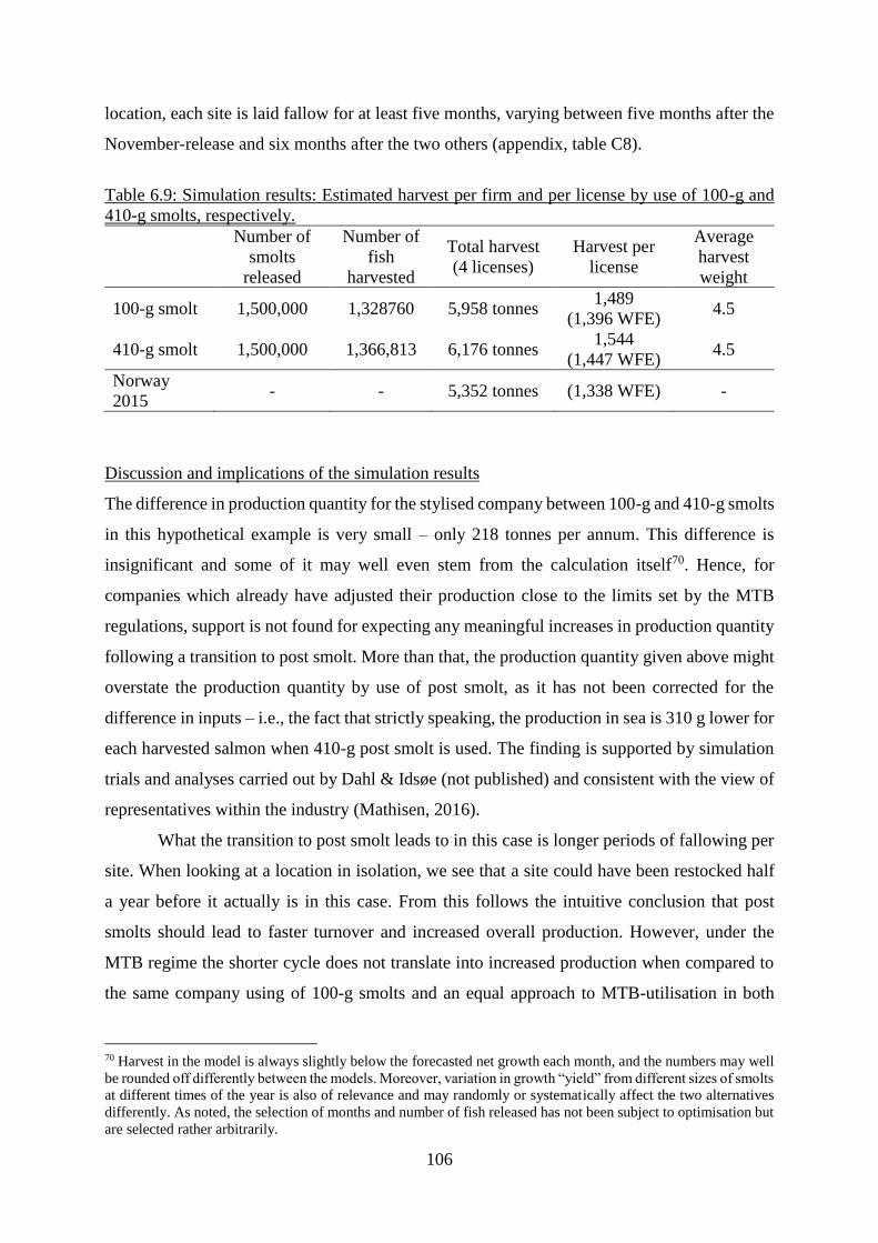
106

location, each site is laid fallow for at least five months, varying between five months after the

November-release and six months after the two others (appendix, table C8).

Table 6.9: Simulation results: Estimated harvest per firm and per license by use of 100-g and

410-g smolts, respectively.

Number of

smolts

released

Number of

fish

harvested

Total harvest

(4 licenses)

Harvest per

license

Average

harvest

weight

100-g smolt 1,500,000 1,328760 5,958 tonnes 1,489

(1,396 WFE) 4.5

410-g smolt 1,500,000 1,366,813 6,176 tonnes 1,544

(1,447 WFE) 4.5

Norway

2015 - - 5,352 tonnes (1,338 WFE) -

Discussion and implications of the simulation results

The difference in production quantity for the stylised company between 100-g and 410-g smolts

in this hypothetical example is very small – only 218 tonnes per annum. This difference is

insignificant and some of it may well even stem from the calculation itself70. Hence, for

companies which already have adjusted their production close to the limits set by the MTB

regulations, support is not found for expecting any meaningful increases in production quantity

following a transition to post smolt. More than that, the production quantity given above might

overstate the production quantity by use of post smolt, as it has not been corrected for the

difference in inputs – i.e., the fact that strictly speaking, the production in sea is 310 g lower for

each harvested salmon when 410-g post smolt is used. The finding is supported by simulation

trials and analyses carried out by Dahl & Idsøe (not published) and consistent with the view of

representatives within the industry (Mathisen, 2016).

What the transition to post smolt leads to in this case is longer periods of fallowing per

site. When looking at a location in isolation, we see that a site could have been restocked half

a year before it actually is in this case. From this follows the intuitive conclusion that post

smolts should lead to faster turnover and increased overall production. However, under the

MTB regime the shorter cycle does not translate into increased production when compared to

the same company using of 100-g smolts and an equal approach to MTB-utilisation in both

70 Harvest in the model is always slightly below the forecasted net growth each month, and the numbers may well

be rounded off differently between the models. Moreover, variation in growth “yield” from different sizes of smolts

at different times of the year is also of relevance and may randomly or systematically affect the two alternatives

differently. As noted, the selection of months and number of fish released has not been subject to optimisation but

are selected rather arbitrarily.

107

cases. Importantly, however, the analysis disregarded restrictions at the level of locations. With

the same number of locations and the same approach to production planning and harvest in

response to MTB-constraints in both cases, it was not seen how a transition to post smolt

automatically leads to increased harvest.

The assumption that the MTB at the location level is not a constraint may not always

hold true, particularly for smaller companies with more limited access to locations, fewer

permissions and geographical concentration. If, in contrast to our simulation, access to locations

or limitations at the level of location-MTB is inhibiting a company from utilising company-

level MTB – then it may be that post smolt is a way to address such constraints and thus increase

overall production. In general, it seems that the potential for such a production increase is

dependent on the specific company’s situation in the first place: In the event that companies

have suboptimal MTB-utilisation, then post smolt may offer increased flexibility so as to fulfil

unrealised potential.

Nevertheless, this is very much an area for further research. In the examples given, only

one example of a company in possession of a certain number of locations and permissions was

examined. For further studies, the relationship between the number of permissions and locations

could be varied. A relevant extension is also to examine various firm sizes and to look at the

effect on production from harvesting more and less frequently – although this is more of a

general question about production potential than a question related to different sizes of smolts.

It is clear that daily harvest gives room for an average biomass much closer to the MTB,

implying that the daily net growth would likely be both bigger and harvested more often71.

According to industry sources, the largest companies can harvest the net growth every day,

whereas this is not likely the case for the smallest firms. In terms of differences between small

and large firms in Norway, this is relevant.

It is also relevant to explore how the difference in growth relative to fish size affect the

possible harvest quantity with use of large and small smolts. In relation to fish size, growth

(production) as a percent of the biomass is decreasing with increasing fish size72. In turn, this

could favour a lower average fish weight to maximise the net growth that can be harvested per

period. In the examples given, it has been assumed that three batches of smolts of equal sizes

are released every year. The model could easily be extended by considering more batches than

71 This simulation has aimed to shed light on the similarities and difference between smolt sizes, and hence more

emphasis is put on equal conditions than the effect of various condition of the total harvest. 72 This statement is a bit problematic in light of current production challenges, where disease and health issues

mean that growth relative to fish weight is not only dependent on fish size, but also fish health, sea lice and lice

treatments and possibly therefore affected by the length of the production cycle itself.

108

three. Moreover, production optimisation may imply that batches should not be of equal size

and number. Finally, and possibly most importantly, simulations with variation of regulations

should be considered. In the examples above, there are MTB-regulations at the location and

the company level, but the latter is seen to “drive” the harvesting.

This contrasts to the situation and the regulatory framework on the Faroe Islands, where

the introduction of post smolts appears to have led to a considerable increase in production

(Østergård, 2016). From 2000-2005, Faroese salmon aquaculture was ravaged by Infectious

Salmon Anemia (ISA/ILA), leaving the industry in immense difficulties. The crisis led the

industry to implement what is probably the most stringent legislation among salmon

aquaculture producing countries (Kyst.no, 2017b). Since then, the Faroese industry has

transformed to become what may well be the most biologically and environmentally sustainable

salmon production regime (Østergård, 2016; Kyst.no, 2017b). As noted, the Faroese industry’s

rate of mortality is about half that of Norway’s (Hjeltnes et al. 2017).

In terms of production permissions, Faroese legislation imposes restrictions on fish

density measured as kg/m3, but no MTB. Under this regime, Hiddenfjord is one of the Faroese

salmon aquaculture firms that has experienced great success with transition to the use of post

smolt (Østergård, 2016). Although the primary benefit of post smolt is emphasised as risk

reduction in relation to disease, sea lice and accidents in sea, the company reports a major bonus

in terms of increased production and improved utilisation of production licenses. As an

example, they look at an 84-months’ period, i.e., seven years. By use of small smolts, as was

common earlier, a production period in sea would consist of 19 months of growth and two

months of fallowing – occupying a location for a total of 21 months. In seven years, the

company would be able to do four productions. By transition to post smolt, a production period

would be reduced to 12 months of growth followed by 2 months of fallowing – occupying the

location for a total of 14 months. In seven years, the company would be able to do a total of six

productions at the location – an increase of 2 productions in seven years, corresponding to a

50% increase from the previous four, following the introduction of larger smolts.

In this case, it is clear that the transition to post smolt has led to an increase in

production. The constraining factor when it comes to biomass under this regime is determined

by the maximum density, which is reached just before the point of harvest73, while importantly,

a site is limited to only one generation of fish. Hence, when the required (and desirable) period

73 Hence, the number of fish released is adjusted in order to have a generation of at a desirable harvest weight

when the biomass approaches maximum density (with due allowance for mortality).

109

of fallowing is completed, there is nothing inhibiting the firm from releasing a new generation74.

Under company-level MTB in contrast, a company is inhibited from releasing additional fish

because of its existing biomass in other locations75.

Still, it must be noted that differences between Norwegian and Faroese operating

conditions are not limited to the difference between Norway’s MTB and Faroese kg/m3.

Importantly, there are several other regulations on the Faroe Islands – and, crucially, the

industry structure is very different; probably with some fundamental impacts on how the

Faroese Aquaculture Act can be maintained. For the purpose of this review, one practice seems

particularly relevant when assessing the implications of the Norwegian MTB so it is reasonable

to mention this.

A unique and vital part of the aquaculture legislation of the Faroe Islands is the “all-in,

all-out strategy” (kyst.no, 2017b). Each location or production site is limited to only one

generation of salmon and between each Faroese generation, all equipment must be dismantled,

thoroughly cleaned and approved by the Food and Veterinary Agency (ibid.). Thereafter, the

site must lie fallow for a minimum of two months before a new generation can be released to

the fjord. But more than that, the Faroese producers coordinate fallowing and set a limited time

window for release of new generations so as to have all locations in a fjord fallow at the same

time (FFFA, n.d). Before the new legislation, continuous production in a fjord was the norm

(kyst.no, 2017b). That is, as harvestable fish were taken out at one location, smolts were released

at another. In terms of biosecurity and room for disease and parasite accumulation and

transmittal, the difference may well be profound.

Because of different industry structures, the feasibility and practical possibility of

maintaining such practices are profoundly different in Norway than the Faroes – regardless of

legislation. Nevertheless, it may be worthwhile to consider how the MTB-regime may actually

contribute to counteract attempts to coordinate fallowing and improve upon biosecurity in

Norway. In particular, smaller, geographically concentrated and less flexible producers may

suffer penalties in terms of license utilisation under efforts to coordinate fallowing in general

and/or within production zones (Salmon Group, n.d; Ilaks.no, 2016b). Again, a thorough

investigation into this issue extends way beyond the scope if this study, but there are clearly

74 There are, however, other conditions – some of which will be returned to below. 75 Alternatively, it could probably reduce its number of fish released at all locations – in exchange for an increased

turnover. While this alternative design would allow the producer to an increased turnover while remaining below

MTB, brief and not extensive simulations seem to suggest that neither this would imply any meaningful increase

to total harvest provided that the producer adapts its biomass to remain close to the MTB at either production

design.

110

incentives for companies to maintain as continuous a production as possible given the locations

and MTB in possession in Norway (Guttormsen et al. 2012). Whether or not this could conflict

with concerns over and efforts towards enhancing biosecurity should be of interest for future

research. It is also interesting how under various coordination efforts, differences in company

size and geographical production distribution may lead to varying degrees of “penalties” for

companies in terms of output reductions – depending on each company’s flexibility in MTB

utilisation and production adaptation. In the context of new regulations to be introduced with

increased regional interdependency among its possibly consequences, the question seems

highly relevant (The Norwegian Government, 2017; The Norwegian Ministry of Trade,

Industry and Fisheries, 2016; IMR, 2015; NRK, 2017).

To be appropriate, a brief comment should be given about the Faroese industry

structure. First of all, the country is a very small producer compared to Norway. After the crisis

in 2000-2005, the industry underwent a significant transformation and consolidation, where the

number of companies was substantially reduced and is now down to just three, from about 20

at the time of the crisis (kyst.no, 2017a, FFFA, n.d). Clearly, this has implications for the ability

and incentives to coordinate and cooperate. Locations have also been defined and separated

more carefully (FFFA, u.d.). If locations are to be operated independently, a distance of

minimum 5 km is required; if the distance is less, they must coordinate (ibid.). The country is

otherwise small and located in relative isolation with strong currents and efficient natural

ecosystem services. However, favorable natural conditions did not inhibit the industry from

collapsing prior to the introduction of its new regulation regime in the mid ‘00s.

6.4 Summary

This chapter has provided indications that under the assumptions in this study, sea based cost

of production looks likely to increase somewhat following the introduction of larger smolts.

Meanwhile, the possibility of countering this cost increase by increased revenues, production

quantity and MTB utilisation seems to be limited to those firms with a “suboptimal” utilisaton

of permissions in the first place. The extent to which Norwegian companies in general are able

to utilise their MTB optimally is not clear76. However, as chapter II illustrated, the ability to

produce more per permission has increased continuously over time, potentially suggesting that

further “underutilised” potential may still exist. Indeed, Dahl & Idsøe (2016) note that the

Norwegian industry has nearly doubled output over time in spite of only marginal increases to

the industry-wide total MTB. Looking at the relationship between production output and total

76 From official statistics, only the average output per license can be read.

111

MTB issued for the industry as a whole, this increased from 0.9 in 2005 upon the introduction

of the current regulations, to 1.7 in 2015 (Dahl & Idsøe, unpublished).

Although the average quantity sold per permission in Norway has increased over time

– also before the introduction of the current MTB in 2005, it is interesting to note that the

increased has occurred much in parallel with the increase in firm size and the average number

of licenses per company (see chapter II). However, even if production quantities per license

have increased while companies have become larger over time, explanations for this could also

include technological progress, learning and other effects.

Dahl & Idsøe also note that there are considerable variations in MTB utilisation at the

company level. In 2014, data on 95 Norwegian salmon aquaculture companies showed that the

average company extracted 1.8 tonnes per tonne MTB (ibid.). At the same time, 20 companies

exceeded 2 tonnes per tonne MTB – some approaching 2.5 tonnes of ouput per tonne MTB

(ibid.)77. Therefore, it seems clear that differences exist in firms’ ability to utilise licenses.

However, it is not known how large a share of the total Norwegian licensed MTB that belongs

to firms with relatively low and high MTB utilisation, respectively. A review of the MTB

regime in 2012 stated while “today’s production capacity is different from today’s production”,

the actual capacity “is not quite known” (Guttormsen et al. 2012). The same study gave a careful

estimate, stating that within the existing licensed MTB in 2012, production could probably be

increased a further 10% from the current production, which was then estimated to be around

1.2 million tonnes in 2012. While the study by Dahl & Idsøe noted that there are considerable

differences in MTB utilisation between companies, Guttormsen et al. (2012) noted that it also

differs substantially among regions78.

How different companies approach the MTB utilisation problem with and without post

smolt seems to be an interesting topic for further research. The way in which these strategies in

turn may influence and be influenced by needs for cooperation and efforts towards biosecurity

should also be of interest. One such question is whether company-MTB on the one hand – and

initiatives in the form coordination within zonal regions on the other hand – impose conflicting

restrictions and incentives upon some firms. In the worst case, this might involve unintended

penalties for biosecurity enhancement and rewards for maintaining a most possibly continuous

production. Given the nature, accumulation and dissemination of transmittable diseases and

parasites such as sea lice, the questions seem important.

77 It was also observed that some companies had considerable variations from year to year in the quantity they

were able to extract – without simultaneous changes to their available MTB. 78 Which may be natural as a consequence of differences in sea temperature and correspondingly in net growth.

112

Notwithstanding the likelihood of increased smolt cost, numerous companies are

incorporating post smolts as a main component of their strategy. This could indicate several

different things79. Possibly, many companies could for various reasons be in a position where

there is room to improve their MTB utilisation from the current situation. It could also be that

the actual cost of post smolt production is lower than our estimate. Alternatively, it could be

that the costs associated with sea lice and biological issues in our calculations are

underestimated – and that the savings associated with post smolt, shorter production cycles and

less mortality should be higher than outlined in our calculations. Similarly, the industry may

expect that sea based challenges will increase from here, so that the benefits will weigh up for

the cost in the future. Given the recent development in sea related challenges, companies may

see a post smolt strategy as a way to lower production risk and increase production control –

and that risk reduction may itself defend a cost premium. The latter points are far from irrelevant

– the Norwegian veterinary institute’s fish health report for 2016 reveal that increasing

resistance among sea lice to medical and chemical treatments has led to a major shift to

mechanical lice treatments (Hjeltnes et al. 2017). At the same time, in their survey, 93% of fish

health personnel reported increases in fish mortality and damages following this type of

treatment (which compares to 65% related to medical treatment options). Given the resistance

issue and related increase in mechanical treatments, the report notes that mortality associated

with lice treatments is poised to remain as large a challenge also in 2017 (ibid).

79 Of course, the estimated smolt cost and other assumptions underlying the analysis may be one potential reasons

as well.

113

VII LAND BASED SALMON - MARKETING OPPORTUNITIES

As outlined in chapter II, today’s salmon production is primarily concentrated in a handful of

countries where the natural conditions are suitable for farming of this species. These countries

are Norway, Chile, Scotland, Canada and the Faroe Islands. Typically, the domestic

consumption in these countries is relatively limited, with much of the production being traded

internationally (with the exception of Scotland’s production where a substantial share is

marketed in the domestic UK market). Export destinations for salmon are found across the

globe. Notable market destinations for salmon include the EU, the US, Japan and Russia. As a

rule of thumb, current salmon supply is transported over a long distance.

While land based facilities are being planned across a diversity of continents and regions

– including in major salmon producing countries such as Norway – it is commonly emphasised

that investment in land based salmon aquaculture has a central feature in allowing salmon

production to be located closer to the main markets (other potential advantages include control

over the internal aquaculture environment, waste and interactions with the environment; see

chapter II). A major advantage to the flexibility in location is the expected cost advantage from

saved transportation costs – especially to markets to which today’s salmon supply is transported

by costly air freight. As illustrated in table 7.1, the cost of air transportation per kg of salmon

may amount to as much as NOK 14/kg HOG (DNB, 2017), while other sources indicate NOK

8/kg in air freight from Oslo to the US.

Table 7.1 Total cost to US (or Asian) market for Norwegian sea based and US (or Asian) land

based salmon, respectively.

NOK/kg Sea based (Norway) Land based (market)

Farm gate cost of production 28.5 38.7

Harvesting 3 3

Total per kg (WFE) 31.5 41.7

Total per kg (HOG) 35.5 46.9 Air transport packaging 1 0

Inland transport 1 1

Air transport (US/Asia) 14 0

Total per kg (HOG) 51.5 47.9

Source: DNB Markets (2017) for costs after farm gate cost of production (as estimated in

chapter IV).

Another result of having more flexibility in locating production is the possibility of

targeting locations with the best operating conditions for the industry. One point in that respect

is the industrial policies in place in various countries. For instance, the EU operates support

programmes for fish processing and aquaculture which are not available in a traditional salmon

114

producing country such as Norway (Bjørndal & Ellingsen, 2016). Together with taxes and

import duties, such policies aim to strengthen the competitiveness of EU member countries and

improve the region’s self-sufficiency of fish. Moreover, many countries where land based

salmon farming may be established have lower labour costs than Norway.

Accordingly, a direct comparison of cost of production and delivery to market might be

more complicated than adjusting for transportation costs. At least in the short term, the

availability of a transportation and supply infrastructure and network can have implications for

both cost and efficiency of production in new locations. Even production plants located within

the national markets require domestic transportation. There is also an unknown magnitude of

economies of scale effects – in production, but possibly also in terms of industrial proximity

and clustering of support services and related industries, including processing, veterinary

services and the sharing of knowledge. Given regulations, scale effects, industrial policies and

potential benefits of industrial proximity, one can also envisage competitive advantages other

than the sole priority of locating land based facility as close as possible to major markets.

In addition comes differences in the availability, quality and cost of inputs such as water,

energy, land and competent labour. Differences in regulations and attitudes towards genetically

engineered food is also likely to become a more potent and relevant topic as more regions and

nations enter production. Genetically modified (GM) salmon is already underway in the US,

where AquaBounty Technologies, a Nasdaq-listed firm, is planning its first commercial scale

facility for growing eco-friendly “AquAdvantage salmon,” which should not require vaccines

or antibiotics (Intrafish, 2017). The company expects to harvest its first salmon in the third

quarter of 2019.

Atlantic Sapphire, a Norwegian, newly OTC-listed salmon farming company in the

process of constructing a land based plant in Florida, may provide some indications of the

expected economies of scale in land based farming. Atlantic Sapphire aims to reach a 2026-

production of over 90,000 tonnes and become the most competitive supplier of salmon to the

US by using scale to reduce operating costs to levels close to traditional salmon farming –

combined with minimal transport cost to the key US market (Undercurrentnews, 2017).

According to the company’s own fundraising presentation, it aims to bring its costs of supplying

salmon to US customers below those for Norway and Chile (ibid).

7.1 Ecological and organic production, product certification and marketing of salmon

As noted in chapter II, global megatrends in the food and consumer markets include increasing

awareness towards health and nutrition, sustainability and traceability in food production.

115

Consumers’ concerns about the environment, health, food safety and food origin may present

opportunities as well as challenges to aquaculture production, where pollution, pesticides and

the use of medication and antibiotics historically has been a challenge to the industry’s

reputation. As noted, new technologies and production models may represent ways of

addressing some of these concerns. Land based producers have frequently noted these trends,

seeing opportunities for product differentiation by emphasising a sustainable, fully traceable

and potentially domestically produced salmon.

Indeed, one of the central marketing claims from potential entrants to land based salmon

aquaculture is its environmental advantages and opportunities for producing organically80. The

principal claim of organic production is to offer a long-term perspective for sustainable

aquaculture at three levels: social, ecological and economical (Aquaculture Europe, 2013).

Organic aquaculture is regulated through the EU regulations on organic production and

labelling of organic products (EU Council Regulation 2092/91). The EU organic logo and

labelling rules are an important part of the organic production regulations (European

commission, n.d.).

Aquaculture Europe, a magazine published by the European Aquaculture Society,

provides production statistics for organic fish production in 2012 for the main European

producing countries (Aquaculture Europe, 2013). With more than 80 % of the whole European

organic production, salmon was the major certified species in Europe in 2013 (ibid). However,

as a share of the total European salmon production, only 1.4% was organic in 2012. The main

organic salmon producer was Ireland. It produced 9,600 tonnes – half of the European organic

salmon supply, accounting for 70% of the country’s total production. Most of it went to French

and German markets. While Norway accounted for more than 80% of the total European

production, less than 1% of production was labelled as organic (about 8,000 tonnes) – with all

organic production going mainly to the UK and Germany. During the five years prior to 2012,

the production of organic salmon had decreased as a function of higher costs in a difficult

market with cyclical prices. Furthermore, the use of medicines to control diseases and parasites

(especially sea lice), the effects of escapees and the increasing use of land-based vegetables in

80 In organic/ecological production, natural resources are to be managed so as to avoid harm to the environment.

Ecological aquaculture implies that operations are managed with care and concern for the environmental footprint

as well as the health and wellbeing of organisms. It entails farming of various species as well as harvesting,

transportation and sales of the products and may include a focus on local and renewable resources. The surrounding

environment should be affected as little as possible by the operations, including any transfer of disease, parasites

and medicines to the wild. Feeding is managed so as to contribute to a natural feed intake with minimal waste.

Feed ingredients (oil and meal) should stem from organic agriculture or from the fish waste generated by

sustainable fisheries, with the feed often involving a large share of marine ingredients. Additives are not allowed

in organic feed.

116

salmon feeds had been challenges to organic certification. Hence, only two farms were certified

organic in Norway in 2009 (ibid). In the UK, 14 farms produced 6,122 tonnes of organic product

in 2010. However, in 2011, only about 2,900 tonnes was produced.

In its 2012 Annual Report, the Federation of European Aquaculture Producers (FEAP),

outlined the main challenges in organic production – including feed specifications, husbandry

measures, limited stocking densities and higher costs (Aquaculture Europe, 2013). National or

local legislation is not always adapted and often prevents producers from starting organic

production (ibid). Moreover, the term ‘organic’ is also interpreted in a multitude of ways and

the number of certified labels does not help consumers to see more clearly (ibid).

There are currently no special organic certificates available for land based salmon. The

existing European standards for organic salmon require a maximum of 10 kg of fish per m3 to

avoid stress or skin damage and to allow the fish to shoal (Debio.no, n.d.). In Norway, none of

the planned facilities assume a fish density below 40 kg per m3, and land based operations

would struggle to reach profitability at such low densities.

As of today, organic salmon seems to be a relatively limited market niche in terms of

overall quantities, although an updated set of data has not been obtained – either for production

or prices. Aquaculture Europe noted in 2013 that “if organic production becomes more than a

niche market, it loses its inherent market premium. As other standards and ecolabels are used

to demonstrate aquaculture credentials, the option to produce to organic standards should

logically be based on small volumes to satisfy relatively small demand” (Aquaculture Europe,

2013).

In terms of ecolabels and other standards for sea farmed salmon, other, less

comprehensive certificates than the organic standards are already being more widely applied.

The Aquaculture Stewardship Council (ASC) is an independent, international non-profit

organisation that manages the world’s leading certification and labelling programme for

responsible aquaculture (asc-aqua.org, n.d.). The ASC salmon standard has been in operation

since 2012 and aims to address the key negative environmental and social impacts of salmon

farming associated with: sourcing of feed ingredients, disease transmission between farms and

into wild salmon populations, controlling escapes into the wild, use of therapeutics and anti-

biotics, site impacts, the presence of GMO products in feed and labour issues on farms (asc-

aqua.org, n.d.).

All farms certified to the ASC Salmon Standard must meet a total of 154 performance

criteria and 521 compliance criteria, thereby showing they deliver real environmental and social

benefits (The Fish Site, 2017). Recently, in June 2017, ASC certified farmed salmon also

117

became officially endorsed by the Monterey Bay Aquarium’s Seafood Watch standards as a

‘Good Alternative’ and a recommended, sustainable form of seafood (ibid.). Their ‘Best

Choice’, however, is Atlantic salmon farmed worldwide in closed tanks (labeled as "land-

based" or "tank-based" salmon), following the arguments that closed tanks often have less

effluent, disease, escapes and habitat impacts than other aquaculture systems (Seafood Watch,

u.d.). Currently, only 0.1% of farmed Atlantic salmon is produced in closed tanks (ibid.).

At the end of 2015, the number of ASC certified aquaculture farms exceeded 200

globally (Wwf, u.d.). Salmon was the largest product group, with 84 out of the total number of

farms – most of which were located in Norway (ibid.). At present, nearly a quarter of all famed

salmon produced globally is ASC certified, and members of the Global Salmon Initiative (GSI)

are the main sources of ASC-certified farmed salmon. The GSI is a collective of the leading

global salmon farming companies that have made it their target to be 100% ASC certified by

2020 (The Fish Site, 2017). Polish aquaculture producer Jurassic Salmon became the first land

based salmon farm to achieve ASC certification in 2016. It is also the world’s first fully organic

Atlantic salmon farm, using thermal ground water from 150 million years ago (Fish Update,

2017).

7.2 Could there be a price premium for land raised salmon?

Expectations and speculations about the possibility of a price premium for land raised salmon

tend to be grounded in beliefs about possibilities of organic production practices and

certification schemes, as organic products tend to fetch higher prices in the market. Some

attributes that the land based aquaculture producers might seek to emphasise include:

- Management of the aquaculture environment to best possibly meet the needs of the fish

- Waste control and possible reuse/recycling of the waste

- Disease and parasite control (particularly with respect to interactions/transfer to the

wild)

- Possibly reduced need for chemicals and treatments – at least reduced or more

controllable impact of such use on the surrounding ecosystems

- Fish welfare and associated product quality

- A safe and controllable working environment

- Origin/locally sourced food

For land based salmon to realise premium prices in the market, the relevant product

attributes would need to be accepted by consumers and associated with land based production

in general, as superior to sea based alternatives. Trusted certifications schemes might be one

118

way to build an organic image, while branding by single producers likely requires substantial

scale to achieve the same. It is anyway hard to expect the outcomes in advance, and the question

of both price premium and sustainability of production might depend on individual firms’

strategies and level of success.

As previously referred, a study by Liu et al (2016) compares the carbon footprint of

salmon produced in traditional open net pen production system in Norway and a model

freshwater RAS facility in the US. According to their findings, the carbon footprint of land-

based salmon produced in the US and delivered to the US market is less than half of that of

salmon produced in traditional open net pens (ONP) in Norway and delivered to the US by air

freight81. When comparing the carbon footprint from production only, the RAS-produced

salmon (assuming the average US electricity mix) has a carbon footprint that is double that of

the ONP-produced salmon. Assuming use of energy from water only, the carbon footprint is

fairly close for the two alternatives, but still slightly higher for RAS. Consequently, conclusions

and promotions about climate friendly production modes will likely need to be considered more

carefully than just based on the production technology itself.

The spread in operational and biological success among all land based operations might

also affect the image of the producer group as a whole. Just like there is variation in production

practices among sea based producers and producer countries, there could also be a wide range

in the level of fish welfare, medical use, waste management and product quality among land

based salmon farms globally. In that sense, certification schemes might be more of a

differentiator between good and bad producers than between good and bad technologies. Still,

differences between technologies with respect to the availability and ease of achieving and

proving the required performance to be certified could come to exist. As certification schemes

of varius sorts become more mainstream and widespread, expectations are also evolving and

one might ask whether various certifications themselves will enable price premiums in the long

run – or if they increasingly will be expected or even required to get access and contracts in the

distribution chain.

Nevertheless, local or domestic production might give land based farmers an edge in

their marketing efforts. This could both take the form of consumers’ preference for local

products and their own country of origin as well as the possible marketing intelligence that

81 The results of the carbon footprint analysis confirmed that production of feed is the dominating climate aspect

for both production methods, but also showed that energy source and transport methods are important. It was

shown that fresh salmon produced in RAS systems close to a US market that use an average US electricity mix

(coal 50%, water energy 50 %) have a much lower carbon footprint than fresh salmon produced in Norway in ONP

systems shipped to the same market by airfreight, 7.41 versus 15.22 kg CO2eq/kg salmon HOG, respectively.

119

results from proximity to consumers; sensitivity to and understanding of their product

preferences and habits. In general, product quality, consistency and reliable distribution are

important for market access and price. While it is possible to assume that land based facilities

could get their fish to the local markets within a somewhat shorter time (at least to some market

places), questions such as the required scale of production and marketing make it difficult to

assume any distinctions between land and sea based production with respect to distribution.

The discussion so far about the price of land based salmon has centred on the potential

benefits of land based production. At the same time, less is said about potential benefits of sea

based production. Some counter arguments to expecting higher prices and a better image for

land based production could include a lower energy and oxygen consumption in sea, water

conservation, low fish density and generous space and the potential exclusiveness of fish that

are «raised in the wild». In contrast, land based salmon are in fact raised in factories at much

lower densities – which in other cases, such as in chicken farming, has rather less of a positive

image. Some possible challenges to product quality in land based salmon farming have already

been experienced by existing producers. These include skin damage resulting from high

densities, off-taste resulting from the water culture and early maturation. While companies

seem to report considerable improvement in managing, understanding and avoiding these

issues, much remains to be learnt and understood about the optimal conditions for fish in land

based systems.

When it comes to summarising expectations about the price of land based salmon, it

seems likely that the range of operating practices, fish welfare, biological and medical success

in farms around the world – together with marketing, certification schemes and quality control

– all will be part of determining the outcome in the longer term. While certified fish might

contribute to price premiums over non-certified fish, the discussion has indicated that it might

be optimistic to assume a price premium resulting from the production technology itself.

While this chapter has considered land based salmon compared to traditional sea based

salmon, another point about salmon price is the possible effect from the introduction of land

based technology on industry dynamics and structure as well as the global price of salmon. This

will be left for a brief discussion in the next chapter.

120

VIII SUMMARY AND DISCUSSION

To summarise the findings and results from the research, this chapter will discuss each of the

main analyses separately before closing with a recommendation of areas for further research.

First, land based farming of salmon is discussed in chapter 7.1, with emphasis on

competitiveness and comparison with conventional production. Second, the analysis of land

based production of post smolt is discussed in chapter 7.2. The findings about post smolt grow-

out in sea are discussed in chapter 7.3, both in terms of cost of production and issues related to

production planning.

8.1 Land based farming of salmon

This study has indicated that with today’s knowledge and under the assumptions presented,

land based salmon aquaculture technology might offer an interesting and economically viable

way of producing salmon. Yet importantly, the cost of production analysis indicated that to be

profitable, land based producers might still need to fetch a higher price than sea based farmers

need – at least in a Norwegian context82. This means that a land based investor in this context

takes on considerable market risk – in addition to the biological and technological risk. Should

the balance between supply and demand change in the future, that is a risk for producers with

a higher cost of production. Nevertheless, the technology is still in its earliest phase and entrants

may be expecting that as technology progresses and biology is increasingly well understood,

production may be expanded, economies of scale and learning effects realised and cost of

production come down.

The comparison with other studies showed that the estimated cost of production in this

study is relatively high – although the estimate made by Liu et al. (2016) based on a US context

is not very far below. Still, as underlined, with respect to the existing literature the context as

well as the assumed cost structures are different from study to study. And equally important,

we are talking about a new technology so that empirical data on cost of production of this scale

are non-existent. For this reason, it is acknowledged that adopting a stochastic methodology

such as King et al. (2016) could have contributed an added value to the deterministic approach

used in this study. Their study addresses the implications of economic risk on technology

selection by incorporating stochastic variance in a comparative analysis of salmon grow-out

production models. An important argument for doing this is to enable decision makers to

develop an awareness of economic risk by visualising differences in variability of expected

results. Without accounting for variance in investment appraisals managers might not make the

82 The analysis looks at farm gate cost of production before harvest, processing, transport and sales related costs.

121

most appropriate decisions (King et al. 2016). The current analysis accounts for risk and

uncertainty by undertaking sensitivity analyses for specific components to reveal specific risks

and areas of importance. Although that is useful and contributes important managerial insights,

it does not reveal the variability profile for a project as a whole (which is of interest in a

decision-making situation). This could be an area for further research.

In terms of comparing land based cost of production with the alternative production

modes, the current study has its limitations with respect to the sources of data used. The

approach to data collection and analysis is very different between the land based and the sea

based production parts. The official statistics used to analyse sea based operations are from two

years back in time (2015), and with a correction for interest on license values as shown in

chapter VI. Land based data are collected in 2017, based on expectations. Part of the

discrepancy could be addressed by accounting for inflation. However, another issue would

remain, which is the possible increase in lice related costs since 2015. Given the recent

development in lice treatments and treatment resistance problems, it is possible that the 2015

data underestimate the lice related costs of today.

Table 8.1 summarises the estimated farm-gate cost of production per kg (WFE) by use

of full land based grow-out, traditional production (2015) and 410-g smolts. The last row

remains empty as a reminder of the uncertainty related to current lice related costs in sea based

production. If the cost is inflated to 2017-prices, the cost of production per kg for the two latter

scenarios becomes NOK 29.74 and NOK 31.13, respectively83.

Table 8.1. Cost of production per kg (WFE). Land based full cycle production and sea based

grow out of 100-g smolts and 410-g smolts, respectively.

Land based

NOK/kg

Traditional

farming (2015),

100-g smoltsa)

410-g post

smoltb)

Feed 16,1 13,18 13,18

Roe/smolt 0,3 2,72 7,19

Labour 2,3 2,07 1,68

Other variable costs 12,5 6,44 4,44

Sum variable costs 31,2 24,41 26,49

Interest and depreciation

on investments 6,6

3,97 3,22

Other fixed costs 0,16 0,16

Sum fixed costs 7,5 4,13 3,39

Total production cost 38,7 28,54 29,88

83 The figure is for 2015 and has been adjusted to 2017 level to account for price increases (CPI 2015 = 100,

January 2017 = 104.2).

122

Increase in cost of sea lice since

2015 - ? ?

a) With own estimate added for interest on license value.

b) This cost is based on increases in production quantity and turnover as estimated in

chapter 6.1: Assuming an increase in production equivalent to the increase in turnover

following a transition to 410-g smolt (corrected for smolt weight) – leading to lower

cost per kg from labour, interest and depreciation as well as a reduction of NOK 2/kg in

lice related costs. If we instead assume that the cost of production per kg stays the same

as in traditional farming (2015) and add the increase in smolt cost per kg (7.19-2.72)

while subtracting NOK 2.0 in anticipation of less lice treatments, then the cost of

production becomes 31.01/kg. The difference is relatively small because as noted in

chapter VI, lice related costs are assumed to constitute the most important potential for

cost savings by use of large smolt.

As the table shows, farm-gate cost of production is expected to be higher in land based

than in sea based grow-out, while production using large smolt is a bit costlier than 100-g smolt.

The engineering costs used to estimate land based full-cycle production and cost of production

per 410-g smolt might not be directly comparable with the average production costs reflected

in official statistics. Moreover, the pricing or transfer price of smolts represent another problem

for the estimated cost of production. For an integrated firm, the smolt price might have been set

differently than that in our study. As recalled from chapter V, the smolt price paid by sea based

grow-out farms includes a margin – also reflected in the positive NPV which was estimated for

investment in post smolt production. Again, it can be emphasised that the interest in salmon

producing firms is likely often neither the smolt price, cost of production or NPV from post

smolt production in isolation. Instead, the motivation relates to its impact on overall cost of

production and production risk for the firm as a whole.

For this reason, a complete analysis of an integrated firm with both smolt and grow-out

production is likely to provide the best picture of the attractiveness of investment in post smolt,

looking at both overall cost of production and NPV over a certain horizon. Such analysis was

not undertaken in this study, but a brief discussion of the separate findings is given below.

However, we shall first revert to an overall discussion of the price and market issues briefly

mentioned in chapter IV about land based competitiveness and relative attractiveness as an

investment opportunity.

It was noted in chapter IV that the price assumptions underlying the investment analysis

are formed in the context of constrained supply, good market demand conditions, a favourable

currency situation (in Norway) and cost related challenges in many traditional salmon

producing countries. Meanwhile, the NPV analysis suggests that there is potential for land

based salmon aquaculture to be a profitable investment opportunity also in Norway – but the

123

result is highly dependent on price. Given that market analysis and price forecasting is not done

in this study, the theoretical foundation for choosing a certain price and price development over

the projected horison is a weakness of the analysis. As noted, the price assumed was based on

the average forward contract price for the limited period for which it is available – and taken to

remain the same in real terms over the projected period in lack of a better estimate84. To consider

how and why this might be a weakness, it is worthwhile to look especially at the historical price,

as well as to the current price and the potential future price drivers.

Historical price

Historical real prices have, since economies of scale and learning effects were increasingly

exhausted after the 1990s, fluctuated but remained high relative to real cost of production in

real Norwegian kroner – in spite of increased global supply (figure 2.1). This is thanks to high

and steadily increasing demand – and, given that abnormal profits apparently have been

sustained for some time for the industry, it is likely also in part a result of high barriers to enter

the industry (in the form of both regulations and natural conditions).

Current price

Compared to historical prices, the real salmon price level – particularly in NOK – over the last

few years (2015-2017) is very high. For the Norwegian industry, where most of the quantity is

exported, the exchange rate situation must be considered in order to evaluate the price faced by

buyers in the market. In 2015, Norway experienced record high seafood export values, in

particular for salmon (and cod). However, while exports increased by 8 percent in terms of the

Norwegian krone, in US dollar terms they declined by 16 percent. The fact that the Norwegian

currency has been relatively weak in recent years (following the oil crisis starting in 2014) has

helped Norwegian salmon exports to stay competitive in spite of rising cost of production.

Hence, should the currency strengthen, this may very well be expected to put pressure on prices

in real Norwegian terms – which might be painful if the current cost trend is upheld85.

Future expectations – price, demand and supply

In the future, prices as well as exchange rates between countries may change. The latter factor

is nearly impossible to foresee and to account for. Otherwise, as far as prices are concerned,

both supply and demand are central. It is not possible to predict future development in either of

84 That was a bit less than three years forward in March 2017, to the end of December 2019. 85 Although possibly costs such as imported feed may weigh up. However, this need not necessarily work as a

currency hedge either, as relative developments in the feed producing currency may not coincide with the

development in salmon export destination countries.

124

the two within the scope of this analysis. Nevertheless, in analysing the feasibility of a

technology that has the inherent feature of bypassing current entry barriers to salmon

aquaculture, it would be conspicuous not to mention the potential feedback effect on prices in

the event that the technology succeeds. It would take quite a few land based salmon farms to

contribute a meaningful contribution to the global salmon supply – enough to affect the global

salmon price. On the other hand, as long as the outlook for increases in sea based production is

limited by disease problems and/or regulations, the expected NPV in a land based project may,

even with room for some biological challenges, look promising enough for many to take the

risk. In terms of new entrants, many seem determined to start out gradually, building out

facilities in smaller modules initially, before planning to expand production as biology,

technology and concepts eventually prove their success. One such example is Atlantic Sapphire,

which plans to build the first part of their US salmon aquaculture facility as a module with

8,000-tonnes production capacity, before expanding over time to 90,000 tonnes in a

development process consisting of three steps (ilaks 2017b).86

Moreover, factors that have been disregarded in this study may contribute to lowering

the bar: investment grants and subsidies, tax conditions; locational advantages in many forms;

advantages in logistics and transport cost; differentiation, marketing and consumers’ product

perceptions and preferences in terms of local produce, environmental impacts, concerns over

diseases and chemicals, etc., as well as potentially the regulatory environments87. Looking for

instance at the Atlantic Sapphire example above, important factors include transportation cost

advantage over exports from Norway (NOK 8-18/kg according to various sources, such as DNB

2017 and industry representatives). In addition, the company focuses on “made in USA” in their

marketing (ilaks 2017b). Looking at table 7.1, this transport cost advantage is sufficient to

weigh up for the difference in estimated farm-gate cost of production in land based and sea

based production in Norway.

With today’s price assumptions, knowledge and available technology, there are

incentives to invest in land based production for those who believe in their ability to manage

fish biology and to acquire the necessary competence to operate a fish farm. Should the first-

86 In comparison, the total import of salmon to the US was 133,175 tonnes in 2016, implying that the company is

aiming to supply 67.6% of the current import quantity (National Marine Fisheries Service, 2017). In terms of

strategy, this is an interesting signal or statement, potentially indicating both considerable scale advantages in

various forms (which could range from production, marketing, logistics as well as even risk) while it also reminds

a bit of a “preemptive” commitment signal. 87 Some of these factors, such as logistics, transport cost and taxes may also alter the relative cost of production

between the production modes. As Liu et al. (2016) showed, location of production closer to major markets may

also turn out to reduce the environmental footprint – at least to those markets where the current means of transport

is by air freight.

125

movers succeed, most have ambitions to expand production as soon as sensible to take

advantage of economies of scale (see table 4.1). On the cost side, new differentiators may

emerge based on locational advantages in many forms, as mentioned above.

Meanwhile, traditional sea based farms are striving to improve upon their operations

and take control over biology and related costs and build a foundation for sustainable

expansion88. Given the salmon price and the typical cost of production today, both modes of

production constitute attractive investments. In other words, under current limitations to global

supply, prices are sufficiently high to accommodate also producers with relatively high cost of

production. Indeed, investments are flowing into research, development and technological

solutions related both to traditional and alternative production models – in traditional as well as

some untraditional producing countries. Both the sources of future salmon supply and the price

consumers will be paying for it looks likely to depend in part on the alternative production

models’ absolute and relative ability to provide a healthy environment the salmon, where it can

be grown sustainably.

It is not easy to guess how the balance between supply and demand might change in the

future – or for that matter how soon any potential changes could be seen89. In theory, the

incentives to invest in land based aquaculture (in Norway) remains until price expectations

approach cost of production, which is adjusted for cost of capital. At this point, competitive sea

based producers (in Norway) would still have incentives to increase their production – if

regulations and biological conditions allow so. For this reason, in the event that land based

aquaculture succeeds on a large scale, it seems reasonable that a NPV analysis would need to

incorporate a declining price trajectory over the years, in line with expansion of global

production. Should sea based production also improve on biological issues and costs, prices

might be even more competitive in the future. It follows from this that the NPV-analysis for a

20-year period of an investment like this is highly uncertain.

Should the salmon price come down, this would also affect the value of existing

production permissions. That would be critical for any producer who had invested in a

production permission at the current value. This is important in terms of investment risk. While

production permissions probably have no alternative use, it is not easy to say anything about

the potential alternative use of a land based facility – a stranded asset or for instance of use in

88 History has previously shown that health related challenges may lead to needed actions and reforms, see for

instance chapter 6.3 for one example. 89 Of course, many considerations are relevant in that respect, including the relative prices of other products,

technological development and regulations, general economic developments and probably more.

126

production of other high value species. Aquaculture production in RAS systems is still in its

rather early development, so it is in many ways challenging to assess the riskiness of the

investment.

8.2 Post smolt production on land

The analysis of land based smolt production indicated that investments in production of post

smolt may be a profitable investment and that economies of scale might exist. Although there

are few references for comparison, the available estimates from other published sources showed

similarities in their findings of cost of production – but a question remains when it comes to the

shape of the cost curve as the smolts are grown larger in land based facilities. Cost of production

per kg is decreasing with increasing fish size, but it remains uncertain how and by how much.

Uncertainty in post smolt production is associated with variations in the technology and

level of investment as well as the related cost of production – labour demand, level of

automation, water sources (fresh or sea water), energy for pumping and heating (if the water is

to be heated), other cost of production, etc. In addition to differences in new-built facilities, the

solutions which can be found in the industry may vary even more90. With the data collected for

this study, it is therefore not reasonable to indicate or believe anything about the

representativeness of assumptions and results. Possibly, research at the intersection between

biology, technology and economy would be the most rewarding. For this reason, the discussion

of results and findings is drawn towards other areas such as technology and biology – where

many areas for further research can be found, but which are beyond the remit of this study.

Nonetheless, a central point with respect to the analyses of investment in production of post

smolt is that the investments are often done by integrated firms, whose interests are centred on

the overall company performance, cost of production and associated production risks. During

the land based phase, the risks may presumably be shifted to some extent from factors outside

of the farmers control – to more internal, manageable and controllable production risks. Control

of central growth parameters such as temperature in land based facilities may reduce the overall

production time and raise more robust fish for release to sea. Yet perhaps most importantly, it

reduces the grow-out period in sea substantially, thereby addressing problems related to sea lice

accumulation and exposure to transmittable diseases. For this reason, economic analysis of post

smolt is most valuable when analysed together with full grow-out operations.

90 Because of building standards and requirements to inhibit escapees, it seems that standards are generally high

in newly built facilities.

127

8.3 Post smolt grow-out in sea

The analysis of post smolt grow-out in sea provided indications that under the assumptions in

this study, sea based cost of production looks likely to increase somewhat following the

introduction of larger smolts. Chapters 6.1 and 6.2 anticipated how the cost of production in

sea based grow-out could be affected upon a transition to use of post smolts. It was examined

whether and how the increase in smolt cost (price) could be countered by potential rewards

from increased production turnover. It was argued that if new generations of fish can be released

and harvested continuously, there might exist possible savings in “capacity costs” (i.e., fixed

and perhaps some indirect costs). The reason is that those costs could then be distributed over

a greater production and hence reduce the cost of production per kg.

Chapter 6.3 examined further the possibility for such production increases by simulating

a production plan using 100-g and 410-g smolts, respectively. The objective was to examine

the potential increase in MTB-utilisation following a change to post smolt. A central assumption

in the simulation was that the company’s production capacity was determined by its number of

production licenses – i.e., its company-level MTB. The simulation illustrated the importance of

having as much fish as possible in sea at all times in order to maintain a continuous harvest as

high as possible. The findings showed that when the company is equally able to keep its biomass

at about the company-level MTB at all times in both smolt scenarios, support for expecting

meaningful increases in harvest quantity is not found. Thus, the possibility of achieving

increased revenues, production quantity and MTB utilisation by transition to post smolt is

dependent on a firm’s ability to maintain a company-level biomass about equal to the MTB in

sea at all times in the first place. Hence, a transition to post smolt does not automatically

translate into increased production when company-level MTB is assumed to be the only

constraining factor.

This finding might be a bit surprising, considering the expectations reported by several

companies and reports (Holm et. al, 2015; Kyst.no, 2017; Ilaks.no, 2015; Nofima, n.d.;

Rådgivende biologer, 2016). Two main explanations seem reasonable. First and foremost, the

assumptions in the simulation do in all likelyhood not hold true for all firms in the industry:

MTB at the level of the company is not the single determinant of production capacity. That is,

other constraining factors contribute to determine how much a company can produce given their

licenses. Although the other relevant constraining factors and how they impact individual firms

are not explained by this study, it seems likely that the number of locations and location-level

MTB constitute a central part of the explanation. The geographical production regions to which

a company’s locations belong add another dimension to the problem when regulations such as

128

coordinated fallowing or regional MTB apply. Modelling these issues is much more

complicated, because the number of locations, their respective location-level MTBs (and

relevant geographical region if associated regulations apply) and the number of permissions

associated with the locations vary individually between companies. For this reason, the effect

of post smolt on production quantity and cost of production per kg is also likely to vary

somewhat between companies. Those companies currently facing the most constraints to MTB

utilisation might see relatively more benefits from a transition than the companies at the top of

the range. For the former companies, both production increases and savings in capacity cost per

kg of production91 might potentially be achievable by use of larger smolts.

Another relevant and possible explanation for companies’ positive expectations and

investments in post smolt despite our simulated and cost related findings is the previously

discussed benefits related to fish health and sea based production risks. Comments from

industry representatives indicate that even the largest firms anticipate higher harvest from their

standing biomass with use of large smolts (200-300 g) as a consequence of larger daily net

growth and fewer lice treatments92.

As noted, the simulation carried out in this study was limited to a complete shift from 100-

g smolts to 410-g smolts – all else equal and with an equal approach to “full” MTB utilisation

(given a monthly harvest interval). Some companies that expect their MTB utilisation to

increase by use of post smolt may also be aiming to exploit the flexibility it offers in different

ways – to specifically address their relevant constraints to maintaining a continuous production

and a standing biomass close to the MTB. One example of this could be the use of large smolts

together with small smolts at a location in order to utilise location-level MTB (kyst.no, 2017d).

Large smolts may then be ready for harvest at a time when the company traditionally would not

have fish ready for harvest, and thus help to maintain a more continuous production93. While

that may allow a company to address MTB-concerns, other benefits of post smolt such as more

frequent fallowing do not seem to be realised when normal and large smolts are combined in

one location – potentially also conflicting with other biosecurity concerns, although this is a bit

of speculation. Anyhow, the ways in which MTB at various levels of regulation distort or affect

production patterns and firm behaviour seem to represent under-researched areas.

91 Such savings would depend both on the magnitude of the production increase and the amount of costs that are

fixed in for the relevant production range (i.e., not increased following the production change). 92 In our simulations, perhaps in contrast, daily/periodical net growth on the standing biomass is likely to be highest

with lower average fish weight because of decreasing relative growth with increasing fish weight. The effect of

sea lice on growth and mortality is not incorporated into our simulation. 93 See kyst.no, 2017d for an example.

129

8.4 Areas for further research

In terms of future research, topics of interest with respect to land based aquaculture of salmon

include a wide range of issues such as stochastic risk analysis of production and production

economy as noted above, the management of fish health, biological needs and water quality in

land based aquaculture systems, technological solutions, market and marketing opportunities

and environmental impacts. In terms of marketing, outcomes likely depend both on consumer

trends and concerns as well as the extent to which land based production proves able to control

the aquaculture environment and provide a chemical and disease free, sustainable/local/healthy

product with a limited footprint – while convincing consumers that they do so.

Many of the relevant research questions may well rely on conducting actual grow-out

trials and building experience with the opportunities and challenges of producing salmon using

this technology. Focus points noted by the industry include challenges such as early maturation

of fish, smoltification and choice of water sources and water quality parameters, light regime,

solutions for biosecurity and bacterial culture – for instance how many RAS units to have in a

facility and the trade-offs between biosecurity and cost of equipment and production, solutions

for fish handling, fish densities and water quality, feed quality and feed distribution system

(feed dust and particles in the water, etc.), off-flavour – purging procedure and duration, and

questions such as the design and size features appropriate for fish tanks (Olsen, 2017).

A number of areas for future research also relate to the increasing variety of smolt size.

Many questions relate to the interactions between technology and biology. It might be

considered whether such a discussion should be included in the summary of an economic

research – but associated with most of the questions are at least often economic tradeoffs. For

instance, a central question related to the level of investments is the chosen level of salinity –

fresh water, brackish water or salt water (industry source, personal communication). This in

turn has implications for the level of technological equipment and for fish biology94. This is just

one example. As discussed briefly under land based grow-out, many other questions are

94 With respect to biology, the smoltification process of salmon – where the fish naturally adapt from a fresh water

environment to a salt water environment – relies very much on salinity and has important implications for the

general development of the fish (ibid). When the fish are held on land rather than released to sea following the

smoltification process, this involves new questions in relation to optimal water conditions, timing and

smoltification. For now, industry practice seems to include both fresh water production and mixing of water

sources, allowing imitation of the smolts’ natural adaptation process – with smoltification and increasing salinity

starting already from when the salmon is 40-45 g (industry source). The former option (fresh water) allows

investments to be kept at a lower level, as technology and equipment for fresh water are less demanding. However,

in terms of biology this may involve delayed smoltification or de-smoltification, with potential/unknown impacts

on fish health, growth and development. The latter option, with increasing salinity and imitation of the natural

smoltification process, may require larger investments in order to step up the level and quality of equipment (such

as pumps, etc). On the other hand, the fish tend to go through a rapid growth phase following the smoltification

process, which should be realised and maintained under this approach (ibid).

130

relevant also here, including optimal fish densities, tank layout and water turbidity, water

chemistry, fish handling, etc. Vaccination strategy is also of relevance in both cases; normally

fish are vaccinated before saltwater adaptation due to exposure to transmittable diseases, etc.

from uncontrolled and unsterilised water. Gains from vaccination in terms of fish health and

disease outbreaks are substantial – but it has also been indicated that vaccination has by effects,

particularly when the fish are small. In the production of larger smolt on land, more flexibility

may be realised in the selection of an optimal vaccination time95.

The market for smolts could also be an interesting topic – including prices, transfer

prices, vaccination strategies and more. If most companies already have integrated smolt

supply, analyses with the perspective of integrated firms might be most relevant. As

emphasised, motivation for investment in post smolt extends beyond the outcomes from smolt

production itself – and to its role and impact on the overall company performance. Looking at

the sea based production phase, a question of great interest from both a biological and economic

point of view is the optimal point in time (and fish size) for release to sea. This depends both

on the cost of production on land versus sea, as well as relevant “bottlenecks”, such as sea based

production permissions and MTB at various levels.

How companies approach the MTB utilisation problem with and without post smolt

seems to be another interesting topic for further research, as discussed at length in chapter VI.

The current study analysed the effects of a transition from 100-g smolt to 410-g smolt,

attempting to reveal how production quantity would be affected by such a transition. However,

the analysis concentrated on company-level MTB, assuming that this limit would determine

harvest, and that location-MTB was sufficient enough not to become binding. An interesting

extension could be to look at constraints at both levels. This could be done by simulations as

well as by examining how companies actually adapt their production plans from their former

ones when introducing larger smolts. Questions include what their current constraints to MTB

utilisation are and how they use post smolt to address such constraints. That way, it could also

be shed light on how different production strategies vary in terms of sea based production risk

and approach to environmental and other concerns.

Whether or not the importance of having approximately the maximum permitted

biomass in sea at all times could conflict with concerns over and efforts towards enhancing

95 For more rigorous analyses of the biology of smolt production, it is referred to (for instance) Nofima. Biological

details and literature has not been studied in depth for the purpose of this study, so the questions and information

presented in this section are based on personal communication with the industry, observation of topics discussed

at conferences and variations in solutions and technologies observed under collection of information and data.

131

biosecurity should be of interest for future research. Likewise, the ways in which MTB-

utilisation strategies may influence and be influenced by concerns over biosecurity should be

of interest. One such question is whether company-MTB on the one hand – and initiatives in

the form coordination within zonal regions on the other hand – impose conflicting restrictions

and incentives. In the worst case, this might involve unintended penalties for biosecurity

enhancement and rewards for maintaining a most possibly continuous production if or when

the two objectives conflict. Given the nature, accumulation and dissemination of transmittable

diseases and parasites such as sea lice, the questions seem relevant (Morency-Lavoie, 2016).

In general, it seems as if there could be much to learn about both current Norwegian

industry regulations and how they impose incentives upon companies and impact firm

behaviour. Such effects are likely hard both to assess and predict, so comparative studies

between different regulatory regimes both in the same country (i.e., over time) and among

countries seem of great interest. With respect to MTB, questions have also been raised about if

or how the regulations in Norway impact different firms differently. It was noted that smaller,

geographically concentrated and less flexible producers may suffer penalties in terms of license

utilisation under efforts to coordinate fallowing in general and/or within production zones

(Salmon Group, n.d; Ilaks.no, 2016b). In the context of new regional divisions and regulations

(“the traffic light system” as mentioned in chapter II), such possible differences seem highly

relevant. Clearly, there are many issues to address. In a Norwegian context, the emergence of

unconventional production modes intensifies the need for more knowledge.

Given the sea based biological challenges of today, strengthening sustainability and

competitiveness of the conventional industry is important. If alternative regulations and

production modes to a greater extent could support prevention rather than treatments, that

should be of great interest for both industry and government96. Of course, this is a very

complicated matter with wide ranging impacts in many areas, but nonetheless, the timing seems

right for a dialogue about how regulations best can support biological sustainability in the

industry. Consequently, there are many challenges for future research.

96 As they say in the Faroes, “treatment is a short-term solution to a long-term problem” (Atli Gregersen, in

Østergård, 2016).

132

Literature

Abolofia, Asche & Wilen (2017). The Cost of Lice: Quantifying the Impacts of Parasitic Sea

Lice on Farmed Salmon

Asche et al. (2014). Verdikjeder i norsk sjømatnæring. Report prepared on request from the

Norwegian Ministry of Trade and Fisheries. Available

from:https://www.regjeringen.no/contentassets/2210a1545141461d8d4789da59659c32/delrap

port_nou.pdf, accesed 19.05.2017

Asche, F. and Bjørndal, T. (2011). The economics of salmon aquaculture, Second edition

Wiley-Blackwell, Oxford, UK.

Asche et al. (2013). Frank Asche, Kristin H. Roll, Hilde N. Sandvold, Arne Sørvig, and

Dengjun Zhang (2013). Salmon aquaculture: larger companies and increased production.

Aquaculture Economics & Management, 17:322–339, 2013. Online DOI:

10.1080/13657305.2013.812156

Austreng, E., Storebakken, T., Åsgård, T., (1987). Growth rate estimates for cultured Atlantic

salmon and rainbow trout. Aquaculture 60, 157–160.

Aquaculture Europe (2013). The Current Status and Future Perspectives of European Organic

Aquaculture. Aquaculture Europe VOL. 38 2- SEPTEMBER 2013Asc-aqua.org (n.d.). About

the ASC. Available from: http://www.asc-aqua.org/about-us/about-the-asc/, accessed

28.07.2017

Asc-aqua.org (n.d.). Salmon Standard handed over to ASC. Available from: http://www.asc-

aqua.org/news/latest-news/salmon-standard-handed-over-to-asc/, accessed 28.07.2017

Basu, A. (2015). Blue Revolution: The Fast-growing $7.2 Billion Water Treatment Opportunity

in Aquaculture. State of the Market Report, Luxresearch. The report is part of the Lux Research

Water Intelligence service.

Berk, J. and DeMarzo, P. (2011) Corporate Finance. Second global edition. Pearson Education.

Bjørndal, T. Guillen, J. Imsland, A. and Øiestad,V. (2015). Sole: Production and markets.

Globefish Research Programme, Vol. 118, Rome, FAO 2015. 72p

Bjørndal, T. (1987). Fiskeoppdrettsøkonomi. Cappelen.

Boulet, D., Struthers, A., & Gilbert, E. (2010). Feasibility study of closed containment options

for the British Columbia aquaculture industry. Ottawa: Government of Canada.

Braaten Thyholdt, S. (2014). The Importance of Temperature in Farmed Salmon Growth:

Regional Growth Functions for Norwegian Farmed Salmon.

Brealey, R. A., Cooper, I. A. and Habib, M. A. (1997). Investment Appraisal in the Public

Sector. Oxford review of economic policy, VOL. 13, NO. 4

133

Bøhren, Ø. and Gjærum, P.I. (2009). Prosjektanalyse. Investering og finansiering.

Fagbokforlaget. Bergen.

Canadian Science Advisory Secretariat. (2008). Assessing potential technologies for closed

containment saltwater salmon aquaculture. Ottawa: Fisheries and Oceans Canada.

Dahl, R. & Idsøe, J. (2016). Oppdrettsnæringa i Sogn og Fjordane – Utvikling, ressursgrunnlag,

verdiskaping og ringvirkninger. Økonomisk fiskeriforskning: Ledelse, marked, økonomi 2016,

Volum 26.(1)

Dahl, R. & Idsøe, J. (2017). Unpublished manuscript.

Debio.no (n.d.). Om økologisk akvakultur. Available from:

https://debio.no/akvakultur/#okologiskakvakultur, accessed 28.07.2017

DNB Markets (2017). Seafood – special report: Deep dive into land-based farming. Research

report prepared by DNB Markets, a division of DNB Bank ASA. Published 01.02.2017.

East Asia Global Alliance (2014). Predictable Chemical & Drug Free Shrimp Production that

can be Certified Organic. Presentation available from: http://ea-

ga.com/projects/11j007/downloads/11J007-14F05-Pitchdeck.NF(EN)(v1.2).pdf, accessed

16.05.2017

EFTA Surveillance Authority (2012). Letter of formal notice to Norway for failing obligations

under Articles 31 by maintaining restrictions in the fish farming industry. Available from:

http://www.eftasurv.int/media/public-documents/593787_-

LFN_on_ownership_restrictions_in_fish_farming_industry_.PDF, accessed 05.02.2017

EU Council Regulation 2092/91. Available from: http://eur-lex.europa.eu/legal-

content/EN/TXT/PDF/?uri=CELEX:02007R0834-

20130701&qid=1416479300107&from=EN, accessed 28.07.2017

European commission (n.d.). The EU organic logo and labelling rules. Available from:

.https://ec.europa.eu/agriculture/organic/downloads/logo_en, accessed 28.07.2017.

FAO Fish Stat. http://www.fao.org/fishery/culturedspecies/Salmo_salar/en

FAO (2016). The State of World Fisheries and Aquaculture 2016. Contributing to food security

and nutrition for all. Rome. 200 pp

FFFA, (n.d). Salmon from the Faroe Islands. The Faroe Fish Farmers Association. Available

from: http://www.salmon-from-the-faroe-islands.com/history+of+fffa.html, accessed

18.05.2017

Fishpool (2017). Price information. Available from: http://fishpool.eu/price-information/,

accessed 14.03.2017

Fish Update (2017). Poland first with ASC land based salmon. Available from:

https://www.fishupdate.com/first-land-based-salmon-farm-asc-approved/, accessed

28.07.2017

134

Gollier, C. (2011). Pricing the future: The economics of discounting and sustainable

development Toulouse School of Economics Princeton University Press

Grave, K. and Brun, E. (2016). Report: Use of Antibiotics in Norwegian Aquaculture.

Norwegian Veterinary Institute

Grout, P. A. (2002) Public and Private Sector Discount Rates in Public-Private Partnerships.

CMPO, University of Bristol September 2002, CMPO Working Paper Series No. 03/059.

Gustavson, K., Petersen, G.I., Jørgensen, C., Magnussen, M., Dam, M., Yngvadottir, E., Fieler,

R., Solbakken, J. (2009). Chemicals from marine fish farms. Monitoring of chemicals from

marine fish farms in Nordic environments – veterinary medicines, biocides and persistent

organic contaminants. TemaNord 2009:516. Nordic Council of Ministers, Copenhagen 2009

Guttelvik, O. B. (2014). Høyring av forslag om videreutvikling av

produksjonsavgrensingssystemet (MTB) innan lakseoppdrett, 27.01.2014. Available from:

https://www.regjeringen.no/contentassets/a4773319f3d34e7fbcc520a6fb46b9a5/mrfylkeskom

mune.pdf, accessed 14.05.2017

Helgesen, K.O., Bakke, M.J., Kaur, K., Horsberg. T.E. (2017). Increased catalase activity — A

possible resistance mechanism in hydrogen peroxide resistant salmon lice (Lepeophtheirus

salmonis). Aquaculture, Volume 468, Part 1, 1 February 2017, Pages 135-140

Hillier, D., Clacher, I., Ross, S., Westerfield, R. and Bradford, J. (2014). Fundamentals of

corporate finance. McGraw Hill Education. Berkshire.

Hjelt, A.S. (2016). Prising av oppdrettskonsesjoner: En empirisk studie basert på overføringer

i Akvakulturregisteret for perioden 2006 – 2014. Master thesis. «Økonomi og administrasjon,

Finansiell økonomi» at NHH

Hjeltnes B., Bornø, G., Jansen, M. D., Haukaas, A., Walde, C. (2017). Fiskehelserapporten

2016. Veterinærinstituttet rapportserie nr 4/2017

Holm, J.C., Vassbotten, K., Hansen, H., Eithun, I., Andreassen, O., Asche, F., Reppe, F.,

Grøttum, J. A., and Thorbjørnsen, K. (2015). Laks på land: En utredning om egne tillatelser til

landbasert matfiskoppdrett av laks, ørret og regnbueørret med bruk av sjøvann. På oppdrag fra

Nærings- og fiskeridepartementet

Holmefjord, I., Åsgård, T., Einen, O., Thodesen, J. and Roem, R. (1994). Growth factor, GF3

– a new, improved measure for growth. Norsk Fiskeoppdrett 12/94.

House of Commons Canada, Chair Weston, R. (2013). Closed containment salmon aquaculture,

Report of the Standing Committee on Fisheries and Oceans

Ilaks (2015). Frislipp på land kan øke produksjon av postsmolt. Norwegian news press, article

by Berge, A., 15.01.2015. Available from: http://ilaks.no/frislipp-pa-land-kan-gi-oke-

produksjon-av-postsmolt/, accessed 14.05.2017

135

Ilaks.no (2016a). Starter bygging av landbasert oppdrettsanlegg i Florida neste år. News press,

article by Berge, A., 02.08.2016. Available from: http://ilaks.no/starter-bygging-av-landbasert-

oppdrettsanlegg-i-florida-neste-ar/, accessed 05.02.2017

Ilaks.no (2016b). En satsning med betydelige fordeler. Norwegian news press, article by

Nodland, E., 14.06.2016. Available from: http://ilaks.no/ikke-en-toff-satsning-men-en-

satsning-med-fordeler/, accessed 18.05.2017

Ilaks.no (2017). Den gjennomsnittlige slaktevekten har gått ned med en halv kilo. News press,

article by Nodland, E., 01.02.2017. Available from: http://ilaks.no/den-gjennomsnittlige-

slaktevekten-har-gatt-ned-med-med-en-halv-kilo/, accessed 08.02.2017

Ilaks.no (2017b). Slik blir giganganlegget til Atlantic Sapphire. Norwegian news press, article

by Berge, A. Available from: http://ilaks.no/slik-blir-gigantanlegget-til-atlantic-sapphire/,

accessed 03.06.2017

IMR (2015). Foreslår å dele kysten i 11-13 produksjonsområder. Norwegian Institute of Marine

Research. News archive, published by Sunnset, A., 23.03.2015. Available from:

http://www.imr.no/nyhetsarkiv/2015/mars/foreslar_a_dele_kysten_i_11-

13_produksjonsomrader/nb-no, accessed 18.05.2017

International salmon farmers association (ISFA) (2016). The Evolution of Land Based Farms

for Atlantic Salmon. Report. Available from: http://www.salmonfarming.org/cms/wp-

content/uploads/2015/02/ISFA_LandFarmingreport_web.pdf, accessed 05.02.2017

Intrafish.com (2015). RAS tech: Engineering the future. Article by IntraFish Media, 11.08.2015

(updated 09.06.2016). Available from: http://www.intrafish.com/aquaculture/750546/ras-tech-

engineering-the-future, accessed 05.02.2017

Intrafish.com (2016a). IntraFish Seafood Investor Forum: Full recap of the event. News press,

article by Fischer, E., Welling, D. and Navarro, L., 02.12.2016. Available from:

http://www.intrafish.com/events/blogs/1195186/intrafish-seafood-investor-forum-full-recap-

of-the-event, accessed 05.02.2017

Intrafish.com (2016b). Bakkafrost to boost hatchery investments. News press, article by

IntraFish Media, 15.03.2016. Available from:

http://www.intrafish.com/news/752070/bakkafrost-to-boost-hatchery-investments, accessed

05.02.2017

Intrafish.com (2016c). Israeli group nabs deal for $57 million Grieg salmon facility. News press,

article by Fischer, E., 27.09.2016. Available from:

http://www.intrafish.com/aquaculture/862209/israeli-group-nabs-deal-for-usd-57-million-

grieg-salmon-facility, accessed 05.02.2017

Intrafish.no (2017a). Ønsker gammelordningen men kan være i strid med EØS-regler. News

press, article by Editorial, IntraFish Media. Available from:

http://www.intrafish.no/nyheter/1208428/onsker-gammelordningen-men-kan-vaere-i-strid-

med-eos-regler, accessed 05.02.2017

http://ilaks.no/starter-bygging-av-landbasert-oppdrettsanlegg-i-florida-neste-ar/

http://ilaks.no/starter-bygging-av-landbasert-oppdrettsanlegg-i-florida-neste-ar/

136

Intrafish.no (2017b). HI er klare for landsdekkjande vurderingar. News press, article by

Grindheim, J., 19.01.2017. Available from: http://www.intrafish.no/nyheter/1208305/hi-er-

klare-for-landsdekkjande-vurderingar, accessed 05.02.2017

Intrafish.com (2017). Aquabounty acquires US land based farmer Bell Fish. News press, article

by Intrafish Media, 14.06.2017. Available from:

http://www.intrafish.com/finance/1281270/aquabounty-acquires-us-land-based-farmer-bell-

fish, accessed 28.07.2017

Iversen, A., Andreassen, O., Hermansen, Ø., Larsen, T. A. and Terjesen, B. F. (2013).

Oppdrettsteknologi og konkurranseposisjon, Nofima Rapport 32/2013.

Iversen, A., Hermansen, Ø., Andreassen, O., Brandvik, R. K., Marthinussen, A., Nystøyl, R.

(2015). Kostnadsdrivere i lakseoppdrett, Nofima Rapport 41/2015

Iversen, A. & Kosmo, J.P. via Kyst.no (2004). Kan vekstindeksene sammenlignes? Available

from: http://kyst.no/nyheter/kan-vekstindeksene-sammenlignes/, accessed 26.03.2016

Jobling, M., 2003. The thermal growth coefficient (TGC) model of fish growth: a cautionary

note. Aquaculture Res. 34, 581-584.

King, A. S., Elliot, N. G., James, M. A., MacLeod, C. K. and Bjørndal, T. (2016). Technology

selection – the impact of economic risk on decision-making. Aquaculture Economics and

Management

Kyst.no (2017a). Storsmolt reduserer produksjonstiden i sjø betraktelig for Hiddenfjord.

Norwegian news press article by Soltveit, T. Published 15.03.2017. Available from:

http://kyst.no/nyheter/storsmolt-reduserer-produksjonstiden-i-sjo-betraktelig-for-hiddenfjord/,

accessed 18.05.2017

Kyst.no (2017b). Unngår sykdom med verdens strengeste forskrift. Norwegian news press

article by Soltveit, T. Published 15.03.2017. Available from: http://kyst.no/nyheter/unngar-

sykdom-med-verdens-strengeste-forskrift/, accessed 18.05.2017

Kyst.no (2017c). Volumene kan tredobles på 15 år. Norwegian news press, article by Petersen,

M. Available from: http://kyst.no/nyheter/volumene-kan-tredobles-pa-15-ar/, accessed

14.05.2017.

Lem, A., Bjørndal, T., Lappo, A. and Fernández-Polanco, J. (2015). Consumers’ concerns and

external drivers in food markets. Fisheries and Aquaculture Circular No. 1102. FAO, Rome,

Italy

Liu, Y., Rosten, T.W., Henriksen, K., Hognes, E.S., Summerfelt, S., Vinci, B. (2016)

Comparative economic performance and carbon footprint of two farming models for producing

Atlantic salmon (Salmo salar): Land-based closed containment system in freshwater and open

net pen in seawater. Aquacultural Engineering 71, pp 1–12.

Lovdata (N/A). Forskrift om drift av akvakulturanlegg (akvakulturdriftsforskriften). Available

from: https://lovdata.no/dokument/SF/forskrift/2008-06-17-822/KAPITTEL_5#KAPITTEL_5

accessed 05.02.2017

137

Lumby, S. and Jones, C. (2015). Corporate finance. Theory and practice. Cengage Learning,

Hampshire.

Marine Harvest (2016). Integrated Annual Report 2015. Available from:

http://hugin.info/209/R/1999866/737534.pdf

Marine Harvest (2016). Salmon Farming Industry Handbook 2016. Available from:

http://www.marineharvest.com/globalassets/investors/handbook/2016-salmon-industry-

handbook-final.pdf

Mathisen, F. (2016). Production of post smolt in RAS. Presentation at “Smolt production of the

future”, a conference at Sunndalsøra, Norway, October 25-26, 2016. Available from:

http://smoltproduksjon.no/Bilder/TidlKonf%202016/3%20Frode%20Mathisen%20Grieg%20

Seafood.pdf, accessed 14.05.21017

Morency-Lavoie, F. (2016). Spatial Externalities in Salmon Aquaculture: Salmon Lice

Management in Norway. Presentation at IIFET Scotland July 11-15, 2016. Abstract Reference:

0296

National Marine Fisheries Service (2017). Fisheries Statistics and Economics Division.

Available from:

http://www.st.nmfs.noaa.gov/pls/webpls/trade_prdct_cntry_cum.results?qtype=IMP&qyearfr

om=2015&qyearto=2017&qprod_name=SALMON&qcountry=%25&qoutput=TABLE,

accessed 03.06.2017

Nofima (n/d). Optimalisert postsmoltproduksjon (OPP). Project description (post smolt

production and biology). Available from: https://nofima.no/prosjekt/optimalisert-

postsmoltproduksjon-opp/, accessed 14.05.2017

Nrk.no (2017). Nytt vekstregime for oppdrettsnæringen. Norwegian news press, article by

Haugbro, P. and Trana, K., 17.02.2017. Available from https://www.nrk.no/trondelag/nytt-

vekstregime-for-oppdrettsnaeringen-1.13326702, accessed 05.02.2017

NOU 2012:16. (2012). Cost-Benefit Analysis. Review from a committee appointed by Royal

Decree of 18 February 2011. Submitted to the Ministry of Finance on 3 October 2012. Official

Norwegian Reports NOU 2012:16.

Kverneland, O. G. (2016). Design og dimensjonering av 2000 tonn/år anlegg for stor settefisk.

Presentation at “Smolt production of the future”, a conference at Sunndalsøra, Norway, October

25-26, 2016. Available from:

http://smoltproduksjon.no/Bilder/TidlKonf%202016/16%20Ole%20Gabriel%20Kverneland%

20AKVA%20Group.pdf, accessed 19.05.2017

Olsen, B. H. (2017). Billund Aquaculture: Global Trends in Commercial Salmonid RAS.

Presentation at TEKSET, a conference, February 15, 2017 in Trondheim, Norway. Available

from: http://tekset.no/wp-content/uploads/2017/02/25-Olsen.pdf, accessed 16.05.2017

Ross, S.A., Westerfield, R.W., Jaffe, J. and Bradford, J.D. (2008). Modern Financial

Management. McGraw Hill. New York.

138

Rådgivende biologer (2016). Dokumentasjonsvedlegg til søknad om landbasert anlegg for

produksjon av postsmolt for Nekst AS på Botnastranda industriområde i Flora kommune,

11.04.2016. Available from: http://www.radgivende-biologer.no/uploads/Rapporter/2225.pdf,

accessed 14.05.2017

Salmon Group (n.d.). Gjennomsnitts MTB for liten og for stor. Available from:

http://salmongroup.no/aktuelt/2013/12/gjennomsnitts-mtb-for-liten-og-for-stor/, accessed

14.05.2017

Sandvold & Tveterås (2014). Innovation and productivity growth in Norwegian production pf

juvenile salmonids. Aquaculture Economics & Management. DOI:

10.1080/13657305.2014.903313

Science for Environment Policy (2015). Sustainable Aquaculture. Future Brief 11. Brief

produced for the European Commission. DG Environment by the Science Communication Unit,

UWE, Bristol. Available at: http://ec.europa.eu/science-environment-policy, accessed

15.05.2017

Seafood Watch (n.d.). Salmon Recommendations. Available from:

https://www.seafoodwatch.org/seafood-

recommendations/groups/salmon?type=atlantic&o=1064582210, accessed 28.07.2017

Stikholmen, N. A. (2010). Produktivitetsutvikling over tid i oppdrett av laks En studie av

perioden 2001 til 2008 med bruk av DEA og Malmquistindeks. Mastergradsoppgave i økonomi

og administrasjon. Handelshøgskolen i Tromsø; Universitetet i Tromsø.

The Economist. (2016). Fish farming: Catch of the day. Farming marine fish inland will relieve

pressure on the oceans, Technology Quarterly: The future of agriculture, 09.06.2016.

The Fish Site (2017). Sustainability upgrade for ASC-certified salmon. News press, Article by

Fletcher, R., 05.06.2017. Available from: https://thefishsite.com/articles/sustainability-

upgrade-for-asccertified-salmon, accessed 28.07.2017

The Norwegian Directorate of Fisheries (n.d.). Om statistikken. Available from:

http://www.fiskeridir.no/fiskeridir/content/download/17619/248094/version/5/file/lonnsom-

om-statistikken.pdf, accessed 18.05.2017

The Norwegian Directorate of Fisheries. (2016). 2015: Key figures from aquaculture industry.

Accessed 20.01.2017, from

http://www.fiskeridir.no/statistikk/akvakultur/statistiskepublikasjoner/noekkeltall-fra-norsk-

havbruksnaering

The Norwegian Directorate of fisheries (2016). Fiskeridirektoratets statistikkbank Available

from: http://www.fiskeridir.no/Statistikk/Statistikkbank

The Norwegian Directorate of fisheries (2016). Landbasert akvakultur. Updated 26.10.2016.

Available from: http://www.fiskeridir.no/Akvakultur/Tildeling-og-tillatelser/Kommersielle-

tillatelser/Laks-oerret-og-regnbueoerret/Landbasert-akvakultur, accessed 05.02.2017

139

The Norwegian Government (2015a). Bærekraftig og forutsigbar vekst for laks. Press release,

20.03.2015. Available from: https://www.regjeringen.no/no/aktuelt/barekraftig-og-forutsigbar-

vekst-for-laks/id2401801/, accessed 05.02.2017

The Norwegian Government (2015b). Forslag til endringer i regelverket for å legge til rette for

landbasert oppdrett. Published 10.12.2017. Available from:

https://www.regjeringen.no/contentassets/ca4d67a7e21341e9a8e4529b14f898e5/horingsnotat

-om-landbasert-oppdrett.pdf, accessed 19.05.2017

The Norwegian Government (2016). Nye regler for landbasert oppdrett. Press release,

01.06.2016. Available from: https://www.regjeringen.no/no/aktuelt/nye-regler-for-landbasert-

oppdrett/id2502424/, accessed 05.02.2017

The Norwegian Government (2017). Produksjonsområdeforskriften: Forskrift om ny

vekstmodell i norsk oppdrett. Available from:

https://www.regjeringen.no/contentassets/e7d6c0c57c7a487c83f6b4205fd1157c/forskrift-til-

fastsettelse-prodomrader.pdf, accessed 05.02.2017

The Norwegian Ministry of Trade, Industry and Fisheries. (2016). Nytt vekstsystem i

havbruksnæringen på høring. Press release, 24.06.2016. Available from:

https://www.regjeringen.no/no/aktuelt/nytt-vekstsystem-i-havbruksnaringen-pa-

horing/id2505904/, accessed 20.01.2017

The Korea Herald (2016). Fishing company succeeds in salmon farming for 1st time in Korea.

News press, 26.10.2016. Available from:

http://m.koreaherald.com/view.php?ud=20161026000877&ntn=0#cb, accessed 05.02.2017

Thorarensen, H. & Farrell, A. P. (2011). The biological requirements for post-smolt Atlantic

salmon in closed-containment systems. Aquaculture 312 (2011) 1–14

Undercurrentnews.com (2017). Land-based US salmon farm aims to cut supply costs below

Norway, Chile. News press, article by Seaman, T. 20.06.2017. Available from:

https://www.undercurrentnews.com/2017/06/20/land-based-us-salmon-farm-aims-to-cut-

supply-costs-below-norway-chile/, accessed 28.07.2017

Wwf.no (n.d.). ASC - Miljøsertifisering av havbruk. Available from:

http://www.wwf.no/dette_jobber_med/hav_og_kyst/havbruk/miljostandard/asc/, accessed

28.07.2017

Ytrestøyl, T., Aas,T. S., and Åsgård, T. (2015). Utilisation of feed resources in production of

Atlantic salmon (Salmo salar) in Norway. Elsevier, Aquaculture Volume 448, 1 November

2015, Pages 365–374

Zhang, D and Pearse, P. H. (2012) Forest Economics. UBC Press 2012

Østergård, P. (2016). Erfaringer fra produksjon og bruk av storsmolt hos Hiddenfjord,

Færøyene. Presentation at “Smolt production of the future”, a conference at Sunndalsøra,

Norway, October 25-26, 2016. Available from:

http://smoltproduksjon.no/Bilder/TidlKonf%202016/11%20Peter%20Ostergard%20Aquamed

.pdf, accessed 18.05.2017

https://www.regjeringen.no/no/aktuelt/barekraftig-og-forutsigbar-vekst-for-laks/id2401801/

https://www.regjeringen.no/no/aktuelt/barekraftig-og-forutsigbar-vekst-for-laks/id2401801/

https://www.regjeringen.no/no/aktuelt/nye-regler-for-landbasert-oppdrett/id2502424/

https://www.regjeringen.no/no/aktuelt/nye-regler-for-landbasert-oppdrett/id2502424/

https://www.regjeringen.no/no/aktuelt/nytt-vekstsystem-i-havbruksnaringen-pa-horing/id2505904/

https://www.regjeringen.no/no/aktuelt/nytt-vekstsystem-i-havbruksnaringen-pa-horing/id2505904/

http://www.sciencedirect.com/science/article/pii/S0044848615300624



http://www.sciencedirect.com/science/journal/00448486

http://www.sciencedirect.com/science/journal/00448486/448/supp/C

140

APPENDIX A: BACKGROUND

Note A1: Environmental concerns

The simple constructions of sea-based net pens are vulnerable to storms and bad weather.

Salmon escapes do happen, and many concerns have been voiced about genetic erosion in wild

salmon stocks after farmed fish escape and mate with wild individuals (Science for

Environment Policy 2015). The controversial short-term effects of escaped salmon include

competition and breeding with wild salmon, the spreading of diseases and parasites to wild

salmon and hybridisation with trout (Asche & Bjørndal, op. cit).

In recent years, better equipment standards and improved management of the escapee

problem have substantially reduced the number of escapees despite substantial increases in

production. As illustrated in figure A1, after peaking at 920 thousand escapees in 2006, the

number of escapees has since remained below 364 thousand (varying from 38 thousand in 2012

to 364 thousand in 2011). Nevertheless, the absolute figures should be treated with caution. In

addition to incentives to under-report as a consequence of negative publicity and potential

lawsuits, farmers may in some cases be unaware of escapees if damages to the nets are detected

too late, or if uncertainty exists as to how many fish are present in the cages (ibid.). Yet, under-

reporting is not likely to undermine the main trends.

Figure A1: Number of escaped salmon (1000 fish) and total Norwegian sales of farmed

salmon (tonnes). 1998-2015.


Organic waste, stemming primarily from fish feces and feed waste, account for most of

the pollution around fish farms. Organic waste may accumulate and contaminate the seabed

around the farm and thereby causing damage to the local fauna (Asche & Bjørndal, op.cit). The

consequences of waste accumulation not only pose a challenge to the natural habitat, but also

impose negative feedback on productivity at the aquaculture production site through

deteriorated biological and growth conditions for the fish. Salmon farmers have responded to

these problems in several ways. Improved feed and feeding technology has led to a decline in

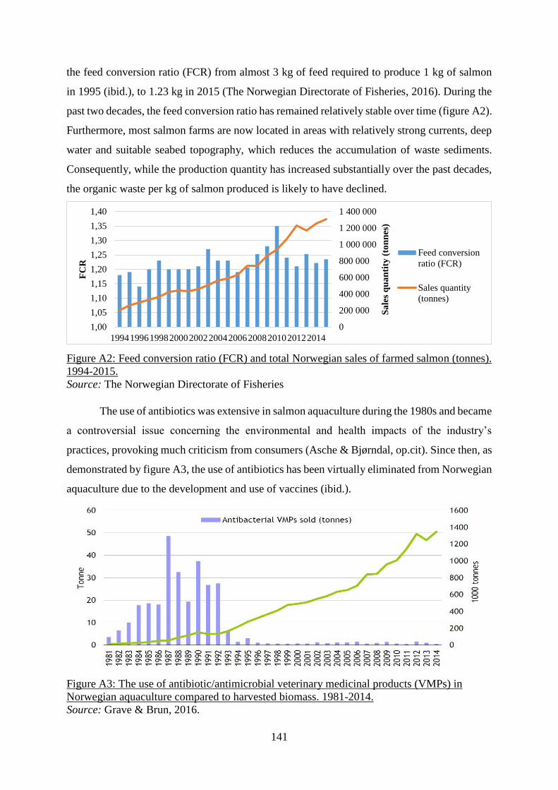
141

the feed conversion ratio (FCR) from almost 3 kg of feed required to produce 1 kg of salmon

in 1995 (ibid.), to 1.23 kg in 2015 (The Norwegian Directorate of Fisheries, 2016). During the

past two decades, the feed conversion ratio has remained relatively stable over time (figure A2).

Furthermore, most salmon farms are now located in areas with relatively strong currents, deep

water and suitable seabed topography, which reduces the accumulation of waste sediments.

Consequently, while the production quantity has increased substantially over the past decades,

the organic waste per kg of salmon produced is likely to have declined.

Figure A2: Feed conversion ratio (FCR) and total Norwegian sales of farmed salmon (tonnes).

1994-2015.


The use of antibiotics was extensive in salmon aquaculture during the 1980s and became

a controversial issue concerning the environmental and health impacts of the industry’s

practices, provoking much criticism from consumers (Asche & Bjørndal, op.cit). Since then, as

demonstrated by figure A3, the use of antibiotics has been virtually eliminated from Norwegian

aquaculture due to the development and use of vaccines (ibid.).

Figure A3: The use of antibiotic/antimicrobial veterinary medicinal products (VMPs) in

Norwegian aquaculture compared to harvested biomass. 1981-2014.

Source: Grave & Brun, 2016.

0

200 000

400 000

600 000

800 000

1 000 000

1 200 000

1 400 000

1,00

1,05

1,10

1,15

1,20

1,25

1,30

1,35

1,40

19941996199820002002200420062008201020122014

Sa

les

qu

an

tity

(to

nn

es)

FC

R

Feed conversion

ratio (FCR)

Sales quantity

(tonnes)

142

Note A2: Regulations

In 1981, the first permanent aquaculture law was established (Bjørndal, 1987). Objectives

included maintaining a small-scale, owner-operated industry structure, generating employment

in rural districts, controlling influence on the local environment and ensuring profitability, for

instance by adapting the total production to market demand (ibid.). The types of regulations

imposed on salmon grow out production can be summarised as follows: 1) regulation of entry

(licenses), 2) location of sites, 3) the size of sites (production volume), 4) factor inputs

(fingerling release), 5) structure of ownership and 6) transfer of ownership (Bjørndal, op.cit).

1991 was a turning point for the industry. The late 1980s and early 1990s had seen major

and increasing financial difficulties (Asche & Bjørndal, op.cit). Increasing supply including a

considerable increase in catches of wild salmon caused prices and profit margins to fall as

illustrated in figure 2.1, and considerable losses due to disease magnified the problems. Not

only did many farms face bankruptcy, so did the Fish Famers’ Sales Organisation (FOS), the

organisation that hitherto had been responsible for all first-hand transaction s of salmon and

trout (Asche & Bjørndal, op.cit). The government replied to the financial crisis by a major

liberalisation of the regulation regime, most importantly allowing companies to own more than

only one production licence per firm and allowing licenses to be sold in the market (ibid; Liu

et. al, 2010). As ownership regulations were abolished, firms started to merge and combine

licenses (Asche & Bjørndal, op.cit). Throughout the 1990s, mergers and more efficient

allocation of production licences led to a reduction in the number of locations, while the

production per location increased (ibid). Economies of scale was achieved by expanding farm

size, implying that the former regulatory regime had inhibited the industry from reaching the

minimum efficient scale, the size of production where all potential benefits from increasing

scale are realised. The changes contributed to ownership concentration and greater acceptance

of outside ownership in the industry (Stikholmen, op.cit).

In 1995, trade conflicts and dumping claims by the EU led to the implementation of a

new production system of feeding quotas, where the production quantity was limited by

controlling the quantities of feed that could be used per licence (Asche & Bjørndal, op.cit, 36).

The system remained in place from 1996-2003. The current MTB regime has been in operation

since 2005.

143

Table A1. Cost of production. NOK/smolt.

2008 2009 2010 2011 2012 2013 2014 2015

Roe/fingerling 1,53 1,37 1,59 1,50 1,66 1,60 1,78 1,73

Feed 0,92 0,99 1,02 1,11 1,13 1,34 1,38 1,50

Insurance 0,12 0,12 0,11 0,11 0,11 0,10 0,10 0,10

Vaccines 1,26 1,31 1,21 1,27 1,37 1,12 1,11 1,16

Labour 1,59 1,73 1,72 1,77 1,67 1,62 1,64 1,66

Depreciation 0,61 0,76 0,78 0,82 0,86 1,02 1,01 1,11

Electricity 0,43 0,44 0,51 0,53 0,45 0,51 0,49 0,45

Other operating costs 1,93 1,79 1,71 2,18 1,95 1,92 2,02 2,35

Finance cost 0,34 0,40 0,35 0,38 0,34 0,40 0,30 0,30

Cost of production per smolt 8,73 8,92 9,01 9,66 9,53 9,61 9,83 10,38

Table A2. Cost of production and cost shares, 2008 and 2015. NOK/smolt and cost shares in

percent. 2008 Cost share (2008) 2015 Cost share (2015)

Roe/fingerling 1,53 18 % 1,73 17 %

Feed 0,92 11 % 1,50 14 %

Insurance 0,12 1 % 0,10 1 %

Vaccines 1,26 14 % 1,16 11 %

Labour 1,59 18 % 1,66 16 %

Depreciation 0,61 7 % 1,11 11 %

Electricity 0,43 5 % 0,45 4 %

Other operating costs 1,93 22 % 2,35 23 %

Finance cost 0,34 4 % 0,30 3 %

Cost of production per smolt 8,73 100 % 10,38 100 %

144

APPENDIX B. BIOLOGICAL MEASURE

Note B1: The thermal growth coefficient (TGC)

Much of the biological input on fish growth is based on growth coefficients obtained from

Nofima, a research institute. Forecasting fish growth is complex as it is influenced by many

factors. The endogenous factors that are controlled by the manager at the fish plant include

stocking density, the number of juveniles released, the feeding pattern and the type of feed

(Braaten Thyholdt, 2014). If managers control these factors equally well, variations in the grow-

out period mainly results from the effects of exogenous biophysical factors on salmon

production such as sea temperature, currents, disease outbreaks and daylight hours97 (ibid.). In

particular, fish are highly reliant on temperature, and the variation in sea temperature is

considered to be the most important biophysical factor that influences salmon growth, provided

that sufficient feed and oxygen is present (ibid.). For net-pen producers these factors are mostly

outside of the farmers’ influence, whereas land based farmers may to a larger extent be able to

adapt the production environment to achieve beneficial conditions with respect to temperature,

daylight hours and currents. This analysis will not model any of these factors, but presents

assumptions about temperature along with other data in chapters IV and V.

There are several means of calculating growth in salmon, one of which is the Growth

Factor 3 (Norwegian, Vekstfaktor VF3), internationally known as the thermal growth

coefficient (TGC). After the specific growth rate (SGR), another well-known growth measure,

the TGC is perhaps the most widely used growth coefficient in aquaculture (Iversen & Kosmo,

2004; Jobling, 2003). The SGR, however, does not adjust for temperature or size differences.

As the TGC is relatively stable over large parts of the life cycle and within the usual temperature

range for salmon, the measure made it easier to compare productivity among fish groups and

across temperatures and is appropriate to use for forecasting growth (ibid.). A benefit of the

measure is that it represents a simple exponential formula that takes account both of the

temperature and fish size without relying on laborious calculations to account for different

(decreasing) daily growth rates for different (increasing) sizes of fish (Holmefjord et. al, 1994).

The TGC looks at growth directly in relation to the temperature sum and is expressed

as:

𝑇𝐺𝐶 = (𝐹𝑖𝑛𝑎𝑙 𝑤𝑒𝑖𝑔ℎ𝑡

13 − 𝑆𝑡𝑎𝑟𝑡 𝑤𝑒𝑖𝑔ℎ𝑡

13) ∗ 1000

𝐷𝑎𝑦 𝑑𝑒𝑔𝑟𝑒𝑒𝑠 ,

97 Daylight hours may be controlled through the use of artificial light.

145

where day degrees (or the temperature sum) is the temperature in degrees Celsius times the total

number of growth days. This temperature sum can be calculated by either summing every single

temperature reading or taking the average temperature for each month and multiplying these by

the number of days in each month (ibid.). The TGCs used for forecasting in this study are

obtained from Nofima and from published sources (Austreng et. al., 1987; Thorarensen &

Farrell, 2011) and are to be presented later. The formula for calculating growth using TGC is

expressed as:

𝐹𝑖𝑛𝑎𝑙 𝑤𝑒𝑖𝑔ℎ𝑡 = (𝑆𝑡𝑎𝑟𝑡 𝑤𝑒𝑖𝑔ℎ𝑡13 + 𝑇𝐺𝐶 ∗

𝐷𝑎𝑦 𝑑𝑒𝑔𝑟𝑒𝑒𝑠

1000)3

The model assumes that the TGC coefficient is independent of fish size and temperature. Some

research has indicated that the maximum difference in predicted TGC is 6% (between 50 g fish

at 4 °C and 3000 g fish at 14 °C) and the maximum difference in TGC for the same-sized fish

reared at either 4 or 14 °C is 4% (Chadwick et. al, 2010; Thorarensen & Farrell, 2011). Hence,

the model should hold fairly well within the relevant temperature range.

The temperatures assumptions in this study are as follows: 12 degrees Celsius in land

based facilities (after a smolt size of 92 g) and in sea as given below in tables B1a and b.

146

Table B1a: General assumptions about average sea temperature. Temperatures measured at a depth of 5 m at the research station of Bud,

Norway. 2006-2016 (with lots of missing data).

2006 2007 2008 2009 2010 2011 2012 2013 2014 2015 2016 Average

temperature

Number

of obs.

2006-

2016

Jan 6,528 6,08 5,407 6,0 3

Feb 6,552 5,83 5,727 4,483 4,159 5,868 6,544 5,6 7

Mar 5,535 6,487 5,37 5,39 6,119 3,723 5,661 6,012 5,93 5,6 9

Apr 5,68 6,071 6,145 4,92 5,01 3,943 6,494 5,5 7

May 6,66 7,64 8,415 10,293 6,243 6,993 8,335 6,076 7,398 7,352 8,461 7,6 11

Jun 9,703 9,267 10,373 12,475 9,513 9,21 11,317 8,954 10,1 8

Jul 13,706 12,23 13,082 11,717 12,7 4

Aug 15,509 13,997 16,331 15,72 9,28 14,387 14,928 14,3 14,3 8

Sep 14,751 10,89 15,312 14,01 12,358 14,857 13,869 15,064 13,9 8

Oct 14,25 10,297 10,455 11,319 11,308 12,245 12,552 11,8 7

Nov 9,227 8,228 9,74 9,204 8,36 10,547 10,193 9,4 7

Dec 7,387 7,695 8,405 8,987 7,939 8,1 5

Source: imr.no

147

Table B1b: Average sea temperature profile based on table 1a.

Sea

temperature

Jan 6,0

Feb 5,6

Mar 5,6

Apr 5,5

May 7,6

Jun 10,1

Jul 12,7

Aug 14,3

Sept 13,9

Oct 11,8

Nov 9,4

Dec 8,1

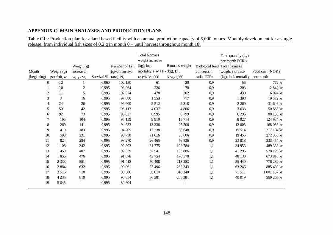
148

APPENDIX C: MAIN ANALYSES AND PRODUCTION PLANS

Table C1a: Production plan for a land based facility with an annual production capacity of 5,000 tonnes. Monthly development for a single

release, from individual fish sizes of 0.2 g in month 0 – until harvest throughout month 18.

Month

(beginning)

Weight (g)

per fish, wt

Weight (g)

increase,

wt+1 - wt Survival %

Number of fish

(given survival

rate), Nt

Total biomass

weight increase

(kg), incl.

mortality, ((wt+1 -

wt)*Nt)/1,000

Biomass weight

(kg), Bt =

Ntwt/1,000

Biological feed

conversion

ratio, FCR:

Feed quantity (kg)

per month FCR x

Total biomass

weight increase

(kg), incl. mortality

Feed cost (NOK)

per month

0 0,2 1 0,960 102 150 61 20 0,9 55 772 kr

1 0,8 2 0,995 98 064 226 78 0,9 203 2 842 kr

2 3,1 5 0,995 97 574 478 302 0,9 430 6 024 kr

3 8 16 0,995 97 086 1 553 777 0,9 1 398 19 572 kr

4 24 26 0,995 96 600 2 512 2 318 0,9 2 260 31 646 kr

5 50 42 0,995 96 117 4 037 4 806 0,9 3 633 50 865 kr

6 92 73 0,995 95 637 6 995 8 799 0,9 6 295 88 135 kr

7 165 104 0,995 95 159 9 919 15 714 0,9 8 927 124 984 kr

8 269 141 0,995 94 683 13 336 25 506 0,9 12 003 168 036 kr

9 410 183 0,995 94 209 17 238 38 648 0,9 15 514 217 194 kr

10 593 231 0,995 93 738 21 616 55 606 0,9 19 455 272 365 kr

11 824 284 0,995 93 270 26 465 76 836 0,9 23 818 333 454 kr

12 1 108 342 0,995 92 803 31 775 102 784 1,1 34 953 489 338 kr

13 1 450 407 0,995 92 339 37 541 133 886 1,1 41 295 578 129 kr

14 1 856 476 0,995 91 878 43 754 170 570 1,1 48 130 673 816 kr

15 2 333 551 0,995 91 418 50 408 213 253 1,1 55 449 776 289 kr

16 2 884 632 0,995 90 961 57 496 262 343 1,1 63 246 885 439 kr

17 3 516 718 0,995 90 506 65 010 318 240 1,1 71 511 1 001 157 kr

18 4 235 810 0,995 90 054 36 381 208 381 1,1 40 019 560 265 kr

19 5 045 - 0,995 89 604 -

426 740 1 638 847

SUM

FEEDING

(kg per

month) 448 595 6 280 324 kr

(Standing biomass, kg)

149

Table C1b: Harvest, feed and feed cost per month and per year, given the production plan as outlined in table C1a

Harvest is 22 tonnes x 19 working days in month 18:

Total harvest from a single release is the average weight per fish in

month 18 times the average number of fish throughout month 18: 416,8 tonnes

Harvest per day over 19 working days: 21,93 tonnes

Harvest per year: 5001,14 tonnes

Feed per month (tonnes): 448,6 tonnes

Feed per year (tonnes): 5 383,1 tonnes

Feed cost per month (NOK) 6 280 324 NOK

Feed cost per year (NOK) 75 363 888 NOK

Economic FCR:

1,08

150

Table C2: Production plan for a land based facility with an annual production capacity of 1,600 tonnes. Monthly development for a single

release, from individual fish sizes of 0.2 g in month 0 – until release to sea after month 8.

Month

(1st)

Weight

(g) per

fish, wt

Weight (g)

increase,

wt+1 - wt

Survival

%

Number of

fish

Total biomass

weight

increase (kg),

incl. mortality

Biological

feed

conversion

ratio, FCR:

Feed quantity

(kg) = FCR x

total biomass

weight

increase (kg)

Feed cost

(NOK)

0 0,2 0,6 0,960 1 084 287 672 0,90 605 9 075

1 0,8 2,3 0,995 1 040 915 2 394 0,90 2 155 32 320

2 3,1 4,9 0,995 1 035 711 5 075 0,90 4 567 68 512

3 8,0 16,0 0,995 1 030 532 16 489 0,90 14 840 222 595

4 24,0 26,0 0,995 1 025 379 26 660 0,90 23 994 359 908

5 50,0 42,0 0,995 1 020 253 42 851 0,90 38 566 578 483

6 92,0 73,1 0,995 1 015 151 74 248 0,90 66 823 1 002 350

7 165,1 104,2 0,995 1 010 076 105 291 0,90 94 762 1 421 426

8 269,4 140,9 0,995 1 005 025 141 559 0,90 127 403 1 911 045

9 410,2 1 000 000 0 -

SUM: 373 714 5 605 715

Economic

FCR: 0,91

Hatcery survival rate: 0,9 Price per kg of feed: 15

Number of roe purchases: 4 Price per egg 1

Egg quantity per batch of roe 120 4763

151

Table C3: Investment and reinvestment used to estimate terminal value of investment, chapter

IV:

Investment and

reinvestment

Year 20 398558

Year 29 6 011

Year 40 398558

Year 49 6 011

Year 60 398558

152

Table C4: 410-g grow-out. Average production time from release until harvest of 5-kg

salmon. Estimated based on four annual releases in December, March, June and September

Month December March June Sept Average

0 410 410 410 410 410

1 479 473 565 553 517

2 567 594 837 720 680

3 665 785 1174 890 879

4 772 1078 1522 1032 1101

5 939 1486 1843 1177 1361

6 1194 1970 2155 1335 1664

7 1576 2455 2408 1502 1985

8 2095 2893 2660 1759 2352

9 2697 3310 2929 2141 2769

10 3291 3645 3209 2695 3210

11 3820 3976 3630 3426 3713

12 4320 4327 4241 4252 4285

13 4719 4689 5101 5048 4889

14 5112 5227 5747 5362

153

Table C5a: Production time from release to harvest, 100-g smolts. Releases in May and

October (as illustrated in the text, figure 6.1).

Month

(beginning)

Weight (g) per fish

May October

0 100 100

1 150 145

2 254 207

3 421 262

4 640 322

5 877 390

6 1103 465

7 1326 585

8 1510 775

9 1696 1065

10 1896 1470

11 2107 1951

12 2427 2433

13 2897 2867

14 3570 3282

15 4445 3615

16 5421 3945

17 4294

18 4923

The production time for grow-out of 100-g smolts released in the remaining months of a year

is given below in table C4b.

154

Table C5b: Weight development in grams per fish by month of release to sea (smolt, 100 g). January – December.

Month January February March April May June July August Sept October November December

0 100 100 100 100 100 100 100 100 100 100 100 100

1 126 126 125 136 150 164 174 172 159 145 139 128

2 163 162 177 212 254 292 302 276 236 207 181 166

3 206 224 267 342 421 468 450 384 319 262 229 210

4 278 327 416 541 640 662 597 498 392 322 283 260

5 396 496 641 798 877 850 748 595 469 390 344 344

6 586 747 927 1070 1103 1039 875 697 556 465 444 479

7 865 1061 1226 1326 1326 1196 1005 809 651 585 602 693

8 1209 1387 1505 1577 1510 1356 1147 929 800 775 850 1002

9 1563 1690 1778 1783 1696 1529 1299 1117 1031 1065 1202 1380

10 1890 1984 2001 1991 1896 1712 1532 1403 1378 1470 1625 1766

11 2207 2224 2225 2213 2107 1991 1882 1826 1855 1951 2053 2119

12 2463 2463 2464 2447 2427 2406 2393 2396 2413 2433 2443 2460

13 2720 2719 2715 2799 2897 3002 3070 3052 2965 2867 2817 2736

14 2993 2986 3092 3315 3570 3786 3839 3695 3460 3282 3118 3010

15 3277 3387 3642 4049 4445 4666 4585 4265 3929 3615 3417 3302

16 3703 3971 4422 4998 5421 5512 5241 4803 4303 3945 3734 3605

17 4322 4796 5426 6050 6353 6252 5856 5231 4673 4294 4063 4059

18 5193 5854 6536 7051 7166 6942 6343 5651 5063 4654 4553 4716

19 6306 7020 7588 7921 7921 7487 6821 6092 5464 5190 5262 5637

155

Table C6: Weight development in grams per fish by month of release to sea (post smolt, 410 g). January – December.

Month January February March April May June July August Sept October November December

0 410 410 410 410 410 410 410 410 410 410 410 410

1 474 474 473 499 531 565 587 581 553 521 505 479

2 562 559 594 670 759 837 857 804 720 659 603 567

3 657 695 785 935 1087 1174 1142 1017 890 776 705 665

4 807 906 1078 1308 1484 1522 1409 1229 1032 896 818 772

5 1039 1226 1486 1755 1889 1843 1670 1404 1177 1028 940 939

6 1389 1669 1970 2205 2258 2155 1884 1582 1335 1169 1130 1194

7 1868 2190 2455 2613 2613 2408 2099 1773 1502 1387 1417 1576

8 2428 2709 2893 3003 2900 2660 2329 1975 1759 1716 1843 2095

9 2982 3176 3310 3318 3185 2929 2571 2281 2141 2196 2416 2697

10 3478 3619 3645 3629 3488 3209 2934 2734 2695 2838 3076 3291

11 3949 3974 3976 3959 3802 3630 3467 3381 3426 3569 3722 3820

12 4325 4325 4327 4301 4271 4241 4222 4227 4252 4280 4295 4320

13 4696 4695 4689 4810 4951 5101 5197 5172 5048 4908 4836 4719

14 5087 5078 5227 5543 5901 6202 6276 6076 5747 5497 5265 5112

156

Table C7: The simulation model using 410-gram smolt. Weight per fish at each location, survival rate, number of fish per location, total biomass

and MTB balance and harvest in number of fish per location.

Month

(IB)

Location

1

Location

2

Location

3

Location

4

Location

5

Location

6 Release per batchMortality

Location

1

Location

2

Location

3

Location

4

Location

5

Location

6 IB biomass

SUM Net

growth

forecast

current

month

Target IB

biomass =

MTB - net

growth

forecast

IB biomass

balance Location 1 Location 2

Location

3

Location

4

Location

5

Location

6

Harvest,

number

of fish

Harvesr

at UB

weight

Weight per fish (kg) Number of fish (IB = IB Survived fish after last month - harvest previous month) Harvest (number)

0 0 0 0 0 0

Mar 0,410 500 000 0,75 % 500 000 205 000 29 567 3 090 433 2 885 433 0 0 0 0 0 0 0 0

Apr 0,473 496 250 234 567 58 116 3 061 884 2 827 317 0 0 0 0 0 0 0 0

May 0,594 492 528 292 683 91 140 3 028 860 2 736 176 0 0 0 0 0 0 0 0

Jun 0,785 488 834 383 824 139 091 2 980 909 2 597 085 0 0 0 0 0 0 0 0

Jul 1,078 0,410 485 168 500 000 727 915 279 015 2 840 985 2 113 070 0 0 0 0 0 0 0 0

Aug 1,486 0,587 481 529 496 250 1 006 930 356 791 2 763 209 1 756 279 0 0 0 0 0 0 0 0

Sept 1,970 0,857 477 918 492 528 1 363 721 359 011 2 760 989 1 397 267 0 0 0 0 0 0 0 0

Oct 2,455 1,142 474 333 488 834 1 722 733 322 503 2 797 497 1 074 765 0 0 0 0 0 0 0 0

Nov 2,893 1,409 0,410 470 776 485 168 500 000 2 250 235 351 099 2 768 901 518 666 0 0 0 0 0 0 0 0

Dec 3,310 1,670 0,505 467 245 481 529 496 250 2 601 334 286 400 2 833 600 232 266 12 870 0 0 0 0 0 12 870 46 909

Jan 3,645 1,884 0,603 450 871 477 918 492 528 2 840 826 279 117 2 840 883 57 68 800 0 0 0 0 0 68 800 273 574

Feb 3,976 2,099 0,705 378 689 474 333 488 834 2 846 369 273 507 2 846 493 124 111 250 0 0 0 0 0 111 250 481 328

Mar 4,327 2,329 0,818 0,410 264 599 470 776 485 168 500 000 2 843 547 276 335 2 843 665 118 84 000 0 0 0 0 0 84 000 393 867

Apr 4,689 2,571 0,940 0,473 178 614 467 245 481 529 496 250 2 726 015 393 935 2 726 065 50 98 660 0 0 0 0 0 98 660 515 725

May 5,227 2,934 1,130 0,594 78 615 463 741 477 918 492 528 2 604 225 515 768 2 604 232 8 78 025 47 500 0 0 0 0 125 525 632 981

Jun 6,002 3,467 1,417 0,785 0 412 763 474 333 488 834 2 487 012 632 948 2 487 052 40 0 218 880 0 0 0 0 218 880 924 062

Jul 7,079 4,222 1,843 1,078 0,410 0 190 787 470 776 485 168 500 000 2 400 897 719 005 2 400 995 97 0 136 440 0 0 0 0 136 440 709 017

Aug 8,439 5,197 2,416 1,486 0,587 0 52 916 467 245 481 529 496 250 2 410 885 709 063 2 410 937 52 0 52 519 85 510 0 0 0 138 029 592 665

Sept 6,276 3,076 1,970 0,857 0 0 378 231 477 918 492 528 2 527 281 592 714 2 527 286 5 0 0 123 300 0 0 0 123 300 458 937

Oct 7,301 3,722 2,455 1,142 0 252 094 474 333 488 834 2 661 057 458 892 2 661 108 51 0 0 142 150 0 0 0 142 150 610 585

Nov 8,191 4,295 2,893 1,409 0,410 0 108 053 470 776 485 168 500 000 2 714 364 405 547 2 714 453 89 0 0 62 800 0 0 0 62 800 303 671

Dec 9,015 4,836 3,310 1,670 0,505 0 44 443 467 245 481 529 496 250 2 816 240 303 728 2 816 272 32 0 0 44 109 12 870 0 0 56 979 279 139

Jan 5,265 3,645 1,884 0,603 0 0 450 871 477 918 492 528 2 840 828 279 117 2 840 883 54 0 0 0 68 800 0 0 68 800 273 574

Feb 5,687 3,976 2,099 0,705 0 378 689 474 333 488 834 2 846 372 273 507 2 846 493 122 0 0 0 111 250 0 0 111 250 481 328

Mar 0,410 6,130 4,327 2,329 0,818 500 000 0 264 599 470 776 485 168 2 843 550 276 335 2 843 665 114 0 0 0 84 000 0 0 84 000 393 867

Apr 0,473 6,586 4,689 2,571 0,940 496 250 0 178 614 467 245 481 529 2 726 018 393 935 2 726 065 47 0 0 0 98 660 0 0 98 660 515 725

May 0,594 5,227 2,934 1,130 492 528 0 78 615 463 741 477 918 2 604 225 515 768 2 604 232 8 0 0 0 78 025 47 500 0 125 525 632 981

Jun 0,785 6,002 3,467 1,417 488 834 0 412 763 474 333 2 487 012 632 948 2 487 052 40 0 0 0 0 218 880 0 218 880 924 062

Jul 1,078 0,410 7,079 4,222 1,843 485 168 500 000 0 190 787 470 776 2 400 897 719 005 2 400 995 97 0 0 0 0 136 440 0 136 440 709 017

Aug 1,486 0,587 8,439 5,197 2,416 481 529 496 250 0 52 916 467 245 2 410 885 709 063 2 410 937 52 0 0 0 0 52 519 85 510 138 029 592 665

Sept 1,970 0,857 6,276 3,076 477 918 492 528 0 0 378 231 2 527 281 592 714 2 527 286 5 0 0 0 0 0 123 300 123 300 458 937

Oct 2,455 1,142 7,301 3,722 474 333 488 834 0 252 094 2 661 057 458 892 2 661 108 51 0 0 0 0 0 142 150 142 150 610 585

Nov 2,893 1,409 0,410 8,191 4,295 470 776 485 168 500 000 0 108 053 2 714 364 405 547 2 714 453 89 0 0 0 0 0 62 800 62 800 303 671

Dec 3,310 1,670 0,505 9,015 4,836 467 245 481 529 496 250 0 44 443 2 816 240 303 728 2 816 272 32 12 870 0 0 0 0 44 109 56 979 279 139

Jan 3,645 1,884 0,603 5,265 450 871 477 918 492 528 0 0 2 840 828 279 117 2 840 883 54 68 800 0 0 0 0 0 68 800 273 574

Feb 3,976 2,099 0,705 5,687 378 689 474 333 488 834 0 2 846 372 273 507 2 846 493 122 111 250 0 0 0 0 0 111 250 481 328

Mar 4,327 2,329 0,818 0,410 6,130 264 599 470 776 485 168 500 000 0 2 843 550 276 335 2 843 665 114 84 000 0 0 0 0 0 84 000 393 867

Apr 4,689 2,571 0,940 0,473 6,586 178 614 467 245 481 529 496 250 0 2 726 018 393 935 2 726 065 47 98 660 0 0 0 0 0 98 660 515 725

May 5,227 2,934 1,130 0,594 78 615 463 741 477 918 492 528 0 2 604 225 515 768 2 604 232 8 78 025 47 500 0 0 0 0 125 525 632 981

Jun 6,002 3,467 1,417 0,785 0 412 763 474 333 488 834 2 487 012 632 948 2 487 052 40 0 218 880 0 0 0 0 218 880 924 062

Jul 7,079 4,222 1,843 1,078 0,410 0 190 787 470 776 485 168 500 000 2 400 897 719 005 2 400 995 97 0 136 440 0 0 0 0 136 440 709 017

Aug 8,439 5,197 2,416 1,486 0,587 0 52 916 467 245 481 529 496 250 2 410 885 709 063 2 410 937 52 0 52 519 85 510 0 0 0 138 029 592 665

Sept 0,000 6,276 3,076 1,970 0,857 0 0 378 231 477 918 492 528 2 527 281 592 714 2 527 286 5 0 0 123 300 0 0 0 123 300 458 937

Oct 0,000 7,301 3,722 2,455 1,142 0 252 094 474 333 488 834 2 661 057 458 892 2 661 108 51 0 0 142 150 0 0 0 142 150 610 585

Nov 0,000 8,191 4,295 2,893 1,409 0,410 0 108 053 470 776 485 168 500 000 2 714 364 405 547 2 714 453 89 0 0 62 800 0 0 0 62 800 303 671

Dec 0,000 9,015 4,836 3,310 1,670 0,505 0 44 443 467 245 481 529 496 250 2 816 240 303 728 2 816 272 32 0 0 44 109 12 870 0 0 56 979 279 139

Jan 0,000 0,000 5,265 3,645 1,884 0,603 0 450 871 477 918 492 528 2 840 828 279 117 2 840 883 54 0 0 0 68 800 0 0 68 800 273 574

Feb 0,000 0,000 5,687 3,976 2,099 0,705 0 378 689 474 333 488 834 2 846 372 273 507 2 846 493 122 0 0 0 111 250 0 0 111 250 481 328

Mar 0,410 0,000 6,130 4,327 2,329 0,818 500 000 0 264 599 470 776 485 168 2 843 550 276 335 2 843 665 114 0 0 0 84 000 0 0 84 000 393 867

Apr 0,473 0,000 6,586 4,689 2,571 0,940 496 250 0 178 614 467 245 481 529 2 726 018 393 935 2 726 065 47 0 0 0 98 660 0 0 98 660 515 725

May 0,594 0,000 0,000 5,227 2,934 1,130 492 528 78 615 463 741 477 918 2 604 225 515 768 2 604 232 8 0 0 0 78 025 47 500 0 125 525 632 981

Jun 0,785 0,000 0,000 6,002 3,467 1,417 488 834 0 412 763 474 333 2 487 012 632 948 2 487 052 40 0 0 0 0 218 880 0 218 880 924 062

157

Table C8: The simulation model using 100-gram smolt. Weight per fish at each location, survival rate, number of fish per location, total biomass

and MTB balance and harvest in number of fish per location.

Month

(IB) Loc. 1 Loc. 2 Loc. 3 Loc. 4 Loc. 5 Loc. 6 Release per batchMortality Loc. 1 Loc. 2 Loc. 3 Loc. 4 Loc. 5 Loc. 6 IB biomass

Net growth

forecast

current

month

Target IB

biomass =

MTB - net

growth

forecast

IB biomass

balance Loc. 1 Loc. 2 Loc. 3 Loc. 4 Loc. 5 Loc. 6

Harvest,

number

of fish

Harvesr

at UB

weight

Weight per fish (kg) Number of fish (IB = IB Survived fish after last month - harvest previous month) Harvest (number)

0 0 0 0 0 0

Mar 0,100 500 000 0,75 % 500 000 50 000 12 119 3 107 881 3 057 881 0 0 0 0 0 0 0 0

Apr 0,125 496 250 62 119 25 303 3 094 697 3 032 578 0 0 0 0 0 0 0 0

May 0,177 492 528 87 422 43 027 3 076 973 2 989 551 0 0 0 0 0 0 0 0

Jun 0,267 488 834 130 449 71 421 3 048 579 2 918 130 0 0 0 0 0 0 0 0

Jul 0,416 0,100 485 168 500 000 251 870 143 507 2 976 493 2 724 623 0 0 0 0 0 0 0 0

Aug 0,641 0,174 481 529 496 250 395 377 196 349 2 923 651 2 528 274 0 0 0 0 0 0 0 0

Sept 0,927 0,302 477 918 492 528 591 726 209 968 2 910 032 2 318 306 0 0 0 0 0 0 0 0

Oct 1,226 0,450 474 333 488 834 801 694 196 926 2 923 074 2 121 380 0 0 0 0 0 0 0 0

Nov 1,505 0,597 0,100 470 776 485 168 500 000 1 048 620 211 291 2 908 709 1 860 089 0 0 0 0 0 0 0 0

Dec 1,778 0,748 0,139 467 245 481 529 496 250 1 259 911 175 634 2 944 366 1 684 455 0 0 0 0 0 0 0 0

Jan 2,001 0,875 0,181 463 741 477 918 492 528 1 435 545 177 097 2 942 903 1 507 358 0 0 0 0 0 0 0 0

Feb 2,225 1,005 0,229 460 263 474 333 488 834 1 612 642 190 646 2 929 354 1 316 712 0 0 0 0 0 0 0 0

Mar 2,464 1,147 0,283 0,100 456 811 470 776 485 168 500 000 1 853 288 212 527 2 907 473 1 054 186 0 0 0 0 0 0 0 0

Apr 2,715 1,299 0,344 0,125 453 385 467 245 481 529 496 250 2 065 814 335 442 2 784 558 718 743 0 0 0 0 0 0 0 0

May 3,092 1,532 0,444 0,177 449 984 463 741 477 918 492 528 2 401 257 507 973 2 612 027 210 771 121 900 0 0 0 0 0 121 900 443 989

Jun 3,642 1,882 0,602 0,267 324 709 460 263 474 333 488 834 2 465 241 654 697 2 465 303 62 179 050 0 0 0 0 0 179 050 791 700

Jul 4,422 2,393 0,850 0,416 0,100 143 224 456 811 470 776 485 168 500 000 2 378 238 741 711 2 378 289 51 134 900 0 0 0 0 0 134 900 731 953

Aug 5,426 3,070 1,202 0,641 0,174 7 250 453 385 467 245 481 529 496 250 2 387 995 731 932 2 388 068 73 7 195 148 200 0 0 0 0 155 395 616 018

Sept 6,536 3,839 1,625 0,927 0,302 0 301 784 463 741 477 918 492 528 2 503 909 616 015 2 503 985 76 0 106 250 0 0 0 0 106 250 487 106

Oct 7,588 4,585 2,053 1,226 0,450 0 193 271 460 263 474 333 488 834 2 632 818 487 135 2 632 865 47 0 91 530 0 0 0 0 91 530 479 716

Nov 8,501 5,241 2,443 1,505 0,597 0,100 100 291 456 811 470 776 485 168 500 000 2 690 234 429 721 2 690 279 45 0 54 850 0 0 0 0 54 850 321 218

Dec 5,856 2,817 1,778 0,748 0,139 44 689 453 385 467 245 481 529 496 250 2 798 736 321 222 2 798 778 42 0 44 354 5 600 0 0 0 49 954 298 812

Jan 6,343 3,118 2,001 0,875 0,181 0 444 384 463 741 477 918 492 528 2 821 146 298 691 2 821 309 163 0 0 85 800 0 0 0 85 800 293 203

Feb 6,821 3,417 2,225 1,005 0,229 0 355 251 460 263 474 333 488 834 2 826 634 293 310 2 826 690 55 0 0 91 200 0 0 0 91 200 340 566

Mar 0,100 7,320 3,734 2,464 1,147 0,283 500 000 261 387 456 811 470 776 485 168 2 829 379 290 537 2 829 463 84 0 0 100 400 0 0 0 100 400 407 945

Apr 0,125 4,063 2,715 1,299 0,344 496 250 159 026 453 385 467 245 481 529 2 711 971 407 973 2 712 027 56 0 0 117 500 0 0 0 117 500 535 030

May 0,177 4,553 3,092 1,532 0,444 492 528 40 334 449 984 463 741 477 918 2 584 914 534 945 2 585 055 141 0 0 40 031 121 900 0 0 161 931 654 617

Jun 0,267 5,262 3,642 1,882 0,602 488 834 0 324 709 460 263 474 333 2 465 242 654 697 2 465 303 61 0 0 0 179 050 0 0 179 050 791 700

Jul 0,416 0,100 6,250 4,422 2,393 0,850 485 168 500 000 0 143 224 456 811 470 776 2 378 240 741 711 2 378 289 49 0 0 0 134 900 0 0 134 900 731 953

Aug 0,641 0,174 7,506 5,426 3,070 1,202 481 529 496 250 7 250 453 385 467 245 2 387 995 731 932 2 388 068 73 0 0 0 7 195 148 200 0 155 395 616 018

Sept 0,927 0,302 6,536 3,839 1,625 477 918 492 528 0 301 784 463 741 2 503 909 616 015 2 503 985 76 0 0 0 0 106 250 0 106 250 487 106

Oct 1,226 0,450 7,588 4,585 2,053 474 333 488 834 0 193 271 460 263 2 632 818 487 135 2 632 865 47 0 0 0 0 91 530 0 91 530 479 716

Nov 1,505 0,597 0,100 8,501 5,241 2,443 470 776 485 168 500 000 100 291 456 811 2 690 234 429 721 2 690 279 45 0 0 0 0 54 850 0 54 850 321 218

Dec 1,778 0,748 0,139 5,856 2,817 467 245 481 529 496 250 44 689 453 385 2 798 736 321 222 2 798 778 42 0 0 0 0 44 354 5 600 49 954 298 812

Jan 2,001 0,875 0,181 6,343 3,118 463 741 477 918 492 528 0 444 384 2 821 146 298 691 2 821 309 163 0 0 0 0 0 85 800 85 800 293 203

Feb 2,225 1,005 0,229 6,821 3,417 460 263 474 333 488 834 0 355 251 2 826 634 293 310 2 826 690 55 0 0 0 0 0 91 200 91 200 340 566

Mar 2,464 1,147 0,283 0,100 7,320 3,734 456 811 470 776 485 168 500 000 261 387 2 829 379 290 537 2 829 463 84 0 0 0 0 0 100 400 100 400 407 945

Apr 2,715 1,299 0,344 0,125 4,063 453 385 467 245 481 529 496 250 159 026 2 711 971 407 973 2 712 027 56 0 0 0 0 0 117 500 117 500 535 030

May 3,092 1,532 0,444 0,177 4,553 449 984 463 741 477 918 492 528 40 334 2 584 914 534 945 2 585 055 141 121 900 0 0 0 0 40 031 161 931 654 617

Jun 3,642 1,882 0,602 0,267 5,262 324 709 460 263 474 333 488 834 0 2 465 242 654 697 2 465 303 61 179 050 0 0 0 0 0 179 050 791 700

Jul 4,422 2,393 0,850 0,416 0,100 6,250 143 224 456 811 470 776 485 168 500 000 0 2 378 240 741 711 2 378 289 49 134 900 0 0 0 0 0 134 900 731 953

Aug 5,426 3,070 1,202 0,641 0,174 7,506 7 250 453 385 467 245 481 529 496 250 2 387 995 731 932 2 388 068 73 7 195 148 200 0 0 0 0 155 395 616 018

Sept 6,536 3,839 1,625 0,927 0,302 0 301 784 463 741 477 918 492 528 2 503 909 616 015 2 503 985 76 0 106 250 0 0 0 0 106 250 487 106

Oct 7,588 4,585 2,053 1,226 0,450 0 193 271 460 263 474 333 488 834 2 632 818 487 135 2 632 865 47 0 91 530 0 0 0 0 91 530 479 716

Nov 8,501 5,241 2,443 1,505 0,597 0,100 100 291 456 811 470 776 485 168 500 000 2 690 234 429 721 2 690 279 45 0 54 850 0 0 0 0 54 850 321 218

Dec 0,000 5,856 2,817 1,778 0,748 0,139 44 689 453 385 467 245 481 529 496 250 2 798 736 321 222 2 798 778 42 0 44 354 5 600 0 0 0 49 954 298 812

Jan 0,000 6,343 3,118 2,001 0,875 0,181 0 444 384 463 741 477 918 492 528 2 821 146 298 691 2 821 309 163 0 0 85 800 0 0 0 85 800 293 203

Feb 0,000 6,821 3,417 2,225 1,005 0,229 0 355 251 460 263 474 333 488 834 2 826 634 293 310 2 826 690 55 0 0 91 200 0 0 0 91 200 340 566

Mar 0,100 7,320 3,734 2,464 1,147 0,283 500 000 261 387 456 811 470 776 485 168 2 829 379 290 537 2 829 463 84 0 0 100 400 0 0 0 100 400 407 945

Apr 0,125 0,000 4,063 2,715 1,299 0,344 496 250 159 026 453 385 467 245 481 529 2 711 971 407 973 2 712 027 56 0 0 117 500 0 0 0 117 500 535 030

May 0,177 0,000 4,553 3,092 1,532 0,444 492 528 40 334 449 984 463 741 477 918 2 584 914 534 945 2 585 055 141 0 0 40 031 121 900 0 0 161 931 654 617

OF LAND BASED FARMING OF SALMON: ECONOMIC …

Documents

Transcript of OF LAND BASED FARMING OF SALMON: ECONOMIC …