I6The Originand Developmentof LaboratoryModels andAnalogues of theOcean Circulation

Alan . Faller

16.1 A Brief Philosophy of LaboratoryExperimentation

"No one believes a theory, except the theorist. Every-one believes an experiment--except the experimen-ter." This often used adage, although not aways accu-rate in detail, carries a certain element of truth. Herewe consider certain experiments-analogs, models, orfundamental studies of basic fluid dynamics-that areintended to be relevant to one or another aspect of theocean circulation. These are physical, fluid models-asopposed to numerical, analytical, abstract, or conceptualmodels-that make use of a real fluid. When the fluidin a container is subjected to some driving force, thefluid moves. It is observed by the experimenter. It isthere. It is a real fluid circulation. Apart from its rele-vance, why should it not be believed?

The experienced experimenter is well aware of thepitfalls of his trade. Aside from the accuracy of hisreported observations there are many questions. Werethe boundary conditions well controlled? Were thephysical properties of the materials and their variationsduring the experiment known? Did the methods ofobservation (probes, dyes, tracers, lighting) influencethe results? Were the reported observations complete,or at least representative? or were they filtered, mas-saged, interpreted, selectively reported, etc.? In factthere is always an element of judgment, selectivity,and interpretation concerning what to observe, andhaving observed, what to record, and what to report.Thus, despite the apparent confidence that may be ex-uded in publication, the cautious experimenter main-tains a restraint born of continual reflection on theextensive preparations necessary for an apparently sim-ple experiment and the many opportunities for errorand misinterpretation.

We can broadly classify experiments into four cate-gories, according to their intent, under these headings:(1) simulation, (2) abstraction, (3) verification, and (4)extension. In the first category the experimenter at-tempts to represent nature in miniature in so far aspossible. An effort is made to include all of the relevantdriving mechanisms, and the geometry is scaled as innature, although some distortion may be necessary.Using theoretical guides such as the matching of theappropriate nondimensional ratios, the intent is tolearn by trial and error to what extent the ocean cir-culation can be reproduced as a scale model. If it werepossible to reproduce known features of the North At-lantic circulation, for example, such a model could beused to predict similarly scaled features of the oceancirculation in less accessible regions of the world. Thepredictions would serve as a guide to further explora-tion and would be compared with observations as theybecame available. The simulation mode of experimen-

462Alan J. Faller

tation is appealing to the eye of the layman who canrather easily be convinced of its possible applicationand relevance.

The second mode of experimentation is rather likeabstract art. The artist draws out (abstracts) from somenatural subject those features that he imagines to be ofsignificance, and he displays his interpretation of thosefeatures on canvas or in stone for the reaction of hispeers and his public. The experimental scientist con-ceptually isolates one or more processes that he be-lieves to be significant in nature, and he displays andtests them in the form of an operational laboratoryexperiment. Just as it may be difficult for the artist topersuade his lay audience of the sincerity of his efforts(although his fellow artists understand), so also thescientist may have difficulty convincing his nonprofes-sional audience that his experiment is relevant to thegrand scheme of things past, present, and future.

Abstract experiments may be particularly successfulin systems that can be decomposed linearly withoutdoing violence to the essential dynamics, i.e., systemsin which the abstracted phenomenon can be isolatedby virtue of a lack of coupling with other processes.This may be possible because of a smallness of ampli-tude of potentially interactive processes, or because ofmismatch in the temporal and spatial scales of thevarious processes. But even in those situations wheredecomposition is not warranted, one can say, "If ....Perhaps a planet will be found where these conditionsprevail; or perhaps some machinery in a chemicalplant, somewhere, generates the conditions that I amstudying; or perhaps I can build upon this experimentto incorporate the interactive processes necessary fora more realistic representation of the oceanic circula-tion (simulation?). In any case I will publish my ab-stract results for the benefit of posterity."

Abstraction experiments, in contrast to direct sim-ulation, are more readily subject to a posteriori math-ematical analysis because of their relative simplicity.They may more directly lead to the advancement oftheoretical aspects of the problem. Either mode maybe regarded as exploratory, for it is likely that certainnew aspects of the fluid circulations will emerge thatwere not anticipated and that will require rationaliza-tion. Here again the abstract experiment has the ad-vantage of its simplicity, for deviations from the antic-ipated behavior will be more clearly recognized. Thesimulation experiment, however, will generally pose alarger variety of unanticipated phenomena because ofits inherently greater complexity.

The verification mode of laboratory experiment im-plies an apparatus designed to test and verify) a specificanalytical or numerical model. A certain theoreticalmodel predicts a steady-state circulation, the temporal

development of a flow, or perhaps an instability. Ap-paratus is designed to match the conditions of the the-ory in so far as possible, and, as often as not, the theoryis modified to conform to the limitations of the exper-iment. But in all cases under this category there is adetailed theory capable of a priori predictions and thephysical conditions of the theory and of the experimentare closely matched. If this matching is sufficientlyprecise, the experiment will exactly verify the predic-tions. From this viewpoint the situation may at firstappear to be rather sterile, but this is not the case atall. For following the adage, "No one believes a the-ory ... ; everyone believes an experiment .. ," wefind that the theorist has arrived. For now everyonebelieves the theory, and rightly so, because it is con-firmed by the experiment! The verification mode oflaboratory experiment is widely endorsed by theorists.

The fourth type of experiment is the extension mode.The experimenter, having set up the theorist by col-laboration and verification of his theory, now attemptsto do him in by varying the parameters of the experi-ments, and 8, until they lie outside the range ofvalidity of the theory. It is then incumbent upon thetheorist to expand everything in powers of and 8 totake into account the nonlinear aspects of the flow,but here the experimenter always has the upper handand can easily keep one step ahead of the theorist. Itis only necessary to do this in a manner in keepingwith accepted scientific and engineering practice, ex-pressing the experimental results in terms of the min-imum number of nondimensional ratios appropriate tothe case at hand. Oftentimes, of course, the experi-menter and the theorist are one and the same person.

This short excursion into the philosophy of labora-tory experimentation may be found useful in the in-terpretation of the remainder of this chapter. Perhapsnot all experimental studies are cleary motivated andcan be identified as belonging exclusively to one or theother of the categories discussed above, but such aclassification seems to be by and large appropriate.

16.2 Introduction

Perhaps the first rotating laboratory experiment spe-cifically directed toward understanding some aspect ofthe ocean circulation was that of C. A. Bjerknes in1902, as reported by Ekman (1905). Because this reportis not well known and because a discussion of its re-sults will have later application, I have reproduced ithere:

The late Prof. C. A. Bjerknes at Kristiania, whose vividinterest seems to have been bestowed on every exten-sion of knowledge in his branch, also made in theautumn of 1902, some experiments with the object ofverifying some of the results to be found in Section 1of this paper.

463Laboratory Models of Ocean Circulation

His apparatus consisted of a low cylinder (12 or17 cm. high and 36 or 44 cm. wide) made of metal orglass, and resting on a table which could be put intouniform rotation (about 7 turns a minute against thesun) by means of a water-turbine. To the upper edge ofthe rotating cylinder was attached a jet having a hori-zontal split, 10 cm. long and 1 mm. broad; and throughthis a stream of air was forced from a pump to producea wind diametrically across the cylinder over a 10 cm.broad belt.

The motion of the water was observed by means ofsmall balls which just floated in it. As a result of therotation of the cylinder the current always swept to-wards the right and thus formed a large whirl-pooloccupying, when seen in the wind's direction, the mid-dle as well as the right half of the cylinder.

The direction of motion at different depths was ob-served at the centre of the cylinder, on a sensitive vane(4 cm. long and 1 mm. high) which could be raised andlowered during the experiment without disturbing themotion. The direction of the vane was read against aglass square divided into radians and laid on top of thecylinder. The following table taken from Prof. Bjerknes'note-book kept in his laboratory gives as an examplea series of measurements made during such an exper-iment. The first column gives the depth in cm. belowthe surface, the second column the deviation of thecurrent to the right or left of the wind's direction.

Surface (cm)0.511.522.533.544.555.566.57

20-25° right45-50° "45-50° "25-30° "0-100 "

0o .

5-10° left5-10° "5-10° "

100 "10- 15° "15-20° "

20° "20° "

20-25o ,,

The circumstances under which these experimentswere made were in any case such as to satisfy theconditions for stationary motion but very roughly; andan exact interpretation may furthermore be difficultowing to the shape of the vessel, etc. It is certain how-ever that their real object was to obtain merely quali-tative verification of the reality of the phenomena con-sidered, and as such they are very striking andinstructive. Both the deflection of the surface-currentand the increase of the angle of deflection increasesonly in the very uppermost layer; and this is explainedas a result of the rapid rotation of the vessel. Indeed avalue of /u = 0.3 (which would not appear to be toosmall for motion on such a small scale) would giveDEk = 2 cm only. [Author's note: Here I have used DEkin place of D to avoid later confusion. As used here andin other recent literature D = DEk/ir is the mathemat-ically more convenient measure of boundary-layerthickness.] The directions of motion below this levelhave very much the appearance of a "midwater-cur-rent" produced by a pressure-gradient.

Apparently Ekman determined the effective viscos-ity tx = 0.3 indirectly from his estimate DEk = 2 cm,for with a rotation rate l = 0.73 s- l and with theviscosity of water = 0.01 we find DEk = 0.37 cm andD = 0.117 cm. Thus the laminar Ekman depth wouldbe considerably shallower than that inferred from theexperimental data, as Ekman must have recognized.Departing temporarily from the historical developmentto consider this question, these early results possiblymay be explained in the light of recent laboratory ex-periments and numerical calculations on the stabilityof the Ekman boundary layer.

Laboratory studies have mostly been confined toflow over a rigid boundary (Faller, 1963; Faller andKaylor, 1967; Tatro and Mollo-Christensen, 1967;Caldwell and van Atta, 1970; Cerasoli, 1975), and mostcomparative theoretical studies also have been con-cerned with the rigid-boundary case.

The Reynolds number for the Ekman layer is definedas Re = UD/, where U is the difference between thespeed at the boundary and the speed of the interiorflow. Over a rigid boundary the critical value for in-stability is approximately Re = 55. For the Ekmanlayer with a free boundary, the profile of flow is exactlythe same, but potential instabilities are not constrainedby a no-slip boundary condition. A preliminary esti-mate given by Faller and Kaylor (1967) was Re =12 + 3 for the first onset of instability. This result hasrecently been confirmed with a more accurate calcu-lation by Iooss, Nielsen, and True (1978), who foundRe, = 11.816. In C. A. Bjerknes's experiment the cor-responding critical surface water speed would be ap-proximately U = 1 cm s- 1, and the corresponding crit-ical wind stress would be r = 0.12 dyncm-2 . Stillanother possibility is that of Langmuir circulations, asubject that will be touched upon briefly later, insection 16.6.10 and in this connection it would beinteresting to know whether the air jet had sufficientspeed to raise capillary waves. Unfortunately Ekman'saccount gives no means of estimating the air or waterspeeds, but it seems likely that the surface Ekman layerwas unstable, thus accounting for the approximateDEk = 2 cm and the lack of an idealized spiral.

In determining the scope of this chapter it has beenfound necessary to restrict the material arbitrarily tolaboratory experiments rather directly concerned withlarge-scale oceanic circulations, and a number of sig-nificant developments and important areas of researchhave been omitted from consideration. With one ex-ception we shall be concerned exclusively with rotat-ing experiments, omitting laboratory studies of thegeneration and interaction of surface and internalwaves, thermohaline (double-diffusive) phenomena,

464Alan J. Faller

thermal convection, turbulence, and other fundamen-tal fluid dynamic studies that may be directly relatedto oceanic processes. Even in the realm of rotatingfluids it is not possible to consider all studies of interestin as much detail as may be warranted, and there willbe those overlooked in the literature. Moreover, theauthor confesses to a certain prejudice, which will beevident, in emphasizing his own contributions andthose with which he is most intimately familiar.

After the experiments of C. A. Bjerknes, the firstserious attempt at the isolation of an oceanic circula-tion in a rotating laboratory experiment appears to havebeen that of Spilhaus (1937). C. G. Rossby had proposedthat the Gulf Stream might be similar to an inertial jetemerging from the Straits of Florida. Differences be-tween the Gulf Stream and the usual laboratory jetmight be expected from the effects of the earth's rota-tion (with the consequent adjustment to geostrophicbalance) and the stratification of the ocean.

Spilhaus's attempts to verify certain aspects ofRossby's concepts consisted of (1) some preliminarytrial experiments in a small cylindrical tank with a jetof water injected from a slot in the wall, (2) moreelaborate uniform-fluid experiments in a 6-ft-diametertank with the jet emerging from an axial tube in thecenter and with excess water overflowing at the rim,and (3) experiments with a two-layer system (immis-cible fluids) in a 4-ft-diameter tank with a central jetconfined to the upper layer. The resulting circulationswere more complex than anticipated and could not beinterpreted satisfactorily in terms of Rossby's theoret-ical work. Nevertheless it is interesting to read Spil-haus's account of the experiments in the light of ourpresent understanding of source-sink flow in rotatingexperiments.

16.3 The Experiments of W. S. von Arx

Serious and sustained efforts at modeling the oceancirculation began with von Arx circa 1950. At aboutthe same time, and quite independently, major labo-ratory efforts were being initiated by D. Fultz and R.Long at the University of Chicago, who were primarilyinterested in atmospheric circulations, and by R. Hideat King's College, the University of Newcastle, whowas attempting to understand the fundamentals of cir-culation in the molten interior of the earth. The even-tual collaboration and interchange of information be-tween these investigators and their students becamepart of the rapid development of the field of study thattoday we refer to as geophysical fluid dynamics. Therather bold initiatives of these scientists eventually ledto the realization by a broader base of theoreticallyoriented meteorologists and oceanographers that it was

indeed possible to simulate certain features of complexgeophysical circulations in the laboratory.

The first major experiments reported by von Arx(1952) were conducted in a paraboloidal basin in whichthe northern hemisphere continental boundaries weremodeled in sponge rubber. The trade winds were de-rived from the relative motion of the air in the labo-ratory at the rotation rate if = 3.18 s- 1, and the mid-latitude westerlies were generated by three stationaryvacuum cleaner blowers with appropriately directednozzles. With this basic system it was possible to gen-erate many of the essential features of the northernocean circulations that were then known to exist.These and subsequent experiments had certain short-comings, but their role in the stimulation and devel-opment of further laboratory studies should be recog-nized.

The paraboloidal models were not entirely satisfac-tory in several ways: geometrical distortion was inev-itable; the wind fields could not be precisely controlledor measured; at wind speeds of about 2 m s- l the watersurface was wavy and it is likely that the surface Ek-man layer was unstable; and with the complex geom-etry a slight tilt of the rotation axis produced largeundesirable oscillations. Moreover, a severe criticmight argue that in attempting to approach the com-plexity of nature, the ability to achieve understandingof fundamental processes was sacrificed. Nevertheless,in the developing field of oceanography there was stillat that time what seemed to be a residual dichotomyof opinion between advocates of the wind-generationtheory of ocean currents and advocates of the thermal-generation theories, which tended to divide theoreticaland observational oceanographers; von Arx's experi-ments were a convincing verification of the theories ofStommel, Munk, and others with respect to wind gen-eration of the primary ocean circulation.

The von Arx experiments helped stimulate furtherlaboratory studies in various ways. First, there was thedevelopment of experimental techniques for use withrotating laboratory models. Second, the rotating appa-ratus that he built was used in later experiments bythis author and a succession of others, and the basicrotating system is today still available for use at theWoods Hole Oceanographic Institution. Third, througha paradox that was observed in the early studies withthe paraboloid, the possibility of simulating the /-ef-fect by a radial variation of depth was first realized.

Von Arx originally employed his carefully con-structed paraboloidal basin at the equilibrium rotationrate, i.e., the rotation rate at which the water surfacehad the same paraboloidal shape as the container.Strangely, at this speed no western boundary currentcould be found. But at higher speeds, the western in-tensification was obviously present and at lower speeds

465Laboratory Models of Ocean Circulation

there was eastern itensification! This behavior was ex-plained by C. G. Rossby (von Arx, 1952) and eventuallyled to the proposition, by the present writer, that theparaboloidal shape was unnecessary-that a flat tankwith a paraboloidal free surface, produced by a suitablerotation rate, would work equally well.

Further experiments using a flat-bottomed tank (vonArx, 1957) allowed lower rotation rates and a generallybetter overall experimental control. Studies of thesouthern hemisphere were undertaken and the repre-sentation of natural circulations was somewhat betterthan in the paraboloidal basin.

Success with the flat geometry encouraged von Arxto build a much larger apparatus, a floating cylinderwith a working area having a diameter of 4 m anddriven by impeller blades beneath the tank. A photo-graph and description of this apparatus appear in vonArx (1957). In an effort to improve the analogy withnature, infrared heaters were installed above the tankwith the intention of heating the surface layers of waterin the lower latitudes, thus simulating solar heating ofthe upper layers of the ocean. Unfortunately, the pro-duction of a warm surface layer essentially destroyedthe induced fl-effect associated with the paraboloidaldepth variation and eliminated the western intensifi-cation!

Although this mammoth rotating tank did not im-prove significantly the ability to reproduce nature inminiature, the availability of this large apparatus en-couraged this author to undertake experiments on theinstability of the Ekman boundary layer (Faller, 1963).With the large-diameter tank the Reynolds numbersnecessary for instability of the Ekman layer could beachieved at much lower Rossby numbers, i.e., with amore nearly geostrophic, as opposed to gradient, cir-culation.

As an aside, to this author's knowledge the Ekmannumber, which figures prominently in all rotating lab-oratory experiments, was first introduced by H. Lettauin a turbulence course at MIT in 1953 that was at-tended by both von Arx and this writer. Lettau's defi-nition was E = DIH, the geometric ratio of the depthof an Ekman layer to the total depth of fluid. Thisdefinition was introduced into the literature by Fallerand von Arx (1958) and by Bryan (1960) although theratio LID, where L is an arbitrary characteristic length,was defined as the Ekman number by von Arx (1957).The ratio D/H is, of course, also the inverse of thefourth root of the Taylor number; and Fultz (1953)referred to L2 /D2 as a rotation Reynolds number. Stern(1960b) used Ekman number E = f1H21v = (HID)2, but itappears that now the generally accepted definition isE = v/flH2 = (DI/H)2 or a definition in which H isreplaced by some characteristic horizontal scale. Thiswriter prefers the definition E = DIH as originally given

by Lettau because of its simple geometric significanceand because the scaled Ekman depth is then propor-tional simply to E rather than E1 2, although other def-initions may sometimes be mathematically more con-venient.

16.4 The SAF Model

In reviewing theories of the ocean circulation, Stom-mel (1957b) recognized the essential analogy betweenthe precipitation theories of Hough and Goldsboroughand more recent theories of the wind-driven ocean cir-culation. In brief, each mechanism may be consideredin terms of distributed sources and sinks of fluid at ornear the ocean surface. Moreover, isolating the deepocean, one could imagine this layer as being driven bythe sinking of cold water in selected Arctic and Ant-arctic regions with more or less uniformly rising mo-tion out of the top of this layer to satisfy the conti-nuity of mass.

At that time this writer was engaged in the study oflaboratory models of the atmospheric circulation, usingthe rotating turntable of von Arx. At the suggestion ofH. Stommel and A. B. Arons it was a relatively straight-forward matter to arrange a simple source-sink exper-iment in analogy with the precipitation mechanism. Itwas predicted that with distributed precipitation overa portion of the interior of a bounded basin and withthe -effect simulation found by von Arx, the geo-strophic constraint in the interior of the basin wouldrequire some rather bizarre flow patterns. In particular,with the geostrophic condition as the overriding con-straint on the interior flow, continuity would have tobe satisfied by a combination of east-west geostrophiccurrents along contours of constant depth and friction-ally balanced western boundary currents, unspecifiedin detail.

Figure 16.1 shows the very first experiment of theseries eventually presented in SAF, that is, Stommel,Arons, and Faller (1958), and in F, that is, Faller (1960).In this initial trial the depth variation was provided inpart by a spherical-cap polar dome (built of wood) thatwas 5 cm high in the center, tapering to zero height atthe radius r = 91.4 cm in a tank of total radius r =106.7 cm. An additional depth variation was providedby the counterclockwise rotation rate of ft = 0.84 s-'.The average water depth was h = 10 cm at = 0,measured above the flat portion of the tank bottomnear the rim.

The side walls of the 30° sector were carved to fit thepolar dome and were puttied in place with a small gapbetween the two sides at the apex to allow water toescape into the remainder of the circular tank as nec-essary to balance the source. An area of precipitationwas arranged by dribbling dyed water (from a supplyvessel) through a perforated coffee can at a flow rate of

466Alan J. Faller

__1111 _

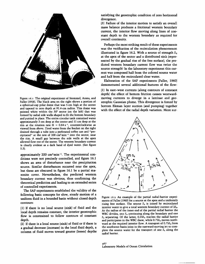
Figure 6.I The original experiment of Stommel, Arons, andFaller 1958). The black area on the right shows a portion ofa spherical-cap polar dome that was 5 cm high at the centerand tapered to zero depth at 91.4-cm radius. This dome waspainted white within the 30° sector on the left) that wasformed by radial side walls shaped to fit the bottom boundaryand puttied in place. The entire circular tank contained waterapproximately 3 cm deep at the center and 11 cm deep at therim at the rotation rate f = 0.84 s-l, counterclockwise asviewed from above. Dyed water from the bucket on the rightdrained through a tube into a perforated coffee can and "pre-cipitated" at the rate of 200 cm3 min-' into the sector, nearthe rim. A small gap between the side walls at the apexallowed flow out of the sector. The western boundary currentis clearly evident as a dark band of dyed water. (See figure5.3).

approximately 200 cm3 min-'. The experimental con-ditions were not precisely controlled, and figure 16.1shows an area of disturbance near the precipitationsource. Similar disturbances occurred near the apex,but these are obscured in figure 16.1 by a partial ma-sonite cover. Nevertheless, the predicted westernboundary current was obvious, thus confirming thetheoretical prediction and leading to an extended seriesof controlled experiments.

The SAF experiments established the validity of thefollowing basic concepts for slow, steady motion of auniform fluid in a bounded basin without closed depthcontours:

(1) If there is no local source (sink) of fluid and thelocal depth remains constant, the interior geostrophicflow is constrained to follow contours of constantdepth.(2) If there is a local source (sink) of fluid or if there isa gradual decrease (increase) in the local fluid depth, acolumn of fluid moves toward greater (lesser) depths

satisfying the geostrophic condition of zero horizontaldivergence.(3) Failure of the interior motion to satisfy an overallmass balance produces a frictional western boundarycurrent, the interior flow moving along lines of con-stant depth to the western boundary as required foroverall continuity.

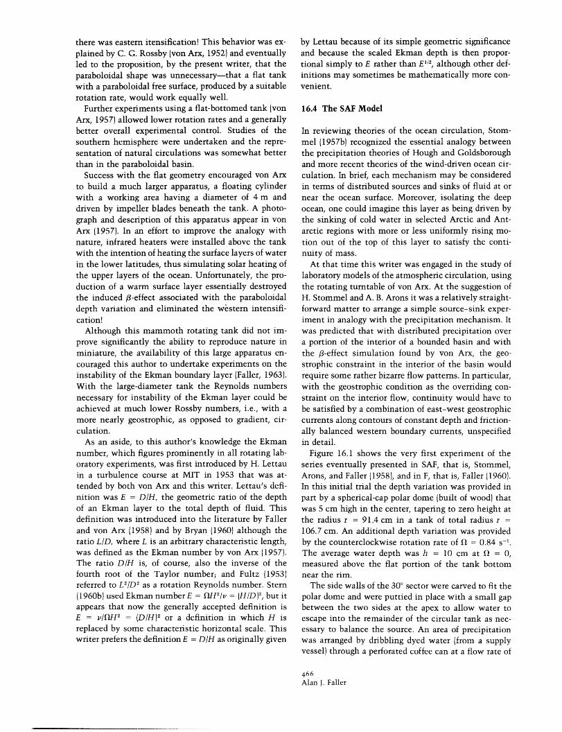
Perhaps the most striking result of these experimentswas the verification of the recirculation phenomenonillustrated in figure 16.2. With a source of strength Soat the apex of the sector and a distributed sink (repre-sented by the gradual rise of the free surface), the pre-dicted western boundary current flow was twice thesource strength! In the laboratory experiment this cur-rent was composed half from the colored source waterand half from the recirculated clear water.

Elaboration of the SAF experiments (Faller, 1960)demonstrated several additional features of the flow:

(1) In east-west currents (along contours of constantdepth) the effect of bottom friction causes westward-moving currents to diverge in a laminar and geo-strophic Gaussian plume. This divergence is forced bybottom Ekman layer suction and pumping) togetherwith the effect of the radial depth variation. More sur-

Figure 6.2 An example of the partial radial-barrier experi-ments of Faller (1960) for a source at the apex and a uniformlyrising free surface. The source So is joined by recirculatedinterior water to give a total western boundary current of 2So.At the radius of the inner end of the partial radial barrier theWBC divides, one So continuing along the boundary and oneSo separating. Of the latter, 0.25So reaches the radial barrierand participates in the WBC there, while 0.75So moves north-ward as the required interior flow. A transport of 0.75So fromthe southwest basin joins in the eastward-moving jet to com-plete the source water for the transport of one So along theradial barrier.

467Laboratory Models of Ocean Circulation

prisingly, the theory, being linear and reversible, pre-dicts that an eastward-moving current of constant massflux should converge into a narrower and more intensejet. As shown in the experiments, catastrophy isavoided in the converging jet because the flow spreadsout in the western boundary current to whatever extentis necessary for its eventual convergence as it flowseastward.(2) With an interior source (or sink) there was an in-tense recirculation analogous to the effects of the wind-spun vortex described by Munk (1950). The intensityof this recirculation phenomenon was found to be inexcellent agreement with a theoretical analysis.(3) The concepts predicted and verified in SAF wereextended to somewhat more complex geometries in-volving partial radial barriers. An example of such aflow, qualitatively verified by experiment, is shown infigure 16.2, where the indicated transports are the the-oretical predictions. Further application to an Antarc-tic-type geometry illustrated the important role of theradial barriers in allowing the buildup of pressure gra-dients essential to the maintenance of the geostrophicflow.(4) In certain source-sink experiments with closedcontours of constant fluid depth, it is not possible toconstruct purely geostrophic regimes of flow. In suchcases, lacking resolution of the problem by westernboundary currents, the effects of bottom friction dom-inate the flow. Examples of the complex set of spiralflow patterns necessary in order to transport fluid froman interior source to an interior sink illustrated thedominance of frictional effects.(5) One feature that would not stand the test of timewas the observation of an eastern boundary currentwhen the flow was injected through the eastern bound-ary of the sector. In later experiments (Faller and Porter,1976) it was found that this current was probably adensity-driven flow due to incomplete thermal controlof the injected water.

The analogy between these laboratory experimentsand theoretical models of steady wind-driven oceancirculation may be illustrated most clearly by a com-parison of the governing equations from three studies.These equations are

Stommel (1948)

Munk (1950)

Faller (1960)

a + V 2 = y sin iry/b,

l eV - A V4q%' = curlZ7,ax

Oh (10/a) Dor r 2

ahat '

In (16.1) a = (H*IR)(af/y), where H* is a cor

and y = Fr/(Rb), where F is the magnitude of themaximum wind stress per unit mass and b the north-south dimension of the model. In (16.2) A is a horizon-tal Austausch coefficient, the wind stress per unitmass, and Ji' the mass transport stream function. In(16.3) h is the variable fluid depth and Q an internal orsurface source of fluid per unit horizontal area.

To illustrate the close correspondence of these equa-tions we may multiply (16.1) by R/H* and convert theright-hand side to the derivative of a cosine; introduce

= '/H as the velocity streamfunction in (16.2), Hbeing the ocean depth; and multiply (16.3) by f/h, re-orient the coordinate axes with rdO = dx and dy =-dr, and add the horizontal viscous term. The threeequations then become

of oaq

ay ax+ V 2+H*

ax' 3x

_1 OF cos ry/bH* Oy

(16.4)

1- A V4t, = curlT,H

( ) a + V2 -V4t,h Oy Ox 2h

(16.5)

f f Q +ah

(16.6)

Equations (16.4)-(16.6) clearly demonstrate the anal-ogy between the laboratory experiment and the basictheories of the steady wind-driven ocean circulation.In particular, (3 = Oflay is modeled by -fh- 1ah/y,Stommel's linear drag law corresponds to the Ekmanlayer effect with R/H* the equivalent of fD/2h, and apositive curl of the wind stress in (16.4) or (16.5) isrepresented in (16.6) by either an internal (or surface)sink of fluid -fQ /h or by a local rate of increase ofdepth (fh) Oahlat. Note also that with the addition ofthe lateral viscous term to (16.6) this equation is ca-pable of describing steady, linear western boundarycurrents analogous to those of Munk.

16.5 Experiments with Rotating Covers

A. 11 aLLLL A.-aJL1- FY LL11-LA I'.. LJAL ALL

than the wind-driven experiments, and the regularboundary conditions of the 600 sector allowed a cleardistinction between the interior flow and the western

(16.2) boundary current (WBCI; turbulence was essentiallyeliminated and the interior flow could be guaranteedto be essentially geostrophic by controlling the flowrates. The introduction of a rotating cover (rotating lid)as the driving mechanism produced a certain degree ofadditional control by completely enclosing the fluid,

nstant by eliminating the possibility of density differences in

effective ocean depth and R a linear drag coefficient;

468Alan J. Faller

the source flow, and by allowing the parameters of theproblem to be more easily varied. For example, tran-sient circulations due to an impulsive start of the coveror due to a periodic oscillation of the cover could beeasily controlled. Such experiments would be difficultwith the sources and sinks of the SAF studies.

Bryan (1960) was perhaps the first to use a rotatinglid in an experiment directed toward the understandingof oceanic circulations. Having in mind the planetarywaves of the atmosphere and the Gulf Stream mean-ders, he investigated the baroclinic stability of a two-layer system of salt and fresh water in a 34-cm-diam-eter cylindrical vessel, the driving force being a slowlyrotating lid. He successfully produced symmetric flow,one to three regular waves, and an irregular wave re-gime, more or less in agreement with a correspondingtheory of baroclinic instability. These experiments, ofcourse, had a great deal in common with the annulusexperiments of Hide (1958) and with the annulus, opendishpan, and two-fluid experiments of Fultz (1953).

Rotating-lid experiments that turned out to be anal-ogous in many ways to the SAF studies were intro-duced by Beardsley (1969) in connection with the the-ories of Pedlosky and Greenspan (1967), the so-calledsliced-cylinder model of the wind-driven ocean circu-lation. The steady-state sliced-cylinder circulation canbe described and understood by a relatively simple the-oretical analysis, and the following section, throughequation (16.18), develops the theory of this model interms borrowed from the theory of the SAF experi-ments. This short section will be of particular interestto those directly concerned with the theory of suchexperiments but may be passed over by the more casualreader. In either case figures 16.3 and 16.4 illustratethe model geometry and circulation.

The radial transport per unit of circumference in theupper Ekman layer due to a differential rotation E issimply TEk(r) = ErDrD/2, and the corresponding sourcestrength per unit area for the interior due to Ekmanlayer divergence is Q = -Ed, independent of radius.For positive E this source is the equivalent of a uniformrise of the free surface in the SAF studies.

At the rim, r = a, the Ekman transport TEk(a) feedsinto a Stewartson boundary layer at the circular wall.Since the interior flow is quite slow for large a, littleof the flow into the Stewartson layer from above canbe taken up by the slow bottom Ekman layer, and weignore this effect. The Stewartson layer then feeds uni-formly into the interior, giving an average flow normalto the wall:

Un = EfaD/2h. (16.7)

U-m- tNIVIAIN LATLK

u\\buU\\I\ '\c'l.\

N I

h=h-y tanca

\ <I aSTEWARTSON

BOUNDARY LAYER LOWER

) 31-\ Q IQII

- Q

Un I

INTERIOR _- C

Vi - -""I

-v - I- I4 -l

EKMAN LAYER

S

Y

Figure 6.3 A schematic N-S cross section of the circulationin a sliced-cylinder model. The circulation is driven by thedivergent Ekman layer of the rotating lid with the inducedsuction velocity Q = -EfID. The Ekman flow at the rim ofthe rotating lid turns into the Stewartson layer and feeds theinterior as a velocity component normal to the wall Un. Thegeostrophic S-N interior flow vi is independent of x and y andis given by vi = -Q/tan a. Global continuity of mass is sat-isfied by geostrophic east-west interior flows and the westernboundary current (not shown).

yI

x

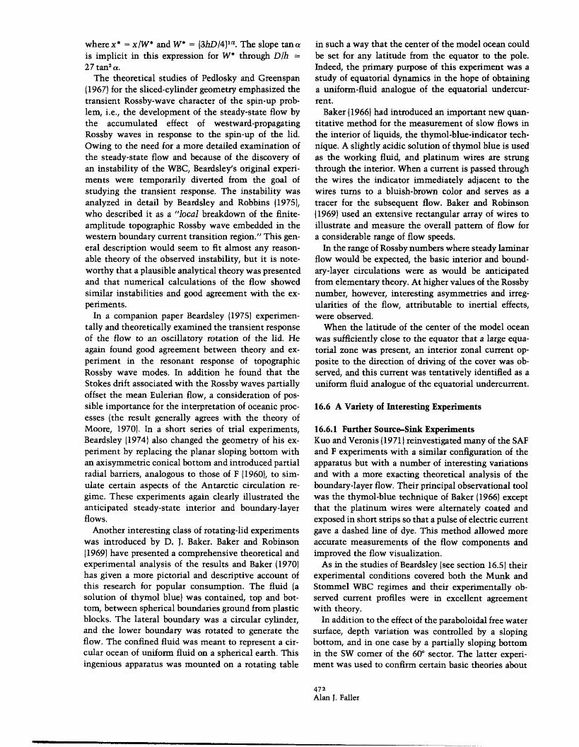
Figure I 6.4 Streamlines of the theoretical, linear, steady-statecirculation in the sliced-cylinder experiment of Pedlosky andGreenspan (1967) and Beardsley (1969) for a bottbm slopeangle a = 30°. For large a the flow away from the easternboundary becomes evident in the streamline pattern becauseof the reduction of vi in comparison to U, (figure 16.3). Thevariation in width of the western boundary current is sche-matically illustrated.

The interior geostrophic flow is governed by equa-tion (16.6) omitting the lateral and bottom friction

469Laboratory Models of Ocean Circulation

1_��������1�1����\\·\�\\\�\,Nxx, N 7XNN

I rlr- /ANI I A\Jr-

1

terms. The resultant equation for the south-to-northinterior flow is

vi = -Q/tana = eD/tana, (16.8)

where v, = OJl/Ox and tana = -Oh y. Thus for E > 0,as in the case considered by Pedlosky and Greenspan(1967), Q < 0 (Ekman suction) and it follows that vi >0. Later experiments of Beardsley used E < 0.

The interior velocity component ui is determined bycontinuity. For a cell in the interior mass continuityis given by

[vih -(vih + avhy dy) dx

+ [uh - (uh + h dx)] dy + Qdxdy =

Using equation (16.8) and hl/O = 0 it is readilyfound that 0ujOx = 0. Following the assertion made inSAF that there can be no geostrophic flow componentnormal to the eastern boundary, but that unlimitedflow into or out of the western boundary layer is per-mitted, the value of u1 is determined by ue, the west-east flow at the eastern boundary. This in turn is com-posed of two parts: the source flow from the Stewartsonlayer is Ue = -Un/cosO = -EflDa/2hcoso; and fromthe constraint that there be no geostrophic flow normalto the boundary we obtain u,2 = -v tan 0. The totalwest-east interior flow is then

Ui = - (d 2h cos 0 tan a) ( 16.9

Integrating (16.8) and (16.9) to obtain an interiorstreamfunction defined by vi = 0t/ax and ui = -P/Oygives

t a sin-'y'-IdDa h 2

+ [(a) 2 tan a a] [1 - (1 -

XI+ x' (16.10)tan a

where y' = y/a, x' = x/a, and q' = 0 at x' = 0, y' = 0.In this integration I have used the approximation

h = h - ytana h (1 E '

and as a result (16.10) differs slightly from Beardsley's(1969) equation for pressure.

Figure 16.4 illustrates the pattern of O' for a = 30°.

With this large slope vi is small and the effect of thesource at the rim is made conspicuous [compare Ped-losky and Greenspan (1967, figure 5)]. Since the rimsource does not directly contribute to the north-south

(N-S) transport, it is easily seen, as pointed out byBeardsley (1969), that the WBC transport Tw is deter-mined solely by the value of vi integrated over x. Bycontinuity

TW(N-S) = - )hvi dx = -2hv, X(yl.-x(Xs)

(16.11)

The WBC transport parallel to the boundary, however,requires that the result in (16.11) be divided by cos 0.Dividing also by eflDah, the nondimensional transportper unit depth and parallel to the boundary is

T(ll) = .2 tan a, (16.12)

the upper sign corresponding to > 0.But although Tw(II) is constant, the current sees dif-

ferent variations of depth Oh/Os along its axis s, and thewidth of the current must change. For positive y andE > 0 as in figure 16.3) the current narrows as it movessouth toward y = 0, and it is also fed from the interiorflow. For y < 0 the current feeds the interior and atthe same time broadens because Oh/Olas decreases alongthe direction of flow. By the time the flow reaches 0 =-7r/2 the WBC must completely disperse, and underthese circumstances it is not surprising that an insta-bility occurs for sufficiently large e.

The steady-state, linear analysis given above cannottake into account transients, instabilities of the flow,details of the boundary layer flow, or the range of va-lidity of the theory. These aspects of the problem werethe principal focal points of the analytic, numerical,and experimental sliced-cylinder studies cited above.Nevertheless, the simplified treatment given here re-veals the essential physical mechanisms withoutmathematical obfuscation. In this spirit we continuewith an elementary treatment of the WBC to illustratecertain principles analyzed by Beardsley (1969) andlater disucssed also by Kuo and Veronis (1971).

Beardsley noted that when the angle a is small, theWBC is dominated by bottom Ekman-layer pumping,rather than by lateral friction. Except very close to thewall, the boundary current then is essentially thatfound by Stommel (1948) with friction entering theproblem through a constant drag coefficient R/H*, asin 116.4).

Figure 16.5 illustrates a WBC profile, the cross-stream Ekman transport beneath the current, and thevertical flux from the Ekman layer. The WBC is nor-mally much wider than D, and in the case where lateralfriction dominates the boundary layer, the ratio of itswidth W' to D is W'ID = (hlD)113(4/tan a)1 3 (see below).Thus, in the Ekman layer the usual boundary-layerassumption applies, namely, that lateral variations ofthe flow can be neglected in comparison to variationsnormal to the boundary. Under the simplifying as-

470Alan J. Faller

ii _

nondimensional coordinate x' = x/W', where W' =[8 hD21(2 tan a)]1'3 will be seen to be the characteristicwidth of the WBC. Then, temporarily neglecting theEkman layer effect by setting D = 0, (16.13) reduces to

d3v- 8v = 0. (16.14)

After applying the boundary conditions the solutionto (16.14) is the exponentially-damped sine profile

v =31 h4W' e- sin /x',(412 hW' (16.15)

which corresponds to the oscillatory solution of Munk11950). A nondimensional v' for this result is plottedin figure 16.5.

The WBC in the absence of lateral friction has beencalled the Stommel boundary layer (Kuo and Veronis,(1971), and from (16.13) this is given by the solution to

dv 2tanadx+ Do. (16.16)

(b) ID 20 30 X'

Figure 6.5 The nondimensional velocity component v' =e-z' sin k for the Munk boundary layer in which lateralfriction dominates the vorticity balance. (b) The Ekman trans-port beneath the boundary layer in (a). (c) Flux into or out ofthe western boundary current by Ekman layer convergence ordivergence. (d) The nondimensional velocity v* = x*e - - atthe transition between the Munk and the Stommel boundarylayer regimes.

sumptions given below it can also be shown that theEkman layer transport is proportional to the local valueof v above the Ekman layer. An inconsistency, apparentin figure 16.5, is that the maximum Ekman layerpumping occurs at x = 0 and the no-slip condition atthe wall is not satisfied. To completely justify the ap-proximate analysis given below, a more completeboundary-layer scaling and analysis including the side-wall Stewartson layers, as given by Beardsley (1969)and Kuo and Veronis (1971), is required.

Here we specify a total northward transport of theWBC, T, a straight N-S boundary, a linear depth var-iation -Oh/Oy = +tan a, and a locally constant depth,where h appears as a coefficient in the final differentialequation; and we neglect variations of the current withy, i.e., along the boundary. Then (16.6) is appropriate,and after dividing by v it reduces to the third-order,ordinary linear differential equation with constantcoefficients

d3v ( h ) dv [ 2 tanav = 0dx3 Dh d D2h

(16.13)

subject to the conditions v = 0 at x' = 0, v = 0 atx' = x, and Tw = fIvh dx. It is convenient to define a

Here the condition v = 0 atx = 0 must be relinquished,and the condition at infinity will be satisfied automat-ically. Applying the transport condition, the solutionis the exponential profile

Th eh W'

where

x" = x/W' and W" = (D(2 tan a).

In terms of a simulated -effect, being given * =(-2fI/h)(ah/Oy) it follows that W" = fIDIh*.

With the scaled coordinate x', the full equation is

d3v dvB - 8v =0,dx'3 dx' (16.17)

where B = 4(D/h )13(2tan a)-2 /3. Substituting the trialsolution v = ekx, the characteristic equation is

k3 + ak + b = O, where a = -B and b = -8

Complex values of k correspond to oscillatory solu-tions, and nonoscillatory boundary layers occur onlyfor (b2/4) + (a3/27) - 0, or D/h - 27 tan2 a. Accordingly,the condition D/h = 27 tan2 a may be defined as thetransition point between the Munk and Stommelboundary layer regimes. In the SAF and F experimentswhere tana = fl2r/g this transition took place at ap-proximately r = 23 cm in a tank of radius a = 100 cm.

The solution at this transition is the product of linearand exponential functions as given by

v= (hW*) x e (16.18)

47ILaboratory Models of Ocean Circulation

V/0.5

04

0.3

Q2

0.1

0

l/

where x* = x/W* and W* = (3hD/4)12. The slope tancais implicit in this expression for W* through DIh =27 tan 2 a.

The theoretical studies of Pedlosky and Greenspan(1967) for the sliced-cylinder geometry emphasized thetransient Rossby-wave character of the spin-up prob-lem, i.e., the development of the steady-state flow bythe accumulated effect of westward-propagatingRossby waves in response to the spin-up of the lid.Owing to the need for a more detailed examination ofthe steady-state flow and because of the discovery ofan instability of the WBC, Beardsley's original experi-ments were temporarily diverted from the goal ofstudying the transient response. The instability wasanalyzed in detail by Beardsley and Robbins (1975),who described it as a "local breakdown of the finite-amplitude topographic Rossby wave embedded in thewestern boundary current transition region." This gen-eral description would seem to fit almost any reason-able theory of the observed instability, but it is note-worthy that a plausible analytical theory was presentedand that numerical calculations of the flow showedsimilar instabilities and good agreement with the ex-periments.

In a companion paper Beardsley (1975) experimen-tally and theoretically examined the transient responseof the flow to an oscillatory rotation of the lid. Heagain found good agreement between theory and ex-periment in the resonant response of topographicRossby wave modes. In addition he found that theStokes drift associated with the Rossby waves partiallyoffset the mean Eulerian flow, a consideration of pos-sible importance for the interpretation of oceanic proc-esses (the result generally agrees with the theory ofMoore, 1970). In a short series of trial experiments,Beardsley (1974) also changed the geometry of his ex-periment by replacing the planar sloping bottom withan axisymmetric conical bottom and introduced partialradial barriers, analogous to those of F (1960), to sim-ulate certain aspects of the Antarctic circulation re-gime. These experiments again clearly illustrated theanticipated steady-state interior and boundary-layerflows.

Another interesting class of rotating-lid experimentswas introduced by D. J. Baker. Baker and Robinson(1969) have presented a comprehensive theoretical andexperimental analysis of the results and Baker (1970)has given a more pictorial and descriptive account ofthis research for popular consumption. The fluid (asolution of thymol blue) was contained, top and bot-tom, between spherical boundaries ground from plasticblocks. The lateral boundary was a circular cylinder,and the lower boundary was rotated to generate theflow. The confined fluid was meant to represent a cir-cular ocean of uniform fluid on a spherical earth. Thisingenious apparatus was mounted on a rotating table

in such a way that the center of the model ocean couldbe set for any latitude from the equator to the pole.Indeed, the primary purpose of this experiment was astudy of equatorial dynamics in the hope of obtaininga uniform-fluid analogue of the equatorial undercur-rent.

Baker (1966) had introduced an important new quan-titative method for the measurement of slow flows inthe interior of liquids, the thymol-blue-indicator tech-nique. A slightly acidic solution of thymol blue is usedas the working fluid, and platinum wires are strungthrough the interior. When a current is passed throughthe wires the indicator immediately adjacent to thewires turns to a bluish-brown color and serves as atracer for the subsequent flow. Baker and Robinson(1969) used an extensive rectangular array of wires toillustrate and measure the overall pattern of flow fora considerable range of flow speeds.

In the range of Rossby numbers where steady laminarflow would be expected, the basic interior and bound-ary-layer circulations were as would be anticipatedfrom elementary theory. At higher values of the Rossbynumber, however, interesting asymmetries and irreg-ularities of the flow, attributable to inertial effects,were observed.

When the latitude of the center of the model oceanwas sufficiently close to the equator that a large equa-torial zone was present, an interior zonal current op-posite to the direction of driving of the cover was ob-served, and this current was tentatively identified as auniform fluid analogue of the equatorial undercurrent.

16.6 A Variety of Interesting Experiments

16.6.1 Further Source-Sink ExperimentsKuo and Veronis (1971) reinvestigated many of the SAFand F experiments with a similar configuration of theapparatus but with a number of interesting variationsand with a more exacting theoretical analysis of theboundary-layer flow. Their principal observational toolwas the thymol-blue technique of Baker (1966) exceptthat the platinum wires were alternately coated andexposed in short strips so that a pulse of electric currentgave a dashed line of dye. This method allowed moreaccurate measurements of the flow components andimproved the flow visualization.

As in the studies of Beardsley (see section 16.5) theirexperimental conditions covered both the Munk andStommel WBC regimes and their experimentally ob-served current profiles were in excellent agreementwith theory.

In addition to the effect of the paraboloidal free watersurface, depth variation was controlled by a slopingbottom, and in one case by a partially sloping bottomin the SW corner of the 60° sector. The latter experi-ment was used to confirm certain basic theories about

472Alan J. Faller

____ __

the effect of bottom topography on the separation ofthe boundary current from the coast. Concentratedsources and sinks in the interior, similar to the sourceused in F (1960) and to the effect of the wind-spunvortex of Munk (1950), also illustrated separation ofthe boundary current because of the source-sink dis-tribution.

Veronis and Yang (1972) extended the uniform fluidWBC theory and experiments to cases with signifi-cantly nonlinear flow. Once again, the theoretical pre-dictions, including both lateral viscous and Ekmanlayer effects, were accurately verified in the experi-ments. Some unsuccessful attempts were made to pro-duce a sufficiently rapid and narrow western boundarycurrent for barotropic instability.

16.6.2 A Two-Layered ModelA major innovation and advance in laboratory model-ing has recently been achieved by Krishnamurti (Krish-namurti and Na, 1978; Krishnamurti, 1978) by the in-troduction of controlled rotating-lid experiments witha two-layer system having no closed contours of depth.Using a conical bottom and a rotating conical lid, radialdepth variations are produced in both the upper andlower layers. Under conditions that would be stable fora uniform-fluid experiment, the two-fluid experimentproduces baroclinic instability and a number of inter-esting features associated with the deformation of theinterface of the two fluids. Perhaps the most strikingof these features is the upwelling of the lower fluid tothe "surface" at the western boundary and the concur-rent separation of the WBC, a phenomenon predictedby Parsons (1969) (see chapter 5).

Together with the laboratory experiments, Krishna-murti (1978) has theoretically evaluated the compara-tive spin-up times of the ocean and laboratory modelsin terms of the Rossby radius of deformation in relationto the fluid depth. These considerations suggest thatthe two-fluid experiments will have a number of in-teresting applications.

16.6.3 Flow over Sills and Weirs and through StraitsSmith (1973, 1977) was concerned with the flow of coldbottom water after it had passed through the DenmarkStrait from the Norwegian Sea. This is a problem con-cerning effects of friction and sloping bottom on themodification of a baroclinic current system. To accom-pany a theoretical model of bottom frictional effects,Smith developed a laboratory experiment in whichdenser fluid was drained slowly through a source tubeonto the sloping bottom of a rotating tank. He observeda variety of systematic wavelike and eddy-like oscil-lations of the flow that were found to be consistentwith appropriate theories of baroclinic instability. Inthe 1977 paper he compared his experimental results

with observations of the pulsed flow over the sill inthe Denmark Strait, and he concluded on the basis ofthe significant nondimensional numbers that the nat-ural case should correspond to what he described as"the meandering jet, vortex train variety (Class I)."Experiments of this type indeed represent a sophisti-cated application of laboratory experiments to our un-derstanding of detailed oceanic phenomena.

Flows through straits and over sills have been ofgreat interest in a wide variety of nonrotating systems,and engineering data characterizing these flows havelong been available. In oceanic applications, however,the Coriolis force must play an important role in mod-ifying or controlling the flow, and from experience withtopographic 3-effects one might also expect the de-tailed geometry to be of great significance in manycases. An obvious oceanographic example of restrictedflow is that through the Straits of Gibraltar, but manyother examples may also be mentioned, such as theseepage of Antarctic Bottom Water through small gapsin the Mid-Atlantic Ridge.

The experiments of Whitehead, Leetmaa, and Knox(1974) and of Sambuco and Whitehead (1976) have beenconcerned with problems of this type, approachingthem experimentally beginning with the nonrotatingsystem and gradually increasing the effect of rotation.Their studies may be characterized as being concernedchiefly with the restriction of the volume transport ofthe lower fluid through the strait, or over the sill, atrelatively high Rossby numbers. Smith's studies, incontrast, have been concerned primarily with very lowRossby numbers, and with frictional effects on slopingboundaries after the flow has left the constriction.

16.6.4 The Generation of Mean Flows by TurbulenceOne of the more elaborate and more significant recentlaboratory studies has been that of Colin de VerdiEre(1977), who examined the response of a rotating fluidin various geometries to Rossby waves generated by acomplex pattern of oscillatory sources and sinks offluid introduced through holes in the bottom of thetank. He considered three cases: an f-plane model (con-stant depth); a polar 3-plane model with a depth vari-ation from the paraboloidal shape of the free surfaceand with closed height contours; and a sliced-cylindermodel. Comparing turbulence and wave theory withthe complex flow patterns of his experiments, he in-cluded in his studies the interaction of two-dimen-sional turbulent eddies for a fluid with energy sourcesand sinks, the evolution of the flow toward statisticalequilibrium, and the interaction of Rossby waves witha mean flow.

The extent and variety of the experiments coveredby Colin de Verdiere preclude a detailed exposition ofall his results, but in general it may be said that thetheoretical expectations, based upon the theories of

473Laboratory Models of Ocean Circulation

potential vorticity mixing of Rhines (1977), were ex-perimentally verified. By way of example, we mentionhere the results of a polar p-plane experiment in whichthe flow was driven by alternating sources and sinksof fluid at the outer boundary. This complex systemwas arranged to produce a westward-moving Rossbywave. Through the preferential inward (northward) dif-fusion of anticyclonic vorticity, the Rossby wave ineffect transferred energy to a westward mean flownorth of its region of generation. When the forcing wasturned off and the flow was allowed to decay, meas-urements of the mean flow and of the perturbationkinetic energy indicated that the eddies continued tofeed energy into the mean flow.

The particular results given above concerning thegeneration of mean flows by turbulence in a -planemodel were anticipated by the experiments of White-head (1975), who excited turbulent motions in a some-what different manner. Whitehead used a 2-m-diametercylindrical tank and vertically oscillated a circular hor-izontal plastic disk within the fluid, the disk being 20cm in diameter and centered at 66 cm radius. By thusdriving turbulence and Rossby waves with no directinput of angular momentum, it was clear that the ob-served mean flow [eastward at the latitude (radius) ofthe oscillator, and westward to the north and south]was due to the lateral redistribution of angular mo-mentum by the waves and turbulence. In such exper-iments, however, it is difficult to be certain that themechanical apparatus is not partially forcing the meanflow. Suppose, for example, that the vertical axis of theoscillating plate were tilted by 1° one way or the other.Would this have an influence upon the generation ofthe mean flow, and if so, how much? The experimentsof Colin de Verdiere, using sources and sinks parallelto the rotating axis, do not seem to be subject to thesame possible difficulties, but one must be very cau-tious in experiments of this type.

It is interesting to note that the late Professor V. P.Starr (of Chicago and MIT) probably had a significantinfluence upon these studies, for Whitehead acknowl-edges many interesting conversations with Starr andhis students. I note this fact particularly because it wasat the suggestions of Professors Starr and Rossby thatFultz began his experimental studies at the Universityof Chicago, and one of the original intentions of thosestudies was an examination of exactly the problemdiscussed above. The experiments of Fultz eventuallycentered upon thermally driven circulations in a hem-ispherical shell, but Starr (personal communication,circa 1952) always kept in mind the possibility of lo-cally pulsing one of the spherical shells to generatepurely mechanically driven circulations without thedirect introduction of a mean flow.

The experiments discussed above appear to be con-tradicted by an experiment of Firing and Beardsley(1976), who generated an isolated eddy in a sliced-cyl-inder experiment. It was found that the total nonlineareffect of the eddy was the generation of cyclonic vor-ticity in the northern portion of the basin and anticy-clonic vorticity to the south. The net effect was ex-plained as the result of the competition between twoopposing tendencies:

Potential vorticity conservation which imparts nega-tive vorticity to northward moving water columns andpositive vorticity to southward moving columns, andrelative vorticity segregation which gives water col-umns with positive relative vorticity a tendency tomove north and those with negative vorticity a ten-dency to move south. Thus the positive circulationinduced in the northern half of the basin by the dis-persing eddy indicated the dominance of the vorticitysegregation mechanism in this flow.

There is need for further theoretical and experimen-tal studies to rationalize the apparent differences be-tween these results and those of Colin de Verdiere(1977) and Whitehead (1975). The experiment of Firingand Beardsley was conducted in a system with noclosed geostrophic contours and with an isolated eddyas the disturbance. The other experiments had contin-uous sources of Rossby waves or turbulence in an opencircular tank without meridional barriers and thereforewithout the possibility of western boundary currentand Rossby-wave reflection from meridional barriers.

16.6.5 The Generation, Propagation, and Reflectionof Rossby WavesTopographically generated Rossby waves were studiedin detail by Long (1951) for the flow between hemi-spherical shells. Since that time many experimentershave generated stationary Rossby-wave patterns by theflow over a ridge or obstacle, using the radial depthvariation to produce the simulated f-effect. StationaryRossby waves have also appeared in a variety of exper-iments where the flow was obliged to separate fromthe western boundary and the boundary current wassufficiently nonlinear.

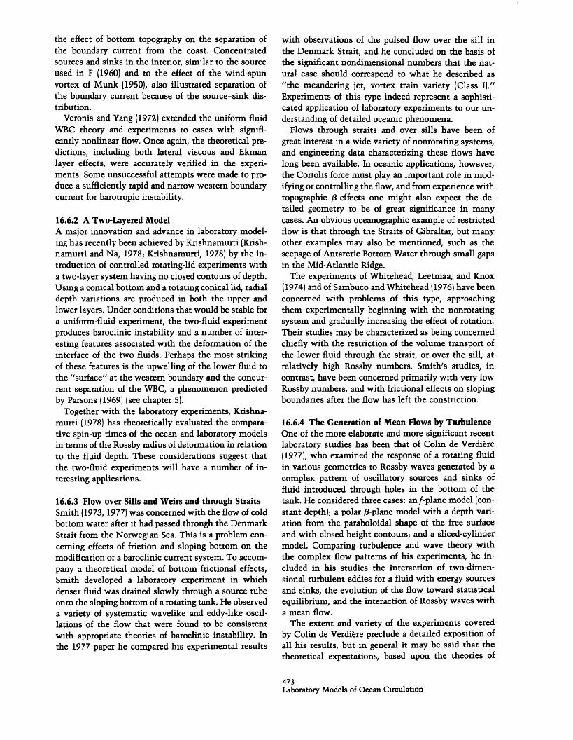
Ibbetson and Phillips (1967), however, were the firstto investigate the generation, propagation, and reflec-tion of Rossby waves specifically in an oceanographiccontext. In their classic paper they experimentallystudied the free propagation and dissipation of Rossbywaves from an oscillating-paddle wave generator (figure16.6). Moreover, they developed a simple theory and acompanion experiment for damped oscillatory flow inthe closed region between their oscillating paddle anda radial barrier to the west. For a specific paddle fre-quency their theoretical solution consisted of the sumof two waves of the same frequency that could beidentified as the one generated in the east by the paddle

474Alan J. Faller

_� I_ __ I_ __ _ _ __ ___

Figure 6.6 A schematic representation of the Ibbetson andPhillips (1967) experiment for the limiting case of zero fre-quency of the oscillator. The interior currents are then purelyzonal with speeds v, equal to the speed of the eastern boundaryUe. The steady-state western boundary current transport isdetermined by continuity as in the SAF (1958) experiments.

and its reflection from the western boundary. Since thereflected wave was of high wavenumber and large am-plitude, its energy was subject to rapid dissipation asit progressed eastward from the boundary. The net re-sult was a strong concentration of radial motions inthe vicinity of the western boundary.

The application of these results to steady-stateocean-circulation theory, as well as to the transientoscillations, becomes evident when one lets the drivingfrequency of the paddle approach zero. This conditionis illustrated in figure 16.6. From section 16.5, becausethere are no interior sources and sinks of fluid, theinterior radial velocity is v = 0. It also follows thatui = ue, where ue is the zonal velocity of the easternboundary, which in this case is the velocity of thepaddle. The wave generated by the paddle thus degen-erates to purely east-west currents, and the reflectedwave, with very high longitudinal wavenumber andvery large radial flow, in the limit becomes the westernboundary current.

16.6.6 Simulation of the American MediterraneanAn account of laboratory models of ocean circulationwould not be complete without a brief discussion ofIchiye's (1972) laboratory studies of flow in the Gulf ofMexico and the Caribbean Sea. These were attempts toreproduce the known circulations insofar as is possiblewith a uniform fluid, by detailed scaling of the complexcoastlines and bottom topography. The avowed pur-pose was "to understand the effects of bottom andcoastal configuration of the two seas on the geostrophiccurrent of barotropic mode. The vertical structure ofthe flow and the details of the horizontal current pat-terns are not a subject of this study."

Two separate model systems were constructed: onefor the Gulf of Mexico, driven by a source of forcedinflow through the Yucatan Straits, and outflowthrough the Straits of Florida; the other, of the Carib-

bean Sea and adjacent portions of the Gulf and theAtlantic Ocean, driven by a pattern of winds from fans.Rossby numbers and Reynolds numbers of the flowwere varied to discover how the overall patterns offlow and the various cyclonic and anticyclonic vorticeswould respond to different values of these parameters.

In summary it may be said that many realistic fea-tures of the natural circulations were reasonably wellreproduced, for example, the distribution of geo-strophic mass transport in the Caribbean; but other fea-tures, notably the major current systems in the Gulf,were unacceptable. Of course, one of the values ofexperiments of this type lies in failure, for we are thendirected to inquire about the specific sources of error.In this study it is likely that density stratification, orat least a two-layer system, may be necessary forgreater realism of the model circulations. With thestrong topographic effects that must be important inthese nearly enclosed basins, the normal -effect maybe negligible, and a stratified-fluid experiment may bepractical.

16.6.7 A Laboratory Study of Open-Ocean BarotropicResponseThe above title is that of Brink (1978), who studiedthe f-plane and r-plane response of a rotating fluid witha free surface to applied surface-pressure oscillations.A problem of direct interest is the response of the worldoceans to atmospheric pressure fluctuations of allscales (see chapter 11). In the absence of the planetaryand topographic -effects, the f-plane response shouldfollow the inverse barometric effect except for frequen-cies close to resonance with inertia-gravity waves.When near resonance occurs there may be significantovershoot, i.e., excess amplitude response compared tothe inverse barometer effect. With the 8-effect therecan be significant undershoot because of the propaga-tion of Rossby waves, although if the scale and fre-quency of the pressure fluctuations should correspondto one of the normal modes of oscillation of the basin,there again could be significant overshoot.

In his -plane experiments, Brink oscillated the airpressure over an enclosed region bounded by circulararcs at 15.2- and 30.5-cm radius and by radial wallsseparated by 1200 of azimuth. With the tank radius of42 cm, the area of forced-pressure oscillation comprisedabout 13% of the total surface area. The pressure vesselwas designed to just touch the water surface with theintent of not seriously interfering with the water cir-culation or the propagation of waves. Measurements ofthe water-level response were obtained with capaci-tance height gauges.

Approximate theoretical solutions for the responseof the water level were compared with the amplitudesand phases of the observed height variations at several

475Laboratory Models of Ocean Circulation

sites. Reasonable agreement was found in many cases.The most serious lack of agreement occurred at thehigher frequencies, and this was tentatively attributedto the use of a primitive (steady-state) Ekman-layermodel for viscous damping, rather than one that tookinto account transients in the Ekman layer. Brink con-cluded that departures from the inverse barometer ef-fect are to be expected due to propagating free modesof oscillation as predicted by theory.

16.6.8 Gulf Stream RingsA laboratory study that may have direct analogy to theocean was that of Saunders (1973), who experimentallytested the stability of a two-layer baroclinic vortex.While this experiment was similar in certain respectsto the baroclinic instability studies of Fultz (1953),Hide (1958), Bryan (1960), Hart (1972), and others,Saunders pursued an interesting analogy with the sta-bility of Gulf Stream Rings and other isolated oceanicvortices.

A cylindrical column of denser fluid was releasedwithin a lighter fluid, the entire system being initiallyin solid-body rotation. The lower part of the denserfluid spread out rapidly, leading to a low-level anticy-clonic vortex and an upper-level cyclonic vortex. Theincrease in radius at the bottom R - R0 from the initialradius of the cylindrical column R0 was approximatelyequal to X = (g'H)112/f, the Rossby radius of deformation,where g' = g Ap/p, Ap is the difference in fluid densities,H the fluid depth, and f the Coriolis parameter.

Defining the parameter 0 = X2/R2, it was found thatfor 0 < 1 the initial circular vortex was unstable andwould break up into a number of smaller vortices, eachhaving 0 > 1.

Calculation of an equivalent value of 0 for two stableGulf Stream rings gave 8 = 2. Thus the stability orinstability of the laboratory vortices and the corre-sponding stability characteristics of Gulf Stream rings,or other nearly circular oceanic vortices, may representone of the most unambiguous tests of baroclinic insta-bility in the ocean.

Two items that may be of historical interest in con-nection with these experiments are the following. First,in studies designed to test the bubble theory of cu-mulus convection Saunders used a small, hemispheri-cal volume of buoyant fluid released at the bottom ofa large and deep tank of water. Turned upside down, asmall volume of dense fluid was released and allowedto fall, expanding as an entraining spherical-cap bubble.Saunders noticed that when the falling dense fluid im-pinged upon a rigid boundary it spread out somewhatanalogously to an atmospheric squall line, and a seriesof experiments in a shallow fluid were undertaken.Since von Arx's old rotating turntable was available inthe same laboratory, extension of these experiments to

the rotating system was quite practical without theconstruction of new elaborate apparatus. Saunders firstperformed these rotating experiments in 1963 and thecritical parameter for the stability of this type of vortexin fact was determined well before the extent and sig-nificance of Gulf Stream rings were fully appreciated.

The second item of interest is that in the late sum-mer of 1954, when this author was first using von Arx'sapparatus for atmospheric model studies, H. Stommeland W. V. R. Malkus one day suddenly appeared in thelaboratory equipped with huge jugs of xylene and car-bon tetrachloride (which at that time were not knownto be so dangerous). Their intention was almost exactlythe experiment later performed by Saunders, namely,to release a cylindrical column of a dense mixture oftheir two fluids in the center of a rotating tank full ofwater. They were specifically interested in relating theradial spread of this column of dense fluid to theRossby radius of deformation, which had recently beenrecognized as an important parameter. Unfortunatelythis combination of liquids would have dissolved thesealer cementing together the base and rim of the tank.How might the history of laboratory studies have beenaltered in its course had this author allowed them toproceed with their experiment?

16.6.9 Spin-UpLaboratory experiments and the theory of spin-up of arotating fluid began with the work of Stern (1959,1960b). In the former (unpublished) paper he presentedthe basic theory of spin-up and a description of labo-ratory experiments that accurately verified the pre-dicted spin-up times as well as the integrated radialand tangential displacements of floating tracer parti-cles. In the latter paper an instability of Ekman flowwas postulated as the source of disagreement betweenthe experiments and laminar theory in certain cases.In more recent experiments, also with a uniform fluid,Fowlis and Martin (1975) used a laser Doppler veloci-meter and found clear evidence of the elastoid-inertiaoscillations to be expected from transients in the Ek-man layer owing to the abrupt change in rotation rate(Greenspan and Howard, 1963). In the wind-drivenocean, however, the stratification may drastically alterthe spin-up characteristics from what would be antic-ipated for a uniform fluid.

Stratified spin-up experiments (e.g., Buzyna and Ve-ronis, 1971; Saunders and Beardsley, 1975) generallyhave been conducted in the same manner as the clas-sical uniform fluid cases-with an abrupt change inthe rotation rate. In such a case, all natural modes ofoscillation can be excited, and as a result it has beendifficult to match satisfactorily theory and experiment.In recent studies by Beardsley, Saunders, Warn-Varnas,and Harding (1979), however, the spin-up was made

476Alan J. Faller

�__ ___ __t__ _ _I I I

gradually, thus avoiding the excitation of high-fre-quency oscillations. As a result, substantially betteragreement than in previous experiments was foundbetween a simple quasi-geostrophic numerical modeland observations of the response of the interior tem-peratures and the azimuthal velocities.

16.6.10 Langmuir CirculationsOne of the areas of research in which H. Stommelplayed an early role was the study of windrows-slickson a natural water surface oriented in streaks along thewind direction. In a series of approximately 200 obser-vations on Ashumet Pond, Cape Cod, Massachusetts,over the 7-month period May-November 1950, Stom-mel (1952) observed the presence or absence of surfacestreakiness parallel to the wind, and he attempted torelate the occurrence of streaks to various meteorolog-ical factors including the wind, cloudiness, humidity,and the air-water temperature difference as a measureof the thermal stability. The single parameter thatseemed to be related to the occurrence of streaks wasthe wind speed, and table 16.1 is a summary of Stom-mel's data. The occurrence of streaks is clearly seen tobe dependent upon the wind speed, and streaks oftenwere observed at speeds much less than what is nowgenerally considered to be the critical value, about3 m s- (Walther, 1966).

These data do not seem to indicate a sharply definedcritical speed, and the apparent critical speed given byother observers should perhaps be questioned in viewof the facts that the observation of streakiness is asubjective one, the amount of surface material presentmay be a factor, and parameters such as the steadinessof the wind measured just above the water surface maybe relevant.

Because of the obvious presence of surface films andbecause "if the wind changes its direction abruptly thestreaks themselves are quickly reoriented (in a matterof one or two minutes only)," Stommel (1952) postu-lated that the phenomenon was essentially a shallowsurface-layer effect and that the action of the film indamping capillary waves might be of importance for

Table 16.1

Number of observations

Wind speed (mph) Streaks No streaks % streaks

<1.5 3 42 71.5-2.5 9 19 32

2.5-3.5 11 8 58

3.5-4.5 14 5 74

4.5-5.5 13 8 62

>5.5 54 3 95

organizing the film into streaks. This postulate wastaken up and explored by other authors, but it is nowknown that the windrows are the result of Langmuircirculations (LCs), organized longitudinal rolls withtheir axes parallel to the wind, and that surface filmsare not an integral part of the mechanism.

Since several scales of LCs may exist at any time(Faller and Caponi, 1978) the apparent rapid responseof the windrows to wind variations may be presumedto be due primarily to the smaller scales, which areclose to the surface and which respond more rapidly tochanges in the wind. For example, in recent laboratoryexperiments with light wind Faller (1978) has found acharacteristic growth rate of only 12 s for cells with across-wind wavelength of 44 cm. For larger scales onewould certainly expect slower response times, but itnow appears that reorganization of the pattern of sur-face streaks in a minute or two by the reformation ofthe LCs is not unreasonable.

I would now like to report some preliminary quali-tative results on the generation of LCs in the presenceof surface films. Figure 16.7 illustrates the wind-wavetank in which a regular pattern of crossed waves isgenerated and in which a wind is blown over the waves.In the absence of a finite-amplitude crossed-wave pat-tern and at low wind speeds there are virtually no windwaves generated over the working section of the tank,a length of about 5 m. In the presence of finite-ampli-tude crossed waves, however, the same air speed causeswind-generated waves of significant amplitude. Frompreliminary estimates it now appears that the largecrossed waves and the smaller wind-generated wavesboth contribute to the growth of the observed LCswhose scale is determined by the crossed-wave pattern.

In previous papers (Faller, 1969; Faller and Caponi,1978), it was reported that surface films completelyprevented the formation of LCs, but this assertion mustnow be qualified on the basis of recent experiments. Ofparticular importance here is the effect of the finitelength of the wind-wave tank, for this restricts thepossible motion of the film. In light-wind conditionsthe wind stress will compress the surface film againstthe end of the tank, and a steady state is achieved whenthe internal film-pressure effect balances the windstress. This condition can be avoided, at least tempo-rarily, by introducing a surface film onto a clean watersurface at the upwind end of the tank, for the film canthen move downwind in response to the wind stress.

The effects of surface films under certain laboratoryconditions can now be summarized as follows:

(1) Application of a surface film-forming material, inthis case dodedyl alcohol, always damps wind-gener-ated waves. Thus, whether moving or stationary, a filmalways destroys the contribution of small wind-gener-ated waves to the LCs.

477Laboratory Models of Ocean Circulation

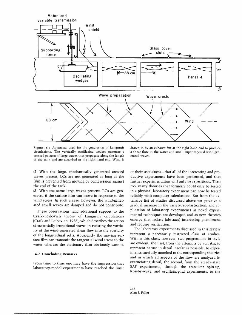
Motor andvariable transmission

Windshield

Support ngframe

Glass coverslots

II -

-I' S

Oscillating Panel 4wedges

Wave propagation

Figure 6.7 Apparatus used for the generation of Langmuircirculations. The vertically oscillating wedges generate acrossed pattern of large waves that propagate along the lengthof the tank and are absorbed at the right-hand end. Wind is

(2) With the large, mechanically generated crossedwaves present, LCs are not generated as long as thefilm is prevented from moving by compression againstthe end of the tank.(3) With the same large waves present, LCs are gen-erated if the surface film can move in response to thewind stress. In such a case, however, the wind-gener-ated small waves are damped and do not contribute.

These observations lend additional support to theCraik-Leibovich theory of Langmuir circulations(Craik and Leibovich, 1976), which describes the actionof essentially irrotational waves in twisting the vortic-ity of the wind-generated shear flow into the vorticityof the longitudinal rolls. Apparently the moving sur-face film can transmit the tangential wind stress to thewater whereas the stationary film obviously cannot.

16.7 Concluding Remarks

From time to time one may have the impression thatlaboratory-model experiments have reached the limit

Wave crests

drawn in by an exhaust fan at the right-hand end to producea shear flow in the water and small superimposed wind-gen-erated waves.

of their usefulness-that all of the interesting and pro-ductive experiments have been performed, and thatfurther experimentation will only be repetitious. Thentoo, many theories that formerly could only be testedin a physical-laboratory experiment can now be testedreliably with computer calculations. But from the ex-tensive list of studies discussed above we perceive agradual increase in the variety, sophistication, and ap-plication of laboratory experiments as novel experi-mental techniques are developed and as new theoriesemerge that isolate (abstract) interesting phenomenaand require verification.

The laboratory experiments discussed in this reviewrepresent a necessarily restricted class of studies.Within this class, however, two progressions in styleare evident: the first, from the attempts by von Arx torepresent nature in detail insofar as possible, to exper-iments carefully matched to the corresponding theoriesand in which all aspects of the flow are analyzed inexcruciating detail; the second, from the steady-stateSAF experiments, through the transient spin-up,Rossby-wave, and oscillating-lid experiments, to the

478Alan J. Faller

"-II--- --- -- ---

interaction of turbulence and the mean flow. The re-cent two-fluid experiments of Smith, Saunders, White-head, and Krishnamurti now seem to indicate a gradualprogression from uniform-fluid models into the theo-retically and technically more difficult realm of baro-clinic models, and clearly it would be premature toconclude that there is no longer a role for laboratorystudies. Indeed, as long as "no one believes a theory,except the theorist, and everyone believes an experi-ment-except the experimenter," the role of laboratoryexperiments in oceanographic research remains secure.

479Laboratory Models of Ocean Circulation