Of Flower Blooms and Female Booms:

The Impact of The Flower Industry on Female Outcomes

Sara Hernández⇤

August 15, 2015

Abstract

This paper investigates the impact the growth of the fresh-cut flower industry had on the lives of

Colombian women. My goal is to understand how flower shocks affect the timing of fertility and marriage

decisions for women exposed to them during their adolescence. The empirical strategy exploits municipal

variation in the geo-climatic suitability for floriculture together with time variation from the industry’s

growth. I find that girls exposed to the flower shocks are more likely to have initiated sexual activity, to be

pregnant and married at younger ages. The results remain robust to different forms of shock aggregation,

differential trends by municipality characteristics, accounting for migration, and geographically restricting

the sample to the departments that concentrate flower production.

Keywords: Flower Exports, Colombia, Fertility, Marriage, Sexual Initiation

⇤I am extremely grateful to Esther Duflo her feedback and guidance. Special thanks to Frank Schilbach for all his commentsand suggestions. Joel Yuen and Raissa Fábregas were avid proofreaders. Ana Bermúdez and Jorge Bermúdez provided expertinsights into the Colombian flower industry. All errors are my own. PhD Candidate. Massachusetts Institute of Technology,Department of Economics. Email: sara_hdz@mit.edu

1

1 Introduction

The feminization of the labor force has been a shared phenomenon across many emerging economies. The

incorporation of females into the labor market has often relied on the expansion of the manufacturing and

agro-processing industries, spurred by international trade. Leading examples of this experience are found

in the textile and garment industries of Bangladesh, the maquilas of México and the dagongmei in China.

In the present context of growing global trade, the question of whether and how fertility timing outcomes

respond to local employment shocks is of primary relevance for development economists.

This paper exploits the dramatic growth in the Colombian flower industry to evaluate the impact em-

ployment opportunities have on an array of events relating to the lives of Colombian women. The outcomes

that I concentrate on are: initiation of sexual activity, first pregnancy and marriage. As mentioned, the

labor shocks come from the Colombian flower industry, which emerged in the year 1965. The arrival of these

flower jobs soon transformed the landscape of formal employment opportunities, particularly for women,

offering them ‘wages, security, and [a] sense of community’ (Friedeman-Sánchez, 2006). It is also throughout

this period that Colombia experienced a secular increase in the female labor force participation rate, going

from 47 percent in the 1980s to 65 percent by 2006 (Amador et al, 2012).

For this study, I use several waves of the Demographic and Health Surveys (DHS) from 1986, 1990, 1995,

2000, 2005 and 2010. This allows me to construct a repeated cross-sectional sample of females born between

1952 and 1997. I then link their fertility and marriage outcomes with the municipality-level flower conditions

while they were growing up.

Understanding the factors that affect whether a female will be sexually active, pregnant or married during

her adolescence remains a pressing issue. Worldwide, about 16 million girls aged 15 to 19 give birth every year,

and close to 1 million do so under 15 (WHO, 2014). The risks and consequences of adolescent pregnancies

are acute: not only for the health of both infant and mother, but also for what they entail in economic

terms. Females who begin motherhood at earlier ages “pay the highest wage penalty for childbearing” (ibid),

and girls who marry in their adolescence are likely to enter into adulthood in extremely unequal conditions

(UNFPA, 2013). Postponing their first birth allows young women to continue investing in their education,

work more and live independently later in life (Miller, 2005).

At the global level, the prevalence of pregnancies among girls less than 18 years of age has seen a slight

decline over the past decades. Singularly, Latin America and the Caribbean have been the exception to that

trend (UNFPA, 2013). In Colombia, there is evidence that the adolescent pregnancies are more likely to occur

among the poor and uneducated (DHS, 2010). Thus, I hypothesize that the exposure to local employment

shocks might affect the lives and choices of these young women, ultimately altering their exercise of agency.

2

In my setting, the exposure to the rose jobs will depend simultaneously on the interaction between two

sources of variation: (i) being an adolescent in a municipality that is a flower producing center and (ii) the

international market conditions for the flower exports. To address endogeneity concerns about the location

of flower farms, I proceed with an instrumentation strategy that depends on geo-climatic conditions. This

allows me to determine the suitability of a municipality to become a flower-producing center. With the aim

to generate shocks to the value of flower exports, I incorporate the Colombian peso exchange rate into the

2SLS strategy.

In summary, I find that a 10% increase in the flower value results in a significant increase of 1.037

percentage points (pp) in the probability of sexual initiation by age 17 in flower suitable municipalities.

In relative terms, this corresponds to a 2.16% more above the mean fraction of females who were sexually

active by that age over the sample period—48.1% of them. The significant increase in the initiation of sexual

activity is also found to be aligned with a positive impact on early childbearing. In particular, the 10%

rise in the flower value leads to a differential increase of 0.598 percentage points in the probability of being

pregnant for the first time by age 17. Considering that 21.5 percent of the females had been pregnant by that

age, that corresponds to a 2.78% increase over the sample period. Their marriage1 decision is also positively

and significantly affected. The impact remains positive when the events are evaluated at the younger age of

15, albeit the pregnancy event becomes marginally significant.

My results remain robust to different forms of shock aggregation: I analyze export value changes that

occur on a particular year, and also shocks that are aggregated across time, thus representing a finer form

of total exposure to the industry. I also control for differential trends by municipality characteristics and

regional, linear time trends. I show that the estimates are also consistent for the sample of females for

whom I know their migration history. By tracking the municipalities in which they grew up, I can better

determine the actual exposure to the flower industry. As a further check, I contrast the flower shocks on the

sample of women who were migrants (and for whom the municipality of residence during their adolescence

is unknown), and I find no significant impact. Last, I restrict my analysis to the two Departments2 that

concentrate flower production and the findings remain consistent.

The results emanating from the rose jobs offer a subtle picture on the impact that the expansion of

export-oriented semi-industrial employment opportunities has had for women in the developing world. By

examining how the timing of sexual initiation, childbearing and nuptiality change across cohorts in response

to differential employment shocks, I provide new evidence of how the transition into marriage and first

birth is being shaped by international trade forces. Remarkably, these modern factory-line type of jobs, the

1The definition for the marriage category includes any type of union: legal marriage and cohabitation.2Departments in Colombia are autonomous country subdivisions. There are 32 departments, and each of them agglomerates

multiple municipalities.

3

epitome of today’s globalization, accelerated the timing of early sexual and reproductive events for females.

The remainder of the paper is organized as follows. In Section II, I describe the institutional context and

the development of the flower industry in Colombia. In Section III, I provide an overview of the identification

strategy. In Section IV, I describe the data, and Section V is devoted to presenting the estimation results.

Finally, Section VI concludes.

2 Institutional Context

2.1 Fertility and Marriage Evolution in Colombia

Colombia is an Andean republic whose political stability in the last century was ghastly eroded by factional

internal dissent. Its modern history has been characterized by political strife, arising from a three-way

conflict between: the two leftist guerrilla groups, the Fuerzas Revolucionarias de Colombia (FARC, in its

Spanish acronym) and Ejército de Liberación Nacional (ELN); the military, representing the government;

and paramilitary groups.

Despite this geography of terror, Colombia saw profound transformations and steady economic devel-

opment in the last half century: rapid urbanization, mass education and a rural exodus, amidst the major

ones (Rosero-Bixby et al, 2009). Amador et al (2012) add the dramatic change in female participation as

another force reshaping the Colombian economic landscape. In their findings, it is worth mentioning that

the groups that exhibited the highest increases in participation are women with children younger than 18,

married women, and women with low educational attainment.

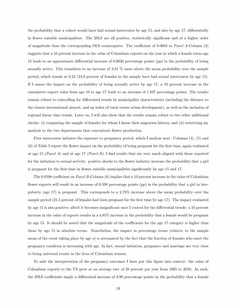
For this study, the nature of the outcomes of interest relates to the timing of sexual initiation, first

pregnancy and first union. I begin with a graphical representation of these trends in Figure 1. First, in

Figure 1a, I look at the fraction of females who have been sexually active and pregnant by age 15, separately.

The sexual initiation and the first birth probabilities, as of age 15, remained remarkably stable from the early

1950s into the late 1960s, and saw a gradual increase thereafter. In the same graph, I also identify 1952,

since females born this year will reach their fertile age (age 13) in 1965, which marks the first Colombian

shipment of fresh-cut roses to the US. Thus, cohorts born after 1952 came into a world where roses offered

a promising source of employment. Second, in Figure 1b, I graph the average number of children and the

average age for sexual initiation by birth cohort.3 The tendency in these two events is clear: the decline in

the age of sexual debut was also accompanied by a decline in the average number of children.

In the context of a galloping economy, it is remarkable that the fraction of adolescent pregnancies (first

3To compute this statistic I condition the sample to females who are at least 25 years of age on the survey year. This coversthe 90th percentile for the first pregnancy.

4

birth as of age 15) is increasing. Bozon et al (2009) have termed the absence of a trend toward delayed

childbearing as yet another “Latin American paradox”. One the one hand, the economic stability arising

from the access to new employment opportunities might motivate young females to become early mothers

via income effects. On the other hand, the present job opportunities and work requirements simultaneously

raise the direct and opportunity costs of becoming pregnant, and females might opt to delay motherhood.

Not only that, in a country that is deeply Roman Catholic, and where pregnancy is almost a universal event

for females, early motherhood might still be regarded as a deeply rooted social imperative. I will elaborate

on the channels between a blooming flower industry and their effect on fertility in the next section.

2.2 Related Literature

Recognizing that female empowerment and economic development stand in a symbiotic relationship (Duflo,

2012), a body of literature has investigated the correspondence between the expansion of female opportunities

via the labor force and fertility and nuptiality outcomes. Schultz (1985) was one of the pioneer studies showing

how economic opportunities for females can trigger a fertility transition. His analysis of the 19th century

Swedish economy relies on variation in the relative wages for women versus men. Following a change in

world prices of butter relative to grains, he finds that the higher female relative wages exerted a depressing

effect on birth rates at all ages, except among teenagers—defined as the group between 15 to 19 years old.

More recently, Heath and Mobarak (2015) study the impact of the Bangladeshi ready-made garment

industry on women. In the context of the Bangladeshi case, the garment jobs are giving females the oppor-

tunity to enter an alternative transition period, away from the traditional path of childhood to motherhood

(Amin et al, 2012). Using a random sample of garment-proximate and non-garment proximate villages,

Heath and Mobarak (2015) find that girls exposed to the garment sector indeed avoid early marriage and

delay childbirth.

A similar experience is found with the working girls, dagongmei, in the Chinese industrial towns. As

described by Pun (2005), these workers are women in their late adolescence who migrate from their rural

homes to the urban factory centers for a transient period of time. This allows them to delay marriage, and

consequently childbirth, slowly abrading the societal and familial norms to marry early.

In Mexico, Atkin (2009) analyses how the maquila women induced to work in the export manufacturing

industry have significantly taller children. The arrival of the employment opportunities for females did

much more than to raise their incomes and outside options, ultimately strengthening their bargaining power.

Interestingly, these females do not seem to be any more likely to have more children or get married at earlier

ages. Contrary to this, and exploiting the time variation of the local employment shocks on a yearly level, I

5

find results that affect the timing of the fertility events in the Colombian case.

Majlesi (2015) further exploits the Mexican maquila and the heterogeneity in the demand for female

versus male labor across different export industries. His results suggest that the increased local labor

opportunities for females (in relative terms) led to an improvement in their bargaining position and increased

their decision-making power within the household. In a parallel maquila study, Antman (2014) also finds a

positive relationship between the female work status and her involvement in the household decision-making

process. It should be mentioned that these studies analyze the impact of improving labor opportunities for

females on intra-household outcomes and human capital investments. They do not focus on the timing of

the events that led to the household formation in the first place—I understand the marriage and pregnancy

decisions to be a precursor to both intra-household bargaining and human capital investments for the children,

respectively.

In India, Jensen (2012) randomly offered recruiting services to help young girls get jobs in the booming

business process outsourcing (BPO) industry. He finds that women in the treatment villages are less likely to

get married and have children during the period of the intervention. Noticeably, the increased awareness of

and access to the BPO jobs was sufficient to generate these responses. Sivasankaran (2014) exploits another

dimension of female employment: the variation in work duration. Using a natural experiment at a large

South-Indian textile firm, she finds that the more time women were exposed to a fixed-term contract, the

longer they stayed in the formal labor market. An immediate consequence of the longer working spell is that

these women delay marriage, and also report having a lower desired fertility.

In previous work in the Colombian flower industry, Hernández (2015) shows an increase in the completion

rate of secondary education in response to the flower jobs, and a parallel decrease in the levels of unorganized

violence experienced in the flower suitable municipalities. There are a number of channels through which the

blooming rose industry may have affected the fertility timing. First, the flower exports brought along stable,

secure and permanent income earning opportunities, particularly for women. If children are normal goods,

in principle, this should lead to increases in the demand for children, via income effects. This procyclical

pattern of fertility has been documented in the literature (see Holtz, Klerman, and Willis, 1997). This could

also happen if females have an intrinsic desire (shaped by social and religious norms) to be early mothers,

but were lacking the financial security and stability to do so. Alternatively, if there is any social stigma

associated with early pregnancy, the increased employment opportunities might grant them the economic

resources to act independently. Setting aside the quality-quantity tradeoff present in the fertility dynamics,

the increased flower opportunities may have further accelerated motherhood if skill deterioration could occur

during pregnancy or childrearing absences (Dehejia and LLeras-Muney, 2004).

As mentioned, one of the most prominent features of the flower employment has been its feature of

6

permanence. Females assess the current flower conditions, as well as the accumulated past performance

of the industry, particularly as they were reaching the legal working age. This is important because the

cumulative measure of flower performance serves as a proxy to capture the level of future uncertainty in

employment. Thus, booming periods may indirectly affect the perception of present and future economic

stability, and this could in turn incentivize motherhood.

Nevertheless, the evidence cited from the aforementioned studies suggests that women may use their

actual, or potential, work status to forge independence with which to delay marriage and childbirth. Higher

female wage rates imply a higher cost of female time, leading to an opposing substitution effect, which

should have delayed the childbearing timing. In the end, whether the timing of initiation into sexual activity,

nuptiality, and fertility respond to local employment shocks, and in what direction, remains an empirical

question.

2.3 The Flower Industry

In spite of the conflict that engulfed Colombia, successive government administrations directed their efforts

to promote economic growth as a means of achieving a more peaceful society. Since the 1960s, attention was

concentrated on diversifying Colombian exports, which at the time were highly dominated and dependent

on coffee. These initiatives were concomitant with the “Alliance for Progress”, a program initiated by the

Kennedy administration in 1961 with the intention of maintaining and reinforcing stability in the broader,

if mercurial, Andean region.

In the year 1964, the publication of a graduate thesis study at Colorado State University identified

Colombian farmland as highly substitutable with American farmland (Colombian Ministry of Agriculture

and Rural Development, 2008). The country presented favorable climatic conditions, soil quality, and labor

was abundantly available. Given its proximity to the US market (through the Miami port of entry) as well as

lower production costs, Colombia constituted an attractive investment destination for flower entrepreneurs,

who were quick to take advantage of the opportunity to relocate.

By the early 1980s, fifteen years after the first flower shipment was sent to the US, Colombia had already

become the second largest world exporter of fresh-cut flowers (Méndez, 1991). The industry was a major

employer of female labor from the low-income areas in the regions surrounding the Sabana de Bogotá and

Antioquia. The World Bank reported that the flower industry was “a textbook story of how a market economy

works” (ibid). Except for a decline starting in calendar year 1995, the rose exports grew continuously since the

inception of the industry. Towards the end of 1994, the industry was negatively affected by an American anti-

dumping ruling, vehemently fought by the Californian flower growers. This protectionist measure brought a

7

lot of uncertainty to the Colombian growers; it also sent their exports into a sluggish period, which lasted for

approximately a quinquennium. The episode was registered in the popular press: “companies that produce

roses in Colombia could go out of business if the measure is upheld; that would put out of work thousands

of poor women who make up 80% of the labor force in the industry” (Ambrus, 1994).4

The major sources of production costs sector were, and remain: labor, the availability of specialized trans-

portation, and cold storage technologies. Urrutia (1985) calculated that the low daily wage for production

workers in 1966, together with the less capital-intensive production, process gave Colombia cost advantages

that were instrumental for the successful establishment of the industry.5

Within the flower farms, the entire production process is highly labor-intensive and resembles the modern

assembly-line factories. Flowers require labor at every stage of production and the delicacy of the product

itself leaves very “little room for mechanization” (Friedemann-Sánchez, 2006). On a given farm, each woman

is responsible for the care of approximately 12,000 plants across dozens of flower beds. There are close to 28

tasks that need to be performed on each plant (ibid), making it a rather laborious activity.

The entry-level workers, operarias, get permanent contracts, earn the government-specified minimum

salary, and enjoy other legally mandated employment benefits, including contributions to the Social Security

pension funds and to the National Health Insurance Plans. Two other types of workers can be found on

the farms: monitors of plant diseases and supervisors. Both of them are paid above the minimum salary,

a compensation that is a direct reflection of the higher required skills and derived responsibilities involved.

The seasonality of US demand also leads to foreseeable temporary labor contracts within a given year. In

particular, in order to meet “the demand levels for Mother’s Day and Valentine’s Day” Colombian growers

have to “hire additional seasonal employees” (Figueroa et al, 2013).

At this point, it is critical to acknowledge the stability of employment, for “jobs in the industry are so

stable that working in the fresh cut-flower industry is becoming a métier” (ibid). The permanence trait of

employment can be seen in the following figures: on average, women remain employed at a given flower farm

for 5 years, and they stay 15 years within the industry—rotation of workers among flower farms being a

common phenomenon.6 The alternatives for females outside the flower farms are scarce and lean towards

informality. They often entail lower wages and lack the added legal and social security benefits.

In terms of the gender component, women constitute over 60 percent of the floriculture workforce (Census,

4Steven Ambrus. “International Business : U.S. Ruling a Thorn in Colombian Rose Growers’ Side : Trade: CommerceDepartment decision imposes punitive anti-dumping levies”. Los Angeles Times, October 20, 1994. Accessed June 17, 2015.http://articles.latimes.com/1994-10-20/business/fi-52664_1_colombian-rose

5In Colombia, greenhouses can be constructed with relatively cheaper materials like wood and plastic. In many instances,no heating or cooling mechanisms are needed given the natural growing conditions. This helps to reduce production costs andincrease the profitability margin.

6Based on information gathered by the Colombian Association of Flower Producers (Asocolflores) from its members. Privatecorrespondence with Asocolflores.

8

2005). Moreover, flower jobs represent 25 percent of rural employment for women (Ministry of Agriculture

and Rural Development, 2008). Anthropologists have accentuated the fragility and perishability of flower

production as a rationale behind the industry being female intensive. This argument falls within the “nimble

fingers” discourse (Elson and Pearson, 1981):

‘Women work in the Colombian flower industry according to a strict gendered division of

labor. They attend to all activities required in cultivation, such as planting, fertilizing, cutting,

classifying, and bunching flowers together, while men are hired to apply pesticides, maintain

the greenhouse structures, and transport the flowers to Bogotá’s international airport’ (Talcott,

2004).

Friedemann-Sánchez (2006) notes that this division is often grounded on the assumptions that “equate

production imperatives of quality, consistency, and speed with ostensibly feminine traits of dexterity, con-

scientiousness, and aversion to unrest”.

2.4 Flower Production 101

As discussed in the first chapter of this dissertation, “Guns N’ Roses: The Impact of Female Employment

Opportunities on Violence in Colombia”, flowers call for very particular climatic requirements to bloom. I

will incorporate this optimal range of temperatures, 13 to 24 Celsius, to my empirical strategy.

As of 2007, and for the entirety of the Colombian territory, there were 142 municipalities growing flowers

(out of 1,120). Across these municipalities, there were 2,113 farms (fincas), cultivating a total of 7,849

hectares. The average number of hectares per flower municipality was 65.7, with a standard deviation of

141.6.

The pooled DHS waves, however, only covered a subsample of the Colombian territory, surveying a

total of 446 municipalities. Out of these 446, 77 are flower producing. The average flower municipality in

the DHS cultivates 74 hectares. Using the estimates from the 2005 Census and data on employment by

Major Industry Sector, each flower hectare generated employment for approximately 25 people. As such,

the average flower-municipality in the DHS sample would employ nearly 1,850 people.

A graphical display of the distribution of flower farms is presented in Figure 3. This graph identifies

the distribution of flower farms for the sample of municipalities that were surveyed in subsequent DHS

waves (1986 to 2010). The flower municipalities are those municipalities in which there were flower farms in

operation as of the year 2007.7

7Data on the timeline of municipalities becoming flower-producing centers, and the evolution of hectares cultivated permunicipality, is unfortunately unavailable.

9

3 Empirical Strategy

My empirical strategy uses the growth in the national value of flower production and the geographical

distribution of flower farms to proxy for the generation of agro-industrial employment opportunities at the

local level. Using a difference-in-difference specification, I assess whether changes in the value of the flower

exports affect the timing of a series of outcomes, including initiation to sexual activity, pregnancy8 and

marriage. I am interested in the impact that the shocks have at different stages of adolescent development:

early adolescence, corresponding to ages 10 to 14; middle adolescence, encompassing ages 15-16; and late

adolescence, covering approximately 17-21 years of age (Spano, 2004).

I assess whether the likelihood of a particular fertility-related event, occurring by age a, is differentially

affected by the export shocks in the municipalities that are flower suitable. For that purpose, I construct

dichotomous dependent variables that evaluate these outcomes at different relevant ages, from age 13 to 25.

The employment shocks are proxied with the national value of flower exports from Colombia to the US

market (total dollar value of exports, adjusted by an export price index).9 I chose to concentrate on the

bilateral trade relationships between Colombia and the US for several reasons. First, Colombian growers

enjoy a high degree of exclusivity in the US market. This is partly because of the proximity between the two

countries and partly due to the perishability of the good being traded. Second, more distant destinations

are logistically less feasible and less profitable, due to higher transportation costs and the rapid decay in the

product’s quality.10 Third, Colombian domestic consumption of flowers is, at best, residual when compared

to the volume exported abroad.

I proceed to estimate how cohort fertility-related events vary with: (i) shocks to the value of the flower

industry and (ii) the presence of flower farms. For notation purposes, the impact of the flower industry is

constructed at the level of the municipality of residence m, birth cohort c, the year t, in which the females

turn age a:

Flower Presence

m

⇥ ln(Export V alue at Age at

)

Flower

m

is a dummy variable for whether municipality m cultivates flowers or not. I interact it with the

(log) national value of exports on the calendar year t, in which the cohort c turns age a, Export V alue at Age

t

.

This leads me to my first equation of interest, Equation (1):

pregnant

i,m,c,t

= �Flower

m

⇥ ln(V alue

t

) + �

m

+ �

c

+1990X

t=1952

[Xm

d

t

]⇢m,t

+ '

d

⇥ t+ ✏

i,m,c,t

(1)

8Throughout the analysis I use the timing of the first pregnancy (inception) as the relevant outcome of interest, not thetiming of the first birth (delivery).

9Alternative measures for flower performance include the volume of production (flower stems exported).10Once cut, flowers are highly perishable. Roses last 3 to 5 days, carnations 7 to 19 days. The perishability used to be the

principal determinant of the location of cut flower production in the US prior to 1950. Development of reliable air transportationfreed this constraint (Méndez, 1991).

10

where pregnant

i,m,c,t

refers to whether female i, residing in municipality m, born in cohort year c, is

pregnant by year t, in which she turned age a.11

Notice that the age a, at which I evaluate whether a female has been pregnant or not, is a linear

combination of the birth year c and the calendar year t in which I observer her. The coefficients �m

and

�

c

represent municipality and cohort of birth fixed effects. Next, I generate a vector of differential trends

by municipality characteristics. For that, I interact year dummy variables with a host of municipal-level

covariates, Xm

, including: the distance to the closest international airport (Bogotá or Medellín) and a

rurality index (to gauge at the level of rural versus urban development). I also add linear time trends

defined at the department level, 'd

⇥ t. Other outcome variables include: the initiation to sexual activity,

sexually active

i,m,c,t

, and being married, married

i,m,c,t

, by age a.

The coefficient � accompanies the main regressor of interest. It captures the differential impact that

flower exports had on the likelihood that a female was pregnant for the first time by age a in a flower

municipality as compared to a non-flower one. Given that the value of exports does not vary by region,

the identification strategy relies on the interaction between the national performance of the flower industry

on a particular year and the flower status of a municipality. Thus, the interpretation of the coefficients is

equivalent to assuming that the number of flower jobs in each flower municipality grew at the nationwide

annual export rate. Unfortunately, data is not available to measure the growth of hectares over time, making

the proxy for the national expansion of the industry a reasonable, if not sole, alternative.

Equation (1) assesses the impact of the shock on a particular year, Export V alue

t

, but it is limited,

since it does not reflect the immediate accumulated performance of the flower industry. A more nuanced

approach would take into consideration a measure of total exposure, where the aggregation is carried over

relevant ages. I thus construct an alternative, cumulative measure aggregating the value of flower exports

from the year a cohort turns age 10 to the year when they turn age a, the later being the age at which the

fertility event is evaluated.

I chose age 10 as a lower bound in order to account for the age of menarche—this is important, considering

that the age for first pregnancy is among my main outcomes of interest. Alternative aggregation measures

(from age 6, or age 13) lead to similar estimates, and will be shown in the Appendix. With the cumulative

exposure to flower shocks, the regression of interest now takes the following form:

pregnant

i,m,c,t

= �Flower

m

⇥ ln(a�10X

⌧=0

V alue

t�⌧

) + �

m

+ �

c

+1990X

t=1952

[Xm

d

t

]⇢m,t

+ '

d

⇥ t+ ✏

i,m,c,t

(2)

11The pregnancy variable is constructed for each age category a, cohort c, on calendar year t as:

Pregnant by age a =�Age at Inception � t � c

11

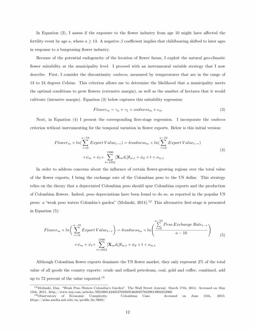
In Equation (2), I assess if the exposure to the flower industry from age 10 might have affected the

fertility event by age a, where a � 13. A negative � coefficient implies that childbearing shifted to later ages

in response to a burgeoning flower industry.

Because of the potential endogeneity of the location of flower farms, I exploit the natural geo-climatic

flower suitability at the municipality level. I proceed with an instrumental variable strategy that I now

describe. First, I consider the discontinuity coolness, measured by temperatures that are in the range of

13 to 24 degrees Celsius. This criterion allows me to determine the likelihood that a municipality meets

the optimal conditions to grow flowers (extensive margin), as well as the number of hectares that it would

cultivate (intensive margin). Equation (3) below captures this suitability regression:

Flower

m

= �

o

+ �1 ⇥ coolness

m

+ ✏

m

(3)

Next, in Equation (4) I present the corresponding first-stage regression. I incorporate the coolness

criterion without instrumenting for the temporal variation in flower exports. Below is this initial version:

Flower

m

⇥ ln(a�10X

⌧=0

Export V alue

t�⌧

) = �coolness

m

⇥ ln(a�10X

⌧=0

Export V alue

t�⌧

)

+ m

+

t

+1990X

t=1952

[Xm

d

t

]✓m,t

+ �

d

⇥ t+ ⌫

m,t

(4)

In order to address concerns about the influence of certain flower-growing regions over the total value

of the flower exports, I bring the exchange rate of the Colombian peso to the US dollar. This strategy

relies on the theory that a depreciated Colombian peso should spur Colombian exports and the production

of Colombian flowers. Indeed, peso depreciations have been found to do so, as reported in the popular US

press: a “weak peso waters Colombia’s garden” (Molinski, 2014).12 This alternative first-stage is presented

in Equation (5):

Flower

m

⇥ ln

✓a�10X

⌧=0

Export V alue

t�⌧

◆= �coolness

m

⇥ ln

a�10P⌧=0

Peso Exchange Rate

t�⌧

a� 10

!

+ m

+

t

+1990X

t=1952

[Xm

d

t

]✓m,t

+ �

d

⇥ t+ ⌫

m,t

(5)

Although Colombian flower exports dominate the US flower market, they only represent 2% of the total

value of all goods the country exports: crude and refined petroleum, coal, gold and coffee, combined, add

up to 72 percent of the value exported.13

12Molinski, Dan. “Weak Peso Waters Colombia’s Garden”. The Wall Street Journal. March 17th, 2014. Accessed on May15th, 2015. http://www.wsj.com/articles/SB10001424052702303546204579439813904252966

13Observatory of Economic Complexity. Colombian Case. Accessed on June 15th, 2015:https://atlas.media.mit.edu/en/profile/hs/0603/

12

4 Data

4.1 Data Sources

For this study, I obtained the data on the female outcomes from the Colombian Demographic Health Surveys

(DHS). The waves that I use belong to the years 1986 (DHS-I), 1990 (DHS-II), 1995 (DHS-III), 2000 (DHS-

IV), 2005 (DHS-V) and 2010 (DHS-VI). The DHS surveyed a subsample of all Colombian municipalities,

covering 446 municipalities out of the existing 1,120. Taking into account that the industry was born in

the year 1965, and that the first fertile age category of interest is age 13, I concentrate on all cohorts born

after 1952 as potentially having seen their sexual initiation, first pregnancy and first marriage affected by

the flower shocks. My sample is thus made of 115,824 females born between 1952 and 1993.14

The DHS surveys are divided into several sections. For this analysis, I extract all the outcomes from

the Individual Recode questionnaire, which covers detailed information about fertility-related events for all

females aged 13 to 50 years old that are residing in the household. Females are asked about the age at which

the first intercourse took place, the age for the first pregnancy and the age for the first union/marriage. I

can then construct their individual histories for being sexually active, pregnant or married from the answers

to those questions.

The questionnaire identifies the municipality of current residence. In addition to that, it also covers

questions for migration spells—years lived in place of residence. This allows me to identify the females that

were already residing in their current location before the age of 10. Migrants are then defined as those

females who moved to their current municipality of residence older than the age of 10. This is important

because I will later conduct a separate analysis contrasting the subsample of residents and migrants.

The data to identify the geographic distribution of flower farms comes from a government registry, publicly

released by the Agriculture and Rural Development Ministry.15 This cross-sectional snapshot is from a year

relatively late in the sample, 2007. As such, the instrumentation for the location of flower farms becomes

crucial. The public registry identifies the geographic location (municipality) of the farms as well as the size

in hectares. The size variable is further broken into hectares cultivated with flowers and foliage. I categorize

a municipality as having the flower status, flower status

m

, if it has, at least, one flower farm cultivating a

positive number of hectares, flower hectares

m

> 0.

To measure the performance of the flower industry, I use three other sources. First, the UN ComTrade

portal has data available for the volume and value of Colombian exports to the world. Second, the US Food

14I restrict the sample to females who are at least 17 years old on the survey year. The last DHS wave is from the surveyyear 2010, hence I can track outcomes for cohorts born up to 1993.

15Flower farms had to be registered for an agricultural program: Incentivo sanitario a las flores y follaje (ISFF), in itsSpanish acronym.

13

and Agricultural Service (FAS)16 has detailed volume and value information for Colombian exports coming

to the US market, expanding a longer period of time than its UN counterpart. Last, there is the work

put together by Marín and Rangel (2000), which combines the yearly bulletins published by the Colombian

Association of Flower Growers (Asocolflores) on several production aggregates. From all sources, I retrieve

the level and value of production whenever available—always measured at the national level. Since I chose

to concentrate on the bilateral trade between Colombia and the US, the analysis will use the data retrieved

from the Food and Agricultural Service (FAS) administration.

I should mention that, in the context of the flower markets, an international price or flower index does not

exist. Given this situation, the own production decisions of Colombian growers directly influence the value

that their flower exports attain in the US market. I will address the concerns about the own determination of

the Colombian export value incorporating the Colombian peso exchange rate (deflated number of Colombian

pesos per US dollar). The exchange rate series comes from the Colombian Central Bank, Banco de la

República.

4.2 Descriptive Statistics

Table 1 presents the summary statistics for the sample of interest. In Panel A, I describe the individual-level

characteristics by flower versus non-flower municipalities. The cohorts I study were born between 1952 and

1993. The average female in my sample is approximately 31 years old, she had her first sexual intercourse

at the age of 18, was married by the age of 20 and had her first baby one year after that, by the age of 21.17

By age 15, approximately one quarter (24.0 percent) of the females had become sexually active; that

fraction increases to 48.1 percent by age 17. This is important because an early sexual initiation might lead

to an early pregnancy: whereas only 7.2 percent of females were pregnant for the first time by age 15, that

figure had increased to 21.5 percent by age 17. That represents a dramatic 200 percent increase. Similarly,

around 9 percent of the females in the sample had entered their first union by age 15, and 21.7 percent of

them had done so by age 17. The sexual debut, first birth and first union probabilities are higher in the

non-flower municipalities as compared to the flower ones.

To help visualize these numbers, in Figure 1a, I look at the evolution of the fraction of females who

have been pregnant by age 15. Here I distinguish two clear periods: (i) spanning the decades 1950s and

1960s, and (ii) from 1970 onwards. As it can be seen, for the cohorts born between 1950 and the end of

the 1960s decade, the fraction of females who had been pregnant by age 15 remained considerably stable at

approximately 6%. Noticeably, starting with the cohorts born in the 1970s, that fraction begins to rise: by16Foreign Agriculture Service, Global Agricultural Trade System (GATS), code 0795AT – fresh cut flowers.17This statistic is computed imposing the restriction that the individual be at least 25 years old on the survey year. This

represents the 90th percentile for the age of first pregnancy.

14

1985, 9.19% of females had been pregnant for the first time by age 15—a 50 percent increase.

Understanding the forces behind the timing of these events, particularly for females going through their

middle adolescence (15-16) and late adolescence years (17-19), is critical to this study. With that aim, I have

plotted the trends by flower suitability in Figure 2. I show the average age for sexual debut, first pregnancy,

and marriage across cohorts and flower-suitable versus unsuitable municipalities from 1940 to 1985.18 No-

ticeably, a strikingly similar pattern is observed across all three events: the series remain remarkably stable

for the cohorts born between 1940 and 1970, and the average ages start declining after that. The early

cohorts in my sample, born in the decade of the 1950s, became sexually active approximately at age 19, and

were pregnant for the first time at age 22. For the later cohorts, born in the 1980s, the average age for sexual

initiation had fallen to 17, and the first pregnancy happened by age 20. This corresponds to a decline of

-10.5% in the sexual initiation age, as well as decline of -9.70% for the age of first pregnancy, over the course

of three decades.

Continuing in Table 1, Panel A, 32.5 percent of the females reside in flower municipalities. Moreover, 47.2

percent migrated to the municipality where they currently reside—migration is defined as having arrived to

the current municipality after the age of 10.

In the second panel of Table 1, Panel B, I present the municipality-level characteristics. The DHS waves

covered a total of 446 municipalities. The average flower municipality in the sample cultivates approximately

74 hectares and has 17.3 flower firms operating. The geographic distribution of these municipalities can be

seen in Figure 3. Two administrative departments19 concentrate 84 percent of flower hectares: Cundinamarca

and Antioquia. For a later robustness analysis it will be useful to keep in mind this geographic subsample,

which is also home to 11 percent of the females interviewed. Appendix Figure A.1 shows the subsample of

DHS municipalities that lie within Cundinamarca and Antioquia, displaying their flower status.

Flower municipalities are closer to the capital of the administrative department, the main market centre

of the region, as well as Bogotá. These metrics are aligned with the logistics of the flower industry but

they also speak about the degree of economic development of flower and non-flower nuclei. In terms of

other agricultural commodities, both flower and non-flower municipalities cultivate coffee, with the former

doing so more intensively. The presence of coal and gold mines is very similar across them, and non-flower

municipalities have a greater presence of petrol reserves. I will interact these municipality covariates with

year dummies and incorporate them to my regressions, as an attempt to capture differential trends by these

characteristics. I will also add linear time trends defined at the department level.

18Again, in order to avoid censoring issues when computing the average age for sexual initiation and average age for firstpregnancy, I condition on females being at least 25 years old in the survey year. Thus, the last birth cohort that I can measureat age 25 was born in 1985.

19An autonomous subdivision of the Colombian territory, higher than the municipality level

15

Last, Panel C of Table 1 presents the annual-level performance of the flower industry. I track the

evolution of flower exports in terms of the level of production (stems) and the export value (millions of

US dollars, deflated by an export price index) from the year 1965 to 2010. On average, the industry grew

annually at a rate of 28.9 percent in value and 25.7 percent in volume. The evolution over time for the

value and volume series is shown in Figure 4a. The volume and value series track each other strongly. In

Figure 4b, I overlap the Colombian peso exchange rate, since the later series will constitute the basis of the

instrumentation strategy. The exchange rate series closely traces the evolution of the value of exports up

to the second half of the 1990s decade. As a reminder, the year 1995 marked the beginning of a somber

period for the flower industry, when the US Commerce Department imposed punitive anti-dumping levies on

Colombian flower producers. Since the beginning of the 2000s decade, the export value and exchange rate

series became mirror images of each other.

Last, Table 2 provides summary statistics of some key differences between flower and non-flower mu-

nicipalities before the takeoff of the flower industry (1965). I show the fertility outcomes for cohorts born

between 1940 and 1950. Although the sample is very reduced, females in the flower industries show evidence

of delayed fertility-related choices: they are slightly older at the age of sexual debut, first union and first

birth; they also have a smaller number of total children. The sexual initiation, first birth and first marriage

probabilities, as of age 15 and age 17, are also lower for the flower cohorts.

5 Results

I begin with the suitability assessment in Table 3, following the regression specified in Equation (3). This

regression was meant to evaluate the geo-climatic suitability of a municipality to become a flower-producing

center. The main regressor of interest is the coolness requirement. Broadly speaking, coolness refers to

whether a municipality has a temperate climate. This is represented by an average annual temperature that

lies in the range of 13 to 24 Celsius. In Columns (1) and (3), I show that coolness significantly affects the

likelihood that the industry will take off in the municipality, as well as the number of hectares.

I consider alternative temperature requirements in Columns (2) and (4). These include: the regressor

hot, which captures average annual temperatures above 24 Celsius, and the regressor cold, for average

annual temperatures below 13 Celsius. Both hot and cold negatively affect the flower suitability, suggesting

that more extreme climates are not flower suitable. In the companion Appendix Table A.1, the suitability

regression is ran on the entire universe of Colombian municipalities, showing that the significance of the

coolness requirement remains robust. For the remaining of the analysis, I will focus on the extensive margin

of cultivation, using the flower status of a municipality.

16

5.1 Reduced Form Evidence

Next, I show the reduced-form relationship between the flower shocks and the timing of the different fertility-

related outcomes. For that, I interact the flower suitability, coolness, of a municipality with a full set of

year-of-birth dummies, and I proceed to regress the probability of the fertility-related event happening by

age a on these interaction terms, always controlling for year-of-birth and municipality fixed effects. In other

words, I run the following regression, Equation (6):

Pregnant by Age ai,m,c,t

= ↵+ Coolnessm

⇥1993X

c=1952

�

c

d

c

+ �

m

+ �

c

+ ✏

i,m,c,t

(6)

The coefficients �c

from these interactions are graphed in Figure 5. I have chosen to display the flower-

year coefficient interactions for the dependent variable “being pregnant”. The pregnancy event is evaluated

at the ages of 15 (top figure) and 17 (bottom figure). To aide the interpretation of the results, I overlay the

value of Colombian flower exports on the year in which each birth cohort turns age a (where age a is either

15 or 17).

These two figures present the first suggestive evidence of the reduced form relationship between the

flower shocks and the timing of the fertility-related events. In Figure 5a, the reduced-form interactions on

pregnancy by age 15 remain considerably stable and oscillate around zero for cohorts born between 1950

to 1970; thereafter, they show a positive tendency. In Figure 5b, I evaluate the pregnancy event by age

17. Noticeably, the relationship between the flower shocks and the likelihood of first pregnancy remains

considerably stable for the birth cohorts spanning the 1950s-1970s, and show a positive, if timid, trend after

that.20

5.2 Sexual Initiation, Pregnancy and Marriage

Now I present the 2SLS regressions. First, Table 4 shows the first-stage coefficients as specified in Equation

(5). The dependent variable for the first-stage is made of the interaction between the flower status of a

municipality and the national performance of the flower industry. As discussed earlier, I have chosen two

measures of performance: (i) the export value of flowers on the year in which the relevant cohort turns age

a; (ii) the cumulative export value from the year in which a cohort turns age 10 to the age of interest a. The

later cumulative value is meant to capture the total exposure from the potential onset of menarche.

To generate shocks to the value of Colombian exports, I use two instruments, each of them specific to

the shock being analyzed. First, to instrument the (log) value of exports on a particular year, I use the

(log) exchange rate of Colombian pesos to the US dollar on that same year. Alternatively, to instrument

20Both graphs in Figures 5a and 5b have the same scale to ease the visualization of the RF flower-year interactions.

17

the cumulative value, I compute the (log) average exchange rate prevailing during the relevant years that

are being added. As explained, the flower status of a municipality will be instrumented via the coolness

non-linear criterion.

In Table 4, Columns (1) and (2) show the first-stage for the year shocks on age 15 and age 17, respectively.

In Columns (3) and (4) I present the cumulative measure of performance by age 15 and age 17. As it can

be seen across all four results, the interaction of the coolness criterion and the exchange rate significantly

affects the growth in the value of flower exports. The first-stage result reported in Column (1) suggests

that a 10 percent increase in the Colombian peso exchange rate (which results in a depreciation of the peso)

significantly increases the value of Colombian flower exports on that particular year by 1.09 percent (log on

log) on flower suitable municipalities. The positive coefficients are aligned with the standard international

trade theory, whereby a depreciated peso should encourage US consumers to purchase Colombian flowers.

The coefficients remain statistically significant and positive across both age categories and the two measures

of performance. Despite the instrument being highly significant, the associated F-statistic is only above

the threshold of 10, as discussed by Staiger and Stock (1997), when using the aggregate measure of flower

performance, in Column (2).

Having established the basis for the first-stage, I continue to present the main set of 2SLS results on Table

5 and 6, following the regressions in Equations (1) and (2), respectively. I analyze the differential impact

of shocks to the flower industry on three outcomes of interest: (i) sexual initiation, (ii) being pregnant, and

(ii) being married for the first time by a particular age a, where a 2 [13, 25]. I have chosen to restrict the

analysis to the age range 13 to 25 with the aim to cover both the age when females begin menstruating and

the age when adolescence can be considered finished. For the sake of clarity, I reports the impact of the

flower shocks at two ages: age 15 (Panel A) and age 17 (Panel B).

Table 5 shows the year-shocks, whereas Table 6 presents the cumulative measure of performance. I have

already explained that the later is an alternative measure aiming to capture the total exposure to the flower

industry, aggregated from age 10 to age 15, or to age 17, respectively. I first report the OLS estimates on

sexual initiation, pregnancy and marriage in Columns (1), (4) and (7), respectively. The OLS coefficients

show that an increase in the value of Colombian flower exports is positively associated with the likelihood

that a female is sexually active, pregnant or married by ages 15 and 17.

Going back to Table 5, note that for each of the two age categories (15 and 17) and each outcome, I

present the base 2SLS coefficients for the (log) year shock in Columns (2), (5), and (8). The base specification

always incorporates municipality and cohort fixed effects. I then build on the base specification, incorporating

differential trends by municipality characteristics in Columns (3), (6) and (9). I begin the IV analysis with the

sexual initiation event. In Columns (2) and (3), it can be seen that the flower shocks significantly increased

18

the probability that a cohort would have had sexual intercourse by age 15, and also by age 17, differentially

in flower suitable municipalities. The 2SLS are all positive, statistically significant and of a higher order

of magnitude than the corresponding OLS counterparts. The coefficient of 0.0682 in Panel A-Column (3)

suggests that a 10 percent increase in the value of Colombian exports on the year in which a female turns age

15 leads to an approximate differential increase of 0.6820 percentage points (pp) in the probability of being

sexually active. This translates to an increase of 2.81 % more above the mean probability over the sample

period, which stands at 0.24 (24.0 percent of females in the sample have had sexual intercourse by age 15).

If I assess the impact on the probability of being sexually active by age 17, a 10 percent increase in the

cumulative export value from age 10 to age 17 leads to an increase of 1.037 percentage points. The results

remain robust to controlling for differential trends by municipality characteristics (including the distance to

the closest international airport, and an index of rural versus urban development), as well as the inclusion of

regional linear time trends. Later on, I will also show that the results remain robust to two other additional

checks: (i) comparing the sample of females for whom I know their migration history, and (ii) restricting my

analysis to the two departments that concentrate flower production.

First intercourse initiates the exposure to pregnancy period, which I analyze next. Columns (4), (5) and

(6) of Table 5 report the flower impact on the probability of being pregnant for the first time, again evaluated

at age 15 (Panel A) and at age 17 (Panel B). I find results that are very much aligned with those reported

for the initiation to sexual activity: positive shocks to the flower industry increase the probability that a girl

is pregnant for the first time in flower suitable municipalities significantly by age 15 and 17.

The 0.0598 coefficient on Panel B -Column (6) implies that a 10 percent increase in the value of Colombian

flower exports will result in an increase of 0.598 percentage points (pp) in the probability that a girl in late-

puberty (age 17) is pregnant. This corresponds to a 2.78% increase above the mean probability over the

sample period (21.5 percent of females had been pregnant for the first time by age 17). The impact evaluated

by age 15 is also positive, albeit it becomes insignificant once I control for the differential trends: a 10 percent

increase in the value of exports results in a 4.85% increase in the probability that a female would be pregnant

by age 15. It should be noted that the magnitude of the coefficients for the age 17 category is higher than

those by age 15 in absolute terms. Nonetheless, the impact in percentage terms (relative to the sample

mean of the event taking place by age a) is attenuated by the fact that the fraction of females who meet the

pregnancy condition is increasing with age. In fact, sexual initiation, pregnancy and marriage are very close

to being universal events in the lives of Colombian women.

To aide the interpretation of the pregnancy outcomes I have put this figure into context: the value of

Colombian exports to the US grew at an average rate of 28 percent per year from 1965 to 2010. As such,

the 2SLS coefficients imply a differential increase of 2.90 percentage points in the probability that a female

19

is sexually active by age 17, and a differential increase of 1.67 percentage points (pp) in the probability she

is pregnant by age 17 in flower suitable municipalities. These results are worth discussing. Previous studies

conducted in the maquila context, the Bangladeshi ready-made garments, or the BPO centers in India, had

suggested that these modern-factory type of jobs were emblematic of a changing fertility pattern for females,

one that allowed them to delay childbirth. In the Colombian rose industry, I find quite the opposite results:

positive flower shocks hastened the entry to motherhood. The childbearing shift to earlier ages suggest a

dominance of the positive income effect, over an opposing substitution effect, in the Colombian case.

Last, Columns (7), (8) and (9) of Table 5 assess the likelihood that a female will be married by ages 15

and 17, respectively. The probability of marriage is positive but not statistically significant when evaluated

at age 15. The impact turns to significant at age 17, and it shares a similar magnitude with the pregnancy

coefficients. This is not surprising since the average age of inception lags the union decision very closely.

In Table 6, I repeat the same exercise, but instead of using the year-level shocks, I use the cumulative

flower shocks, which are aggregated from age 10 to age 15, or to age 17, respectively. The results remain

robust to using this alternative measure of performance. Age of sexual debut, childbearing and union all

shifted to earlier ages in response to the burgeoning flower industry.

5.3 Resident and Migrant Subsamples

Next, I begin a series of robustness exercises. First, I conduct a separate analysis for the sample of residents

and the sample of migrants. Residents are females who were already present in their current municipality

before the age of 10. This threshold was established because the outcomes analyzed comprise the puberty

and early adolescence years, and being able to map the municipality where the females were residing during

this period is crucial to assess if they were indeed affected by the flower industry shocks or not. From the

data, approximately 47.2 percent of the females moved to their current municipality at some point after

they were already 10 years old—unfortunately, I cannot track where the migrants were before they arrived

to their current municipality.

In Table 7, I report the 2SLS for the sexual initiation, pregnancy and marriage outcomes across residents

and migrants. Again I evaluate the likelihood of these three events happening by ages 15 and 17 in Panel

A and Panel B, respectively. Remarkably, the results remain highly significant and of similar magnitudes,

albeit more imprecise, for the sample of residents only. Distinctly, the impact on migrants is statistically

insignificant. This is not surprising, since the municipalities where the migrants spent their adolescence is

unknown, and thus, I should not expect any impact of the flower industry on them.

20

5.4 Geographical Restrictions: Cundinamarca and Antioquia

As discussed earlier, the flower industry penetrated two administrative departments, Cundinamarca and

Antioquia. These two departments concentrate up to 84 percent of flower production, measured in terms of

hectares cultivated. Appendix Figure A.1 shows the subsample of DHS municipalities that lie within Cund-

inamarca and Antioquia, displaying their flower status. Appendix Table A.2 shows the descriptive statistics

for the sample of females in Cundinamarca and Antioquia, as well as the comparison of the municipality-level

characteristics within these two departments.

In Table 8, I present the 2SLS results using this geographic subsample. The relevant comparison is

now across flower and non-flower municipalities that lie within Cundinamarca or Antioquia. The number

of municipalities is reduced to 101, but the results remain consistent: the flower shocks accelerated the

initiation to sexual activity, path to pregnancy and marriage.

5.5 Further Robustness Checks

Last, in Appendix Table A.3, I show that the results remain robust to computing the cumulative exposure

to the flower industry across different age ranges: from age 6, from age 10, or from age 13.

6 Conclusions

This paper has studied the impact of expanding semi-skilled agro-industrial employment opportunities on

outcomes that significantly affect the lives and economic role of young females in Colombia. Using the fresh-

cut flower industry, I present evidence of how economic development, in the form of export-oriented jobs,

affected their fertility timing decisions.

I offer new insights into how the transition from childhood to puberty, and early adulthood, can be shaped

by international trade forces. The results that I find indicate that the increasingly available employment

opportunities precipitated the entrance into early motherhood. These modern factory-type jobs, the epitome

of globalization, accelerated the timing of early sexual and reproductive decisions for very young women.

These results might help explain the so-called “paradox” that is observed in the case of Colombia. Despite

the fact that total fertility (births per woman) has been declining over the entire period of analysis, from

6.56 births per woman observed in 1965 to 2.29 by 2013 (United Nations Population Division, 2014), this

hasn’t been accompanied by a parallel delay in the age for childbearing.

21

In the literature, increasing job opportunities for females has been shown to improve their bargaining

power and their exercise of agency. In contrast to previous studies, which had found evidence of delayed

responses in fertility timing and union formation, the rose industry in Colombia accelerated sexual initi-

ation, union and motherhood. The flower exports brought along secure and permanent income earning

opportunities, particularly for women. As mentioned, if children are normal goods, in principle, this should

lead to increases in the demand for children, via income effects. This could also happen if females have an

intrinsic desire (shaped by social and religious norms) to be early mothers, but were lacking the financial

security and stability to do so. In addition to that, the increased economic and financial stability may

have also contributed to erode any stigma associated with early pregnancies. Further, booming periods may

have indirectly affected the perception of both present and future economic stability, thereby accelerating

motherhood. Despite the fact that the new employment opportunities translate into a higher cost of female

time, the opposing substitution effect was not strong enough to delay the childbearing timing. As such, my

estimates imply a dominance of an income effect over a substitution effect.

Taken together, the results suggest that fertility and nuptiality timing are closely interwoven to the trade

dictums, and that the direction of this relationship might be context specific. Understanding how to affect

adolescent fertility patterns remains an open question that calls for further research.

22

References

[1] Amador, Diego, Raquel Bernal, and Ximena Peña. 2012. “The Rise in Female Participation in Colombia:

Children, Education or Marital Status”. Background Paper. The World Development Report 2012. World

Bank.

[2] Ambrus, Steven. 1994. “International Business : U.S. Ruling a Thorn in Colombian Rose Growers’

Side : Trade: Commerce Department decision imposes punitive anti-dumping levies”. Los Angeles

Times, October 20, 1994. Accessed June 17, 2015. http://articles.latimes.com/1994-10-20/business/fi-

52664_1_colombian-rose

[3] Amin, Sajeda, Ian Diamond, Ruchira T. Naved and Margaret Newby. 1998. “Transition to Adulthood

of Female Garment-Factory Workers in Bangladesh”. Studies in Family Planning. 29:2, pp 185-200.

[4] Antman, Francisca. 2014. “Spousal Employment and Intra-Household Bargaining Power”. Working Pa-

per.

[5] Atkin, David. 2009. “Working for the Future: Female Factory Work and Child Health in Mexico”.

Working Paper.

[6] Atkin, David. 2012. “Endogenous Skill Acquisition and Export Manufacturing in Mexico”. Working

Paper.

[7] Bozon, Michel, Cecilia Gayet and Jaime Barrientos. 2009. “A Life Course Approach to Patterns and

Trends in Modern Latin American Sexual Behaviour”. Journal of Acquired Immune Deficiency Syn-

dromes. 51(1).

[8] Bureau of International Labor Affairs. 2002. “Colombia: Laws Governing Exploitative Child Labor.

Report”. U.S. Department of Labor.

[9] Dolan, Catherine. 2007. “Assembling Flowers and Cultivating Homes: Labor and Gender in Colombia.

Book Review”. Feminist Economics. 13:2, 210-215.

[10] Duflo, Esther. 2012. “Women Empowerment and Economic Development”. Journal of Economic Liter-

ature. 50(4), pp. 1051–1079.

[11] Elson, D. and Pearson, R. 1981. “Nimble fingers make cheap workers: An analysis of women’s employ-

ment in third world export manufacturing”. Feminist Review. 7, Spring: 87-107.

23

[12] Encyclopedia Britannica Online. Colombia. Retrieved 25 November, 2013,

http://www.britannica.com/EBchecked/topic/126016/Colombia

[13] Figueroa, Alicia, Adriana Lima and Elizabeth McCraken. 2012. “Are Colombian Flowers Experiencing

a US drought?”. Knowledge@Wharton article series. Wharton School of the University of Pennsylvania.

[14] Friedemann-Sánchez, Greta. 2006. Assembling Flowers and Cultivating Homes: Labor and Gender in

Colombia. Lanham: Lexington Books, 2006.

[15] Heath, Rachel, and A. Mushfiq Mobarak. 2015. “Manufacturing Growth and the Lives of Bangladeshi

Women”. Journal of Development Economics, 115, 1-15.

[16] Hotz, V. Joseph, Jacob Alex Klerman and Robert J. Willis. 1997. “The Economics of Fertility in Devel-

oped Countries”. Handbook of Population and Family Economics. Edited by M.R. Rosenzweig and O.

Stark.

[17] International Bureau of Education (IBE). United Nations Educational, Scientific and Cul-

tural Organization (UNESCO). 2010. World Data on Education - Colombian Case. Document:

IBE/2010/CP/WDE/ck

[18] International Labor Office (ILO). 2006. “Colombia: Child Labor Data Country Brief”. International

Program on the Elimination of Child Labor (IPEC).

[19] Jayachandran, Seema. 2015. “The Roots of Gender Inequality in Developing Countries”. Annual Review

of Economics, Volume 7: Submitted. DOI: 10.1146/annurev-economics-080614-115404.

[20] Jensen, Robert. 2012. "Do Labor Market Opportunities Affect Young Women’s Work and Family De-

cisions? Experimental Evidence from India," Quarterly Journal of Economics, 127(2), p. 753-792.

[21] Jensen, Robert. 2010. “The (Perceived) Returns to Education and the Demand for Schooling". Quarterly

Journal of Economics, 125(2), p. 515-548.

[22] Korovkin, Tanya. 2003. “Cut Flower Exports, Female Labor, and Community Participation in Highland

Ecuador”. Latin American Perspectives, Vol. 30, No. 4, pp 18-42.

[23] Majlesi, Kaveh. 2015. “Labor Market Opportunities and Sex-Specific Investment in Children’s Human

Capital: Evidence from Mexico”. Working Paper.

[24] Mammen, Kristin, and Christina Paxon. 2000. “Women’s Work and Economic Development”. The Jour-

nal of Economic Perspectives, 14:4, 141-164.

24

[25] Marín Ángel, M.J. , and J.E. Rangel Aceros. 2000. “Comercialización Internacional de Flores: An-

tecedentes y Evolución 1990-1999”. Dissertation, Universidad Nacional de Colombia.

[26] Meier, V. 1999. “Cut-Flower production in Colombia—a major development success story for women?”.

Environment and Planning. Vol. 31, pp 273-289.

[27] Méndez, José. 1991. “The Development of the Colombian Cut Flower Industry”. Working Papers on

Trade Policy, WPS 660. The World Bank.

[28] Miller, Grant. 2005. “Contraception as Development? New Evidence from Family Planning in Colombia”.

NBER Working Paper 11704.

[29] Miller, Grant, and B. Piedad Urdinola. 2010. “Cyclicality, Mortality and the Value of Time: The Case

of Coffee Price Fluctuations and Child Survival in Colombia”. Journal of Political Economy. 118: 1,

113-155.

[30] Ministry of Agriculture and Rural Development and Asocolflores. 2008. Colombian Grown: The Finest

Quality Cut Flowers in the World. Diseño Editorial.

[31] Molinski, Dan. “Weak Peso Waters Colombia’s Garden”. The Wall

Street Journal. March 17th, 2014. Accessed on May 15th, 2015.

http://www.wsj.com/articles/SB10001424052702303546204579439813904252966

[32] Oster, Emily, and Bryce Millett Steinberg. 2013. “Do IT Service Centers Promote School Enrollment?

Evidence from India”. Journal of Development Economics. 104, 123-135.

[33] Pun, Ngai. Made in China: Women Factory Workers in a Global Workplace. Duke University Press,

2005. Durham, NC.

[34] Qian, Nancy. 2008. “Missing Women and The Price of Tea in China: The Effect of Sex-Specific Earnings

on Sex Imbalance”. The Quarterly Journal of Economics. 123:3, 1251-1285.

[35] Rosero-Bixby, Luis, Teresa Castro-Martín and Teresa Martín-García. 2009. “Is Latin America Starting

to Retreat from Early and Universal Childbearing?”. Demographic Research. 20:9, 169-194.

[36] Schultz, T. Paul. 1985. “Changing World Prices, Women’s Wages, and the Fertility Transition: Sweden,

1860-1910”. Journal of Political Economy. 93:6, pp 1126-1154.

[37] Sivasankaran, Anitha. 2014. “Work and Women’s Marriage, Fertility and Empowerment: Evidence from

Textile Mill Employment in India”. Job Market Paper.

25

[38] Spano, Sedra. 2004. “Stages of Adolescent Development”. ACT for Youth Upstate Center of Excellence.

Cornell University.

[39] Talcott, Molly. 2004. “Gendered Webs of Development and Resistance: Women, Children, and Flowers

in Bogotá”. Signs. 29:2, 465-489.

[40] United Nations Population Fund (UNFPA). “State of the World Population, 2014”. Accessed online

on June 15th, 2015. http://www.unfpa.org/sites/default/files/pub-pdf/EN-SWOP14-Report_FINAL-

web.pdf

[41] United Nations Population Fund (UNFPA). 2013. “Adolescence Pregnancy: A Review of the Evidence”.

Prepared by Edilberto Loaiza and Mengjia Lang.

[42] Urrutia, Miguel. 1985. Winners and Losers in Colombia’s Economic Growth of the 1970s. New York:

Oxford University.

[43] World Health Organization (WHO). 2014. “Adolescent Pregnancy”. Fact Sheet N 364. Web Resource.

Accessed on June 2014. http://www.who.int/mediacentre/factsheets/fs364/en/

26

Figure 1: Trends in Fertility-Related Outcomes in Colombia

Flower Cohorts: they turn age 13 in 1965 and thereafter

.05

.06

.07

.08

.09

.1F

ract

ion P

regnant by

Age 1

5

.15

.2.2

5.3

.35

Fra

ctio

n S

exu

ally

Act

ive b

y A

ge 1

5

1950 1960 1970 1980Birth Cohort

Fraction Sexually Active by Age 15

Fraction Pregnant by Age 15

Figure 1a: Sexually Active and Pregnant by age 15

16

17

18

19

20

Ave

rage A

ge

12

34

56

Ave

rage N

um

ber

of C

hild

ren

1940 1945 1950 1955 1960 1965 1970 1975 1980 1985Year of Birth

Average Number of Children

Average Age for Sexual Initiation

Figure 1b: Fertility and Sexual Initiation

Top Figure shows two time series: (i) the fraction of females who initiatied sexual activity (left-axis), and (ii) females whohad been pregnant for the first time (right-axis), by birth cohort. These two events are evaluated by age 15. I identify with avertical line the birth cohort born in 1952. This cohort turned age 13 (puberty period) in the year 1965, which marks the firstshipment of fresh-cut Colombian flowers to the US. Thus, cohorts born after 1952 reached their age of menarche in a worldwhere the flower industry was already operating.The bottom figure shows the evolution for the average age at sexual debut andthe average number of children. The average age is computed using the sample of females who are at least 25 years old on thesurvey year. Bottom Figure Source: Colombia DHS surveys 1986, 1990, 1995, 2000, 2005 and 2010.

27

Figure 2: Trends by Flower Suitability

Flower Cohorts: they turn age 13 in 1965 and thereafter

16

17

18

19

20

21

Ave

rage A

ge for

First

Inte

rcours

e

1940 1950 1960 1970 1980Year of Birth

Non!Suitable for Flowers

Flower Suitable

Flower Cohorts: they turn age 13 in 1965 and thereafter

17

18

19

20

21

22

23

Ave

rage A

ge for

First

Pre

gnancy

1940 1950 1960 1970 1980Year of Birth

Non!Suitable for Flowers

Flower Suitable

Flower Cohorts: they turn age 13 in 1965 and thereafter

17

18

19

20

21

22

23

Ave

rage A

ge for

First

Unio

n

1940 1950 1960 1970 1980Year of Birth

Non!Suitable for Flowers

Flower Suitable

Figures separately track the average age for sexual initiation, first pregnancy, and union by birth cohort and acrossflower suitable municipalities. I identify with a vertical line the birth cohort born in 1952. This cohort turned age 13(puberty period) in the year 1965, which marks the first shipment of fresh-cut Colombian flowers to the US. Thus,cohorts born after 1952 reached their age of menarche in a world where the flower industry was already operating.Source: Colombia DHS surveys 1986, 1990, 1995, 2000, 2005 and 2010.

28

Figure 3: Distribution of Flower Municipalities

LegendFlower

Non-Flower

Not on DHS surveys

This figure shows the municipalities that were surveyed in any of the Colombian DHS waves (survey years: 1986,1990, 1995, 2000, 2005 or 2010). In red, I identify the municipalities cultivating flowers as of 2007. The flowermunicipalities are those municipalities that have at least one flower farm, cultivating a positive number of flowerhectares, hectares > 0. Sources: Shape-file from DANE; flower hectare distribution from the Ministry of Agricultureand Rural Development. Demographic and Health Surveys (DHS).

29

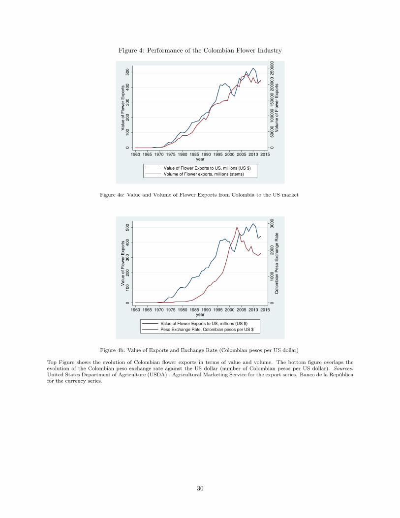
Figure 4: Performance of the Colombian Flower Industry

050000

100000

150000

200000

250000

Volu

me o

f F

low

er

Exp

ort

s

0100

200

300

400

500

Valu

e o

f F

low

er

Exp

ort

s

1960 1965 1970 1975 1980 1985 1990 1995 2000 2005 2010 2015year

Value of Flower Exports to US, millions (US $)

Volume of Flower exports, millions (stems)

Figure 4a: Value and Volume of Flower Exports from Colombia to the US market

01000

2000

3000

Colo

mbia

n P

eso

Exc

hange R

ate

0100

200

300

400

500

Valu

e o

f F

low

er

Exp

ort

s

1960 1965 1970 1975 1980 1985 1990 1995 2000 2005 2010 2015year

Value of Flower Exports to US, millions (US $)

Peso Exchange Rate, Colombian pesos per US $

Figure 4b: Value of Exports and Exchange Rate (Colombian pesos per US dollar)

Top Figure shows the evolution of Colombian flower exports in terms of value and volume. The bottom figure overlaps theevolution of the Colombian peso exchange rate against the US dollar (number of Colombian pesos per US dollar). Sources:United States Department of Agriculture (USDA) - Agricultural Marketing Service for the export series. Banco de la Repúblicafor the currency series.

30

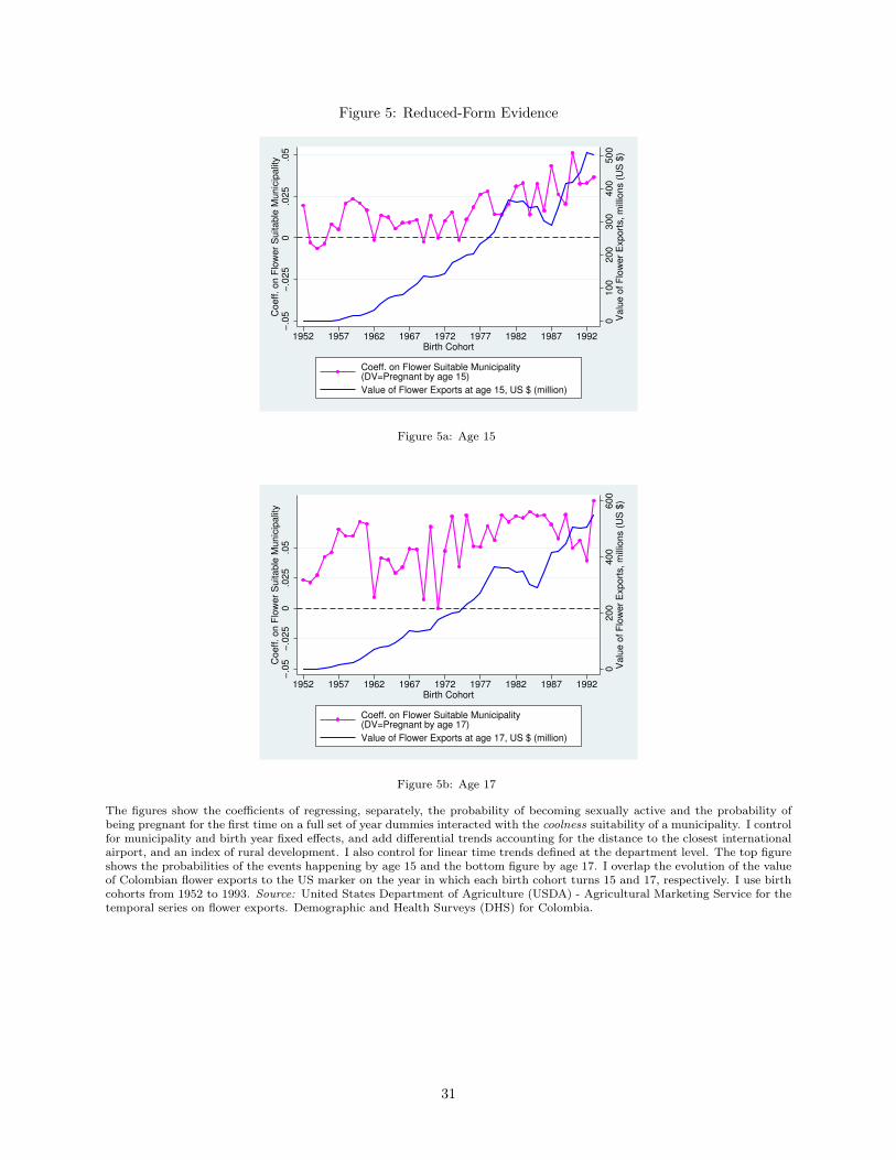
Figure 5: Reduced-Form Evidence

0100

200

300

400

500

Valu

e o

f F

low

er

Exp

ort

s, m

illio

ns

(US

$)

!.0

5!

.025

0.0

25

.05

Coeff. on F

low

er

Suita

ble

Munic

ipalit

y

1952 1957 1962 1967 1972 1977 1982 1987 1992Birth Cohort

Coeff. on Flower Suitable Municipality(DV=Pregnant by age 15)

Value of Flower Exports at age 15, US $ (million)

Figure 5a: Age 15

0200

400

600

Valu

e o

f F

low

er

Exp

ort

s, m

illio

ns

(US

$)

!.0

5!

.025

0.0

25

.05

Coeff. on F

low

er

Suita

ble

Munic

ipalit

y

1952 1957 1962 1967 1972 1977 1982 1987 1992Birth Cohort

Coeff. on Flower Suitable Municipality(DV=Pregnant by age 17)

Value of Flower Exports at age 17, US $ (million)

Figure 5b: Age 17

The figures show the coefficients of regressing, separately, the probability of becoming sexually active and the probability ofbeing pregnant for the first time on a full set of year dummies interacted with the coolness suitability of a municipality. I controlfor municipality and birth year fixed effects, and add differential trends accounting for the distance to the closest internationalairport, and an index of rural development. I also control for linear time trends defined at the department level. The top figureshows the probabilities of the events happening by age 15 and the bottom figure by age 17. I overlap the evolution of the valueof Colombian flower exports to the US marker on the year in which each birth cohort turns 15 and 17, respectively. I use birthcohorts from 1952 to 1993. Source: United States Department of Agriculture (USDA) - Agricultural Marketing Service for thetemporal series on flower exports. Demographic and Health Surveys (DHS) for Colombia.

31

Table 1: Descriptive Statistics across Flower vs Non-Flower

Non-Flower Flower

Panel A: Individual-Level Characteristics Mean SD Mean SDAge 30.834 9.396 30.690 9.312Birth Year 1973.582 10.463 1971.799 10.602Age became sexually active 18.056 3.754 18.455 3.725Age at first marriage 20.190 4.897 21.105 4.945Age at first birth 21.244 4.441 21.990 4.565Sexually active by age 15 0.253 0.435 0.212 0.409Sexually active by age 17 0.495 0.500 0.452 0.498Pregnant by age 15 0.081 0.272 0.053 0.223Pregnant by age 17 0.234 0.423 0.175 0.380Married by age 15 0.100 0.300 0.059 0.236Married by age 17 0.241 0.428 0.165 0.371Resides in Cundinamarca or Antioquia 0.070 0.255 0.197 0.398Migrated after age 10 0.486 0.500 0.443 0.497Females 78135 37679

Non-Flower Flower

Panel B: Municipality-Level Characteristics Mean SD Mean SDMunicipalities 369 77Flower Hectares 0 0 74.408 163.029Coffee hectares 766.686 1608.147 1758.687 2380.470Gold (Dummy) 0.176 0.381 0.208 0.408Coal (Dummy) 0.103 0.304 0.104 0.307Distance to capital of department (km) 80.427 62.126 54.464 44.948Distance to Bogotá (km) 374.224 209.132 172.330 102.925Distance to main market center (km) 145.067 125.026 51.017 43.631Rurality Index 0.534 0.251 0.385 0.254

Panel C: Annual-Level Flower Variables Mean SDValue of Flower Exports (US$ millions) 230.853 173.984Growth in Value of Flower Exports 0.289 0.605Volume of Flower Exports (stems, 1000s) 97041.833 78795.090Growth in Volume of Flower Exports 0.257 0.432Exchange Rate (Colombian Peso per US $ ) 837.036 950.075Growth in the Exchange Rate 0.125 0.120Note: All DHS waves. The variables for the average age for sexual initiation, first birth and marriage are definedfor the sample of females who were older than 25 years old in the survey year. This represents the 90th percentilefor age of first pregnancy (birth delivery).

32

Table 2: Individual Characteristics for Pre-Flower Cohorts 1940 - 1950

Non-Flower Flower

Pre-Flower Arrival Individual Characteristics Mean SD Count Mean SD CountBirth Year 1945.729 3.101 2028 1945.634 3.055 1768Age 44.947 3.013 2028 44.821 3.084 1768Age became sexually active 18.733 4.668 1412 19.879 5.176 1114Age at first marriage 20.116 5.276 1891 21.077 5.477 1618Age at first birth 21.585 4.965 1891 22.493 5.140 1636Total children ever born 5.102 3.196 2028 3.753 2.543 1768Sexually active by age 15 0.243 0.429 1476 0.164 0.371 1188Sexually active by age 17 0.437 0.496 1476 0.324 0.468 1188Pregnant by age 15 0.093 0.290 2028 0.057 0.232 1768Pregnant by age 17 0.238 0.426 2028 0.185 0.388 1768Married by age 15 0.127 0.333 2028 0.085 0.280 1768Married by age 17 0.277 0.448 2028 0.210 0.408 1768

Note: Individual-level characteristics for the sample of females who were born between 1940 and 1950, prior to the adventof the flower industry (1965).

33

Table 3: Flower Suitability

Flower Status Flower Hectares

(1) (2) (3) (4)

Coolness 0.302⇤⇤⇤ 24.423⇤⇤⇤(0.034) (7.195)

Hot -0.308⇤⇤⇤ -24.920⇤⇤⇤(0.033) (6.932)

Cold -0.232⇤⇤⇤ -12.651(0.072) (13.562)

Constant 0.030⇤⇤⇤ 0.327⇤⇤⇤ 1.292 25.064⇤⇤⇤(0.011) (0.032) (1.069) (6.931)

Municipalities 446 446 446 446R-Squared 0.159 0.160 0.028 0.028F-Stat 77.344 42.925 11.524 7.016⇤p < 0.10, ⇤⇤

p < 0.05, ⇤⇤⇤p < 0.01

Note: Note: robust standard errors reported in parentheses. I presentthe OLS results to evaluate the suitability of a municipality for flowercultivation. The outcome variables reflect both the extensive margin offlower cultivation, flower status, as well as the intensive margin, flowerhectares. The flower status and flower hectares are measured at the mu-nicipality level. The flower status identifies whether a municipality is aflower-producing center or not. Hectares corresponds to the number ofhectares under flower cultivation. The suitability requirement exploits adiscontinuity in temperature: coolness. It captures whether the averageannual temperature lies between 13-24 Celsius (55-75 F), deemed to beoptimal for flower growth. I add a dummy Hot for temperatures thatexceed 24 Celsius and a dummy Cold for temperatures that are below13 Celsius as alternative suitable requirements. The sample includes allmunicipalities that were surveyed across subsequent DHS waves.

34

Table 4: First-Stage Results for Flower Shocks

Flower Status *(Log) Export Value Flower Status *(Log) Cumulativeon the year you turned Export Value from age 10

age a up to age a

age 15 age 17 age 15 age 17

(1) (2) (3) (4)

Coolness ⇥ (Log) Exchange Rate at age 15 0.1093⇤⇤⇤(0.0421)

Coolness ⇥ (Log) Exchange Rate at age 17 0.1109⇤⇤⇤(0.0343)

Coolness ⇥ (Log) Average Exchange Rate from age 10 to 15 0.1129⇤⇤(0.0543)

Coolness ⇥ (Log) Average Exchange Rate from age 10 to 17 0.1197⇤⇤⇤(0.0451)

Individuals 115814 115814 115814 115814Municipalities 446 446 446 446Years 42 42 42 42R-Squared 0.973 0.986 0.976 0.987F-stat 6.746 10.487 4.326 7.043⇤p < 0.10, ⇤⇤

p < 0.05, ⇤⇤⇤p < 0.01

Note: standard errors clustered at the municipality level are shown in parentheses. The dependent variable for the first-stage consists of the status of a municipalityinteracted with the (log) performance of Colombian flower exports. Measures of performance include the (log) value of exports on a given year or, alternatively,the (log) cumulative value of Colombian flower exports from the year a female turns 10 to the age of interest a. The instrument is made of the interaction of the(log) average Colombian peso exchange rate and the coolness requirement for flower suitability (temperature criterion between 13-24 Celsius). All specificationsinclude municipality, year, and DHS wave fixed effects. I also control for the type of municipality (urban versus rural). I include differential trends based onmunicipality characteristics. For that, I interact year dummies with the closest international airport (Bogotá or Medellín), as well as with a rurality index. I addlinear time trends at the Department level. The birth years span from 1952 to 1993. Source: DHS wave of 1986, 1990, 1995, 2000, 2005 and 2010.

35

Table 5: OLS and 2SLS for the year-shocks on age a: 15 and 17

Panel A: By age 15 Sexually Active Pregnant Married

OLS 2SLS 2SLS OLS 2SLS 2SLS OLS 2SLS 2SLS

(1) (2) (3) (4) (5) (6) (7) (8) (9)Flower ⇥ (Log) Value at age 15 0.0144⇤⇤⇤ 0.0554⇤⇤⇤ 0.0682⇤ 0.0010 0.0133⇤ 0.0349 0.0004 0.0082 0.0345

(0.0020) (0.0190) (0.0386) (0.0011) (0.0080) (0.0219) (0.0013) (0.0070) (0.0230)

Panel B: By age 17 Sexually Active Pregnant Married

OLS 2SLS 2SLS OLS 2SLS 2SLS OLS 2SLS 2SLS

(1) (2) (3) (4) (5) (6) (7) (8) (9)Flower ⇥ (Log) Value at age 17 0.0293⇤⇤⇤ 0.1159⇤⇤⇤ 0.1037⇤⇤ 0.0069⇤⇤ 0.0361⇤ 0.0598⇤ 0.0030 0.0260 0.0599⇤

(0.0047) (0.0421) (0.0481) (0.0027) (0.0186) (0.0349) (0.0026) (0.0169) (0.0323)

Individuals 106966 106966 106966 115814 115814 115814 115814 115814 115814Municipalities 446 446 446 446 446 446 446 446 446Years 42 42 42 42 42 42 42 42 42Differential Trends Yes Yes Yes⇤p < 0.10, ⇤⇤

p < 0.05, ⇤⇤⇤p < 0.01

Note: standard errors clustered at the municipality level are shown in parentheses. The dependent variables include the likelihood that a female is sexuallyactive, pregnant or married by age a, where age here refers to 15 or 17 years old. These outcomes are regressed on the interaction between the flower status ofa municipality and the (log) peformance of the flower industry. Measures of performance include the (log) value of the flower exports on that particular yearor the (log) cumulative value of Colombian flower exports to the US from the year a female turns 10 to the relevant age of interest a. The instrument is madeof the interaction of the (log) average Colombian peso exchange rate and the coolness requirement for flower suitability (temperature criterion between 13-24Celsius). All specifications include municipality, year, DHS-wave, and rurality (urban vs rural dummy) fixed effects. Further, I include differential trendsbased on municipality characteristics. For that, I interact year dummies with the closest international airport (Bogotá or Medellín), as well as with a ruralityindex. I add linear time trends at the Department level. The sample is made of females who are between ages 17 and 50 on the survey year. The birth yearsspan from 1957 to 1993. Source: DHS wave of 1986, 1990, 1995, 2000, 2005 and 2010.

36

Table 6: OLS and 2SLS for the accumulated flower shocks on age a: 15 and 17

Panel A: By age 15 Sexually Active Pregnant Married

OLS 2SLS 2SLS OLS 2SLS 2SLS OLS 2SLS 2SLS

(1) (2) (3) (4) (5) (6) (7) (8) (9)Flower ⇥ (Log) Accumulated Value 0.0118⇤⇤⇤ 0.0467⇤⇤⇤ 0.0820⇤ 0.0008 0.0115⇤ 0.0425 0.0004 0.0069 0.0379from age 10 to 15 (0.0017) (0.0158) (0.0467) (0.0009) (0.0066) (0.0270) (0.0011) (0.0057) (0.0261)

Panel B: By age 17 Sexually Active Pregnant Married

OLS 2SLS 2SLS OLS 2SLS 2SLS OLS 2SLS 2SLS

(1) (2) (3) (4) (5) (6) (7) (8) (9)Flower ⇥ (Log) Accumulated Value 0.0227⇤⇤⇤ 0.0901⇤⇤⇤ 0.1083⇤⇤ 0.0053⇤⇤ 0.0279⇤⇤ 0.0633⇤ 0.0021 0.0199 0.0615⇤from age 10 to 17 (0.0038) (0.0317) (0.0536) (0.0022) (0.0139) (0.0380) (0.0021) (0.0127) (0.0344)

Individuals 106966 106966 106966 115814 115814 115814 115814 115814 115814Municipalities 446 446 446 446 446 446 446 446 446Years 42 42 42 42 42 42 42 42 42Differential Trends Yes Yes Yes⇤p < 0.10, ⇤⇤

p < 0.05, ⇤⇤⇤p < 0.01

Note: standard errors clustered at the municipality level are shown in parentheses. The dependent variables include the likelihood that a female is sexuallyactive, pregnant or married by age a, where age here refers to 15 or 17 years old. These outcomes are regressed on the interaction between the flower status ofa municipality and the (log) peformance of the flower industry. Measures of performance include the (log) value of the flower exports on that particular yearor the (log) cumulative value of Colombian flower exports to the US from the year a female turns 10 to the relevant age of interest a. The instrument is madeof the interaction of the (log) average Colombian peso exchange rate and the coolness requirement for flower suitability (temperature criterion between 13-24Celsius). All specifications include municipality, year, DHS-wave, and rurality (urban vs rural dummy) fixed effects. Further, I include differential trends basedon municipality characteristics. For that, I interact year dummies with the closest international airport (Bogotá or Medellín), as well as with a rurality index. Iadd linear time trends at the Department level. The sample is made of females who are between ages 17 and 50 on the survey year. The birth years span from1957 to 1993. Source: DHS wave of 1986, 1990, 1995, 2000, 2005 and 2010.

37

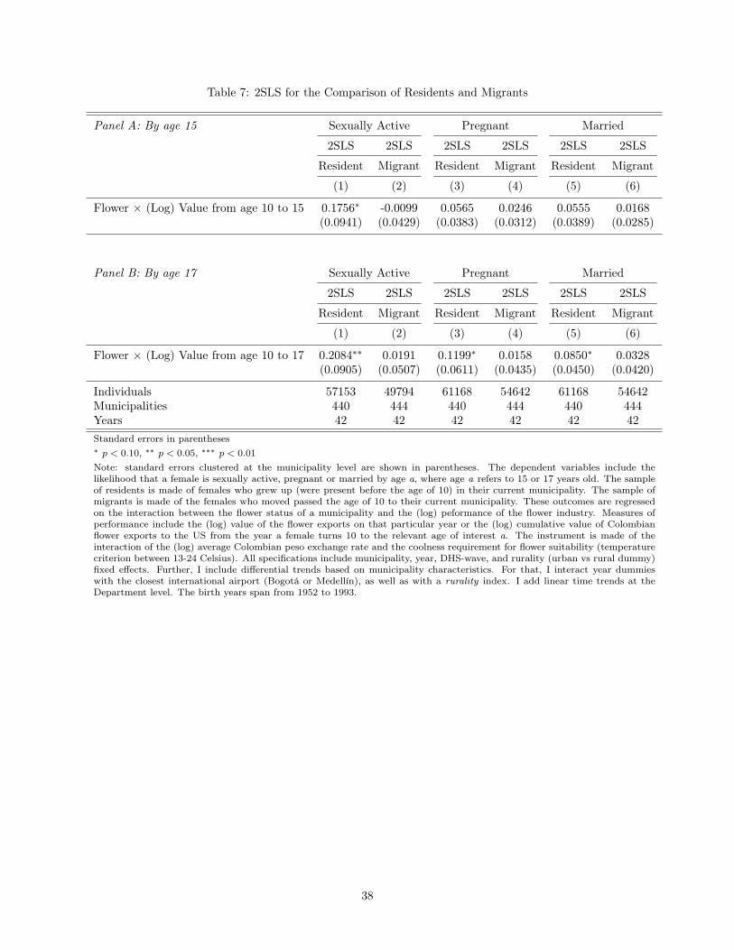
Table 7: 2SLS for the Comparison of Residents and Migrants

Panel A: By age 15 Sexually Active Pregnant Married

2SLS 2SLS 2SLS 2SLS 2SLS 2SLS

Resident Migrant Resident Migrant Resident Migrant

(1) (2) (3) (4) (5) (6)

Flower ⇥ (Log) Value from age 10 to 15 0.1756⇤ -0.0099 0.0565 0.0246 0.0555 0.0168(0.0941) (0.0429) (0.0383) (0.0312) (0.0389) (0.0285)

Panel B: By age 17 Sexually Active Pregnant Married

2SLS 2SLS 2SLS 2SLS 2SLS 2SLS

Resident Migrant Resident Migrant Resident Migrant

(1) (2) (3) (4) (5) (6)

Flower ⇥ (Log) Value from age 10 to 17 0.2084⇤⇤ 0.0191 0.1199⇤ 0.0158 0.0850⇤ 0.0328(0.0905) (0.0507) (0.0611) (0.0435) (0.0450) (0.0420)

Individuals 57153 49794 61168 54642 61168 54642Municipalities 440 444 440 444 440 444Years 42 42 42 42 42 42Standard errors in parentheses⇤p < 0.10, ⇤⇤

p < 0.05, ⇤⇤⇤p < 0.01

Note: standard errors clustered at the municipality level are shown in parentheses. The dependent variables include thelikelihood that a female is sexually active, pregnant or married by age a, where age a refers to 15 or 17 years old. The sampleof residents is made of females who grew up (were present before the age of 10) in their current municipality. The sample ofmigrants is made of the females who moved passed the age of 10 to their current municipality. These outcomes are regressedon the interaction between the flower status of a municipality and the (log) peformance of the flower industry. Measures ofperformance include the (log) value of the flower exports on that particular year or the (log) cumulative value of Colombianflower exports to the US from the year a female turns 10 to the relevant age of interest a. The instrument is made of theinteraction of the (log) average Colombian peso exchange rate and the coolness requirement for flower suitability (temperaturecriterion between 13-24 Celsius). All specifications include municipality, year, DHS-wave, and rurality (urban vs rural dummy)fixed effects. Further, I include differential trends based on municipality characteristics. For that, I interact year dummieswith the closest international airport (Bogotá or Medellín), as well as with a rurality index. I add linear time trends at theDepartment level. The birth years span from 1952 to 1993.

38

Table 8: 2SLS Results for Cundinamarca and Antioquia

Panel A: By age 15 Sexually Active Pregnant Married

2SLS 2SLS 2SLS 2SLS 2SLS 2SLS

(1) (2) (3) (4) (5) (6)

Flower ⇥ (Log) Value at age 15 0.0742⇤⇤⇤ 0.0354⇤ 0.0326⇤(0.0278) (0.0193) (0.0178)

Flower ⇥ (Log) Value from age 10 to 15 0.0607⇤⇤⇤ 0.0298⇤ 0.0281⇤(0.0230) (0.0156) (0.0149)

Panel B: By age 17 Sexually Active Pregnant Married

2SLS 2SLS 2SLS 2SLS 2SLS 2SLS

(1) (2) (3) (4) (5) (6)

Flower ⇥ (Log) Value at age 17 0.1191⇤⇤ 0.0862⇤⇤ 0.0684⇤⇤(0.0477) (0.0353) (0.0274)

Flower ⇥ (Log) Value from age 10 to 17 0.0964⇤⇤ 0.0725⇤⇤ 0.0565⇤⇤(0.0385) (0.0295) (0.0224)

Individuals 11369 11369 12905 12905 12905 12905Municipalities 101 101 101 101 101 101Years 42 42 42 42 42 42⇤p < 0.10, ⇤⇤

p < 0.05, ⇤⇤⇤p < 0.01

Note: standard errors clustered at the municipality level are shown in parentheses. The dependent variables include thelikelihood that a female is sexually active, pregnant or married by age a, where age a refers to 15 or 17 years old. Theseoutcomes are regressed on the interaction between the flower status of a municipality and the (log) peformance of the flowerindustry. Measures of performance include the (log) value of the flower exports on that particular year or the (log) cumulativevalue of Colombian flower exports to the US from the year a female turns 10 to the relevant age of interest a. The instrumentis made of the interaction of the (log) average Colombian peso exchange rate and the coolness requirement for flower suitability(temperature criterion between 13-24 Celsius). All specifications include municipality, year, DHS-wave, and rurality (urban vsrural dummy) fixed effects. Further, I include differential trends based on municipality characteristics. For that, I interact yeardummies with the closest international airport (Bogotá or Medellín), as well as with a rurality index. I add linear time trendsat the Department level. The sample is made of females who are between ages 17 and 50 on the survey year and report residingin the adminstrative departments of Cundinamarca or Antioquia. The birth years span from 1952 to 1993. Source: DHS waveof 1986, 1990, 1995, 2000, 2005 and 2010.

39

Appendix

Table A.1: Flower Suitability - All of Colombia

Flower Status Flower Hectares

(1) (2) (3) (4)

Coolness 0.192⇤⇤⇤ 14.597⇤⇤⇤(0.018) (3.100)

Hot -0.202⇤⇤⇤ -14.902⇤⇤⇤(0.018) (2.990)

Cold -0.156⇤⇤⇤ -8.751(0.039) (6.006)

Constant 0.026⇤⇤⇤ 0.218⇤⇤⇤ 0.704 14.976⇤⇤⇤(0.007) (0.017) (0.513) (2.990)

Municipalities 1086 1086 1086 1086R-Squared 0.080 0.085 0.017 0.017F-Stat 108.117 64.065 22.164 13.118⇤p < 0.10, ⇤⇤

p < 0.05, ⇤⇤⇤p < 0.01

Note: Note: robust standard errors reported in parentheses. OLS results toevaluate the suitability of a municipality for flower cultivation. The outcomevariables reflect both the extensive margin, flower status, as well as the in-tensive margin of cultivation, flower hectares. The flower status and flowerhectares are measured at the municipality level. The flower status identifieswhether a municipality is a flower-producing center or not. Hectares corre-sponds to the number of hectares under flower cultivation. The suitabilityrequirement exploits a discontinuity in temperature: coolness. It captureswhether the average annual temperature lies between 13-24 Celsius (55-75F), deemed to be optimal for flower growth. I add a dummy Hot for temper-atures that exceed 24 Celsius and a dummy Cold for temperatures that arebelow 13 Celsius as alternative suitable requirements. The sample consists ofall municipalities in Colombia (whether they were covered in the DHS surveysor not), for whic temperature is available.

40

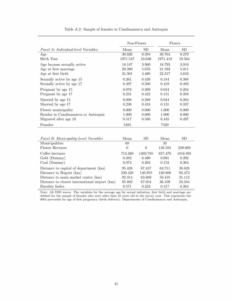
Table A.2: Sample of females in Cundinamarca and Antioquia

Non-Flower Flower

Panel A: Individual-level Variables Mean SD Mean SDAge 30.926 9.394 30.764 9.270Birth Year 1971.547 10.636 1971.418 10.564Age became sexually active 18.187 3.900 18.793 3.910Age at first marriage 20.380 5.076 21.593 5.011Age at first birth 21.301 4.460 22.317 4.616Sexually active by age 15 0.261 0.439 0.184 0.388Sexually active by age 17 0.497 0.500 0.419 0.493Pregnant by age 15 0.078 0.269 0.044 0.204Pregnant by age 17 0.231 0.422 0.151 0.358Married by age 15 0.098 0.298 0.044 0.204Married by age 17 0.236 0.424 0.131 0.337Flower municipality 0.000 0.000 1.000 0.000Resides in Cundinamarca or Antioquia 1.000 0.000 1.000 0.000Migrated after age 10 0.517 0.500 0.445 0.497Females 5485 7420

Panel B: Municipality-Level Variables Mean SD Mean SDMunicipalities 68 33Flower Hectares 0 0 138.585 229.669Coffee hectares 713.260 1403.785 657.470 1816.891Gold (Dummy) 0.382 0.490 0.091 0.292Coal (Dummy) 0.074 0.263 0.152 0.364Distance to capital of department (km) 95.438 67.457 63.711 38.628Distance to Bogotá (km) 230.428 140.955 120.806 92.473Distance to main market center (km) 92.314 63.869 50.418 31.112Distance to closest international airport (km) 95.802 67.054 36.109 23.584Rurality Index 0.571 0.233 0.417 0.264Note: All DHS waves. The variables for the average age for sexual initiation, first birth and marriage aredefined for the sample of females who were older than 25 years old in the survey year. This represents the90th percentile for age of first pregnancy (birth delivery). Departments of Cundinamarca and Antioquia.

41

Table A.3: 2SLS for Alternative Cumulative Exposures

Panel A: By age 15 Sexually Active Pregnant Married

2SLS 2SLS 2SLS 2SLS 2SLS 2SLS 2SLS 2SLS 2SLS

(1) (2) (3) (4) (5) (6) (7) (8) (9)

Flower ⇥ (Log) Value from 6 to 15 0.0718⇤⇤ 0.0354⇤ 0.0295(0.0361) (0.0208) (0.0198)

Flower ⇥ (Log) Value from 10 to 15 0.0713⇤⇤ 0.0356⇤ 0.0311(0.0360) (0.0210) (0.0207)

Flower ⇥ (Log) Value from 13 to 15 0.0667⇤⇤ 0.0334⇤ 0.0307(0.0337) (0.0195) (0.0202)

Panel B: By age 17 Sexually Active Pregnant Married

2SLS 2SLS 2SLS 2SLS 2SLS 2SLS 2SLS 2SLS 2SLS

(1) (2) (3) (4) (5) (6) (7) (8) (9)

Flower ⇥ (Log) Value from 6 to 17 0.0937⇤⇤ 0.0524⇤ 0.0501⇤(0.0446) (0.0316) (0.0294)

Flower ⇥ (Log) Value from 10 to 17 0.0984⇤⇤ 0.0546⇤ 0.0509⇤(0.0458) (0.0327) (0.0302)

Flower ⇥ (Log) Value from 13 to 17 0.1005⇤⇤ 0.0554⇤ 0.0497(0.0457) (0.0328) (0.0302)

Individuals 106966 106966 106966 115814 115814 115814 115814 115814 115814Municipalities 446 446 446 446 446 446 446 446 446Years 42 42 42 42 42 42 42 42 42⇤p < 0.10, ⇤⇤

p < 0.05, ⇤⇤⇤p < 0.01

Note: standard errors clustered at the municipality level are shown in parentheses. The dependent variables include the likelihood that a female is sexuallyactive, pregnant or married by age a, where age here refers to 15 or 17 years old. Measures of performance include the (log) cumulative value of Colombianflower exports to the US from the year a female turns 6, the year she turns 10 and the year she turns 13 to the relevant age of interest a. The instrument ismade of the interaction of the (log) average Colombian peso exchange rate and the coolness requirement for flower suitability (temperature criterion between13-24 Celsius). All specifications include municipality, year, DHS-wave, and rurality (urban vs rural dummy) fixed effects. Further, I include differentialtrends based on municipality characteristics. For that, I interact year dummies with the closest international airport (Bogotá or Medellín), as well as with arurality index. I add linear time trends at the Department level.

42

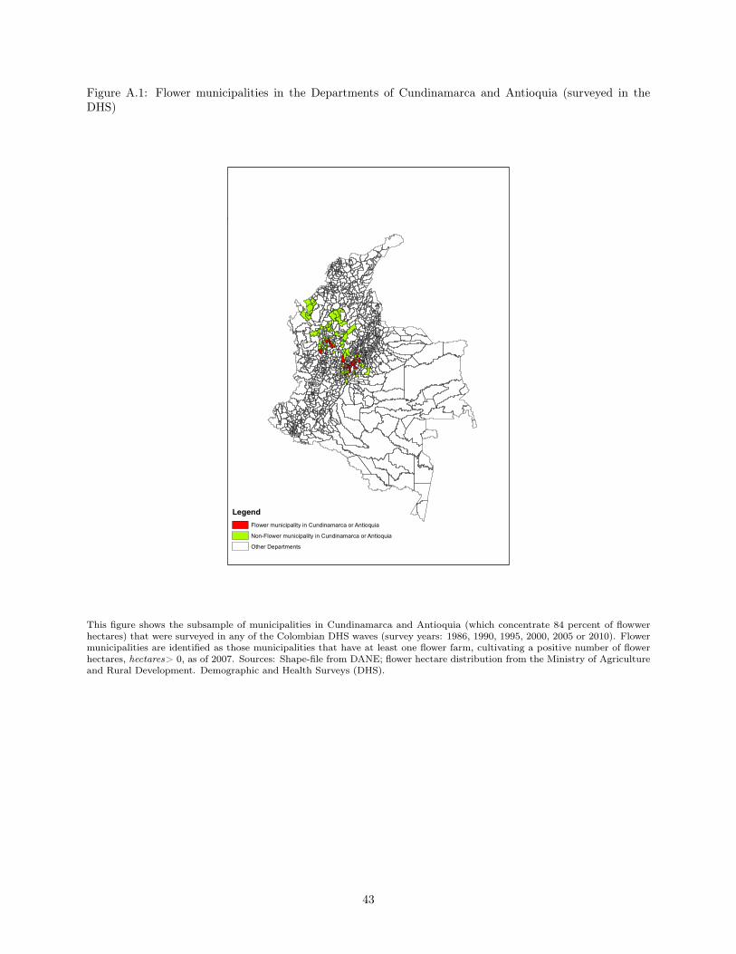
Figure A.1: Flower municipalities in the Departments of Cundinamarca and Antioquia (surveyed in theDHS)

LegendFlower municipality in Cundinamarca or Antioquia

Non-Flower municipality in Cundinamarca or Antioquia

Other Departments

This figure shows the subsample of municipalities in Cundinamarca and Antioquia (which concentrate 84 percent of flowwerhectares) that were surveyed in any of the Colombian DHS waves (survey years: 1986, 1990, 1995, 2000, 2005 or 2010). Flowermunicipalities are identified as those municipalities that have at least one flower farm, cultivating a positive number of flowerhectares, hectares> 0, as of 2007. Sources: Shape-file from DANE; flower hectare distribution from the Ministry of Agricultureand Rural Development. Demographic and Health Surveys (DHS).

43