Odds ratio, Odds ratio test for independence,

chi-squared statistic.

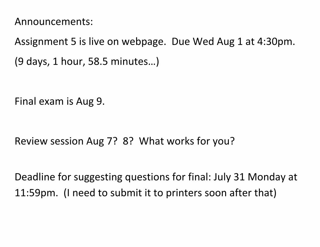
Announcements:

Assignment 5 is live on webpage. Due Wed Aug 1 at 4:30pm.

(9 days, 1 hour, 58.5 minutes…)

Final exam is Aug 9.

Review session Aug 7? 8? What works for you?

Deadline for suggesting questions for final: July 31 Monday at

11:59pm. (I need to submit it to printers soon after that)

Last time, we looked at odds, a modification of probability.

The odds of something happening is how many times more

likely the event happen is to something not happening.

Example: If the probability of something 0.6,

Then the odds of the effect are 0.6 / 0.4 = 3/2 or 1.5

That means the event is 1.5 times as likely as it not happening.

The formula for getting odds from probability P is:

Other equivalent interpretations:

Odds = Pr( Event) / Pr ( Not Event )

Odds = Pr( Success) / Pr ( Failure )

Example 1: If something is impossible, it has probability zero.

An impossible event has odds zero as well.

So an impossible event happening is zero times as likely as it

not happening.

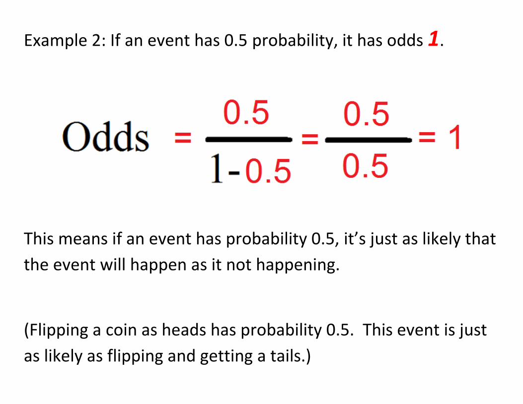
Example 2: If an event has 0.5 probability, it has odds 1.

This means if an event has probability 0.5, it’s just as likely that

the event will happen as it not happening.

(Flipping a coin as heads has probability 0.5. This event is just

as likely as flipping and getting a tails.)

Example 3: If something is certain to happen, it has probability

1. This event has odds infinity. (1 / 0)*

A certain event is infinitely more likely to occur than it not

happening.

These examples also provide the limits of odds. Odds are

always between 0 and infinity, and never negative.

for interest: You can get the probability from odds by using

… it’s handy to check your work.

for interest *: 1/0 should actually be 1 / 0+ to make it infinity

instead of undefined.

0+ means “zero, but always from the positive side”, which we

use because 1 – P is always positive because P is never above

1.

This is covered in calculus, so it’s here only for completion.

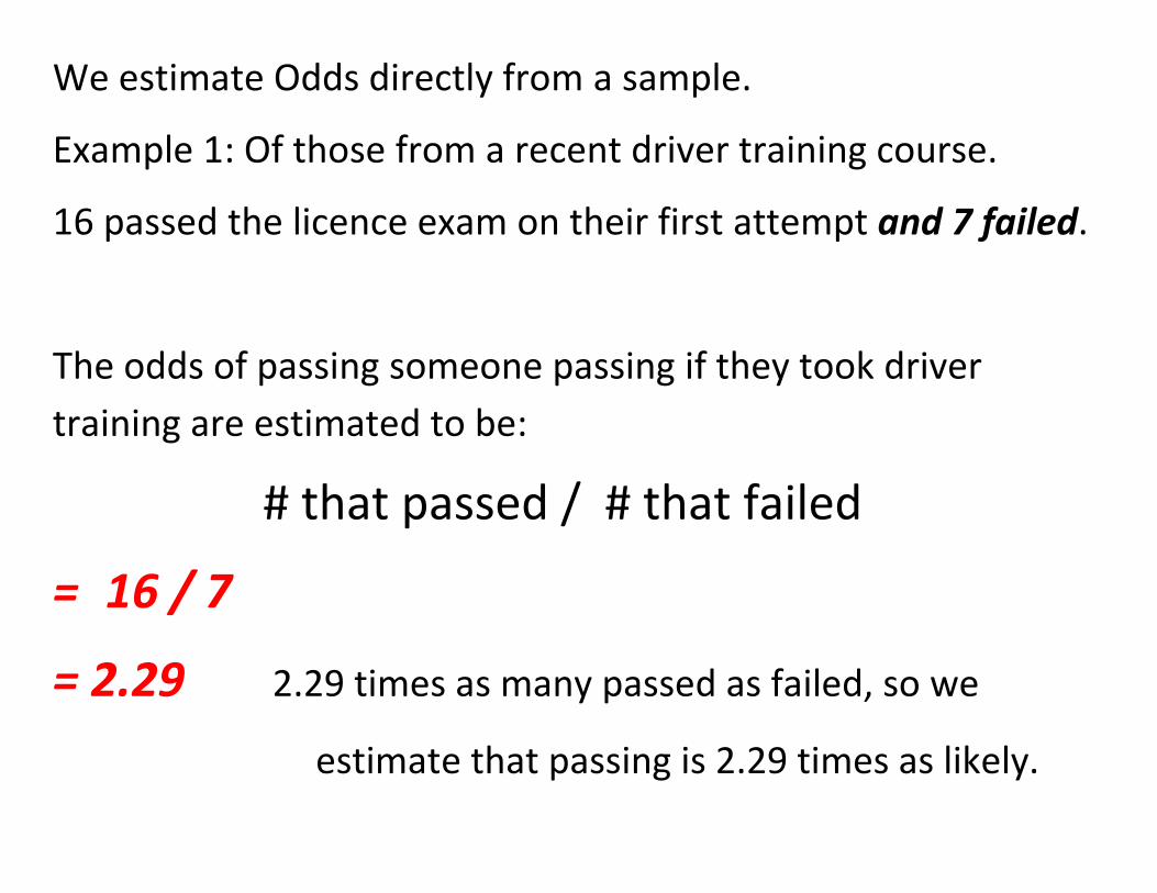
We estimate Odds directly from a sample.

Example 1: Of those from a recent driver training course.

16 passed the licence exam on their first attempt and 7 failed.

The odds of passing someone passing if they took driver

training are estimated to be:

# that passed / # that failed

= 16 / 7

= 2.29 2.29 times as many passed as failed, so we

estimate that passing is 2.29 times as likely.

Example 2: We also a sample of the exam results from those

that didn’t take the driver training.

8 of them passed their first time, and

11 of them failed.

The odds of passing without driver training are:

8 / 11, or 0.73 0.73 as many passed as failed, so passing is estimated to be

0.73 times as likely.

Sometimes it’s not odds, sometimes it’s just odd.

Odds ratio.

An odds ratio (OR) is a comparison between two odds.

The odds ratio, OR, shows which odds are larger and by how

much. Therefore, they also show which event is more likely,

and by how much.

It allows us to see if an event is more likely under certain

situations if we know the odds under each situation.

Example: The odds of passing the driving test with a course are

2.29. ( 16 / 7)

The odds of passing the test without a course are 0.73. (8 / 11)

The odds ratio of passing the test over taking the course are

This means that the odds of passing the test are 3.142 times as

large if you take a driver training course first.

This could be flipped to say that the odds of passing the test

are 0.318 times as large if don’t take driving training.

Quick formula for odds ratio

Odds Ratio = AD / BC

Multiply by these.

Divide by these.

Odds ratio = (11 x 16) / (7 x 8)

= 176 / 56 = 3.142

The odds of passing the test are 3.142 as large with a driver’s

course.

This way we don’t have to compute the odds beforehand.

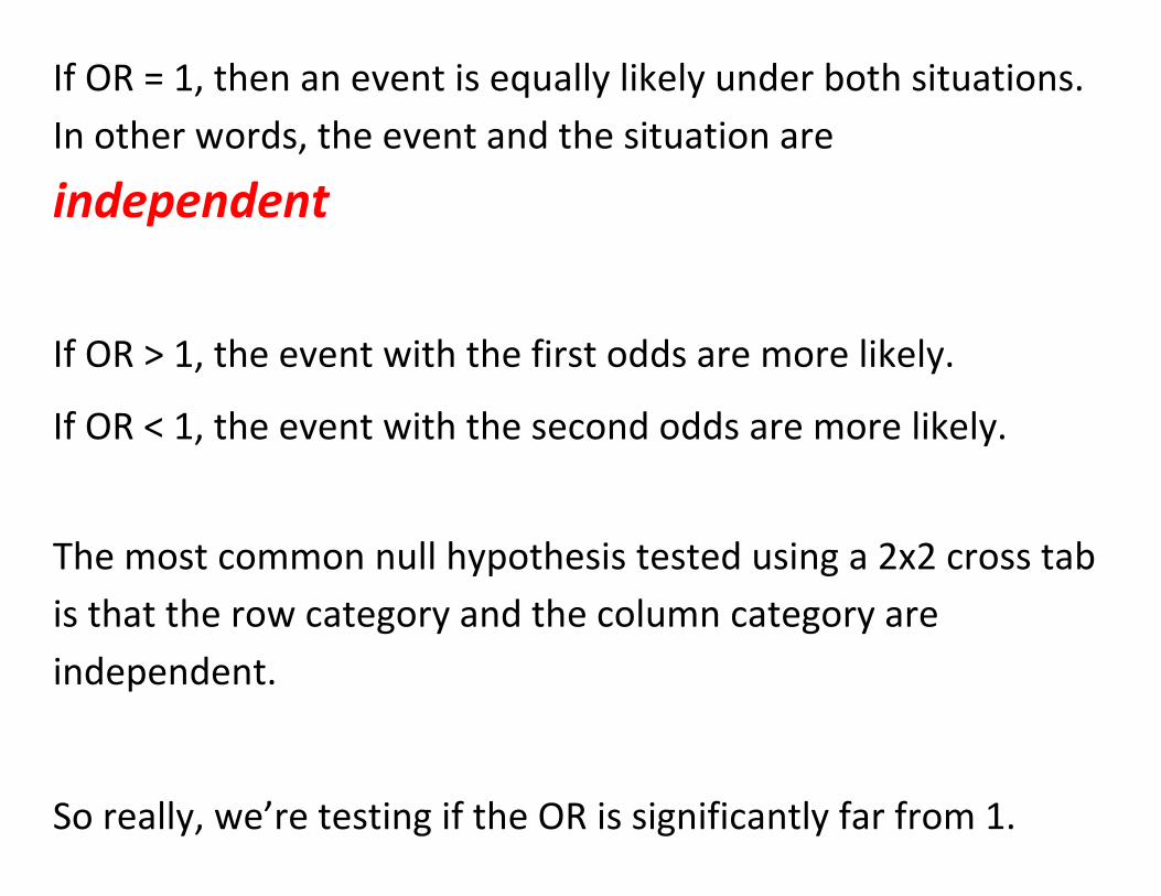
If OR = 1, then an event is equally likely under both situations.

In other words, the event and the situation are

independent

If OR > 1, the event with the first odds are more likely.

If OR < 1, the event with the second odds are more likely.

The most common null hypothesis tested using a 2x2 cross tab

is that the row category and the column category are

independent.

So really, we’re testing if the OR is significantly far from 1.

The odds ratio is 3.142. It’s above 1, but is it significantly so?

The 95% confidence interval of the odds ratio is:

(0.881 to 11.215) , which includes 1.

So OR = 1 is in the interval, we fail to reject the hypothesis

that these pass the test and taking the class are independent.

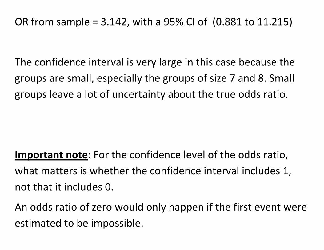
OR from sample = 3.142, with a 95% CI of (0.881 to 11.215)

The confidence interval is very large in this case because the

groups are small, especially the groups of size 7 and 8. Small

groups leave a lot of uncertainty about the true odds ratio.

Important note: For the confidence level of the odds ratio,

what matters is whether the confidence interval includes 1,

not that it includes 0.

An odds ratio of zero would only happen if the first event were

estimated to be impossible.

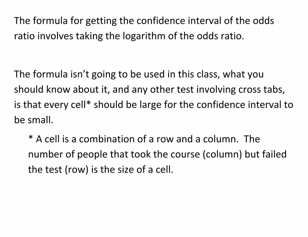
The formula for getting the confidence interval of the odds

ratio involves taking the logarithm of the odds ratio.

The formula isn’t going to be used in this class, what you

should know about it, and any other test involving cross tabs,

is that every cell* should be large for the confidence interval to

be small.

* A cell is a combination of a row and a column. The

number of people that took the course (column) but failed

the test (row) is the size of a cell.

SPSS: Computing odds ratio and its confidence interval.

First, recall how to build a crosstab.

Analyze Descriptive Stats Crosstabs

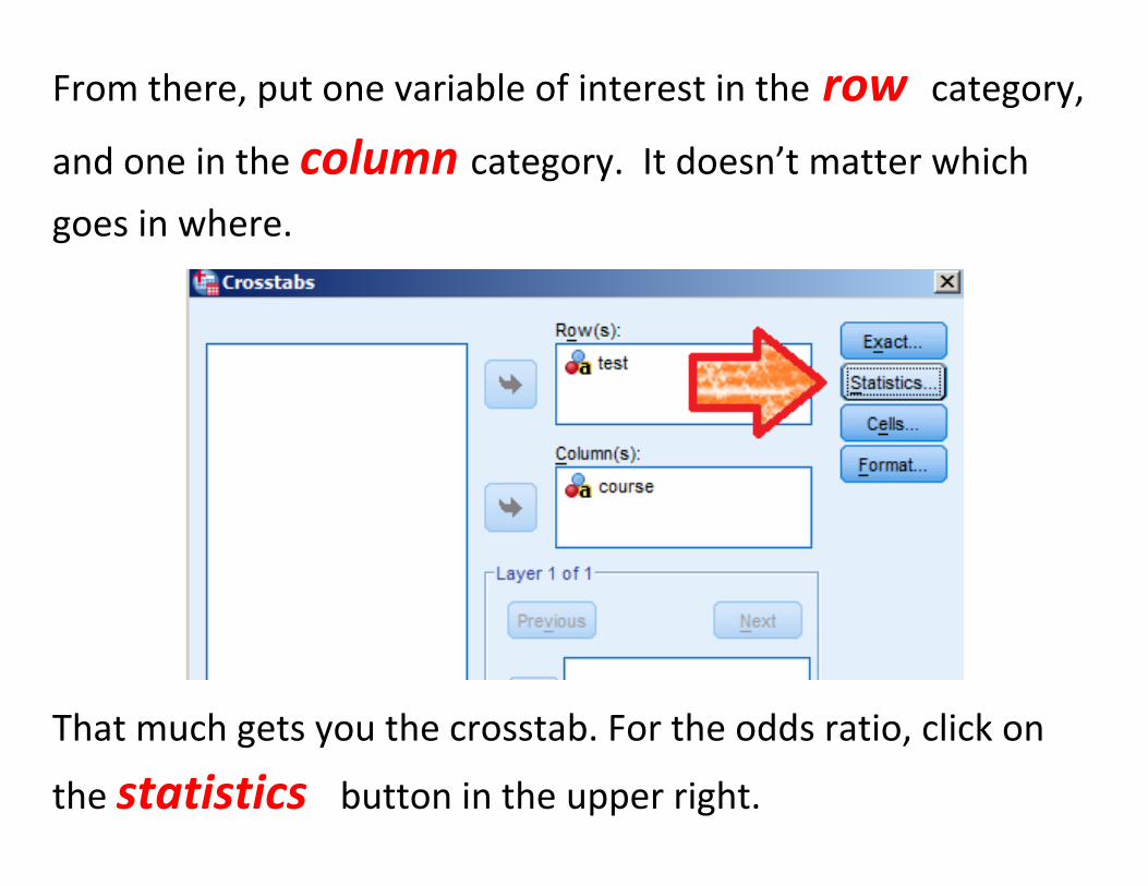
From there, put one variable of interest in the row category,

and one in the column category. It doesn’t matter which

goes in where.

That much gets you the crosstab. For the odds ratio, click on

the statistics button in the upper right.

To get the odds ratio, check off risk.

It’s under “risk” because odds ratio is related to relative risk.

Click “Continue”, then “Okay”.

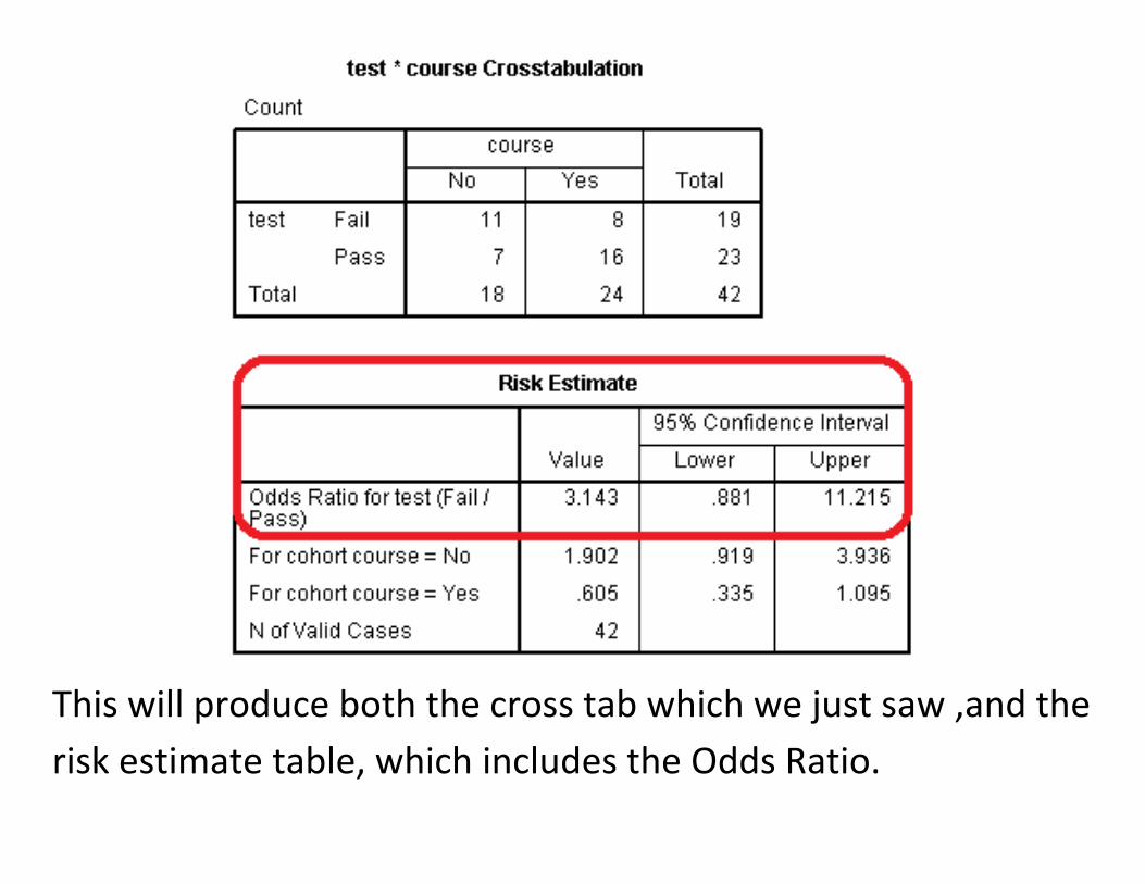
This will produce both the cross tab which we just saw ,and the

risk estimate table, which includes the Odds Ratio.

Unlike other confidence intervals that we’ve seen where the

estimated value is in the middle of the confidence interval, the

odds ratio appears closer to the lower side.

CI from odds ratio isn’t just a + or - like the other ones, the

odds ratio is being X and / by a some amount to get these

values.

Eyelash Crested Geckos. Good pets, but their bodies have the

consistency of uncooked chicken strips.

Odds ratios are only useful for testing for independence in a

2x2 contingency square.

You can also make the odds ratio a one-sided test at half the

alpha of the two-sided confidence interval.

If both ends of the 95% confidence interval in the driver testing

problem were positive, we could have concluded at the 0.025

level that getting driving training didn’t change the odds of

passing the test, it improved them.

The χ2 , or chi-squared (pronounced ky squared) test for

independence is useful for 2x3, 4x2, 5x5 cross tabs, or cross

tabs of any number of row or columns.

However, the only thing it checks for is independence.

So you can’t tell if the odds in a particular situation are more

than in another situation, only that there is a difference.

To understand the χ2 statistic, we first need to know about

expected values.

Expected frequencies are the number of responses in each cell

you would expect under the null assumption of independence.

To illusrate, say we found 40 people that like bearded dragons

and 40 people that didn’t, and tested to see if they were

clinically insane.

Our observed frequencies might look like:

OBSERVED Likes Dragons Dislikes Dragons Sane 37 33 Insane 3 7

OBSERVED Likes Dragons Dislikes Dragons Total Sane 37 33 70 Insane 3 7 10 Total 40 40 80

From the totals, 70 of 80, or 7/8 of the people we tested were

sane.

If liking dragons and being sane were independent, we would

expect that 7/8 of the people in each group would be sane.

In other words, we’d expect the same proportion of people in

each group to be sane or insane regard of dragon liking status.

Each like/dislike group has 40 people, and 7/8 of 40 is 35, so

the expected frequencies would be:

EXPECTED Likes Dragons Dislikes Dragons Total Sane 35 35 70 Insane 5 5 10 Total 40 40 80

Note that totals are the same as with the observed

frequencies, but now the cells are evened out.

The OR would be: (35 x 5) / (35 x 5) = 1, showing

independence.

The expected frequencies are calculated from the totals.

So the expected number of sane dragon likers would be…

…because there are 40 dragon likers, 70 sane people, and 80

people in total.

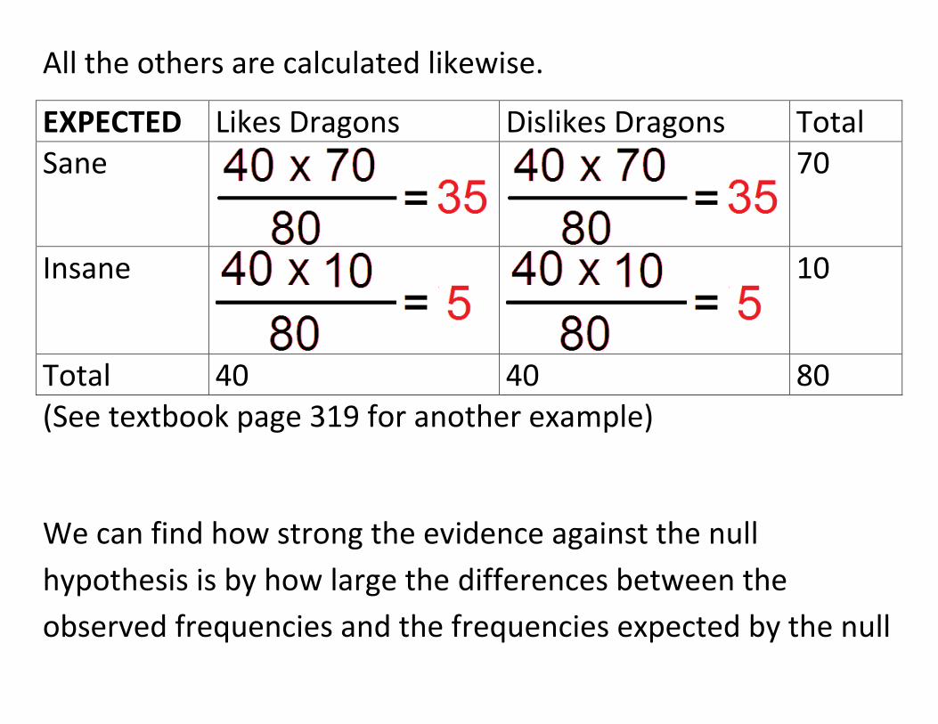
All the others are calculated likewise.

EXPECTED Likes Dragons Dislikes Dragons Total Sane

70

Insane

10

Total 40 40 80 (See textbook page 319 for another example)

We can find how strong the evidence against the null

hypothesis is by how large the differences between the

observed frequencies and the frequencies expected by the null

DIFFERENCES OBS - EXP

Likes Dragons Dislikes Dragons

Sane 37 - 35 33 - 35 Insane 5 - 7 5 - 3

Or, calculating…

DIFFERENCES OBS - EXP

Likes Dragons Dislikes Dragons

Sane 2 -2 Insane -2 2

If the differences in sanity levels was larger…

OBSERVED Likes Dragons Dislikes Dragons Sane 37 23 Insane 3 17

The differences between the observed and expected values

would become larger as well.

DIFFERENCES OBS - EXP

Likes Dragons Dislikes Dragons

Sane 7 -7 Insane -7 7

The χ2 statistic gets larger when the differences between

the expected and the observed get larger.

Σ means “add up all the..” whatever is to the right of it.

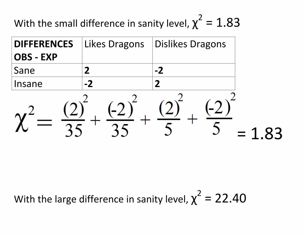
With the small difference in sanity level, χ2 = 1.83

DIFFERENCES OBS - EXP

Likes Dragons Dislikes Dragons

Sane 2 -2 Insane -2 2

= 1.83

With the large difference in sanity level, χ2 = 22.40

The χ2 statistic, like the t-statistic, is compared to a table of

critical values in the back of your book, page 523 (or in the

table that was sent out with assignment 5).

The degrees of freedom for a cross tab are

(rows – 1) x (columns – 1)

So in a 2x2 cross tab as we have, we’d only have

(2 – 1) x ( 2- 1 ) = 1 degree of freedom.

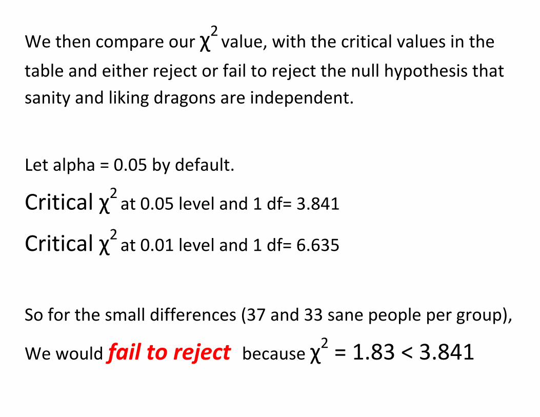
We then compare our χ2 value, with the critical values in the

table and either reject or fail to reject the null hypothesis that

sanity and liking dragons are independent.

Let alpha = 0.05 by default.

Critical χ2 at 0.05 level and 1 df= 3.841

Critical χ2 at 0.01 level and 1 df= 6.635

So for the small differences (37 and 33 sane people per group),

We would fail to reject because χ2 = 1.83 < 3.841

Next time: Getting expected values and chi-squared stats from

SPSS. Lots of examples.