October 31, 2005Copyright © 2001-5 by Erik D. Demaine and Charles E. LeisersonL13.1 Introduction to...
42
October 31, 2005 Copyright © 2001-5 by Erik D. Demaine and Charles E. Leiserson L13.1 Introduction to Algorithms LECTURE 11 Amortized Analysis • Dynamic tables • Aggregate method • Accounting method • Potential method
-
Upload
riley-simpson -
Category
Documents
-
view
214 -
download
0
Transcript of October 31, 2005Copyright © 2001-5 by Erik D. Demaine and Charles E. LeisersonL13.1 Introduction to...

October 31, 2005 Copyright © 2001-5 by Erik D. Demaine and Charles E. Leiserson L13.1
Introduction to Algorithms
LECTURE 11Amortized Analysis• Dynamic tables• Aggregate method• Accounting method• Potential method

October 31, 2005 Copyright © 2001-5 by Erik D. Demaine and Charles E. Leiserson L13.2
How large should a hash table be?
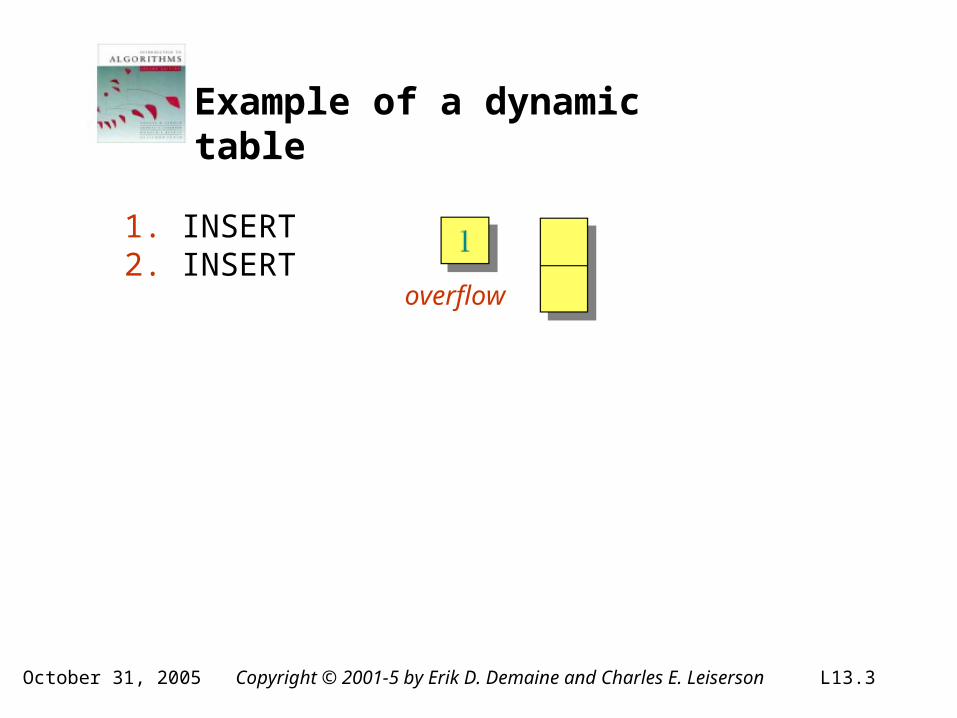
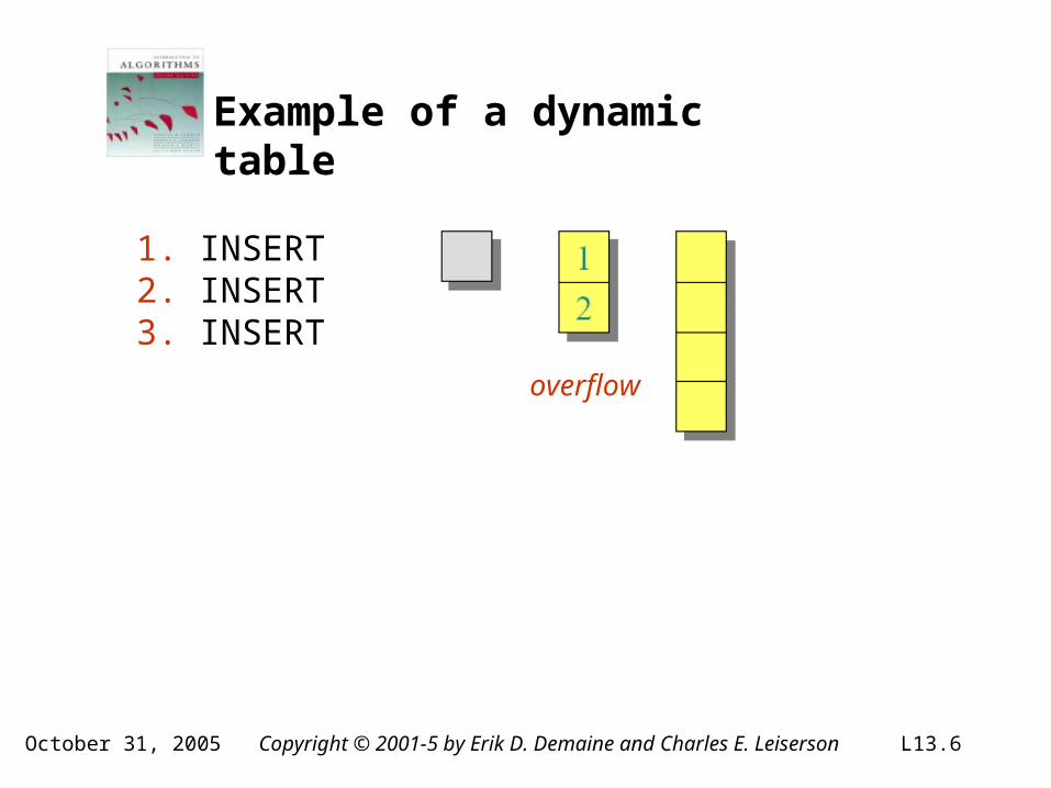
Goal: Make the table as small as possible, but large enough so that it won’t overflow (or otherwise become inefficient). Problem: What if we don’t know the proper sizein advance? Solution:Dynamic tables.IDEA: Whenever the table overflows, “grow” it by allocating (via malloc or new) a new, largertable. Move all items from the old table into the new one, and free the storage for the old table.
October 31, 2005 Copyright © 2001-5 by Erik D. Demaine and Charles E. Leiserson L13.3
Example of a dynamic table
1. INSERT2. INSERT
overflow

October 31, 2005 Copyright © 2001-5 by Erik D. Demaine and Charles E. Leiserson L13.4
Example of a dynamic table
1. INSERT2. INSERT
overflow

October 31, 2005 Copyright © 2001-5 by Erik D. Demaine and Charles E. Leiserson L13.5
Example of a dynamic table
1. INSERT2. INSERT
October 31, 2005 Copyright © 2001-5 by Erik D. Demaine and Charles E. Leiserson L13.6
Example of a dynamic table
1. INSERT2. INSERT3. INSERT
overflow

October 31, 2005 Copyright © 2001-5 by Erik D. Demaine and Charles E. Leiserson L13.7
Example of a dynamic table
1. INSERT2. INSERT3. INSERT
overflow

October 31, 2005 Copyright © 2001-5 by Erik D. Demaine and Charles E. Leiserson L13.8
Example of a dynamic table
1. INSERT2. INSERT3. INSERT

October 31, 2005 Copyright © 2001-5 by Erik D. Demaine and Charles E. Leiserson L13.9
Example of a dynamic table
1. INSERT2. INSERT3. INSERT4. INSERT

October 31, 2005 Copyright © 2001-5 by Erik D. Demaine and Charles E. Leiserson L13.10
Example of a dynamic table
1. INSERT2. INSERT3. INSERT4. INSERT5. INSERT
overflow

October 31, 2005 Copyright © 2001-5 by Erik D. Demaine and Charles E. Leiserson L13.11
Example of a dynamic table
1. INSERT2. INSERT3. INSERT4. INSERT5. INSERT
overflow

October 31, 2005 Copyright © 2001-5 by Erik D. Demaine and Charles E. Leiserson L13.12
Example of a dynamic table
1. INSERT2. INSERT3. INSERT4. INSERT5. INSERT

October 31, 2005 Copyright © 2001-5 by Erik D. Demaine and Charles E. Leiserson L13.13
Example of a dynamic table
1. INSERT2. INSERT3. INSERT4. INSERT5. INSERT6. INSERT7. INSERT

October 31, 2005 Copyright © 2001-5 by Erik D. Demaine and Charles E. Leiserson L13.14
Worst-case analysis
Consider a sequence of n insertions. The worst-case time to execute one insertion is Θ(n). Therefore, the worst-case time for n insertions is n·Θ(n) = Θ(n2).
WRONG! In fact, the worst-case cost for n insertions is only Θ(n) Θ(≪ n2).
Let’s see why.

October 31, 2005 Copyright © 2001-5 by Erik D. Demaine and Charles E. Leiserson L13.15
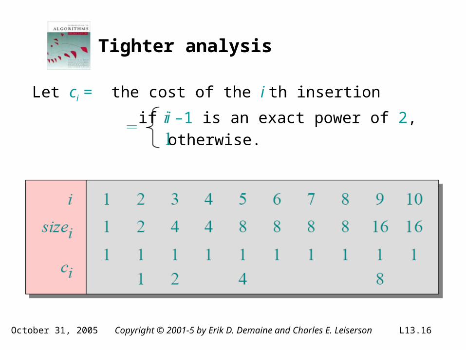
Tighter analysis
Let ci = the cost of the i th insertion
if i –1 is an exact power of 2,
otherwise.
October 31, 2005 Copyright © 2001-5 by Erik D. Demaine and Charles E. Leiserson L13.16
Tighter analysis
Let ci = the cost of the i th insertion
if i –1 is an exact power of 2,
otherwise.

October 31, 2005 Copyright © 2001-5 by Erik D. Demaine and Charles E. Leiserson L13.17
Tighter analysis (continued)
Cost of n insertions.
Thus, the average cost of each dynamic-table operation is Θ(n)/n= Θ(1).
October 31, 2005 Copyright © 2001-5 by Erik D. Demaine and Charles E. Leiserson L13.18
Amortized analysis
An amortized analysis is any strategy for analyzing a sequence of operations to show that the average cost per operation is small, even though a single operation within the sequence might be expensive.
Even though we’re taking averages, however, probability is not involved!
• An amortized analysis guarantees the average performance of each operation in the worst case.

October 31, 2005 Copyright © 2001-5 by Erik D. Demaine and Charles E. Leiserson L13.19
Types of amortized analyses
Three common amortization arguments:• the aggregate method,• the accounting method,• the potential method.
We’ve just seen an aggregate analysis.
The aggregate method, though simple, lacks the precision of the other two methods. In particular, the accounting and potential methods allow a specific amortized cost to be allocated to each operation.

October 31, 2005 Copyright © 2001-5 by Erik D. Demaine and Charles E. Leiserson L13.20
Accounting method
• Charge i th operation a fictitious amortized cost ĉi , where $1 pays for 1 unit of work (i.e., time).• This fee is consumed to perform the operation.• Any amount not immediately consumed is stored in the bank for use by subsequent operations.• The bank balance must not go negative! We must ensure that
for all n.• Thus, the total amortized costs provide an upper bound on the total true costs.
October 31, 2005 Copyright © 2001-5 by Erik D. Demaine and Charles E. Leiserson L13.21
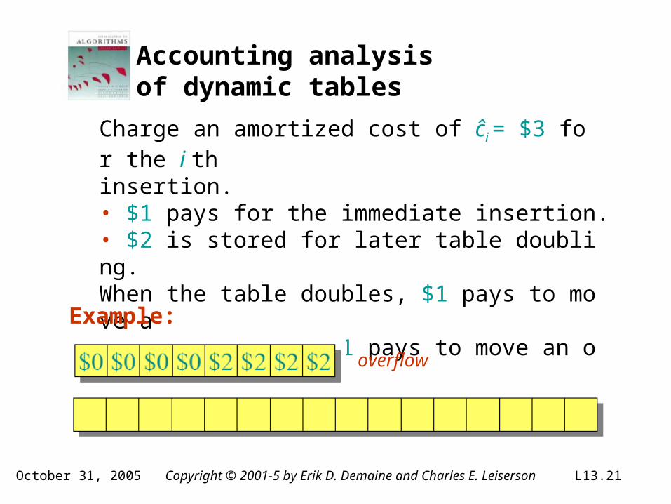
Accounting analysis of dynamic tables
Charge an amortized cost of ĉi = $3 for the i thinsertion.• $1 pays for the immediate insertion.• $2 is stored for later table doubling.When the table doubles, $1 pays to move a recent item, and $1 pays to move an old item.
Example:
overflow
October 31, 2005 Copyright © 2001-5 by Erik D. Demaine and Charles E. Leiserson L13.22
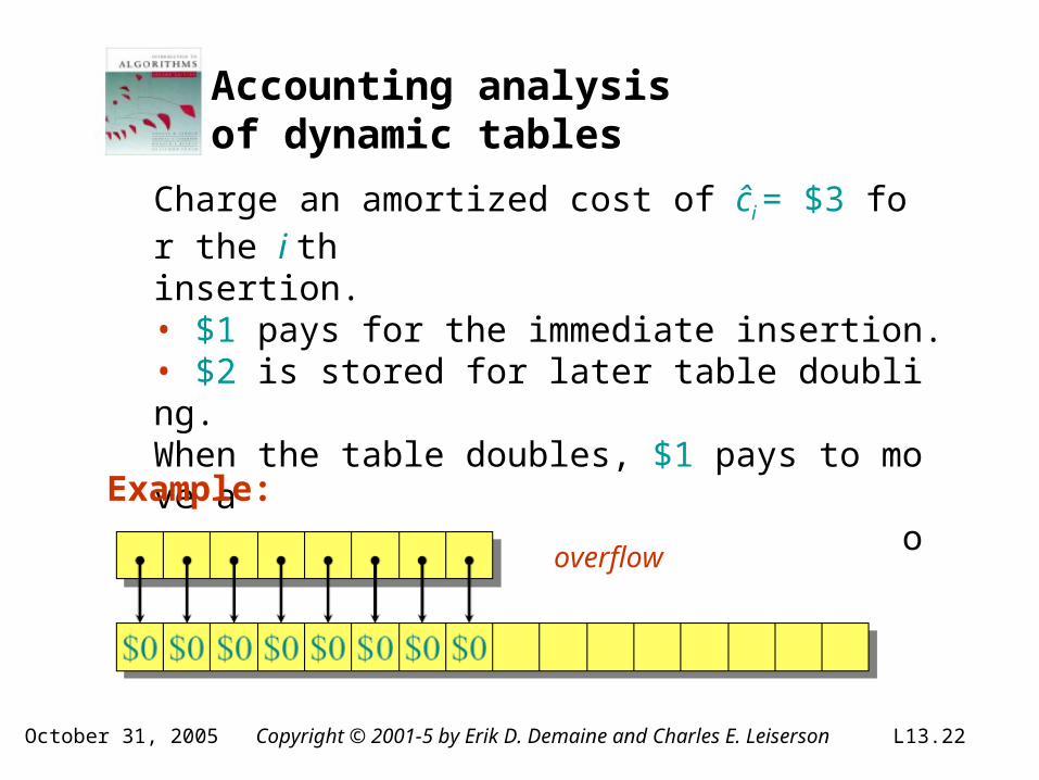
Accounting analysis of dynamic tables
Charge an amortized cost of ĉi = $3 for the i thinsertion.• $1 pays for the immediate insertion.• $2 is stored for later table doubling.When the table doubles, $1 pays to move a recent item, and $1 pays to move an old item.
Example:
overflow

October 31, 2005 Copyright © 2001-5 by Erik D. Demaine and Charles E. Leiserson L13.23
Accounting analysis of dynamic tables
Charge an amortized cost of ĉi = $3 for the i thinsertion.• $1 pays for the immediate insertion.• $2 is stored for later table doubling.When the table doubles, $1 pays to move a recent item, and $1 pays to move an old item.
Example:

October 31, 2005 Copyright © 2001-5 by Erik D. Demaine and Charles E. Leiserson L13.24
Accounting analysis (continued)
Key invariant: Bank balance never drops below 0. Thus, the sum of the amortized costs provides an upper bound on the sum of the true costs.
*Okay, so I lied. The first operation costs only $2, not $3.
October 31, 2005 Copyright © 2001-5 by Erik D. Demaine and Charles E. Leiserson L13.25
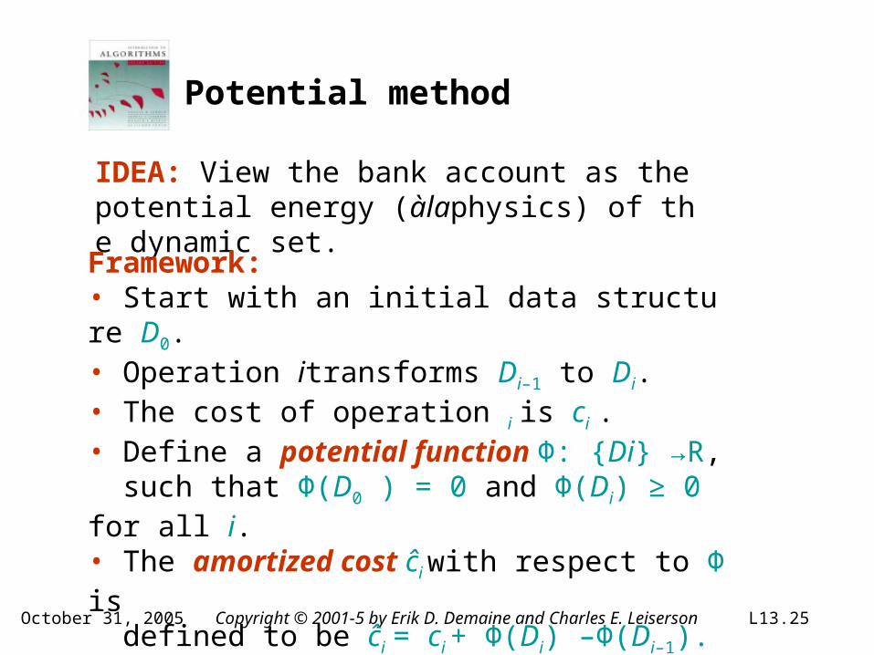
Potential method
IDEA: View the bank account as the potential energy (àlaphysics) of the dynamic set.
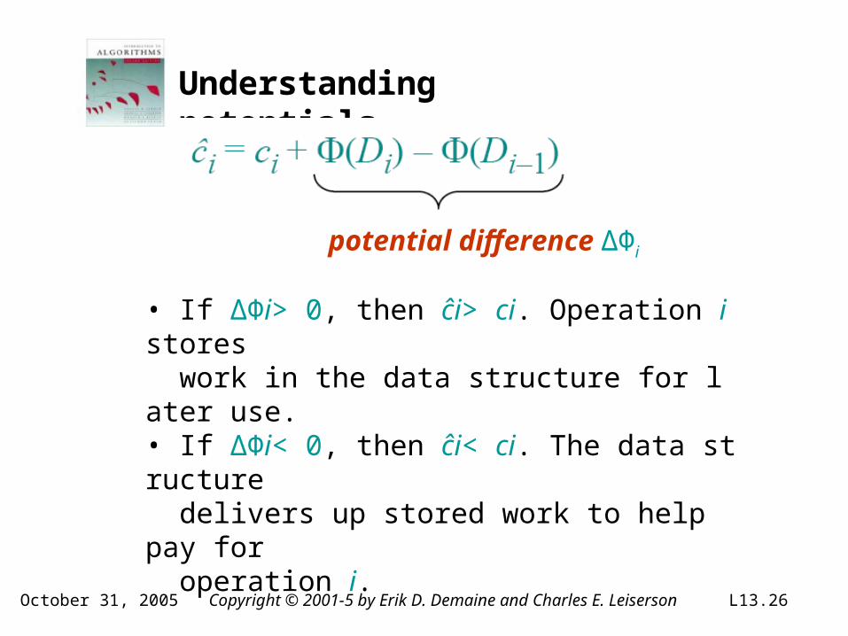
Framework:• Start with an initial data structure D0.• Operation itransforms Di–1 to Di. • The cost of operation i is ci .• Define a potential function Φ: {Di} →R, such that Φ(D0 ) = 0 and Φ(Di) ≥ 0 for all i. • The amortized cost ĉi with respect to Φ is defined to be ĉi = ci + Φ(Di) –Φ(Di–1).
October 31, 2005 Copyright © 2001-5 by Erik D. Demaine and Charles E. Leiserson L13.26
Understanding potentials
potential difference ΔΦi
• If ΔΦi> 0, then ĉi> ci. Operation i stores work in the data structure for later use.• If ΔΦi< 0, then ĉi< ci. The data structure delivers up stored work to help pay for operation i.
October 31, 2005 Copyright © 2001-5 by Erik D. Demaine and Charles E. Leiserson L13.27
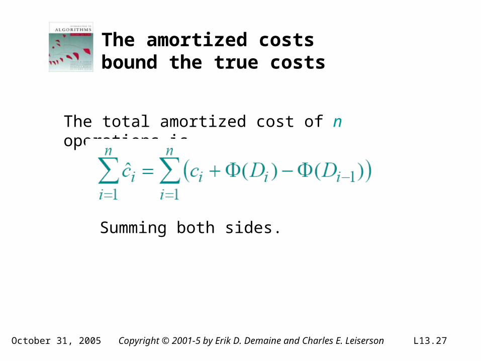
The amortized costs bound the true costs
The total amortized cost of n operations is
Summing both sides.

October 31, 2005 Copyright © 2001-5 by Erik D. Demaine and Charles E. Leiserson L13.28
The amortized costs bound the true costs
The total amortized cost of n operations is
The series telescopes.

October 31, 2005 Copyright © 2001-5 by Erik D. Demaine and Charles E. Leiserson L13.29
The amortized costs bound the true costs
The total amortized cost of n operations is

October 31, 2005 Copyright © 2001-5 by Erik D. Demaine and Charles E. Leiserson L13.30
Potential analysis of table doubling
Define the potential of the table after the ith insertion by (Assume that
Note:
Example:
accounting method )

October 31, 2005 Copyright © 2001-5 by Erik D. Demaine and Charles E. Leiserson L13.31
Calculation of amortized costs
The amortized cost of the i th insertion is

October 31, 2005 Copyright © 2001-5 by Erik D. Demaine and Charles E. Leiserson L13.32
Calculation of amortized costs
The amortized cost of the i th insertion is
if i –1is an exact power of 2,
otherwise;
October 31, 2005 Copyright © 2001-5 by Erik D. Demaine and Charles E. Leiserson L13.33
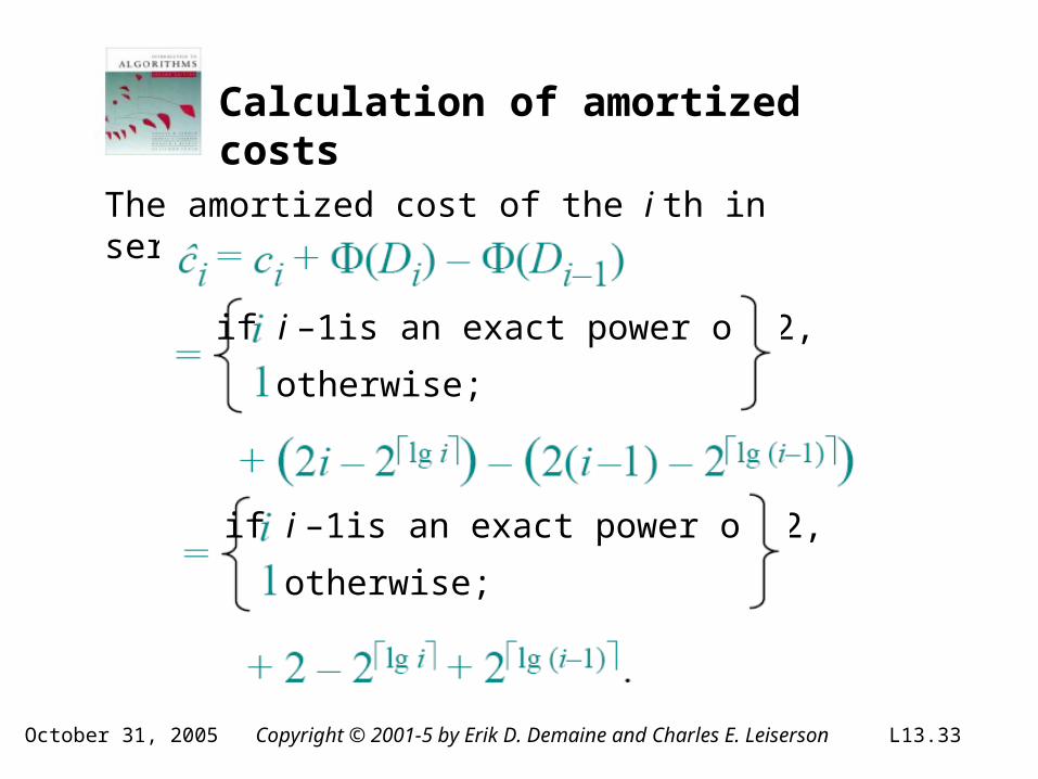
Calculation of amortized costs
The amortized cost of the i th insertion is
if i –1is an exact power of 2,
otherwise;
if i –1is an exact power of 2,
otherwise;

October 31, 2005 Copyright © 2001-5 by Erik D. Demaine and Charles E. Leiserson L13.34
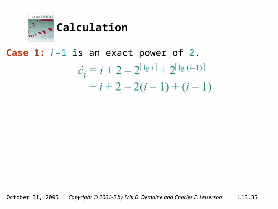
Calculation
Case 1: i –1 is an exact power of 2.
October 31, 2005 Copyright © 2001-5 by Erik D. Demaine and Charles E. Leiserson L13.35
Calculation
Case 1: i –1 is an exact power of 2.

October 31, 2005 Copyright © 2001-5 by Erik D. Demaine and Charles E. Leiserson L13.36
Calculation
Case 1: i –1 is an exact power of 2.

October 31, 2005 Copyright © 2001-5 by Erik D. Demaine and Charles E. Leiserson L13.37
Calculation
Case 1: i –1 is an exact power of 2.

October 31, 2005 Copyright © 2001-5 by Erik D. Demaine and Charles E. Leiserson L13.38
Calculation
Case 1: i –1 is an exact power of 2.
Case 2: i –1 is not an exact power of 2.

October 31, 2005 Copyright © 2001-5 by Erik D. Demaine and Charles E. Leiserson L13.39
Calculation
Case 1: i –1 is an exact power of 2.
Case 2: i –1 is not an exact power of 2.

October 31, 2005 Copyright © 2001-5 by Erik D. Demaine and Charles E. Leiserson L13.40
Calculation
Case 1: i –1 is an exact power of 2.
Case 2: i –1 is not an exact power of 2.
Therefore, n insertions cost Θ(n) in the worst case.

October 31, 2005 Copyright © 2001-5 by Erik D. Demaine and Charles E. Leiserson L13.41
Calculation
Case 1: i –1 is an exact power of 2.
Case 2: i –1 is not an exact power of 2.
Therefore, n insertions cost Θ(n) in the worst case.Exercise: Fix the bug in this analysis to show that the amortized cost of the first insertion is only 2.
October 31, 2005 Copyright © 2001-5 by Erik D. Demaine and Charles E. Leiserson L13.42
Conclusions
• Amortized costs can provide a clean abstraction of data-structure performance.• Any of the analysis methods can be used when an amortized analysis is called for, but each method has some situations where it is arguably the simplest or most precise.• Different schemes may work for assigning amortized costs in the accounting method, or potentials in the potential method, sometimes yielding radically different bounds.