CITATION

Jensen, T.G., H.W. Wijesekera, E.S. Nyadjro, P.G. Thoppil, J.F. Shriver, K.K. Sandeep,

and V. Pant. 2016. Modeling salinity exchanges between the equatorial Indian Ocean

and the Bay of Bengal. Oceanography 29(2):92–101, http://dx.doi.org/10.5670/

oceanog.2016.42.

DOI

http://dx.doi.org/10.5670/oceanog.2016.42

COPYRIGHT

This article has been published in Oceanography, Volume 29, Number 2, a quarterly

journal of The Oceanography Society. Copyright 2016 by The Oceanography Society.

All rights reserved.

USAGE

Permission is granted to copy this article for use in teaching and research.

Republication, systematic reproduction, or collective redistribution of any portion of

this article by photocopy machine, reposting, or other means is permitted only with the

approval of The Oceanography Society. Send all correspondence to: info@tos.org or

The Oceanography Society, PO Box 1931, Rockville, MD 20849-1931, USA.

OceanographyTHE OFFICIAL MAGAZINE OF THE OCEANOGRAPHY SOCIETY

DOWNLOADED FROM HTTP://TOS.ORG/OCEANOGRAPHY

Oceanography | Vol.29, No.292

BAY OF BENGAL: FROM MONSOONS TO MIXING

ABSTRACT. With a focus on the Bay of Bengal, models ranging from a 1/12.5° global ocean model to a ¼° regional Indian Ocean model to a 2 km local high-resolution coupled model are used to simulate salinity exchanges in the Indian Ocean. Global Hybrid Coordinate Ocean Model simulations show a surprisingly large persistent flow of high-salinity water from the equatorial Indian Ocean into the Bay of Bengal during the northeast monsoon, although it is weaker than during the southwest monsoon. On average, salt is transported into the Bay of Bengal between 83°E and 95°E, and low-salinity water flows southward near the east coast of Sri Lanka and east of 95°E. The Regional Ocean Modeling System shows that knowledge of river input of freshwater is essential for modeling surface salinities correctly in the Bay of Bengal. High-resolution coupled model simulations are in agreement with recent observations and show that a strong subsurface current with a speed of about 1 m s–1 intrudes into the Bay of Bengal beneath southward-flowing low-salinity water during the northeast monsoon. The subsurface high-salinity water, which originates in the northern Arabian Sea,

spreads northward into the Bay of Bengal and downward along constant density surfaces. North of 10°N, the model simulation implies that mixing takes place on density surfaces at depths of 100–150 m after advection of cold, low-salinity water from the north, and subsequent stirring of the two water masses. Vertical diffusion plays an insignificant role in this mixing.

Modeling Salinity Exchanges Between the Equatorial Indian Ocean

and the Bay of Bengal

By Tommy G. Jensen,

Hemantha W. Wijesekera,

Ebenezer S. Nyadjro,

Prasad G. Thoppil,

Jay F. Shriver,

K.K. Sandeep,

and Vimlesh Pant

Oceanography | Vol.29, No.292

Oceanography | June 2016 93

equatorial Rossby waves that propagate only along the equator in the so-called equatorial wave guide (Matsuno, 1966). They play a vital role in the onset of the El Niño-Southern Oscillation in the Pacific, and are thought to play a key role in intraseasonal oscillations in the Indian Ocean. The latter is an important link in the global circulation as it connects the Pacific Ocean to the Indian Ocean via the Indonesian Throughflow (e.g., Qiu et al., 1999; Shinoda et al., 2012).

The Indian Ocean basin is only about 5,000 km wide, and the fast equato-rial Kelvin waves and equatorial Rossby waves combine to produce a strong reso-nant 180-day periodic response (Jensen, 1993) and significant periodic responses on 90-day and shorter intraseasonal time scales (Han, 2005). Variability in currents and sea level on those time scales is there-fore common in the equatorial region that links the Bay of Bengal with the Arabian Sea and impacts both of them. The influ-ence of equatorial waves on the Bay of Bengal is well documented in mod-els (e.g., Yu et al., 1991; McCreary et al., 1996). These models show that coastally trapped Kelvin waves are generated when equatorial Kelvin waves reflect off the island of Sumatra. As these waves prop-agate northward into the Bay of Bengal, they excite long westward-propagating Rossby waves that affect the bay’s interior.

South of the equator, annual Rossby

waves emerging from Northwest Australia encounter the Seychelles-Chagos Thermocline Ridge (SCTR), where the thermocline is shallow. Exposure of the reduced depth of the ocean to atmospheric heat flux increases the potential for strong and rapid air-sea interaction. As a result, the region influ-ences the intraseasonal oscillations and the Madden-Julian Oscillation (MJO) in the atmosphere to produce west-erly zonal equatorial winds that in turn force equatorial currents.

Exchanges Between the Equatorial Region and the Bay of BengalRivers input about 2,950 km3 of fresh-water into the northern Bay of Bengal (BoB), and annual monsoon rainfall brings the bay’s annual total net fresh-water input to 4,050 km3 (e.g., Sengupta et  al., 2006). To conserve mass and salt balance over long time scales requires a net outflow of freshwater of the order of 0.1 Sv (1 Sv = 1 × 106 m3 s–1) and an inflow of water with high salinity, about 35 psu. If the salinity of the outflow is 33 psu, 34 psu, or 34.5 psu, the averaged required outgoing volume transport is 1.65 Sv, 3.5 Sv, or 6.9 Sv, respectively. Observations show that high-salinity water from the Arabian Sea enters the BoB between 80°E and 90°E during the southwest monsoon season (June to September; e.g.,  Murty et al., 1992; Vinayachandran et al., 2013; Figure 7a,b in Gordon et al., 2016, in this issue), and this has been replicated in sev-eral models (e.g., Vinayachandran et al., 1999; Han and McCreary, 2001; Jensen, 2001). More recently, observations and

INTRODUCTIONRealistic numerical models of the atmosphere- ocean system are useful for helping to interpret field observations by relating the data collected to water masses and currents on a regional scale. At the US Naval Research Laboratory, we have developed global and regional ocean mod-els and coupled atmosphere-ocean-wave models that serve that purpose. A basin-scale Indian Ocean modeling effort at the Centre for Atmospheric Sciences, Indian Institute of Technology, has produced a model salinity climatology using daily atmosphere and surface flux climatology as forcing. Here, we present the results from modeling projects at those two insti-tutions that demonstrate the modeling capabilities. This paper focuses in particu-lar on salinity exchanges between the Bay of Bengal and the equatorial region.

The seasonal changes in Indian mon-soon winds from northeasterlies during boreal winter to southwesterlies during boreal summer cause a circulation rever-sal in the northern Indian Ocean. The oce-anic response to changes in atmospheric forcing is communicated throughout the basin by long gravity and planetary waves. The tropical ocean adjusts much faster to such changes than the mid-latitude ocean due to much larger planetary wave (i.e., Rossby wave) speeds in the tropics. This is particularly the case for the spe-cial class of equatorial Kelvin waves and

FACING PAGE. Isosurfaces of 33.0 psu water (turquoise) and 35.0 psu water (red). The vertical sec-tions in the Bay of Bengal show the meridional velocity component; red and blue indicate northward and southward flow, respectively. A continuous southward flow is found in the East Indian Coastal Current along the east coast of India, with a compensating subsurface flow into the Bay of Bengal at about 50–100 m depth.

Oceanography | Vol.29, No.294

models show that Arabian Sea water also enters the BoB as a subsurface flow during the northeast monsoon season (December to March; Wijesekera et  al., 2015; Figure 7a,b in Gordon et al., 2016, in this issue).

METHODSGlobal HYCOMOne model used in this study is the global Hybrid Coordinate Ocean Model (HYCOM), developed from the Miami Isopycnic Coordinate Ocean Model (MICOM) using the theoretical founda-tion set forth by Bleck and Boudra (1981), Bleck and Benjamin (1993), and Bleck (2002). This model has 1/12.5° horizontal resolution (~7 km at mid-latitudes and 3.5 km at the North Pole) and 32 hybrid layers in the vertical. It is isopycnal in the open stratified ocean and makes a smooth transition to a terrain- following (σ) coordinate in coastal waters using the layered continuity equation (Bleck, 2002). The hybrid coordinate extends the geographic range of applicability of tra-ditional isopycnic coordinate circulation models toward shallow coastal seas and unstratified parts of the world ocean. It

maintains the significant advantages of an isopycnal model in stratified regions while allowing more vertical resolution near the surface and in shallow coastal areas, hence providing a better represen-tation of the upper-ocean physics. The

model is configured on a Mercator grid from 78°S to 47°N, while north of this latitude an Arctic dipole patch is used to avoid singularity at the pole. HYCOM is capable of selecting among several differ-ent vertical mixing schemes. This simu-lation uses K-profile parameterization (KPP; Large et al., 1994).

The simulation is a 20-year reanaly-sis covering 1993–2012, forced by atmo-spheric fields from the Climate Forecast System Reanalysis (CFSR) data set (Saha et al., 2010) where the wind speeds were scaled to be consistent with QuikSCAT satellite observations. All available ocean observations for this model were assim-ilated using Navy Coupled Ocean Data Assimilation (NCODA). The remaining details of the model setup used here are discussed in Metzger et  al. (2010, 2014) and Thoppil et al. (2016).

Regional Indian Ocean ModelThe Regional Ocean Modeling System (ROMS) was set up to study the Indian Ocean. The dynamics and thermodynam-ics of the ocean are represented by using primitive equations, and the numerical methods are implemented to acquire the

solution explained by Shchepetkin and McWilliams (2005) and Haidvogel et  al. (2000). Shchepetkin and McWilliams (2003, 2005, 2009) and Haidvogel et  al. (2008) describe the computational details. The ROMS model was configured

over the Indian Ocean from 30°E to 120°E and from 30°S to 30°N at a grid resolution of 0.25° × 0.25° in the horizon-tal and 40 sigma levels in the vertical. In this domain, the model uses closed north and west boundaries and open east and south boundaries. Model bathymetry is derived from two-minute Gridded Global Relief Data (ETOPO2v2) by Smith and Sandwell (1997). The ROMS model was initialized with World Ocean Atlas 2009 (WOA09; Locarnini et al., 2010; Antonov et al., 2010). At the surface, the model was forced by the daily climatology of atmo-spheric variables obtained from vari-ous sources. We used daily QuikSCAT and Advanced Scatterometer (ASCAT) surface winds to calculate the daily cli-matology of zonal and meridional com-ponents of wind forcing fields. Surface parameters such as shortwave and long-wave radiation, specific humidity, and air temperature were taken from TropFlux data (Praveen Kumar et  al., 2012). Precipitation data were obtained from the Global Precipitation Climatology Project (GPCP). Using the bulk flux algorithm by Fairall et al. (1996a,b), the model cal-culates the components of net heat flux, which facilitates avoidance of any kind of relaxation of model-simulated sea sur-face temperature (SST). At the lateral open boundaries, the model was relaxed to World Ocean Atlas monthly climatol-ogy. The KPP mixing scheme formulation explained in Large et al. (1994) was used for vertical turbulent mixing. The model was spun up for 10 years, and outputs were used for analysis once the model attained the annual cycle.

Coupled Ocean–Atmosphere Mesoscale Prediction SystemThe Coupled Ocean–Atmosphere Meso-scale Prediction System (COAMPS) includes an atmospheric model, an ocean model, and a wave model that are fully coupled, covering India and the Bay of Bengal to just south of the equator. A similar model, albeit with lower reso-lution, was successfully applied to the Indian Ocean (e.g.,  Chen et  al., 2015;

“The high spatial resolution of the ocean current and wind field, the tight coupling between the ocean and the atmosphere, and the presence of surface waves and tides in COAMPS can give a more realistic simulation of the environment than stand-alone ocean models.

”.

Oceanography | June 2016 95

Jensen et  al., 2015). Very high vertical resolution is needed to resolve the thin surface freshwater lenses that result from river plumes and intense rainfall, which drive formation of a barrier layer between the mixed layer and the thermocline. To resolve these thin layers, the COAMPS configuration uses 60 vertical levels for both the atmosphere and the ocean. In the upper 10 m of the ocean, the verti-cal resolution is 0.5 m or less, depend-ing on water depth. Vertical mixing is computed using the 2.5-level turbulence closure scheme by Mellor and Yamada (1982), modified to include contributions from Stokes drift and Langmuir circula-tions (Kantha and Clayson, 2004). For the BoB, COAMPS has horizontal resolu-tions of 2 km in the ocean and 6 km in the atmosphere, which are adequate for using prognostic cumulus calculations and resolving the diurnal cycle in the trop-ics (e.g.,  Love et  al., 2011). The coupled model covers an area that includes the west coast of India from 70°E to Sumatra at 100°E and from 1.5°S to 23°N.

Because tidal mixing is important in the Bay of Bengal, the ocean includes eight semidiurnal and diurnal tidal

components. Rivers are included using monthly climatological discharges. The Simulating WAves Nearshore (SWAN) model (Booij et  al., 1999) has a reso-lution of about 13  km, 33 spectral fre-quencies, and 48 directions. The three models are tightly coupled, exchanging fluxes every six minutes.

The coupled model is run with an update cycle of 12 hours where atmospheric and oceanic observations are assimilated into the model solu-tion before the run is continued. Data are from satellite observations of SST and altimetry, ship observations, surface buoys, radio sondes, land-based radar, and weather stations.

Standard output from COAMPS is archived at the US Navy DoD Super-computing Resource Center (DSRC). Output includes hourly near-surface meteorology, surface fluxes and sea sur-face height, temperature, salinity, cur-rents, significant wave heights, aver-age wave periods, and wave lengths. Subsurface ocean fields are be provided at three-hourly intervals, and include turbulent kinetic energy (TKE), verti-cal diffusion, and diffusivity. Numerous

atmospheric fields are available on the three-dimensional sigma coordinate, at pressure levels and constant heights. Models will be used to help interpret Air-Sea Interactions Regional Initiative (ASIRI) observations in the con-text of regional-scale ocean circulation and air-sea interaction.

RESULTSResults from a 20-Year Global HYCOM ReanalysisA monthly mean climatology was com-puted from the 20-year HYCOM inte-gration. To investigate salinity trans-port in and out of the BoB, the transect along 8°N was divided into four sections, each 5° wide (80°E–85°E, 85°E–90°E, 90E–95°E, and 95°E–100°E). There were two additional sections along 80°E, one from the southern tip of Sri Lanka to the equator and the other from the equator to 5°S (Figure 1a).

Figure 1 panels b–g show the monthly averaged salinity in the upper 200 m in each of the six sections. The thickness of the low-salinity layer (<34.5 psu) increases to the east, and the average salinity is also lower in the eastern sections than in the

SALINITY

CURRENT VELOCITY

FIGURE  1. (a) Transect locations. (b–g) Monthly mean salinity in, from left, four subsections across 8°N and two subsections between Sri Lanka and 5°S. (h–m) Monthly mean meridional velocity compo-nent in subsections along 8°N and zonal velocity component along two subsections along 80°E.

J

J

J

J

J

J

J

J

J

J

J

J

M

M

M

M

M

M

M

M

M

M

M

M

S

S

S

S

S

S

S

S

S

S

S

S

M

M

M

M

M

M

M

M

M

M

M

M

J

J

J

J

J

J

J

J

J

J

J

J

N

N

N

N

N

N

N

N

N

N

N

N

psu

Dep

th (m

)D

epth

(m)

35.5

35.0

34.5

34.0

33.5

0

40

80

120

160

200

0

40

80

120

160

200

80°E–85°E

80°E–85°E

85°E–90°E

85°E–90°E

90°E–95°E

90°E–95°E

95°E–100°E

95°E–100°E

6°N–0°

6°N–0°

0°–5°S

0°–5°S

m s

–1

0.2

0.1

0.0

–0.1

–0.2

80°E Transect

80°E Transect

25°N

5°N

15°N

5°S70°E

33.5 34.534.0 35.0 35.5

90°E80°E 100°E

Salinity (psu)

Annual Mean SSS

8°N Transect

80°E

Tra

nsec

t

8°N Transect

8°N Transect

a

b

h

d

j

f

l

c

i

e

k

g

m

Oceanography | Vol.29, No.296

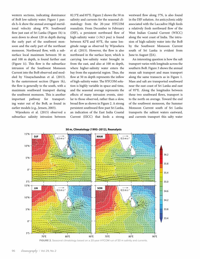
westward flow along 5°N, is also found in the DJF solution. An anti cyclonic eddy associated with the Laccadive High feeds a relatively fresh northward flow of the West Indian Coastal Current (WICC) along the west coast of India. The intru-sion of high- salinity water into the BoB by the Southwest Monsoon Current south of Sri  Lanka is evident from June to August (JJA).

An interesting question is how the salt transport varies with longitude across the southern BoB. Figure 3 shows the annual mean salt transport and mass transport along the same transects as in Figure  1. Mass and salt are transported southward near the east coast of Sri Lanka and east of 95°E. Along the longitudes between these two southward flows, transport is to the north on average. Toward the end of the southwest monsoon, the Summer Monsoon Current south of Sri  Lanka transports the saltiest waters eastward, and currents transport this salty water

FIGURE 2. Seasonal climatology based on a 20-year HYCOM run of 50 m salinity and currents.

82.5°E and 85°E. Figure 2 shows the 50 m salinity and currents for the seasonal cli-matology from the 20-year HYCOM reanalysis. From December to February (DJF), a persistent northward flow of high- salinity water (>34.5 psu) is found between 82°E and 85°E, the same lon-gitude range as observed by Wijesekera et  al. (2015). However, the flow is also northward in the surface layer, which is carrying low- salinity water brought in from the east, and also at 100 m depth, where higher- salinity water enters the bay from the equatorial region. Thus, the flow at 50 m depth represents the inflow of high- salinity water. The HYCOM solu-tion is highly variable in space and time, and the seasonal average represents the effects of many intrusion events, simi-lar to those observed, rather than a slow, broad flow as shown in Figure 2. A strong persistent southward flow past Sri Lanka, an indication of the East India Coastal Current (EICC) that feeds a strong

western sections, indicating dominance of BoB low-salinity water. Figure 1 pan-els h–k show the annual averaged merid-ional velocity along 8°N. Southward flow just east of Sri Lanka (Figure 1h) is seen down to about 120 m depth during the early part of the southwest mon-soon and the early part of the northeast monsoon. Northward flow, with a sub-surface local maximum between 50 m and 100 m depth, is found further east (Figure 1i). This flow is the subsurface intrusion of the Southwest Monsoon Current into the BoB observed and mod-eled by Vinayachandran et  al. (2013). In the easternmost section (Figure 1k), the flow is generally to the south, with a maximum southward transport during the southwest monsoon. This is another important pathway for transport-ing water out of the BoB, as found in earlier models (e.g., Jensen, 2003).

Wijesekera et  al. (2015) observed a subsurface salinity intrusion between

50 m, Climatology (1993–2012), Reanalysis

DJF MAM

JJA SON

70°E

15°N

36.2

35.8

35.4

35.0

34.6

34.2

33.8

33.4

10°N

5°N

0°

5°S

15°N

10°N

5°N

0°

5°S

80°E 90°E 70°E 80°E 90°E

0.5 m s–1

0.5 m s–10.5 m s–1

0.5 m s–1

Oceanography | June 2016 97

FIGURE 3. Mean salt transport (× 107 kg s–1) integrated through the entire water column. All data points at each latitude and longitude are plotted. (right) Corresponding mean mass transport (× 109 kg s–1). Background color is sea surface salinity.

Salt Transport

(a) Annual Mean

(b) Sep Mean

(c) Dec Mean

(d) Annual Mean

(e) Sep Mean

(f) Dec Mean

Mass Transport

25°N

25°N

25°N

5°N

5°N

5°N

15°N

15°N

15°N

5°S

5°S

5°S

70°E 90°E 90°E80°E 80°E100°E 100°E

32 34 36 38

northward, to the east of Sri  Lanka. On the other hand, the maximum trans-ports during the northeast monsoon sea-son appear early in December. There is a strong southward salt flux past Sri Lanka that is connected to a westward salt trans-port, a result expected from drifter obser-vations (Wijesekera et al., 2015). An inter-esting feature is the alternating directions of the zonal mass and salt transports between Sri Lanka and the equator.

Importance of Rivers Demonstrated by the Regional Indian Ocean Model The ROMS simulated fields were vali-dated against observations. Ocean Surface Current Analyses Real time (OSCAR) monthly mean sea surface currents pro-vided by the US National Oceanic and Atmospheric Administration (http://www.oscar.noaa.gov) were used to assess the currents simulated by the model. Bonjean and Lagerloef (2002) describe the methodology adopted in OSCAR to calculate the ocean near-surface hori-zontal currents from satellite measure-ments of sea surface height, wind stress, and sea surface temperature. Salinity simulations from ROMS were com-pared with the North Indian Ocean Atlas by Chatterjee et al. (2012); these are the most recently launched climatologi-cal data sets of temperature and salin-ity exclusive for the North Indian Ocean. The sea surface salinity (SSS) simulated by the ROMS model agrees well with observations over most of the domain (Figure  4). However, the northern Bay of Bengal low-salinity plumes, particu-larly during July–November, were not captured well by the model. SSS variabil-ity in the northern BoB is influenced by significant freshwater contributions from

20°N

20°N

0°

0°

20°S

20°S

60°E 60°E90°E 90°E

.6 m s–1

28 32 3630 34 3829 33 3731 35

ROMS

Jan

Jul

Jan

Jul

NIOA

FIGURE  4. Comparison of model simu-lated sea surface salinity (psu) and currents (m s–1) in the Regional Ocean Modeling System (ROMS) with climatological North Indian Ocean Atlas (NIOA) surface salinity and Ocean Surface Current Analyses Real time (OSCAR; http://www.oscar.noaa.gov) currents for the months of January and July.

Oceanography | Vol.29, No.298

to the equatorial region. When eastward- flowing equatorial jets associated with intraseasonal oscillations are present, for instance the westerly wind bursts during the active phase of the MJO (e.g., Jensen et al., 2015), these intrusions into the BoB can take place (Wijesekera et al., 2015).

The currents and salinity at 50 m depth from December 2013 (Figure 5, top panel) reveal the complex flow pattern of a salinity intrusion. An anticyclonic eddy pair situated at 84°E–87°E, 13°N–15°N prevents further northward advection of the salinity intrusion. The simulation also shows a remarkably narrow but continu-ous southward flow of the EICC, starting from 17°N until it turns westward south of Sri Lanka. A south-to-north cross sec-tion along 84°E (white dashed line in Figure  5, top panel) through the high- salinity intrusion (Figure 5, bottom panel) indicates a very strong vertical gradient at 50 m depth between the low-salinity water in the mixed layer and the high- salinity intrusion that appears as a local salinity maximum. The local maximum is found as far north as 10°N, overlying the deeper 35 psu water found below 100 m in the southern BoB and below 150 m further north. The cross section reveals salinity inversions, which suggest vertical mixing. Intermediate salinity of 34.5 psu found north of 10°N between 50 m and 150 m depth also implies that mixing has occurred. These results are consis-tent with the Argo observations shown by Gordon et al. (2016, in this issue; see their Figure 7a).

From the COAMPS run, the verti-cal diffusion coefficients produced by the Mellor-Yamada scheme are available. Figure 6 shows a typical cross section of diffusion in the BoB. Vertical mixing is very large in the mixed layer above the thermocline near 60 m. In the thermo-cline and at deeper levels, only sporadic bursts of vertical diffusion are found. The propagation of solitary-like semi-diurnal internal waves, resulting from tides in the Andaman Sea, can reach deep into the thermocline and increase diffu-sion locally in time and space by several

FIGURE  5. (top) Daily averaged salinity and currents at 50 m depth on December 24, 2013, from the Coupled Ocean–Atmosphere Mesoscale Prediction System (COAMPS). (bottom) Salinity and meridional current component along 84.0°E (white dashed line in top panel) on December 18, 2013, from COAMPS. Contour interval is 0.2 m s–1. Full black line is northward flow, and black dashed line is southward flow. Zero contour is not shown.

uv (50.0 m) salint (50.0 m) and seatmp (50.0 m) 2013122400 24 hours

Salinity and meridional velocity 84°E 2013 121800 12 hours

20°N

10°N

15°N

5°N

0°0°

0

50

100

150

200

250

Dep

th (m

)

70°E

5°N 7°N 10°N 13°N

36.0

33.0

34.5

35.5

32.5

34.0

35.0

32.0

33.5

35

34

336°N 9°N

Latitude12°N8°N 11°N

80°E 95°E75°E 90°E85°E

0.5 m s–1

more realistic simulation of the environ-ment than stand-alone ocean models. For instance, during the northeast monsoon, HYCOM solutions indicated a northward flow of relatively high-salinity water. In the high-resolution COAMPS model, we found that these intrusions occur during events that are highly variable in space and time. The figure on this arti-cle’s title page shows such an event, where subsurface flow of high-salinity water (>35 psu) intrudes into the southern BoB. This water subsequently spreads out along isopycnals as it subducts deeper into the bay, advecting high-salinity water to the north in an eddying motion. As the fig-ure shows, this water can be traced back

the Ganges and Brahmaputra Rivers (Pant et al., 2015). Thus, it is essential to include the river discharges in the model to correctly simulate SSS in the northern BoB. The model is able to simulate sea-sonally reversing currents (i.e.,  Summer and Winter Monsoon Currents, EICC, WICC, and Somali Current).

Subduction and Intrusion into the Bay of Bengal Simulated by COAMPSThe high spatial resolution of the ocean current and wind field, the tight cou-pling between the ocean and the atmo-sphere, and the presence of surface waves and tides in COAMPS can give a

36

Oceanography | June 2016 99

orders of magnitude, according to recent work of author Jensen and colleagues. However, in general, the vertical diffusion is found to be very small in the interior of the BoB, at least in the model solution. That raises the question: How do low- salinity and high-salinity waters mix in the model and in the real ocean?

As mentioned above, the intruding high-salinity water propagates north-ward along surfaces of constant den-sity (i.e.,  isopycnals). Also, along the same density surface, colder low-salinity water spreads southward. Figure 7 shows the salinity on the 1,024 kg m–3 density surface. Note that there are salinity dif-ferences of 0.5 psu at distances of a few kilometers. Stirring by eddies stretches these salinity filaments. In the numer-ical ocean models, diffusion associated with the numerical scheme (in the case of COAMPS, a third-order upstream scheme with flux correction) will remove these gradients when their scales become comparable with the grid resolution. As Gordon et al. (2016, in this issue) discuss, observations appear to support the sub-duction, advection, and stirring scenario along constant density surfaces, followed by mixing at small-scales.

SUMMARY AND CONCLUSIONSThree different ocean models with vary-ing complexity are used to simulate salin-ity in the region where ASIRI observa-tions were collected. The models show that salinity exchanges between the equa-torial Indian Ocean and the Bay of Bengal dominate during the southwest monsoon. This is in agreement with earlier modeling studies (Vinayachandran et al., 1999; Han and McCreary, 2001; Jensen, 2001, 2003). Global HYCOM shows higher-salinity inflow during the northeast monsoon as well. On average, salt is transported into the BoB between 83°E and 95°E and out of the BoB by southward flow near the east coast of Sri Lanka and east of 95°E. The lower-salinity of waters in the two lat-ter regions indicates they are the pathways taken by freshwater from rivers, runoff, and precipitation out of the BoB. This is

0

20

40

60

80

100

120D

epth

(m)

Vertical eddy diffusion and temperature 5.0°N 2014 030812 06 hours

85°E 89°E87°E 91°E86°E 90°E88°ELongitude

FIGURE 6. Vertical eddy diffusion coefficient (log 10 based) shown in color. Isolines show temperature (contour interval 1°C). The white contour is the 20°C isotherm. Isotherms of 18°C and above are shown as solid lines.

FIGURE 7. Daily averaged salinity and currents at the 24.0 σt surface on August 15, 2015, from COAMPS.

20°N

10°N

15°N

0°

5°N

Current surface sigsal on 24.0 σt and sigsal 2015 081500 00 hours

70°E 90°E80°E75°E 95°E85°E

psu36.0

35.5

35.0

34.5

34.0

33.5

33.0

0.5 m s–1

RAMA

–5.0 –3.0–4.0 –2.0–4.5 –2.5–3.5

Oceanography | Vol.29, No.2100

in agreement with the results from simple layer models (e.g., Jensen, 2003) and sup-ported by observations (Sengupta et  al., 2006; Gordon et al., 2016, in this issue).

The regional Indian Ocean model based on ROMS reveals that it is essential to include river input for accurate mod-eling of surface salinities in the Indian Ocean; however, models are able to reproduce the general circulation in the tropical Indian Ocean, as it is dominated by wind forcing. This result also corrob-orates those produced using a simpler layer model (Han and McCreary, 2001).

By using a high horizontal and high vertical resolution ocean model tightly coupled to a regional atmosphere model, we find that intrusion of high- salinity water is through subsurface flow during both the southwest and north-east monsoon seasons. Observations by Wijesekera et  al. (2015) showed veloci-ties over 1 m s–1 for this flow during the northeast monsoon in December 2013. In the high-resolution model, this sub-surface flow spreads northward along isopycnals. In the model, stirring brings cold, low-salinity water from the north-ern Bay of Bengal in close contact with warm, high-salinity water from the equa-torial region, and permits mixing, in par-ticular north of 10°N.

The model simulations are helpful for understanding the field experiments in the context of regional ocean circulation.

Output from all three models is being made available to ASIRI researchers to permit comparison with observations and to help interpret their findings.

suppressed phase. Journal of Atmospheric Science 72:3,755–3,779, http://dx.doi.org/10.1175/JAS-D-13-0348.1.

Fairall, C.W., E.F. Bradley, J.S. Godfrey, G.A. Wick, J.B. Edson, and G.S. Young. 1996a. Cool-skin and warm-layer effects on sea sur-face temperature. Journal of Geophysical Research 101(C1):1,295–1,308, http://dx.doi.org/ 10.1029/95JC03190.

Fairall, C.W., E.F. Bradley, D.P. Rogers, J.B. Edson, and G.S. Young. 1996b. Bulk parameteriza-tion of air-sea fluxes for Tropical Ocean-Global Atmosphere Coupled-Ocean Atmosphere Response Experiment. Journal of Geophysical Research 101(C2):3,747–3,764, http://dx.doi.org/ 10.1029/95JC03205.

Gordon, A.L., E.L. Shroyer, A. Mahadevan, D. Sengupta, and M. Freilich. 2016. Bay of Bengal: 2013 northeast monsoon upper-ocean circulation. Oceanography 29(2):82–91, http://dx.doi.org/10.5670/oceanog.2016.41.

Haidvogel, D.B., H. Arango, W.P. Budgell, B.D. Cornuelle, E. Curchitser, E. Di Lorenzo, K. Fennel, W.R. Geyer, A.J. Hermann, L. Lanerolle, and others. 2008. Ocean forecasting in ter-rain-following coordinates: Formulation and skill assessment of the Regional Ocean Modeling System. Journal of Computational Physics 227(7):3,595–3,624, http://dx.doi.org/ 10.1016/j.jcp.2007.06.016.

Haidvogel, D.B., H.G. Arango, K. Hedstrom, A. Beckmann, P. Malanotte-Rizzoli, and A.F. Shchepetkin. 2000. Model evaluation exper-iments in the North Atlantic Basin: Simulations in nonlinear terrain-following coordinates. Dynamics of Atmospheres and Oceans 32(3):239–281, http://dx.doi.org/10.1016/S0377-0265(00)00049-X.

Han, W. 2005. Origins and dynamics of the 90-day and 30–60 day variations in the equa-torial Indian Ocean. Journal of Physical Oceanography 35:708–728, http://dx.doi.org/ 10.1175/JPO2725.1.

Han, W., and J.P. McCreary Jr. 2001. Modeling salinity distributions in the Indian Ocean. Journal of Geophysical Research 106:859–877, http://dx.doi.org/10.1029/2000JC000316.

Jensen, T.G. 1993. Equatorial variabil-ity and resonance in a wind-driven Indian Ocean model. Journal of Geophysical Research 98:22,533–22,552, http://dx.doi.org/ 10.1029/93JC02565.

Jensen, T.G. 2001. Arabian Sea and Bay of Bengal exchange of salt and tracers in an ocean model. Geophysical Research Letters 28:3,967–3,970, http://dx.doi.org/10.1029/2001GL013422.

Jensen, T.G. 2003. Cross-equatorial pathways of salt and tracers from the northern Indian Ocean: Modelling results. Deep Sea Research Part II 50:2,111–2,128, http://dx.doi.org/10.1016/S0967-0645(03)00048-1.

Jensen, T.G., T. Shinoda, S. Chen, and M. Flatau. 2015. Ocean response to CINDY/DYNAMO MJOs in air-sea coupled COAMPS. Journal of the Meteorological Society of Japan 93A:157–178, http://dx.doi.org/10.2151/jmsj.2015-049.

Kantha, L.H., and C.A. Clayson. 2004. On the effect of surface gravity waves on mixing in the oce-anic mixed layer. Ocean Modelling 6:101–124, http://dx.doi.org/10.1016/S1463-5003(02)00062-8.

Large, W.G., J.C. McWilliams, and S.C. Doney. 1994. Oceanic vertical mixing: A review and a model with a nonlocal boundary layer parameteriza-tion. Reviews of Geophysics 32(4):363–403, http://dx.doi.org/10.1029/94RG01872.

Locarnini, R.A., A.V. Mishonov, J.I. Antonov, T.P. Boyer, H.E. Garcia, O.K. Baranova, M.M. Zweng, and D.R. Johnson. 2010. World Ocean Atlas 2009:

“Three different ocean models with varying complexity are used to simulate salinity in the region where ASIRI observations were collected. The models show that salinity exchanges between the equatorial Indian Ocean and the Bay of Bengal dominate during the southwest monsoon.

”.

REFERENCESAntonov, J., D. Seidov, T. Boyer, R. Locarnini,

A. Mishonov, H. Garcia, O. Baranova, M. Zweng, and D. Johnson. 2010. World Ocean Atlas 2009: Volume 2, Salinity. S. Levitus, ed., US Government Printing Office, Washington, DC, 184 pp, ftp://ftp.nodc.noaa.gov/pub/WOA09/DOC/woa09_vol2_text.pdf.

Bleck, R. 2002. An oceanic general circulation model framed in hybrid isopycnic-Cartesian coordinates. Ocean Modelling 4:55–88, http://dx.doi.org/10.1016/S1463-5003(01)00012-9.

Bleck, R., and S.G. Benjamin. 1993. Regional weather prediction with a model combining terrain-following and isentropic coordinates: Part 1. Model descrip-tion. Monthly Weather Review 121(6):1,770–1,785, http://dx.doi.org/10.1175/1520-0493(1993)121 <1770:RWPWAM>2.0.CO;2.

Bleck, R., and D.B. Boudra. 1981. Initial testing of a numerical ocean circulation model using a hybrid (quasi–isopycnic) vertical coordinate. Journal of Physical Oceanography 11(6):755–770, http://dx.doi.org/10.1175/1520-0485(1981)011 <0755:ITOANO>2.0.CO;2.

Bonjean, F., and G.S. Lagerloef. 2002. Diagnostic model and analysis of the surface currents in the tropical Pacific Ocean. Journal of Physical Oceanography 32(10):2,938–2,954, http://dx.doi.org/10.1175/1520-0485(2002)032 <2938:DMAAOT>2.0.CO;2.

Booij, N., R.C. Ris, and L.H. Holthuijsen. 1999. A third-generation wave model for coastal regions: Part I. Model description and validation. Journal of Geophysical Research 104:7,649–7,666, http://dx.doi.org/10.1029/98JC02622.

Chatterjee, A., D. Shankar, S.S.C. Shenoi, G.V. Reddy, G.S. Michael, M. Ravichandran, V.V. Gopalkrishna, E.R. Rao, T.U. Bhaskar, and V.N. Sanjeevan. 2012. A new atlas of temperature and salinity for the North Indian Ocean. Journal of Earth System Science 121(3):559–593, http://dx.doi.org/10.1007/s12040-012-0191-9.

Chen, S., M. Flatau, T.G. Jensen, T. Shinoda, J. Schmidt, P. May, J. Cummings, M. Liu, P.E. Ciesielski, C.W. Fairall, and others. 2015. A study of CINDY/DYNAMO MJO

Oceanography | June 2016 101

Volume 1, Temperature. S. Levitus, ed., NOAA Atlas NESDIS, 68, 184 pp, ftp://ftp.nodc.noaa.gov/pub/WOA09/DOC/woa09_vol1_text.pdf.

Love, B.S., A.J. Matthews, and G.S. Lister, 2011. The diurnal cycle of precipitation over the Maritime Continent in a high-resolution atmo-spheric model. Quarterly Journal of the Royal Meteorology Society 137:934–947, http://dx.doi.org/10.1002/qj.809.

Matsuno, T. 1966. Quasi-geostrophic motions in the equatorial area. Journal of the Meteorological Society of Japan 44:25–43.

McCreary, J.P., W. Han, D. Shankar, and S.R. Shetye, 1996. Dynamics of the East India Coastal Current: Part 2. Numerical solutions. Journal of Geophysical Research 101:13,993–14,010, http://dx.doi.org/ 10.1029/96JC00560.

Mellor, G.L., and T. Yamada. 1982. Development of a turbulence closure model for geophysical fluid problems. Reviews of Geophysics and Space Physics 20:851–875, http://dx.doi.org/10.1029/RG020i004p00851.

Metzger, E.J., H.E. Hurlburt, X. Xu, J.F. Shriver, A.L. Gordon, J. Sprintall, R.D. Susanto, and H.M. van Aken. 2010. Simulated and observed circulation in the Indonesian Seas: 1/12° global HYCOM and the INSTANT observations. Dynamics of Atmospheres and Oceans 50:275–300, http://dx.doi.org/10.1016/j.dynatmoce.2010.04.002.

Metzger, E.J., O.M. Smedstad, P.G. Thoppil, H.E. Hurlburt, J.A. Cummings, A.J. Wallcraft, L. Zamudio, D.S. Franklin, P.G. Posey, M.W. Phelps, and others. 2014. US Navy operational global ocean and Arctic ice prediction systems. Oceanography 27(3):32–43, http://dx.doi.org/ 10.5670/oceanog.2014.66.

Murty, V.S.N., Y.V.B. Sarma, D.P. Rao, and C.S. Murty. 1992. Water characteristics, mixing and circula-tion in the Bay of Bengal during southwest mon-soon. Journal of Marine Research 50:207–228, http://dx.doi.org/10.1357/002224092784797700.

Pant, V., M.S. Girishkumar, T.V.S. Udaya Bhaskar, M. Ravichandran, F. Papa, and V.P. Thangaprakash. 2015. Observed interannual variability of near-sur-face salinity in the Bay of Bengal. Journal of Geophysical Research 120:3,315–3,329, http://dx.doi.org/10.1002/2014JC010340.

Praveen Kumar, B., J. Vialard, M. Lengaigne, V.S. Murty, and M.J. McPhaden. 2012. TropFlux: Air-sea fluxes for the global tropi-cal oceans: Description and evaluation. Climate Dynamics 38:1,521–1,543, http://dx.doi.org/10.1007/s00382-011-1115-0.

Qiu, B., M. Mao, and Y. Kashino. 1999. Intraseasonal variability in the Indo-Pacific throughflow and regions surrounding the Indonesian seas. Journal of Physical Oceanography 29:1,599–1,618, http://dx.doi.org/10.1175/1520-0485(1999)029 <1599:IVITIP>2.0.CO;2.

Saha, S., S. Moorthi, H.-L. Pan, X. Wu, J. Wang, S. Nadiga, P. Tripp, R. Kistler, J. Woollen, D. Behringer, and others. 2010. The NCEP cli-mate forecast system reanalysis. Bulletin of the American Meteorological Society 91:1,015–1,057, http://dx.doi.org/10.1175/2010BAMS3001.1.

Shchepetkin, A.F., and J.C. McWilliams. 2003. A method for computing horizontal pres-sure-gradient force in an oceanic model with a nonaligned vertical coordinate. Journal of Geophysical Research 108(C3), 3090, http://dx.doi.org/10.1029/2001JC001047.

Shchepetkin, A.F., and J.C. McWilliams. 2005. The Regional Oceanic Modeling System (ROMS): A split-explicit, free-surface, topography- following-coordinate oceanic model. Ocean Modelling 9(4):347–404, http://dx.doi.org/10.1016/ j.ocemod.2004.08.002.

Shchepetkin, A.F., and J.C. McWilliams. 2009. Computational kernel algorithms for fine-scale, multiprocess, longtime oceanic simulations. Handbook of Numerical Analysis 14:121–183, http://dx.doi.org/10.1016/S1570-8659(08)01202-0.

Sengupta, D., G.N. Bharath Raj, and S.S.C. Shenoi. 2006. Surface freshwater from Bay of Bengal run-off and Indonesian Throughflow to the tropical Indian Ocean. Geophysical Research Letters 33, L22609, http://dx.doi.org/10.1029/2006GL027573.

Shinoda, T., W. Han, E.J. Metzger, and H. Hurlburt. 2012. Seasonal variation of the Indonesian Throughflow in Makassar Strait. Journal of Physical Oceanography 42:1,099–1,123, http://dx.doi.org/ 10.1175/JPO-D-11-0120.1.

Smith, W.H.F., and D.T. Sandwell. 1997. Global sea floor topography from satellite altimetry and ship depth soundings. Science 277:1,956–1,962, http://dx.doi.org/10.1126/science.277.5334.1956.

Thoppil, P.G., E.J. Metzger, H.E. Hurlburt, O.M. Smedstad, and H. Ichikawa. 2016. The current system east of the Ryukyu Islands as revealed by a global ocean reanaly-sis. Progress in Oceanography 141:239–258, http://dx.doi.org/10.1016/j.pocean.2015.12.013.

Vinayachandran, P.N., Y. Masumoto, T. Mikawa, and T. Yamagata. 1999. Intrusion of the Southwest Monsoon Current into the Bay of Bengal. Journal of Geophysical Research 104:11,077–11,085, http://dx.doi.org/10.1029/1999JC900035.

Vinayachandran, P.N., D. Shankar, S. Vernekar, K.K. Sandeep, P. Amol, C.P. Neema, and Abhisek Chatterjee. 2013. A summer monsoon pump to keep the Bay of Bengal salty. Geophysical Research Letters 40:1,777–1,782, http://dx.doi.org/ 10.1002/grl.50274.

Wijesekera, H.W., T.G. Jensen, E. Jarosz, W.J. Teague, E.J. Metzger, D.W. Wang, S.U.P. Jinadasa, K. Arulananthan, L.R. Centurioni, and H.J. Fernando. 2015. Southern Bay of Bengal currents and salin-ity intrusions during the northeast monsoon. Journal of Geophysical Research 120:6,897–6,913, http://dx.doi.org/10.1002/2015JC010744.

Yu, L., J.J. O’Brien, and J. Yang. 1991. On the remote forcing of the circulation in the Bay of Bengal. Journal of Geophysical Research 96:20,449–20,454, http://dx.doi.org/ 10.1029/91JC02424.

ACKNOWLEDGMENTSThe authors would like to thank Jan Dastugue, Naval Research Laboratory (NRL), for assistance with graphics. This research has been sponsored by the US Office of Naval Research (ONR) in an ONR Departmental Research Initiative: Air-Sea Interactions Regional Initiative (ASIRI), and in a US Naval Research Laboratory basic research project: Effects of Bay of Bengal Freshwater Flux on Indian Monsoon (EBOB). Additional funding was granted from the Ocean Mixing and Monsoon (OMM) project under the National Monsoon Mission (NMM) of the Government of India. This is NRL contribution number JA/7320-16-3015.

COAMPS® is a registered trademark of the Naval Research Laboratory.

AUTHORSTommy G. Jensen is Oceanographer, Hemantha W. Wijesekera is Oceanographer, Prasad G. Thoppil is Oceanographer, and Jay F. Shriver is Oceanographer, all at the US Naval Research Laboratory, Stennis Space Center, MS, USA. Ebenezer S. Nyadjro is a researcher in the Department of Physics, University of New Orleans, New Orleans, LA, USA. K.K. Sandeep is a graduate

student and Vimlesh Pant is Assistant Professor at the Centre for Atmospheric Sciences, Indian Institute of Technology Delhi, New Delhi, India.

ARTICLE CITATIONJensen, T.G., H.W. Wijesekera, E.S. Nyadjro, P.G. Thoppil, J.F. Shriver, K.K. Sandeep, and V. Pant. 2016. Modeling salinity exchanges between the equatorial Indian Ocean and the Bay of Bengal. Oceanography 29(2):92–101, http://dx.doi.org/10.5670/oceanog.2016.42.