CITATION

Zhao, Z., M.H. Alford, and J.B. Girton. 2012. Mapping low-mode internal tides from multisatellite

altimetry. Oceanography 25(2):42–51, http://dx.doi.org/10.5670/oceanog.2012.40.

DOI

http://dx.doi.org/10.5670/oceanog.2012.40

COPYRIGHT

This article has been published in Oceanography, Volume 25, Number 2, a quarterly journal of

The Oceanography Society. Copyright 2012 by The Oceanography Society. All rights reserved.

USAGE

Permission is granted to copy this article for use in teaching and research. Republication,

systematic reproduction, or collective redistribution of any portion of this article by photocopy

machine, reposting, or other means is permitted only with the approval of The Oceanography

Society. Send all correspondence to: info@tos.org or The Oceanography Society, PO Box 1931,

Rockville, MD 20849-1931, USA.

OceanographyTHE OffICIAl MAGAZINE Of THE OCEANOGRAPHY SOCIETY

DOwNlOADED fROM HTTP://www.TOS.ORG/OCEANOGRAPHY

Oceanography | Vol. 25, No. 242

54°N

50°N

45°N

40°N

35°N

30°N

25°N

20°N

180°W 175°W 170°W 165°W 160°W 155°W

54°N

50°N

45°N

40°N

35°N

30°N

25°N

20°N

180°W 175°W 170°W 165°W 160°W 155°W

30

24

18

12

6

0

Am

plitu

de (m

m)

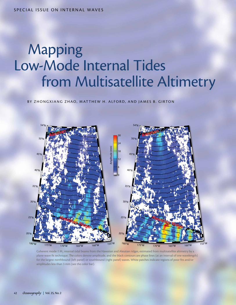
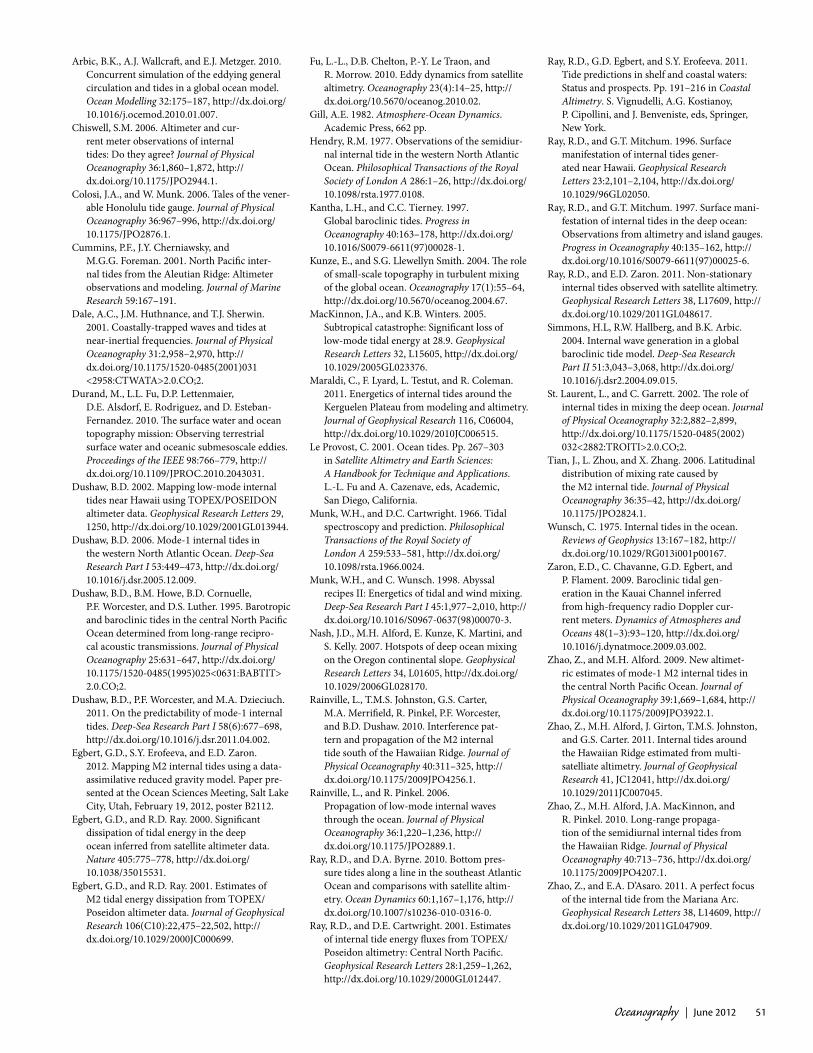
Coherent mode-1 M2 internal tidal beams from the Hawaiian and Aleutian ridges, estimated from multisatellite altimetry by a plane-wave fit technique. The colors denote amplitude, and the black contours are phase lines (at an interval of one wavelength) for the largest northbound (left panel) or southbound (right panel) waves. White patches indicate regions of poor fits and/or amplitudes less than 3 mm (see the color bar).

MappingLow-Mode Internal Tides

from Multisatellite AltimetryB y Z H o N g x I A N g Z H A o , M AT T H e W H . A L f o r d , A N d J A M e s B . g I r T o N

s p e C I A L I s s u e o N I N T e r N A L WAV e s

Oceanography | Vol. 25, No. 242

Oceanography | June 2012 43

INTerNAL TIdesAbout 1 TW (1012 W) of power is lost from the surface tide in the deep ocean at rough bottom topography such as seamounts, ridges, and trenches (Egbert and Ray, 2000, 2001). A major fraction (~ 80%) of the power is converted into low-mode internal tides (i.e., internal waves of tidal frequency and long vertical wavelengths; see Figure 1) and trans-ported thousands of kilometers from the generation sites (Dushaw et al., 1995; Ray and Cartwright, 2001; Alford, 2003; Zhao and Alford, 2009). Internal tides may dissipate upon encountering strongly sheared currents, scattering on the rough seafloor, and cascading to small-scale waves through processes such as para-metric subharmonic instability (PSI; e.g., St. Laurent and Garrett, 2002; Kunze and Llywellyn Smith, 2004; MacKinnon and Winters, 2005; Alford et al., 2007). The portion that does not dissipate via one of these mechanisms is thought to do so when it encounters distant continental slopes (e.g., Nash et al., 2007). The role of these mechanisms in the eventual dis-sipation of internal tides remains an open question. The geographic distribution of tidal energy dissipation is important for

large-scale ocean circulation, climate, and biological productivity (Munk and Wunsch, 1998; St. Laurent and Garrett, 2002). Thus, mapping internal tides from their generation sites to their dissipation sites may advance our knowledge of their dynamics. Internal tides are tradition-ally measured by in situ observations of their velocity and displacement profiles (Wunsch 1975; Alford 2003). However, the sparse distribution of these mea-surements limits in-depth knowledge of the internal tide field, particularly on a global scale.

INTerNAL TIdes IN A roTATINg sTr ATIfIed oCeANOcean stratification is described by the buoyancy frequency profile

N(z) = (– )1/2gρ0

dρ(z)dz ,

where g is gravitational acceleration, ρ0 is a reference ocean water density, ρ(z) is potential density, and z is verti-cal coordinate (positive upward). An internal tide in a continuously stratified ocean can be represented by a sum of discrete baroclinic modes that depend only on the buoyancy frequency profile N(z) and the water depth H. The modes

are then described by the eigenvalue equation (Gill, 1982):

+ Φ(z) = 0,N 2(z)cn

2

d2Φ(z)dz2

(1)

subject to rigid-lid boundary condi-tions Φ(0) = Φ(H) = 0, where Φ(z) is the eigenfunction and cn the eigenvalue for the nth mode. The term Φ(z) describes the baroclinic modal structures for dis-placement and vertical velocity; Π(z) describes the equivalent structures for horizontal velocity and pressure and is related to Φ(z) via

Π(z) = ρ0cn2 .dΦ(z)

dzThe effect of Earth’s rotation is described by the local inertial fre-quency f = 2Ωsin(latitude), where Ω (= 7.3 × 10–5 rad s–1) is Earth’s rota-tion rate. The phase velocity cp can be obtained as

cp = cn, ωω2 – f 2

where ω is the tidal frequency (Rainville and Pinkel, 2006).

Typically, we solve Equation 1 for the four lowest baroclinic modes in a strati-fied deep ocean (Figure 1a). The normal-ized Φ(z) and Π(z) (Figure 1b,c, respec-tively) have wavelengths 154, 77, 52, and 40 km for modes 1–4, respectively. While the barotropic tide may have wave-lengths of thousands of kilometers, inter-nal tidal wavelengths are much shorter.

Though the rigid-lid approximation is used to solve the eigenvalue equation, Φ(z) is not zero at the sea surface. Via their pressure fluctuations Π(z) at the sea surface (Figure 1c), internal tides deflect the sea surface by several centimeters. Taking Figure 1 as an example, for a 10 m maximum internal amplitude, the sea surface amplitudes are 1.8, 0.6, 0.4, and 0.2 cm for modes 1–4, respectively. Lower

ABsTr AC T. Low-mode internal tides propagate over thousands of kilometers from their generation sites, distributing tidal energy across the ocean basins. Though internal tides can have large vertical displacements (often tens of meters or more) in the ocean interior, they deflect the sea surface only by several centimeters. Because of the regularity of the tidal forcing, this small signal can be detected by state-of-the-art, repeat-track, high-precision satellite altimetry over nearly the entire world ocean. Making use of combined sea surface height measurements from multiple satellites (which together have denser ground tracks than any single mission), it is now possible to resolve the complex interference patterns created by multiple internal tides using an improved plane-wave fit technique. As examples, we present regional M2 internal tide fields around the Mariana Arc and the Hawaiian Ridge and in the North Pacific Ocean. The limitations and some perspective on the multisatellite altimetric methods are discussed.

Oceanography | Vol. 25, No. 244

modes have greater sea surface amplitude for the same interior amplitude.

Conversely, the interior amplitude can be estimated from the sea surface amplitude. Thus, energy and flux can be calculated and are proportional to amplitude squared. From the hydro-graphic profiles, the vertical structures and propagation speeds of low-mode internal tides can be determined in the world ocean (Rainville and Pinkel, 2006). In addition, the functional relations from sea surface amplitude to energy and flux can be determined (Chiswell, 2006; Zhao and Alford, 2009).

The internal tidal frequency must be greater than the local near-inertial frequency, that is, ω ≥ f. For the diur-nal and semidiurnal internal tides, this requirement gives rise to “turning lati-tudes” of about 29° and 75°, respectively. Progressive internal tides do not exist

in the open ocean poleward of turn-ing latitudes (Dushaw, 2006; Rainville and Pinkel, 2006), although topo-graphically trapped solutions may exist (e.g., Dale et al., 2001).

INTerNAL TIdes froM sATeLLITe ALTIMeTrySea surface height (SSH) variations induced by internal tides have long been observed as tidal “cusps” around discrete tidal lines in frequency spectra (Munk and Cartwright, 1966; Colosi and Munk, 2006). However, explor-ing these weak signals over basin scales only became practical with the advent of satellite altimetry (Ray and Mitchum, 1996, 1997). Satellite altimetry can measure SSH with an accuracy of about 2 cm. Its measurement errors σ are distributed over a wide range of the spectrum. Therefore, to extract tidal

signals (with their precisely known frequencies), the errors scale as σ/ N , where N is the number of measurements. Thus, with a sufficient number (several hundreds) of measurements, satellite altimetry may resolve tidal signals with 1–2 mm resolution.

The orbit parameters of satellite altimeters are such that they repeat their ground tracks at intervals of tens of days (Table 1), periods much longer than the semidiurnal and diurnal tidal periods (0.5 and 1 day). This aliases tidal signals to long periods that are different for each altimeter. For example, for the TOPEX/Poseidon (T/P) altimeter, M2 and S2 tides alias to 62.11 and 58.74 days, respec-tively. It is remarkable that internal tides can be studied with a dataset exhibiting sampling only once every 20–60 wave periods. Harmonic analysis over many samples is used to extract the signal at each tidal frequency. The method relies on the coherence of internal tides such that phase is largely maintained from sample to sample. It is only this tempo-rally coherent portion of the signal that is detectable by altimetry, a point we return to later.

0 2 4 6

0

1000

2000

3000

4000

4870

N (cycles per hour)

Dep

th (m

)

(a)

−1.0 −0.5 0.0 0.5 1.0Displacement; Vertical velocity

(b)

−1.0 −0.5 0.0 0.5 1.0Pressure; Horizontal velocity

(c)

M2 Wavelength mode 1: 153.8 km mode 2: 76.3 km mode 3: 52.2 km mode 4: 38.7 km

figure 1. (a) Buoyancy fre-quency profile at 25.5°N, 195°e from the World ocean Atlas database. The four lowest baroclinic modes are solutions of equation 1. (b) Normalized baroclinic modal structures for displacement and vertical veloc-ity. (c) Normalized baroclinic modal structures for horizontal velocity and pressure. The wave-lengths of modes 1–4 M2 inter-nal tides are given.

Zhongxiang Zhao (zzhao@apl.washington.edu) is Senior Oceanographer, Applied

Physics Laboratory, University of Washington, Seattle, WA, USA. Matthew H. Alford is

Principal Oceanographer, Applied Physics Laboratory, and Associate Professor, School of

Oceanography, University of Washington, Seattle, WA, USA. James B. Girton is Senior

Oceanographer, Applied Physics Laboratory, and Affiliate Assistant Professor, School of

Oceanography, University of Washington, Seattle, WA, USA.

Oceanography | June 2012 45

Table 1. satellite altimeter data: Topex/poseidon (T/p), Jason-1 (J1), Jason-2 (J2), geosat follow-on (gfo), european remote sensing (ers)

DatasetSatellite

AltimeterRepeat

Period (day)Total

TracksTrack Spacing

(km)*Data Period (mm/yyyy)

Tidal Resolvability

M2 S2 O1 K1

T/p-J1-J2

T/p

9.9156 254 315

10/1992–08/2002

yes yes yes yes

J1 02/2002–01/2009

J2 07/2008–now

T/pt-J1tT/p tandem 10/2002–10/2005

J1 tandem 02/2009–now

gfo gfo 17.0505 488 164 10/2000–03/2008 yes yes yes yes

ers

ers-1

35 1002 80

10/1992–12/1993

yes No** yes No***ers-2 05/1995–06/2003

envisat 07/2003–10/2010

*track spacing at the equator; **alias to infinity period; ***alias to annual period

The accuracy and longevity of T/P relative to its contemporary altimeters (e.g., Seasat and Geosat) made it the instrument of choice for early internal tide studies. The continued success of the European Remote Sensing (ERS) and Geosat Follow-On (GFO) have resulted in complementary datasets long enough to detect internal tides (Zhao et al., 2011). M2 and O1 tides are now extracted on all four track patterns (Table 1). But the sun-synchronous ERS orbit cannot detect the S2 and K1 tides because S2 aliases to an infinitely long period and K1 to the annual cycle (Le Provost, 2001).

Zhao et al. (2011) report that the M2 internal tides extracted from T/P, ERS, and GFO agree with each other very well at crossover points. This observa-tion suggests that the datasets may be combined to improve the spatial resolu-tion. However, some satellite altimeter datasets (both old and new) are still incompatible and cannot be incorpo-rated. Early altimetric data from the 1970s and 1980s (Skylab, SEASAT, and Geosat) were not suitable for the study of internal tides, either because of track

determination errors, short duration, or limitations in SSH measurement accu-racy. Cryosat-2 (launched April 2010) has a long repeat period of one year (allowing about 7,000 ground tracks), and therefore will never make enough repeats for tidal analysis. HY-2A, another new altimeter, may one day be useful for internal tide studies but is not fol-lowing the track pattern of any existing altimeters; it will take ~ 10 years to build up enough samples.

The harmonically extracted tidal signals contain SSH variations caused by both barotropic and baroclinic tides. They are of the same frequency but dif-ferent wavelengths. There are two meth-ods to separate them. (1) A high-pass filter can be used to remove barotropic tidal signals along each track. Internal tides with large angle to ground tracks, however, may have long apparent wave-lengths, and thus cannot be separated from the barotropic tide. (2) Barotropic tidal models may also be used to separate the signals. State-of-the-art tidal models, however, still have errors of about two centimeters in the deep ocean (Ray et al.,

2011), which is of the same order as baro-clinic tides. Thus, the barotropic tidal residuals may cause some confusion.

Since Ray and Mitchum (1996, 1997) first demonstrated that SSH fluctuations caused by internal tides can be detected by satellite altimetry, the method has been used to study internal tides around the Aleutian Ridge (Cummins et al., 2001), near New Zealand in the southern Pacific Ocean (Chiswell, 2006), near the Kerguelen Plateau in the southern Indian Ocean (Maraldi et al., 2011), and across the entire globe (Kantha and Tierney, 1997; Tian et al., 2006).

ALoNg-Tr ACK ANALysIsPoint-wise harmonic analysis is a stan-dard method for extracting the constitu-ents of predetermined frequency. The method has been widely used to extract internal tides from T/P altimeter data. At every point along one T/P track, a time series of SSH measurements is analyzed. Harmonic analysis uses a stan-dard least squares method to determine the amplitude and phase. But the time series should be long enough to separate

Oceanography | Vol. 25, No. 246

different tidal frequencies. For example, 110 T/P measurements (i.e., three years of operation) are needed to separate the M2 and S2 tides (Le Provost, 2001). However, 6.6 and 8.7 years of ERS and GFO data are required to extract M2 tides from these datasets, because ERS and GFO have different aliasing periods (Zhao et al., 2011).

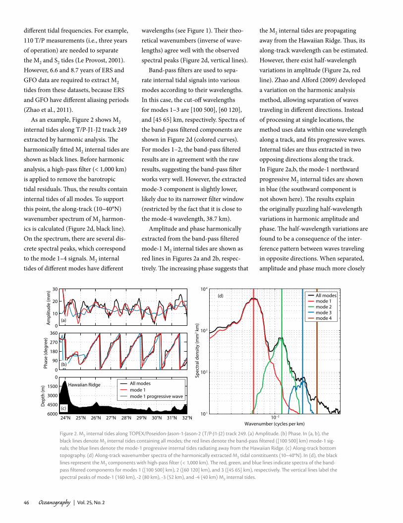
As an example, Figure 2 shows M2 internal tides along T/P-J1-J2 track 249 extracted by harmonic analysis. The harmonically fitted M2 internal tides are shown as black lines. Before harmonic analysis, a high-pass filter (< 1,000 km) is applied to remove the barotropic tidal residuals. Thus, the results contain internal tides of all modes. To support this point, the along-track (10–40°N) wavenumber spectrum of M2 harmon-ics is calculated (Figure 2d, black line). On the spectrum, there are several dis-crete spectral peaks, which correspond to the mode 1–4 signals. M2 internal tides of different modes have different

wavelengths (see Figure 1). Their theo-retical wavenumbers (inverse of wave-lengths) agree well with the observed spectral peaks (Figure 2d, vertical lines).

Band-pass filters are used to sepa-rate internal tidal signals into various modes according to their wavelengths. In this case, the cut-off wavelengths for modes 1–3 are [100 500], [60 120], and [45 65] km, respectively. Spectra of the band-pass filtered components are shown in Figure 2d (colored curves). For modes 1–2, the band-pass filtered results are in agreement with the raw results, suggesting the band-pass filter works very well. However, the extracted mode-3 component is slightly lower, likely due to its narrower filter window (restricted by the fact that it is close to the mode-4 wavelength, 38.7 km).

Amplitude and phase harmonically extracted from the band-pass filtered mode-1 M2 internal tides are shown as red lines in Figures 2a and 2b, respec-tively. The increasing phase suggests that

the M2 internal tides are propagating away from the Hawaiian Ridge. Thus, its along-track wavelength can be estimated. However, there exist half-wavelength variations in amplitude (Figure 2a, red line). Zhao and Alford (2009) developed a variation on the harmonic analysis method, allowing separation of waves traveling in different directions. Instead of processing at single locations, the method uses data within one wavelength along a track, and fits progressive waves. Internal tides are thus extracted in two opposing directions along the track. In Figure 2a,b, the mode-1 northward progressive M2 internal tides are shown in blue (the southward component is not shown here). The results explain the originally puzzling half-wavelength variations in harmonic amplitude and phase. The half-wavelength variations are found to be a consequence of the inter-ference pattern between waves traveling in opposite directions. When separated, amplitude and phase much more closely

0

10

20

30

Am

plitu

de (m

m)

(a)

0

90

180

270

360

Phas

e (d

egre

e)

(b)

24°N 25°N 26°N 27°N 28°N 29°N 30°N 31°N 32°N6000

4500

3000

1500

0

Dep

th (m

) Hawaiian Ridge

(c)

All modesmode 1mode 1 progressive wave

10–2101

102

103

104

Spec

tral

den

sity

(mm

2 km

)

Wavenumber (cycles per km)

(d) All modesmode 1mode 2mode 3mode 4

figure 2. M2 internal tides along Topex/poseidon-Jason-1-Jason-2 (T/p-J1-J2) track 249. (a) Amplitude. (b) phase. In (a, b), the black lines denote M2 internal tides containing all modes; the red lines denote the band-pass filtered ([100 500] km) mode-1 sig-nals; the blue lines denote the mode-1 progressive internal tides radiating away from the Hawaiian ridge. (c) Along-track bottom topography. (d) Along-track wavenumber spectra of the harmonically extracted M2 tidal constituents (10–40°N). In (d), the black lines represent the M2 components with high-pass filter (< 1,000 km). The red, green, and blue lines indicate spectra of the band-pass filtered components for modes 1 ([100 500] km), 2 ([60 120] km), and 3 ([45 65] km), respectively. The vertical lines label the spectral peaks of mode-1 (160 km), -2 (80 km), -3 (52 km), and -4 (40 km) M2 internal tides.

Oceanography | June 2012 47

resemble progressive waves. In Figure 2b, the northward-propagating mode-1 M2 internal tides show a clear linear phase increase and smoother amplitude, allow-ing better estimates of their energetics and propagation.

T Wo-dIMeNsIoNAL pL ANe-WAVe fITThe along-track analysis described above is a powerful tool for illustrating the existence of internal tidal waves that hap-pen to propagate nearly parallel to the satellite’s tracks. However, it is clearly of limited generality in an ocean with an arbitrary number of waves propagating in arbitrary directions. One proposed way forward has been to construct an inverse solution for a beam pattern based on a continuum of waves over a large area of ocean (Dushaw, 2002; Dushaw et al., 2011), but this approach ignores the spatial inhomogeneity of energy sources and sinks. Instead, Ray and Cartwright (2001) developed a local plane-wave fit technique using the altimeter grid over a small region—analogous to using a clus-ter of moorings as an antenna to detect propagating wave signals (Hendry, 1977; Zhao and D’Asaro, 2011). They then used this method to present the first altimetric map of the M2 internal tide around the Hawaiian Ridge. Zhao and Alford (2009) refined Ray and Cartwright’s (2001) method to resolve multiple waves.

The plane-wave fit technique uses the SSH measurements at all data points in one region from several neighboring ground tracks. In each radial direction, a single best-fit wave (amplitude and phase) can be determined. Its frequency is known (the tidal constituent, e.g., M2 or S2) and its wavelength is known from the baroclinic eigenvalue equa-tion (Equation 1), given a stratification profile, water depth, and latitude. When

the fitted amplitude is plotted versus compass direction, a wave appears as a lobe (Figure 3).

The plane-wave fit technique is lim-ited by the density of the satellite ground tracks relative to the internal tide wave-length (Ray and Cartwright, 2001). The fitting region must be big enough to con-tain several neighboring tracks as well as to span a significant fraction of the wave, but smaller fitting windows are better able to resolve structures in the internal tide field. In addition, the presence of multiple internal tides requires higher resolution to resolve the resultant com-plicated patterns. Multisatellite altimetry allows smaller fitting windows to be used. As Figure 3 shows, waves with win-dows smaller than 240 km on a side can-not be identified using data from a single altimeter, but with four sets of ground

tracks, waves can be separated with smaller fitting windows. Importantly, the fitted amplitudes in smaller fitting regions are also greater than those from bigger fitting regions. But there is a trade-off between spatial resolution and directional resolution (Zhao et al., 2011). As known from antenna theory, the smaller the fitting region, the poorer the angular resolution (Hendry, 1977).

Multiple internal tides may exist in one given region and cause complicated interference patterns (Rainville et al., 2010; Zhao et al., 2010). These waves must be resolved separately to inter-pret their propagation and energetics accurately (Alford and Zhao, 2007). The improved plane-wave fit technique may resolve multiple waves. For the location shown in Figure 3d, there are two out-standing lobes corresponding to the two

figure 3. An example of the plane-wave fit technique around 33.5°N, 199°e (black dots). (a) ground tracks of T/p-J1-J2 and T/pt-J1t (t = tandem). (b) ground tracks of T/p-J1-J2, T/pt-J1t, ers, and gfo. (c, d) radial ampli-tude of mode-1 M2 internal tides plotted versus direction, obtained using dif-ferent datasets in (a) and (b), respectively. The colored boxes in (a, b) denote the sizes of the fitting regions, and the colored curves in (c, d) denote the fitted amplitudes. In (d), the arrows indicate the northeastward and south-eastward Hawaiian and Aleutian beams. Adapted from Zhao et al. (2011)

60 120 180

30

210

60

240

90

270

120

300

150

330

180 0

(a)

60 120 180

30

210

60

240

90

270

120

300

150

330

180 0

(b)

T/P−J1−J2T/Pt−J1tERSGFO

6 12 18

30

210

60

240

90

270

120

300

150

330

180 0

unit: mm

(c)

6 12 18

30

60

240

90

270

120

300

150

330

180 0

unit: mm

(d)

120 km180 km240 km

Oceanography | Vol. 25, No. 248

internal tide beams originating from the Hawaiian and Aleutian ridges (see figure on page 44).

Due to the irregular distribution of ground tracks, some lobes may be arti-facts of the antenna rather than actual waves. The biggest of these “side lobes” in the multisatellite calculations may reach to 20% of the main wave (Zhao et al., 2011). To minimize the impact of the side lobes on the solutions for waves traveling in other directions, an iterative procedure is used (Figure 4). First, the amplitude, phase, and direction of the wave with the greatest amplitude are determined from the raw signals (Figure 4b, blue arrow). A plane wave with these parameters is then generated (blue curve) and subtracted from the raw data (green). This step has the effect of removing both the wave and its side lobes from the signals. The procedure can then be repeated for as

many waves as desired. In practice, only two or three waves generally dominate the signals (Figure 4c,d). Once these waves are determined, the entire proce-dure is repeated for each wave with the other waves subtracted (Figure 4, red, green, and brown arrows). This proce-dure improves the result because the side lobes of the other waves are removed while computing the solution for each wave. Note that the final computed waves (Figure 4f, colored arrows) differ slightly from the initial ones (black arrows).

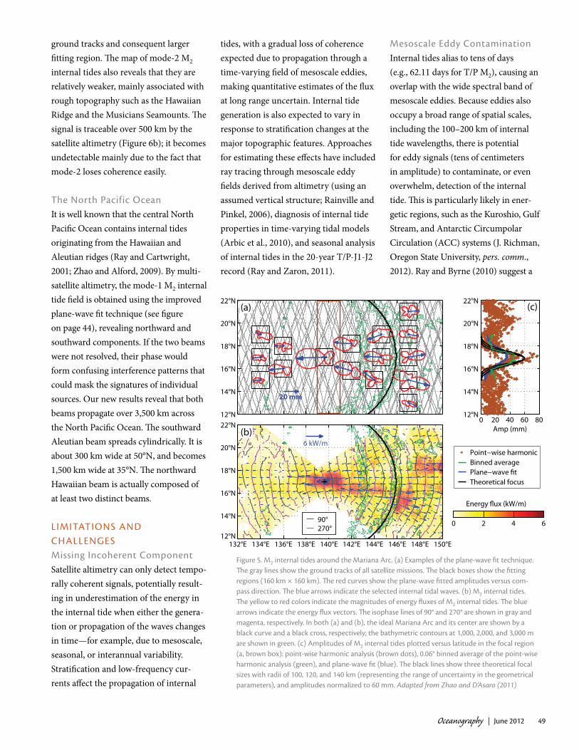
regIoNAL resuLTsMariana ArcThe Mariana Arc approximates an arc of a circle 630 km in radius centered at 17°N, 139.6°E (Figure 5, black curve). Examples of the plane-wave fit tech-nique are shown in 16 fitting windows of 160 km on a side (Zhao and D’Asaro,

2011; Figure 5a). The results reveal that internal tides are generally in the east–west direction. Note that previous stud-ies have focused mainly on internal tides in the south–north direction because they are closer to the track direction. This example confirms that the phase variation across multiple tracks allows for the robust extraction of eastward and westward waves.

The westward-propagating M2 inter-nal tides from the Mariana Arc con-verge at its center (Figure 5b). In the focal region centered at 17°N, 139.6°E, the spatially smoothed energy flux is about 6.5 kW m–1, about four times the along‐arc mean value, while the spatially unsmoothed energy flux may reach up to 17 kW m–1, comparable to the value at the Hawaiian Ridge (Zaron et al., 2009). M2 internal tides converge in a focal region of a size comparable to that of a perfect focus (Figure 5c).

Hawaiian ridgeA clear view of the M2 internal tides around the Hawaiian Ridge is provided by the high spatial resolution of multi-satellite altimetry (Zhao et al., 2011). The resultant mode-1 and -2 energy fluxes emanating from the Hawaiian Ridge are illustrated in Figure 6a and 6b, respectively. Discrete generation sites and internal tidal beams are distinguish-able. Previous studies could only discern three generation sites: Nihoa Island (NI), Kauai Channel (KC), and French Frigate Shoals (FFS); now, more generation sites are resolved. M2 internal tidal energy fluxes estimated from multisatellite altimetry products are greater and agree better with model results than previ-ous single satellite estimates (Ray and Cartwright, 2001). This agreement con-firms that previous underestimates were partly due to the more widely spaced

50

100

30

210

60

240

90

270

120

300

150

330

0081

(a)

5 10 15

30

210

60

240

90

270

120

300

150

330

0081

(b)

5

10

30

210

60

240

90

270

120

300

150

330

0081

(c)

2.5 5

30

210

60

240

90

270

120

300

150

330

0081

(d)

5 10 15

30

210

60

240

90

270

120

300

150

330

0081

(e)

5 10 15

30

210

60

240

90

270

120

300

150

330

0081

(f)

figure 4. Illustration of the iterative plane-wave fit technique using synthetic data. (a) data points within a 140 km window from a typical multiple satellite track pattern. Three M2 waves are cre-ated (black arrows). (b) Initially fitted amplitude (black) with the maximal lobe selected (blue arrow). The green line shows the fitted amplitude after removing the first wave (blue curve). (c) repeat (b) to determine and remove the second wave. (d) repeat (c) to determine and remove the third wave. The final residual is shown in black. (e) The three waves are readjusted by the plane-wave fit technique with the other two waves removed. The blue arrows denote these waves before the adjustment, while the red, green, and brown arrows denote waves after adjustment. (f) Comparisons of the real waves (black, from panel a) and the finally determined waves (colored).

Oceanography | June 2012 49

ground tracks and consequent larger fitting region. The map of mode-2 M2 internal tides also reveals that they are relatively weaker, mainly associated with rough topography such as the Hawaiian Ridge and the Musicians Seamounts. The signal is traceable over 500 km by the satellite altimetry (Figure 6b); it becomes undetectable mainly due to the fact that mode-2 loses coherence easily.

The North pacific oceanIt is well known that the central North Pacific Ocean contains internal tides originating from the Hawaiian and Aleutian ridges (Ray and Cartwright, 2001; Zhao and Alford, 2009). By multi- satellite altimetry, the mode-1 M2 internal tide field is obtained using the improved plane-wave fit technique (see figure on page 44), revealing northward and southward components. If the two beams were not resolved, their phase would form confusing interference patterns that could mask the signatures of individual sources. Our new results reveal that both beams propagate over 3,500 km across the North Pacific Ocean. The southward Aleutian beam spreads cylindrically. It is about 300 km wide at 50°N, and becomes 1,500 km wide at 35°N. The northward Hawaiian beam is actually composed of at least two distinct beams.

LIMITATIoNs ANd CHALLeNgesMissing Incoherent ComponentSatellite altimetry can only detect tempo-rally coherent signals, potentially result-ing in underestimation of the energy in the internal tide when either the genera-tion or propagation of the waves changes in time—for example, due to mesoscale, seasonal, or interannual variability. Stratification and low-frequency cur-rents affect the propagation of internal

tides, with a gradual loss of coherence expected due to propagation through a time-varying field of mesoscale eddies, making quantitative estimates of the flux at long range uncertain. Internal tide generation is also expected to vary in response to stratification changes at the major topographic features. Approaches for estimating these effects have included ray tracing through mesoscale eddy fields derived from altimetry (using an assumed vertical structure; Rainville and Pinkel, 2006), diagnosis of internal tide properties in time-varying tidal models (Arbic et al., 2010), and seasonal analysis of internal tides in the 20-year T/P-J1-J2 record (Ray and Zaron, 2011).

Mesoscale eddy ContaminationInternal tides alias to tens of days (e.g., 62.11 days for T/P M2), causing an overlap with the wide spectral band of mesoscale eddies. Because eddies also occupy a broad range of spatial scales, including the 100–200 km of internal tide wavelengths, there is potential for eddy signals (tens of centimeters in amplitude) to contaminate, or even overwhelm, detection of the internal tide. This is particularly likely in ener-getic regions, such as the Kuroshio, Gulf Stream, and Antarctic Circumpolar Circulation (ACC) systems (J. Richman, Oregon State University, pers. comm., 2012). Ray and Byrne (2010) suggest a

Energy �ux (kW/m)

0 2 4 6

6 kW/m(b)

132°E 134°E 136°E 138°E 140°E 142°E 144°E 146°E 148°E 150°E

12°N

14°N

16°N

18°N

20°N

22°N

12°N

14°N

16°N

18°N

20°N

22°N

12°N

14°N

16°N

18°N

20°N

22°N0 20 40 60 80

Amp (mm)

(c)

Point−wise harmonicBinned averagePlane−wave �tTheoretical focus

20 mm

(a)

90°270°

figure 5. M2 internal tides around the Mariana Arc. (a) examples of the plane-wave fit technique. The gray lines show the ground tracks of all satellite missions. The black boxes show the fitting regions (160 km × 160 km). The red curves show the plane-wave fitted amplitudes versus com-pass direction. The blue arrows indicate the selected internal tidal waves. (b) M2 internal tides. The yellow to red colors indicate the magnitudes of energy fluxes of M2 internal tides. The blue arrows indicate the energy flux vectors. The isophase lines of 90° and 270° are shown in gray and magenta, respectively. In both (a) and (b), the ideal Mariana Arc and its center are shown by a black curve and a black cross, respectively; the bathymetric contours at 1,000, 2,000, and 3,000 m are shown in green. (c) Amplitudes of M2 internal tides plotted versus latitude in the focal region (a, brown box): point-wise harmonic analysis (brown dots), 0.06° binned average of the point-wise harmonic analysis (green), and plane-wave fit (blue). The black lines show three theoretical focal sizes with radii of 100, 120, and 140 km (representing the range of uncertainty in the geometrical parameters), and amplitudes normalized to 60 mm. Adapted from Zhao and D’Asaro (2011)

Oceanography | Vol. 25, No. 250

cure for this contamination through the use of the “other” multisatellite product: the time-averaged and gridded AVISO maps of mesoscale SSH. By subtracting these maps prior to harmonic analysis for internal tides, they make use of the anti-aliasing aspects of multisatellite altime-try: while aliased internal tides may con-taminate some aspects of the mesoscale maps, the smoothing over multiple tracks removes the time-coherent signal present in each altimeter. They report that this method works well in the ACC region off South Africa, setting the stage for its use in other energetic regions.

perspeC TIVeAssimilation to Numerical ModelsIncreasing computational power is approaching the capability to simulate the global internal tide field (Simmons et al., 2004; Arbic et al., 2010; Egbert et al., 2012). Field measurements for the validation of these models are scarce and sometimes hard to interpret due to complex interference patterns, making altimetric results a key component of

future modeling efforts. Though satel-lite altimetry may underestimate their amplitude, the phase of internal tides is very well defined (see Figure 10 in Zhao et al., 2011) and may be a robust bench-mark for models.

sWoT satellite AltimetryDirect observations of internal tides will receive a huge boost from the Surface Water and Ocean Topography (SWOT) wide-swath altimeter, which will pro-vide real two-dimensional observations of SSH at ~ 5 km spatial resolution, far superior to the current neighbor-ing ground tracks of multiple satellites (Fu et al., 2010). The planned accuracy is expected to allow the detection of significantly smaller-scale high-mode components than the first four described here and will enable an unprecedented view of the internal tide generation and dissipation sites. With a 100 km wide swath, average revisit times will depend on latitude, with two to four revisits at low to mid latitudes and up to 10 revis-its at high latitudes per ~ 20 day repeat

period (Fu et al., 2010; Durand et al., 2010). These revisits may help loosen the limitations of harmonic analysis, but several years of data accumulation will still be required before internal tides can be extracted.

ACKNoWLedgMeNTsZ. Zhao and M.H. Alford were sup-ported by NSF grants OCE-1029268 and OCE-1129129. J.B. Girton was supported by ONR grant N00014-08-1-0983. The altimeter products were produced by Ssalto/Duacs and distributed by AVISO, with support from CNES (http://www.aviso.oceanobs.com/duacs).

refereNCesAlford, M.H. 2003. Redistribution of energy avail-

able for ocean mixing by long-range propaga-tion of internal waves. Nature 423:159–162, http://dx.doi.org/10.1038/nature01628.

Alford, H.M., J. MacKinnon, Z. Zhao, R. Pinkel, and T. Peacock. 2007. Internal waves across the Pacific. Geophysical Research Letters 37, L24061, http://dx.doi.org/10.1029/2007GL031566.

Alford, M.H., and Z. Zhao. 2007. Global pat-terns of low-mode internal-wave propaga-tion. Part II: Group velocity. Journal of Physical Oceanography 37:1,849–1,858, http://dx.doi.org/10.1175/JPO3086.1.

180°W 176°W 172°W 168°W 164°W 160°W 156°W 152°W 180°W 176°W 172°W 168°W 164°W 160°W 156°W 152°W12°N

14°N

16°N

18°N

20°N

22°N

24°N

26°N

28°N

30°N

32°N

34°N

8 kW/m

4 kW/m

(a) Energy �ux of the M2 internal tide: Mode 1

KCNI

FFS

MI

LiI LaI GP

Line Islands Ridge

Musicians Seam

ounts

Necker Ridge

Mid−Paci�cMountains

1 kW/m

0.5 kW/m

(b) Energy ux of the M2 internal tide: Mode 2

KCNI

FFS

MI

LiI LaI GP

Line Islands Ridge

Musicians Seam

ounts

Necker Ridge

Mid−Paci�cMountains

figure 6. (a) energy flux of mode-1 M2 internal tides around the Hawaiian ridge, estimated from multisatellite altimetry using a 120 km fitting region. The 4,000 m isobath contours are shown in gray. remarkable generation sites are labeled: Midway Island (MI), Lisianski Island (LiI), Laysan Island (LaI), gardner pinnacles (gp), french frigate shoals (ffs), Nihoa Island (NI), and Kauai Channel (KC). red and green arrows indicate southward and northward internal tides, respectively. flux arrows smaller than 0.15 kW m–1 are not plotted. (b) Mode-2 M2 internal tides. flux arrows smaller than 0.05 kW m–1 are not plotted. Adapted from Zhao et al. (2011)

Oceanography | June 2012 51

Arbic, B.K., A.J. Wallcraft, and E.J. Metzger. 2010. Concurrent simulation of the eddying general circulation and tides in a global ocean model. Ocean Modelling 32:175–187, http://dx.doi.org/ 10.1016/j.ocemod.2010.01.007.

Chiswell, S.M. 2006. Altimeter and cur-rent meter observations of internal tides: Do they agree? Journal of Physical Oceanography 36:1,860–1,872, http://dx.doi.org/10.1175/JPO2944.1.

Colosi, J.A., and W. Munk. 2006. Tales of the vener-able Honolulu tide gauge. Journal of Physical Oceanography 36:967–996, http://dx.doi.org/ 10.1175/JPO2876.1.

Cummins, P.F., J.Y. Cherniawsky, and M.G.G. Foreman. 2001. North Pacific inter-nal tides from the Aleutian Ridge: Altimeter observations and modeling. Journal of Marine Research 59:167–191.

Dale, A.C., J.M. Huthnance, and T.J. Sherwin. 2001. Coastally-trapped waves and tides at near-inertial frequencies. Journal of Physical Oceanography 31:2,958–2,970, http://dx.doi.org/10.1175/1520-0485(2001)031 <2958:CTWATA>2.0.CO;2.

Durand, M., L.L. Fu, D.P. Lettenmaier, D.E. Alsdorf, E. Rodriguez, and D. Esteban-Fernandez. 2010. The surface water and ocean topography mission: Observing terrestrial surface water and oceanic submesoscale eddies. Proceedings of the IEEE 98:766–779, http://dx.doi.org/10.1109/JPROC.2010.2043031.

Dushaw, B.D. 2002. Mapping low-mode internal tides near Hawaii using TOPEX/POSEIDON altimeter data. Geophysical Research Letters 29, 1250, http://dx.doi.org/10.1029/2001GL013944.

Dushaw, B.D. 2006. Mode-1 internal tides in the western North Atlantic Ocean. Deep-Sea Research Part I 53:449–473, http://dx.doi.org/ 10.1016/j.dsr.2005.12.009.

Dushaw, B.D., B.M. Howe, B.D. Cornuelle, P.F. Worcester, and D.S. Luther. 1995. Barotropic and baroclinic tides in the central North Pacific Ocean determined from long-range recipro-cal acoustic transmissions. Journal of Physical Oceanography 25:631–647, http://dx.doi.org/ 10.1175/1520-0485(1995)025<0631:BABTIT>2.0.CO;2.

Dushaw, B.D., P.F. Worcester, and M.A. Dzieciuch. 2011. On the predictability of mode-1 internal tides. Deep-Sea Research Part I 58(6):677–698, http://dx.doi.org/10.1016/j.dsr.2011.04.002.

Egbert, G.D., S.Y. Erofeeva, and E.D. Zaron. 2012. Mapping M2 internal tides using a data-assimilative reduced gravity model. Paper pre-sented at the Ocean Sciences Meeting, Salt Lake City, Utah, February 19, 2012, poster B2112.

Egbert, G.D., and R.D. Ray. 2000. Significant dissipation of tidal energy in the deep ocean inferred from satellite altimeter data. Nature 405:775–778, http://dx.doi.org/ 10.1038/35015531.

Egbert, G.D., and R.D. Ray. 2001. Estimates of M2 tidal energy dissipation from TOPEX/Poseidon altimeter data. Journal of Geophysical Research 106(C10):22,475–22,502, http://dx.doi.org/10.1029/2000JC000699.

Fu, L.-L., D.B. Chelton, P.-Y. Le Traon, and R. Morrow. 2010. Eddy dynamics from satellite altimetry. Oceanography 23(4):14–25, http://dx.doi.org/10.5670/oceanog.2010.02.

Gill, A.E. 1982. Atmosphere-Ocean Dynamics. Academic Press, 662 pp.

Hendry, R.M. 1977. Observations of the semidiur-nal internal tide in the western North Atlantic Ocean. Philosophical Transactions of the Royal Society of London A 286:1–26, http://dx.doi.org/ 10.1098/rsta.1977.0108.

Kantha, L.H., and C.C. Tierney. 1997. Global baroclinic tides. Progress in Oceanography 40:163–178, http://dx.doi.org/ 10.1016/S0079-6611(97)00028-1.

Kunze, E., and S.G. Llewellyn Smith. 2004. The role of small-scale topography in turbulent mixing of the global ocean. Oceanography 17(1):55–64, http://dx.doi.org/10.5670/oceanog.2004.67.

MacKinnon, J.A., and K.B. Winters. 2005. Subtropical catastrophe: Significant loss of low-mode tidal energy at 28.9. Geophysical Research Letters 32, L15605, http://dx.doi.org/ 10.1029/2005GL023376.

Maraldi, C., F. Lyard, L. Testut, and R. Coleman. 2011. Energetics of internal tides around the Kerguelen Plateau from modeling and altimetry. Journal of Geophysical Research 116, C06004, http://dx.doi.org/10.1029/2010JC006515.

Le Provost, C. 2001. Ocean tides. Pp. 267–303 in Satellite Altimetry and Earth Sciences: A Handbook for Technique and Applications. L.-L. Fu and A. Cazenave, eds, Academic, San Diego, California.

Munk, W.H., and D.C. Cartwright. 1966. Tidal spectroscopy and prediction. Philosophical Transactions of the Royal Society of London A 259:533–581, http://dx.doi.org/ 10.1098/rsta.1966.0024.

Munk, W.H., and C. Wunsch. 1998. Abyssal recipes II: Energetics of tidal and wind mixing. Deep-Sea Research Part I 45:1,977–2,010, http://dx.doi.org/10.1016/S0967-0637(98)00070-3.

Nash, J.D., M.H. Alford, E. Kunze, K. Martini, and S. Kelly. 2007. Hotspots of deep ocean mixing on the Oregon continental slope. Geophysical Research Letters 34, L01605, http://dx.doi.org/ 10.1029/2006GL028170.

Rainville, L., T.M.S. Johnston, G.S. Carter, M.A. Merrifield, R. Pinkel, P.F. Worcester, and B.D. Dushaw. 2010. Interference pat-tern and propagation of the M2 internal tide south of the Hawaiian Ridge. Journal of Physical Oceanography 40:311–325, http://dx.doi.org/10.1175/2009JPO4256.1.

Rainville, L., and R. Pinkel. 2006. Propagation of low-mode internal waves through the ocean. Journal of Physical Oceanography 36:1,220–1,236, http://dx.doi.org/10.1175/JPO2889.1.

Ray, R.D., and D.A. Byrne. 2010. Bottom pres-sure tides along a line in the southeast Atlantic Ocean and comparisons with satellite altim-etry. Ocean Dynamics 60:1,167–1,176, http://dx.doi.org/10.1007/s10236-010-0316-0.

Ray, R.D., and D.E. Cartwright. 2001. Estimates of internal tide energy fluxes from TOPEX/Poseidon altimetry: Central North Pacific. Geophysical Research Letters 28:1,259–1,262, http://dx.doi.org/10.1029/2000GL012447.

Ray, R.D., G.D. Egbert, and S.Y. Erofeeva. 2011. Tide predictions in shelf and coastal waters: Status and prospects. Pp. 191–216 in Coastal Altimetry. S. Vignudelli, A.G. Kostianoy, P. Cipollini, and J. Benveniste, eds, Springer, New York.

Ray, R.D., and G.T. Mitchum. 1996. Surface manifestation of internal tides gener-ated near Hawaii. Geophysical Research Letters 23:2,101–2,104, http://dx.doi.org/ 10.1029/96GL02050.

Ray, R.D., and G.T. Mitchum. 1997. Surface mani-festation of internal tides in the deep ocean: Observations from altimetry and island gauges. Progress in Oceanography 40:135–162, http://dx.doi.org/10.1016/S0079-6611(97)00025-6.

Ray, R.D., and E.D. Zaron. 2011. Non-stationary internal tides observed with satellite altimetry. Geophysical Research Letters 38, L17609, http://dx.doi.org/10.1029/2011GL048617.

Simmons, H.L, R.W. Hallberg, and B.K. Arbic. 2004. Internal wave generation in a global baroclinic tide model. Deep-Sea Research Part II 51:3,043–3,068, http://dx.doi.org/ 10.1016/j.dsr2.2004.09.015.

St. Laurent, L., and C. Garrett. 2002. The role of internal tides in mixing the deep ocean. Journal of Physical Oceanography 32:2,882–2,899, http://dx.doi.org/10.1175/1520-0485(2002) 032<2882:TROITI>2.0.CO;2.

Tian, J., L. Zhou, and X. Zhang. 2006. Latitudinal distribution of mixing rate caused by the M2 internal tide. Journal of Physical Oceanography 36:35–42, http://dx.doi.org/ 10.1175/JPO2824.1.

Wunsch, C. 1975. Internal tides in the ocean. Reviews of Geophysics 13:167–182, http://dx.doi.org/10.1029/RG013i001p00167.

Zaron, E.D., C. Chavanne, G.D. Egbert, and P. Flament. 2009. Baroclinic tidal gen-eration in the Kauai Channel inferred from high-frequency radio Doppler cur-rent meters. Dynamics of Atmospheres and Oceans 48(1–3):93–120, http://dx.doi.org/ 10.1016/j.dynatmoce.2009.03.002.

Zhao, Z., and M.H. Alford. 2009. New altimet-ric estimates of mode-1 M2 internal tides in the central North Pacific Ocean. Journal of Physical Oceanography 39:1,669–1,684, http://dx.doi.org/10.1175/2009JPO3922.1.

Zhao, Z., M.H. Alford, J. Girton, T.M.S. Johnston, and G.S. Carter. 2011. Internal tides around the Hawaiian Ridge estimated from multi-satelliate altimetry. Journal of Geophysical Research 41, JC12041, http://dx.doi.org/ 10.1029/2011JC007045.

Zhao, Z., M.H. Alford, J.A. MacKinnon, and R. Pinkel. 2010. Long-range propaga-tion of the semidiurnal internal tides from the Hawaiian Ridge. Journal of Physical Oceanography 40:713–736, http://dx.doi.org/ 10.1175/2009JPO4207.1.

Zhao, Z., and E.A. D’Asaro. 2011. A perfect focus of the internal tide from the Mariana Arc. Geophysical Research Letters 38, L14609, http://dx.doi.org/10.1029/2011GL047909.