OCCUPATIONAL SEGREGATION AND THE GENDER WAGE … · Economia Aplicada, v. 14, n. 2, 2010, pp....

Economia Aplicada, v. 14, n. 2, 2010, pp. 147-168

OCCUPATIONAL SEGREGATION AND THE GENDERWAGE GAP IN BRAZIL: AN EMPIRICAL ANALYSIS*

Regina Madalozzo †

Abstract

Several countries experienced an increase in female labor participa-tion during the twentieth century. Even so, few can be proud of the con-ditions female workers faced. This paper analyzes the occupational dis-tribution by gender from 1978 to in 2007 in Brazil. It shows that womenhave penetrated traditionally male occupations to a certain extent, butthat traditionally female occupations have maintained their gender com-position over the past 30 years. We also provide a regression analysis withan Oaxaca decomposition that shows that the gender wage gap is lowerthan in 1978, but that it has remained constant over the last decade.

Keywords: wage differentials, discrimination, and female labor market.

Palavras-chave: diferenciais de salário, discriminação, mercado de traba-lho feminino

JEL classification: J24, J31, J71.

1 Introduction

Virtually all countries experienced an increase in female labor participationduring the twentieth century. Even so, few can be proud of the conditions thatfemale workers face in dealing with family responsibilities and the labor mar-ket. The division of labor within families continues to fall along traditionalgender lines, even when women engage in labor market activities. Womenwho are engaged in the labor market are still expected to be available to com-ply with their family responsibilities of housework, childcare and other activi-ties (Hersch & Stratton 1994, Alvarez et al. 2006, Lundberg 2008, Madalozzoet al. 2008, Gupta & Ash 2008). Further, women continue to receive lowerwages than men, even when controlling for personal characteristics and jobattributes (Blau & Kahn 1997, Bertrand & Hallock 2001, Albrecht et al. 2003,Bayard et al. 2003, Bucheli & Sanroman 2005, Galarza et al. 2006, Madalozzo& Martins 2007, Olivetti & Petrongolo 2008). There is no consensus amongspecialists as to whether a gendered division of labor at home causes the wagegap or vice versa. However, the majority of studies agree that some intrinsic

* This paper has benefited from the suggestions made by an anonymous referee and the excellentresearch assistance of Carolina Flores Gomes. The research was conducted with financial supportfrom CNPq (Productivity Research Fellowship #307513/2007-6)† Insper Instituto de Ensino e Pesquisa, email:[email protected]

Recebido em 10 de março de 2009 . Aceito em 10 de fevereiro de 2010.

148 Regina Madalozzo Economia Aplicada, v.14, n.2

features of gender have a significant influence on these outcomes of a lowerwage and second shift.

One possibility is that the career interruptions that women experience dur-ing their reproductive life1 make them less productive on the labor marketand, therefore, available to work for lower wage rates (Deloach & Hoffman2002, Hersch & Stratton 2002, Moe 2003, Blau et al. 2006, Bryan & Sanz2007). Another possibility is that women’s wages are lower because they ac-count for benefits that are available only to women, for example, maternityleave (Waldfogel 1998, Edwards 2006, Bergmann 2008). As a final point, an-other possibility is that women choose to work in occupations and activitieswith lower remuneration than those chosen by men (Easterlin 1995, Macpher-son & Hirsch 1995, Miller 2009). Any of these possibilities may impact – orbe impacted by – the gender division of labor by making it less costly to thehousehold for women to spend more hours at home instead of men; if bothspouses are equally productive to the market, but the husband receives higherremuneration for his work than his wife, he has a comparative advantage indedicating more time and effort to the market (Ferber 2003).

Our focus in this study is to analyze female labor participation in Brazilsince the 1970s. Brazil is a highly unequal country in several aspects. It hasone of the worst Gini indexes in the world, 0.567, and had the 10th worst in-come distribution in the world in 2007. Concerning gender differences, Brazilranked 74th out of 127 countries in the 2007World Economic Forum’s GenderGap index, with a score of 0.664.2 Using data from 1978 to 2007 will allow usto understand two different problems related to women’s labor participation:occupational segregation and the gender wage gap over time.

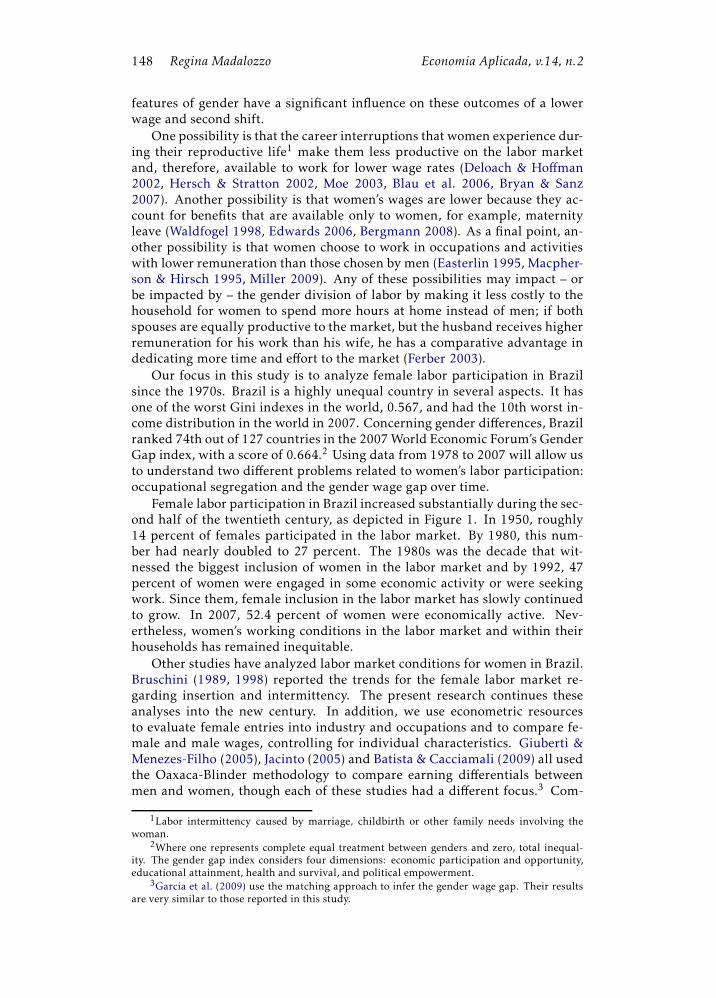
Female labor participation in Brazil increased substantially during the sec-ond half of the twentieth century, as depicted in Figure 1. In 1950, roughly14 percent of females participated in the labor market. By 1980, this num-ber had nearly doubled to 27 percent. The 1980s was the decade that wit-nessed the biggest inclusion of women in the labor market and by 1992, 47percent of women were engaged in some economic activity or were seekingwork. Since them, female inclusion in the labor market has slowly continuedto grow. In 2007, 52.4 percent of women were economically active. Nev-ertheless, women’s working conditions in the labor market and within theirhouseholds has remained inequitable.

Other studies have analyzed labor market conditions for women in Brazil.Bruschini (1989, 1998) reported the trends for the female labor market re-garding insertion and intermittency. The present research continues theseanalyses into the new century. In addition, we use econometric resourcesto evaluate female entries into industry and occupations and to compare fe-male and male wages, controlling for individual characteristics. Giuberti &Menezes-Filho (2005), Jacinto (2005) and Batista & Cacciamali (2009) all usedthe Oaxaca-Blinder methodology to compare earning differentials betweenmen and women, though each of these studies had a different focus.3 Com-

1Labor intermittency caused by marriage, childbirth or other family needs involving thewoman.

2Where one represents complete equal treatment between genders and zero, total inequal-ity. The gender gap index considers four dimensions: economic participation and opportunity,educational attainment, health and survival, and political empowerment.

3Garcia et al. (2009) use the matching approach to infer the gender wage gap. Their resultsare very similar to those reported in this study.

Occupational Segregation 149

0

10

20

30

40

50

60

70

80

90

100

1950 1960 1970 1980 1990 2000female male

Source: IBGE, Estatísticas do Século XX

Figure 1: Labor Market Participation. Male and Female, 1950–2007.

plementing their work, we expanded the period analyzed and emphasized therole of occupation choice in wage profiles. Our analyses target the average dif-ferences in labor market earnings for men and women for the period between1978 and 2007. Finally, Scorzafave & Pazello (2007) also studied the genderwage gap in Brazil, however their goal was to apply normalized equations tosolve the indetermination problem of the Oaxaca-Blinder decomposition ap-proach. We use their methodology in our research to better understand theimpact of the occupation transition process on narrowing the gender wagegap during this period.4

This paper is organized as follows: in the next section we describe Brazil-ian labor characteristics, focusing on activities and gender differentials. Sec-tion 3 explains the empirical model used to analyze the gender gap in remu-neration and the impact of occupational differentials. The results are pre-sented in Section 4. Section 5 offers conclusions.

2 The Brazilian labor market: are there gender differences?

In this section, we describe Brazilian labor markets and highlight the differ-ences and similarities between genders with regard to them. Before enteringinto such a discussion, however, it is necessary to explain some peculiaritiesof the Brazilian labor market. First, it is highly regulated. Since the 1930s,with the implementation of the first laws concerning employment in Brazil,there have been an increased number of restrictions and fees employers mustpay to be able to hire individuals. The constitution of 1988 aggravated thisproblem. Second, women have gained specific rights to maternity leave. Be-fore 1988, all female workers had the right to a fully paid maternity leaveof 90 days. The new constitution increased this right to 120 days. In 2007,

4By no means do these cited studies cover the entire body of literature on the gender wagegap in Brazil. However, the studies presented here are closely related to the goals and methodsof this paper.


new federal legislation was passed in response to the World Health Organiza-tion’s recommendation that babies should be breastfed for 6 months. Underthis law, female workers may opt to take 6 months of maternity leave, alsofully paid by the employer.5 These stringent regulations on the labor marketare the concern of many researchers, who question their ability to guaranteeworkers’ rights by suggesting that such regulations may force workers intoinformal jobs, where they will have no rights at all.

Our analysis used microdata from PNAD (Pesquisa Nacional de Amostrapor Domicílios, which translates to National Survey of Sampled Households).PNAD is an annual survey conducted by the Brazilian Bureau of Statistics,IBGE. It takes a representative sample of Brazilian households and studies,among other aspects of the population, labor, education and health. It con-tains data at an individual level for the sampled dwellings. Since 2004, PNADhas investigated data for all national territory.6 With the purpose of analyz-ing the past and current employment trends, we used data from four differentdecades: 1978, 1988, 1998, and 2007, the most recent data released by IBGE.Questionnaires were modified during this period; however, we made someconcatenations in order to make them comparable.

Table 1 presents the female distribution among different occupation cat-egories.7 For each year, we divided the occupations into traditionally maleor traditionally female.8 It can be observed that the majority of occupa-tions remain majority male over time (for example, carpenters, mechanics,drivers, etc.), while others maintain their tendency to be female-dominatedoccupations (including nurses, librarians, and schoolteachers). Nevertheless,some changes are visible. While in 1978 only 4.94 percent of engineers werewomen, in 2007 more than 10 percent of engineers were female. This is stilla small number of individuals; however, it establishes a change in pattern.Other examples of traditionally male occupations that are being occupied byincreasing numbers women are insurance agents, police and detectives, andmanagers and administrators.

On the other side, traditionally female occupations rarely present such achange. There are a few possible explanations for this phenomenon. The firstis that men resist engaging in activities that are regarded as “female.” Thiswould reflect gender preferences for certain activities and against others. His-torically, women engaged in market activities closely related to their domesticwork (Folbre 1994). Considering that men have historically been distant fromsuch work, it is plausible to infer that males would prefer a different typeof activity and, therefore, favor traditionally male occupations.It may also bethe case that this difference is related to worker discrimination (Kaufman &Hotchkiss 2003). This would be the case if men charged a premium to work

5Up to a ceiling of 12 thousand Reais, maternity leave is paid by the employer who is reim-bursed by the government in taxes. This is a very high ceiling. Less than 3 percent of femaleworkers earn more than this value monthly.

6Until then, 1.9 percent of the Brazilian population was not included in the sample becausethey lived in areas not researched. However, the analysis contains weights that allow for compar-ison with earlier years.

7This table was inspired by Table 8.3, in Kaufman & Hotchkiss (2003, p.425).8It may be pointed out that there is a very high level variation in the number of individuals

in some categories. For instance, the number of individuals that claim to be economists in 2007is well above the expected increase in the population. However, the result is conditional on theindividual weight assigned to the population. Even when the weight is corrected for individualcharacteristics, it may still distort individual data, such as occupation.


Table 1: Percentage of females in traditionally male and traditionally femaleoccupations.

Traditionally Male Occupations

Occupation 1978 1988 1998 2007

Engineers 4.94[4,778]

2.47[455]

8.35[15,682]

10.08[29,382]

Lawyers 18.18[15,386]

25.86[3,708]

38.40[104,003]

43.86[207,225]

Physicians 18.29[14,144]

22.07[4,285]

48.15[106,848]

42.87[96,607]

Economists 18.76[3,864]

16.84[665]

32.44[13,451]

76.13[228,013]

Clergy 20.54[5,249]

14.25[1,060]

27.79[24,984]

24.96[33,676]

Insurance agents 10.46[2,424]

0.00[0]

28.69[14,625]

32.69[32,178]

Managers and administrators 16.77[92,505]

17.10[26,282]

28.59[295,689]

36.48[1,609,614]

Carpenters 1.05[2,011]

0.28[207]

2.20[13,349]

2.04[8,108]

Auto mechanics 0.29[1,110]

1.19[1,132]

0.47[3,351]

1.36[9,286]

Telephone line installers 0.76[195]

0.00[0]

6.28[1,620]

3.05[3,393]

Drivers 0.17[2,070]

0.40[895]

1.20[25,395]

1.59[39,580]

Police and Detectives 2.28[1,746]

11.86[1,348]

11.71[17,188]

12.23[27,822]

Traditionally Female Occupations

Occupation 1978 1988 1998 2007

Registered nurses 86.94[247,258]

89.92[40,139]

86.83[59,379]

86.48[87,428]

Librarians 89.56[14,847]

82.10[3,595]

92.55[14,769]

79.41[4,259]

Schoolteachers 90.58[796,709]

88.87[88,539]

91.41[1,261,264]

81.54[1,942,572]

Bank tellers 54.70[119,922]

72.43[38,834]

51.94[115,502]

55.51[49,831]

Secretaries 52.23[944,816]

98.26[36,688]

61.48[194,194]

62.39[1,362,068]

Typists 37.04[56,654]

26.25[2,699]

91.82[372,472]

13.40[6,007]

Sewing machine operators 95.17[844,866]

97.00[144,360]

93.54[1,200,793]

91.99[1,213,158]

Dental assistants 22.53[10,467]

22.87[2,303]

53.49[56,295]

55.27[90,547]

Child care workers − 100.00[6,739]

97.86[407,142]

97.76[305,128]

Source: PNADs and author’s tabulation.All estimations are weighted by the individual weight available in the database.(Between squared brackets is the number of observations in the sample, using theappropriate weight.


with women in a “female job.” In that case, the premium could be so highthat firm owners prefer to hire only women because they are less costly. An-other alternative is that society resists having men in these occupations. Forexample, male nurses may be less socially desirable than female nurses. Aman who chooses to become a nurse may be viewed as a “failed doctor” moreeasily than a woman.9 This explanation is commonly known as “consumerprejudice” (Patterson & Engelberg 1978).

These differences in occupations and industry choices may be determi-nants of the remuneration discrepancy between genders. In order to bettercontrol this effect, Table 2 provides the individuals’ hourly pay by occupationand gender10 for 1978 and 2007. Table 3 does the same for economic sectorand gender.

Using the same categories analyzed in Table 1, it can be seen that, in mostcases, men have higher salaries than women. In 1978, for only two occupa-tions, drivers and librarians, did females have a higher average salary thanmales. For another 16 occupations, men received higher remuneration thanwomen. In 2007, the situation is slightly different: in 12 occupations, menearn greater wages than women and, for three others, women earn higherwages than men (auto mechanics, drivers, and police and detectives). Withno controls for education and industry, which we examine in the next section,it appears that there has been little change in the gender wage gap over a longperiod of time.

Concerning industry sectors, Table 3 shows that men typically receivedhigher wages than women in the past. However, in one activity, women’ssalaries are higher: construction. This is also one of the activities with lowerfemale engagement. One possible explanation for this premium on femalewages is individual selection. In order to participate in this industry, womenhave to be so different from the average that they receive higher wages thanmen. Analyzing the education distribution among industries, it can be seenthat in the construction industry women are more educated than men. In1978, almost 60 percent of females in the construction industry had 9 or moreyears of education (completed the primary level of education), while less than8 percent of males in this industry had this level of education. In 2007, 68percent of women in this industry had more than 9 years of education, while21 percent of men were in the same condition.

This question raises the importance of analyzing the degree of education.Comparing 1978 and 2007 data, we can see some different trends by genderin Table 4. In 1978, men with a low level of education were concentrated inthe agribusiness sector. Women with no education were also in agribusiness,but those who had a small amount of education (1 to 4 years) were in services.Men who had 5 to 11 years of education were in the transformation indus-try, while women at this level were generally in the services and the socialsector. Individuals of both genders with more than 11 years of education aremore concentrated in the social sector. The picture in 2007 is a little differ-ent. Men with low education levels continue to work in agribusiness (until 4years of education), and women in services. However, after finishing the basic

9Anecdotal evidence of this can be seen in the Hollywood hit movie “Meet the Parents,”where the parents of the fiancée avoid saying that their future son-in-law is a nurse.

10Here we do not control for hours of work or qualification (education degree, for example).These additional controls and others will be the focus of the next sections, with the regressionmodel.


Table 2: Hourly wage by gender and occupation: 1978 and 2007.

1978 2007

Occupation Men Women Men Women

Engineers 178.55[513]

158.88[23]

∗ 31.00[476]

22.45[64]

Lawyers 206.96[397]

135.82[103]

∗ 22.84[515]

19.32[384]

∗

Physicians 263.65[383]

125.52[96]

∗ 51.23[260]

35.15[196]

∗

Economists 246.08[117]

130.70[38]

∗ 23.29[136]

14.74[467]

∗

Clergy 34.85[100]

14.40[24]

∗ 7.22[217]

3.99[75]

∗

Insurance agents 69.06[122]

80.63[13]

13.51[110]

11.89[49]

Managers and administrators 99.08[2,546]

70.11[618]

∗ 17.97[5534]

15.34[3294]

∗

Carpenters 21.69[931]

8.56[8]

∗ 4.36[814]

2.26[15]

∗

Auto mechanics 24.04[1,768]

10.70[4]

∗ 4.95[1382]

8.30[21]

∗

Telephone line installers 34.54[140]

19.79[1]

∗ 5.36[200]

4.64[4]

∗

Drivers 27.13[5,549]

38.04[11]

∗ 6.36[4831]

8.42[75]

∗

Police and Detectives 52.64[440]

43.43[12]

∗ 12.47[448]

15.44[53]

∗

Registered nurses 31.38[190]

22.76[1322]

12.40[24]

12.76[177]

Librarians 26.60[8]

51.22[97]

∗ 91.61[2]

11.86[10]

Schoolteachers 55.65[429]

33.31[4174]

∗ 9.87[932]

8.75[3882]

∗

Bank tellers 51.43[531]

22.36[635]

∗ 12.48[70]

9.02[72]

∗

Secretaries 32.70[4,694]

29.56[5251]

∗ 7.43[1715]

5.93[2764]

∗

Typists 28.00[553]

22.12[394]

∗ 8.01[70]

2.81[11]

∗

Sewing machine operators 30.26[213]

12.57[4090]

∗ 3.29[212]

3.25[2495]

Dental assistants 192.14[214]

133.04[69]

∗ 23.58[138]

21.64[169]

Child care workers 6.79[18]

7.00[564]

Source: PNADs and author’s tabulation.All estimations are weighted by the individual weight available in the database.

* Indicates that the female and male values are different at 95% confidence intervalBetween square brackets is the number of observations in the sample, using theappropriate weight


Table 3: Hourly wage by gender and industries: 1978 and 2007.

1978 2007

Activity Men Women Men Women

Agricultural 14.86 6.49∗ 3.10 0.91∗

Transformation Industry 38.11 17.42∗ 7.12 4.33∗

Construction 23.21 38.82∗ 4.72 19.72∗

General Industry 31.46 33.10 10.45 11.02Commerce 38.26 21.81∗ 6.48 4.83∗

Services 40.00 12.30∗ 7.65 3.56∗

Transportation 32.67 26.39∗ 7.28 7.45Social Services 74.35 32.77∗ 13.45 8.26∗

Public Administration 50.08 45.15∗ 12.02 10.99∗

Other Activities 78.14 38.85∗ 9.12 7.04∗

Source: PNADs and author’s tabulation.All estimations are weighted by the individual weight available in thedatabase.∗ female and male values are different at the 95 percent confidence interval.

level of education, i.e., 4 years, men are employed in commerce. Women, fortheir part, continue to be concentrated in services until completing the fun-damental level of education, i.e., 8 years, and after that, they compose a largerfraction of commerce.

3 Econometric model to calculate discrimination betweengenders

The previous analysis illustrates that male and female workers have differentallocations within and returns to the labor market in Brazil. We now presentan econometric analysis in order to control for distinct influences on individ-ual remuneration. Using this procedure, we will also be able to measure theimpact of occupational choices and individual characteristics on the hourlywage.

The basic model follows Mincer (1995). The mincerian equation relatesthe hourly wage with individual demographics and job definitions, as shownby equation (1).

lnwi = α +k

∑

j=1

βjXi +m∑

s=1

γsZi + εi , (1)

where wi is the hourly wage for individual i and Xi are the demographics forindividual i. Zi represents dummy variables for activities and occupations foreach individual11 .

By demographics, we mean individual age and its squared value (to ac-count for the concavity on remuneration), residence region12 and educationdummies.13 Zi is composed of both occupation and industry dummies. For

11Excluded category is Agricultural Business.12Excluded category is Southeast, the richest Brazilian region.13Excluded category ‘no education’. Other categories are: basic (1 to 4 years), fundamental (5

to 8 years), high school (9 to 11 years) and college or more (12 or more years).


Table 4: Percentagemale and female by education and industry: 1978and 2007.

1978

years of education

0 1 to 4 5 to 8 9 to 11 12 +

Male Workers

Agribusiness 62.82 30.92 9.28 3.39 1.39Transformation 8.67 19.73 24.87 24.65 19.92Construction 11.40 14.71 9.71 4.78 5.54Other industrial activities 1.86 2.38 2.13 3.22 3.13Commerce 5.45 9.75 15.55 17.10 7.66Services 4.68 9.82 14.59 13.57 15.05Transportation and Communication 2.68 6.87 9.47 6.17 3.34Social 0.74 1.77 3.50 5.63 21.03Public Administration 1.10 2.99 7.87 10.39 13.23Other activities 0.59 1.07 3.03 11.11 9.71

Female Workers


2007

years of education

0 1 to 4 5 to 8 9 to 11 12 +

Male Workers


Female Workers


Source: PNADs and author’s tabulation.All estimations are weighted by the individual weight available in the database.


all years, we used the classification of these variables on two and three-digitdummies. Here, it is necessary to point out the endogeneity of these lattervariables, especially occupation. It is well known that occupational choicesare made according to individual preferences, and that such choices implydifferent levels of remuneration, linking the dependent variable with this in-dividual choice. An instrumental variable could be used to correct for thisproblem. Unfortunately, the database used in this study does not allow forthe construction of such a variable. Therefore, we continue to control for oc-cupation and industry choice while ignoring this possible effect, but using thesame methodology used in the literature.

We were also able to test for the influence of occupational distinction ofauthority onwages. Budig & England (2001) created a dummy variable for au-thority in their study on the wage penalty of motherhood. This variable wasconstructed by coding all occupations that have the words “management,”“supervisor” or “foreman” in their description as one. As a dependent vari-able, they used the natural log of hourly wage in the respondent’s currentjob. They find that mothers are less likely to be in jobs involving authority;however, this does not seem to affect the estimated motherhood penalty. Inour work, “authority” was included as a variable of job characteristics. Thisvariable is a dummy, coded one for occupational categories with titles contain-ing the words “supervisor,” “manager” or “director.” We used this additionalvariable only for the 2007 data, which is more complete. Also, for 2007, weincluded race dummies14 and tenure on the job15 in order to have a morecomplete set of controls.16

Since the main purpose of this study is to analyze female labor characteris-tics, we estimated equation (1) separately for men and women using ordinaryleast squares. We did not use a Heckman correction for the female equationbecause we are concerned only with working individuals.17 These regressionsresult in two different outcomes, posed as equations (2) and (3).

lnwFi = α̂F +

k∑

j=1

β̂Fj XFi +

m∑

s=1

γ̂Fs Z

Fi + εi (2)

lnwMi = α̂M +

k∑

j=1

β̂Mj XMi +

m∑

s=1

γ̂Ms ZM

i + εi , (3)

where equation (2) uses only female data to estimate the coefficients, andequation (3) uses the male data to this end. These features allow us use theOaxaca (1973) method to estimate the male–female differences not explainedby individual characteristics.

14Excluded category is White; other categories are Black, Mulato, Asian and Native.15Excluded category is “less than 6 months”; other categories are “6 months to 1 year,” “1 to 2

years,” “2 to 5 years” and “more then 5 years.”16Since 1976, IBGE changed the PNAD questionnaires many times. We do not have all of the

basic variables for all years. Therefore, we estimated a more complete equation only for 2007,but kept the “basic” regression for all years for comparison.

17The current literature on gender wage gap usually avoids using a Heckman selection becauseit is less compatible with Oaxaca methodology. However, when it is used, results do not changesignificantly, as demonstrated by Galarza et al. (2006). As a test, we performed the estimationusing a Heckman correction to our data, and also got results compatible with those presented inthis paper.


Themale-female wage differential can be posed in two parts: the explainedportion of the differential (explained by the different characteristics of menand women) and the unexplained differential.

Using the estimated coefficients for female and male individuals, we cal-culate the hourly wage one individual would receive if he or she were maleand, the alternative possibility, if he or she were female. We use these compu-tations to determine the wage differential that is not explained by observablecharacteristics, as shown in equation (4):

D̂i =∑

j

β̂Mj Xi −∑

j

β̂Fj Xi . (4)

We compare the estimated value of equation (4) for each individual anduse the population average for this variable as the estimation of the non-explained portion of the gender wage gap across the years. The greater thevalue of the difference in the sample, the greater the gender discrimination inthe sample.18 In the next section, we present the results.

4 And the difference between genders is. . .

We estimate equations (2) and (3) separately for the different samples (1978,1988, 1998 and 2007). As mentioned earlier, for 2007, because of the avail-ability of additional variables, we included extra controls for race, tenure andauthority. Our baseline regression includes demographics, industry sectorand two-digit occupational controls. The final model also includes occupa-tional codes with three digits.19 All of our estimations were calculated usingthe individual weight available in the PNAD, as well as robust standard errorsto correct for heteroscedasticity.

Tables 5 through 8 show the estimated results, disaggregated by gender.Columns (1) and (3) refer to the male results, and columns (2) and (4) refer tofemale results. For all years, we find a positive effect of age, with concavityexpressed by the variable age squared. These effects are expected, becausethey reflect the worker’s experience with the labor market. The concavityis verified because the incremental value of experience along the years hasdecreasing returns to productivity and, consequently, to individual remuner-ation. Some studies use the age variable as a proxy for experience. However,this is not a good approach to infer women’s labor experience, because theyexperience time out of the labor market to have and raise children. Therefore,the variable “age” measures the impact of age itself, more so than labor ex-perience. In order to have some control for labor experience, the regression

18The D statistic can either be an overestimation or underestimation of discrimination. Not allof the differences verified on variable D can be considered discrimination per se. As the availablemicrodata are not complete for the individual characteristics, we only can affirm that we controlfor the “observable” characteristics of each individual, and the D statistic represents the effectof “non-observable” characteristics available to neither the researcher nor the labor contractors.Therefore, any remaining differences would be the result of some sort of gender discrimination.On the other hand, Dmay underestimate the discrimination because we control for characteristicslike occupation, and, if there is non-market discrimination that induces women to opt for easierand worse remunerated occupations, we would not see it on the final estimation. See Oaxaca(1973).

19We have a different number of categories for each year, being more specific in recent years.However, for all samples we used the most detailed variable available.


Table 5: Estimation Results, 1978.

Men Women Men Women(1) (2) (3) (4)

Intercept 0.36(13.06)

0.17(3.52)

2.11(19.38)

1.47(4.92)

Age 0.08(52.40)

0.08(29.51)

0.06(41.95)

0.07(26.72)

Age Squared −0.00(−40.56)

−0.00(−22.36)

−0.00(−31.92)

−0.00(−20.44)

South −0.17(−21.98)

−0.25(−20.87)

−0.18(−24.80)

−0.24(−20.06)

North −0.24(−18.88)

−0.34(−19.80)

−0.23(−19.30)

−0.34(−20.16)

Northeast −0.38(−60.52)

−0.69(−65.20)

−0.40(−63.88)

−0.65(−62.71)

Center −0.09(−9.08)

−0.21(−14.38)

−0.10(−9.93)

−0.20(−14.56)

Education 1 0.33(48.51)

0.30(22.31)

0.25(37.95)

0.21(16.65)

Education 2 0.63(68.50)

0.59(35.09)

0.49(53.90)

0.45(27.80)

Education 3 1.00(78.26)

0.92(47.76)

0.83(66.77)

0.79(41.07)

Education 4 1.69(104.70)

1.55(70.46)

1.30(75.93)

1.24(54.42)

Transformation Industry 0.09(4.69)

−0.09(−0.75)

0.29(10.46)

0.56(4.54)

Construction −0.03(−1.42)

0.12(0.98)

0.27(9.30)

0.67(5.24)

General Industry 0.02(0.74)

0.01(0.01)

0.28(8.85)

0.70(5.37)

Commerce −0.07(−3.19)

−0.15(−1.29)

0.24(8.08)

0.43(3.48)

Services −0.01(−0.75)

−0.17(−1.50)

0.19(6.36)

0.41(3.28)

Transportation 0.22(9.86)

0.01(0.01)

0.37(12.69)

0.57(4.51)

Social Services −0.12(−4.87)

−0.21(−1.80)

0.22(6.95)

0.48(3.93)

Public Administration 0.13(5.71)

0.08(0.71)

0.28(8.88)

0.70(5.64)

Other Activities 0.21(8.14)

0.25(2.20)

0.54(15.93)

0.90(7.20)

Occupations 2 digits Yes Yes No NoOccupations 3 digits No No Yes Yes

Adjusted R2 0.5267 0.5497 0.5829 0.5979Number of Observations 103142 44493 103142 44493

Between parentheses are the t-statistics for each coefficient. Allregressions have robust standard errors estimationsAll estimations are weighted by the individual weight available inthe database.

for 2007 also includes the variable “tenure on the job,” which captures part ofthis effect.

The second variable category is the regional dummies. Except for 2007,Southeast, the excluded category, has the greatest positive impact on wagesfor both men and women. In 2007, it is possible to verify that Center is theregion with higher wages for both men and women in all regressions. Thismay be an effect of migration to the Southeast, which began in the 1960s andstabilized at the end of the 1990s as growth registered in the Central region,which was poorly occupied until the end of the 1980s.20

20During the 1950s, the capital city of Brazil moved from Rio de Janeiro (Southeast) to Brasilia(Center). However, the population boom in the region continued until the 1980s, not only inthe new capital but also in other states such as Mato Grosso and Mato Grosso do Sul, where




Intercept 2.89(15.15)

3.18(14.35)

4.75(16.12)

4.69(14.60)

Age 0.08(8.31)

0.06(4.90)

0.06(6.06)

0.04(3.04)


−0.00(−3.45)

−0.00(−4.61)

−0.00(−2.16)

South −0.21(−4.62)

−0.15(−2.38)

−0.22(−4.55)

−0.15(−2.30)

North −0.01(−0.02)

−0.12(−1.66)

0.01(0.14)

−0.16(−2.08)

Northeast −0.49(−9.91)

−0.66(−9.19)

−0.49(−9.73)

−0.68(−8.54)

Center −0.14(−3.12)

−0.09(−1.70)

−0.10(−2.27)

−0.11(−1.91)

Education 1 0.38(8.43)

0.39(5.55)

0.28(6.07)

0.28(3.95)

Education 2 0.68(12.53)

0.63(6.18)

0.50(9.00)

0.46(4.29)

Education 3 1.09(14.08)

1.10(9.09)

0.86(11.09)

0.93(7.29)

Education 4 1.73(20.60)

1.80(11.17)

1.34(13.18)

1.46(7.40)


−0.69(−0.97)

0.38(3.43)

0.29(1.15)

Construction −0.07(−0.81)

−0.61(−0.84)

0.28(2.46)

0.76(2.28)


−0.02(−0.03)

0.56(3.63)

0.85(2.77)

Commerce −0.01(−0.13)

−0.68(−0.99)

0.28(2.28)

0.35(1.39)

Services −0.10(−0.88)

−0.85(−1.24)

−0.02(−0.14)

0.13(0.53)


−0.31(−0.43)

0.51(4.56)

0.41(1.19)

Social Services −0.01(−0.01)

−0.66(−0.95)

0.26(1.48)

0.37(1.35)

Public Administration −0.10(−0.98)

−0.48(−0.67)

0.17(1.52)

0.57(2.23)


−0.30(−0.43)

0.65(4.86)

0.82(3.34)

Occupations2 digits Yes Yes No NoOccupations3 digits No No Yes Yes






Intercept −1.78(−52.83)

−1.72(−35.25)

−0.45(−6.43)

−0.60(−1.63)

Age 0.07(40.32)

0.06(23.79)

0.06(34.23)

0.05(20.67)


−0.00(−17.10)

−0.00(−27.07)

−0.00(−15.09)

South −0.08(−10.11)

−0.09(−17.10)

−0.08(−10.41)

−0.10(−10.08)

North −0.26(−21;64)

−0.26(−8.72)

−0.26(−22.11)

−0.27(−19.18)

Northeast −0.43(−57.64)

−0.50(−17.79)

−0.42(−58.18)

−0.48(−53.59)

Center −0.09(−8.65)

−0.12(−53.54)

−0.09(−8.87)

−0.12(−10.33)

Education 1 0.25(25.13)

0.20(12.85)

0.20(20.61)

0.16(10.78)

Education 2 0.49(45.02)

0.40(24.30)

0.38(35.44)

0.33(20.47)

Education 3 0.80(64.65)

0.69(37.85)

0.64(51.19)

0.57(31.81)

Education 4 1.46(86.54)

1.32(62.86)

1.12(63.92)

1.03(48.04)


0.11(1.21)

0.16(7.66)

0.20(4.42)

Construction 0.11(4.00)

0.23(2.27)

0.09(4.13)

0.34(5.94)


0.22(2.15)

0.31(10.60)

0.53(8.26)

Commerce 0.12(4.30)

0.09(1.01)

0.10(4.34)

0.19(4.04)

Services 0.10(3.74)

−0.02(−0.20)

−0.03(−1.22)

0.09(1.98)


0.33(3;38)

0.25(11.07)

0.35(6.27)

Social Services 0.10(3.50)

−0.01(−0.07)

0.10(3.82)

0.19(4.33)

Public Administration 0.34(12.31)

0.24(2.53)

0.07(3.07)

0.30(6.48)


0.26(2.79)

0.16(7.23)

0.34(7.25)

Occupations 2 digits Yes Yes No NoOccupations 3 digits No No Yes Yes




Table8:

Estim

ationResults,20

07.

Men

Wom

enMen

Wom

enMen

Wom

enMen

Wom

en(1)

(2)

(3)

(4)

(5)

(6)

(7)

(8)

Intercep

t−0.74

(−23

.34)

−0.69

(−15

.56)

0.15 (1.98)

0.61 (1.72)

−0.60

(−18

.37)

−0.56

(−12

.39)

−0.27

(−3.60

)0.71 (1.95)

Age

0.06

(36.94

)0.05

(24.69

)0.05

(33.94

)0.05

(23.81

)0.05

(31.40

)0.04

(19.97

)0.05

(28.94

)0.04

(19.23

)Age

Squared

−0.00

(−27

.09)

−0.00

(−17

.67)

−0.00

(−25

.06)

−0.00

(−16

.84)

−0.00

(−23

.69)

−0.00

(−14

.94)

−0.00

(−21

.89)

−0.00

(−14

.15)

Black

--

--

−0.14

(−14

.92)

−0.07

(−6.34

)−0.12

(−13

.18)

−0.05

(−4.83

)Mulato

--

--

−0.12

(−21

.31)

−0.10

(−15

.00)

−0.11

(−19

.22)

−0.08

(−12

.67)

Asian

--

--

0.06 (1.28)

0.11 (2.76)

0.08 (1.73)

0.09 (2.43)

Native/Indigen

ous

--

--

−0.13

(−3.01

)−0.03

(−0.50

)−0.11

(−2.69

)−0.03

(−0.58

)Man

ager

Position

--

--

0.20

(15.45

)0.28

(10.81

)−0.54

(−1.01

)0.66 (1.17)

South

0.01 (0.88)

−0.01

(−1.21

)0.01 (1.07)

−0.01

(−0.46

)−0.02

(−2.93

)−0.03

(−3.35

)−0.01

(−2.05

)−0.02

(−2.16

)North

−0.12

(−15

.33)

−0.17

(−17

.20)

−0.10

(−12

.50)

−0.15

(−15

.87)

−0.09

(−10

.60)

−0.14

(−13

.74)

−0.07

(−8.36

)−0.12

(−12

.76)

Northeast

−0.43

(−62

.23)

−0.42

(−53

.02)

−0.40

(−59

.45)

−0.39

(−51

.48)

−0.40

(−57

.30)

−0.40

(−49

.77)

−0.38

(−54

.85)

−0.38

(−48

.52)

Cen

ter

0.04 (4.84)

0.01 (0.86)

0.03 (3.93)

0.02 (1.67)

0.06 (7.26)

0.02 (2.28)

0.05 (6.22)

0.03 (2.94)

Edu

cation

10.19

(16.89

)0.17 (9.05)

0.17

(14.78

)0.15 (8.35)

0.18

(15.95

)0.16 (8.68)

0.16

(14.22

)0.15 (8.10)

Edu

cation

20.40

(34.10

)0.35

(18.62

)0.34

(29.20

)0.30

(16.56

)0.38

(32.65

)0.34

(17.95

)0.33

(28.40

)0.29

(16.14

)Edu

cation

30.63

(51.79

)0.56

(29.22

)0.54

(44.07

)0.47

(25.43

)0.60

(49.69

)0.53

(27.91

)0.52

(42.98

)0.45

(24.62

)Edu

cation

41.14

(73.62

)1.04

(49.06

)0.98

(62.03

)0.86

(41.58

)1.09

(70.68

)0.99

(46.89

)0.95

(60.37

)0.83

(40.30

)Te

nure

onthejob1

--

--

0.06 (5.52)

0.06 (4.72)

0.06 (5.54)

0.06 (5.09)

Tenu

reon

thejob2

--

--

0.06 (6.10)

0.10 (8.74)

0.06 (6.39)

0.10 (9.01)

Tenu

reon

thejob3

--

--

0.10

(10.70

)0.16

(14.60

)0.09

(10.90

)0.16

(15.00

)Te

nure

onthejob4

--

--

0.20

(22.67

)0.25

(22.34

)0.20

(23.28

)0.25

(22.91

)


Table8:

Estim

ationResults,20

07.(continued

)

Men

Wom

enMen

Wom

enMen

Wom

enMen

Wom

en(1)

(2)

(3)

(4)

(5)

(6)

(7)

(8)

Tran

sformationIndu

stry

0.25

(12.69

)0.01 (0.08)

0.21

(11.19

)0.17 (3.74)

0.25

(12.41

)0.02 (0.52)

0.19

(10.31

)0.16 (3.51)

Con

stru

ction

0.12 (5.75)

0.29 (4.25)

0.15 (6.60)

0.23 (3.39)

0.11 (5.29)

0.32 (4.77)

0.14 (6.16)

0.24 (3.59)

Gen

eral

Indu

stry

0.41

(14.61

)0.44 (6.53)

0.38

(13.64

)0.39 (6.02)

0.41

(14.48

)0.44 (6.62)

0.35

(12.77

)0.38 (5.76)

Com

merce

0.13 (6.55)

0.08 (1.60)

0.11 (5.48)

0.13 (2.90)

0.13 (6.53)

0.10 (2.08)

0.09 (4.68)

0.12 (2.63)

Services

0.16 (6.54)

0.07 (1.49)

0.17 (6.50)

0.17 (3.69)

0.16 (6.46)

0.09 (2.00)

0.17 (6.29)

0.17 (3.69)

Tran

sportation

0.32

(14.97

)0.27 (5.34)

0.27

(12.87

)0.23 (4.60)

0.33

(15.17

)0.29 (5.78)

0.25

(12.04

)0.22 (4.44)

Social

Services

0.18 (7.57)

0.14 (3.02)

0.18 (7.42)

0.22 (4.86)

0.18 (7.60)

0.15 (3.25)

0.16 (6.52)

0.19 (4.29)

Public

Administration

0.41

(18.37

)0.38 (7.87)

0.29

(13.21

)0.39 (8.44)

0.40

(17.71

)0.38 (7.92)

0.26

(11.83

)0.36 (7.90)

Other

Activities

0.22

(10.73

)0.18 (3.80)

0.15 (7.43)

0.16 (3.52)

0.23

(10.87

)0.20 (4.39)

0.14 (7.00)

0.16 (3.51)

Betweenparen

theses

arethet-statistics

foreach

coeffi

cien

t.Allregression

shav

erobu

ststan

darderrors

estimations

Allestimationsareweigh

tedby

theindividual

weigh

tav

ailablein

thedatab

ase.


Education dummies are the third control variables. For both men andwomen, wage increases with education. The impact of education is consis-tently greater for males than females throughout the categories and years.21

Finally, there is the occupation and industry impact on wages. We usedtwo different types of classification for occupational choice. The usual andmore appropriate one has a three-digit classification. Because it has too manygroups, its analysis is excessively intricate. Therefore, for each year, we runa regression with occupational choice divided on two-digit and three-digitclassifications.22 Columns (1) and (2) in Tables 5 through 7 display the formerresults and columns (3) and (4) of each table display the latter ones. Table 8,regarding 2007 data, has more columns, to include controls that were notavailable on previous years. Therefore, in Table 8, the controls for occupationin columns (1), (2), (5) and (6) have a two digit classification and the othercolumns have a three digit classification. The more restricted classification ofoccupation interferes with the results of other variables. This is true for theresults by industry, which is our next focus.23

Industry indicators are fewer, and we can see a tendency in the estimatedcoefficients. For males, the industrial sector pays more. For females, pub-lic administration confers more wage benefits than other occupations. Theseeffects may be a combination of discrimination with a gender comparative ad-vantage. Bergmann (1974) established a model to test the profitability func-tion of occupation discrimination against its sociological purpose. She con-cluded that the latter may have a bigger influence on decision-makers. Usingher model, we can conclude that activities with a greater social impact appearto suit women better, and that those where technical appeal is stronger suitmen better. Therefore, recruiters prefer to place individuals in jobs associatedwith the characteristics of their gender (Hochschild 2003).

It is also important to control for diverse factors (included in the regres-sions presented here) to really observe effects that are conditional on otherindividual characteristics. For example, Table 3 compares gender wage dif-ferentials by industries without other controls. In that table, we observe thatmen earn higher wages than women in almost all industries. Observing Table5, columns (1) and (2) the first table with regression results, we see that, withpoorer controls for occupations, the results stay the same. In other words,in certain industries, women are shown to receive lower pay than men whencontrols on occupation are poor. However, when we use occupations discrim-inated on three digits, the results change. For example, the “TransformationIndustry,” which showed a significant premium for males in Table 3 and oncolumns (1) and (2) of Table 5, has a bigger premium for females than males

agribusiness and the lumber industry took root.21The same result was found using quantile estimation in Santos & Ribeiro (2006).22The estimated coefficients for this category are not in the tables, since they would take too

much space. However, the results show that women are better remunerated in occupations wherethey are a very small minority, such as the military, and that they have a smaller wage premiumthan men in categories where they are numerous, such as technical occupations. Full results areavailable upon request.

23We also tried to estimate the impact of occupational choice on the gender wage gap. How-ever, for the chosen years, the result is very unstable, with anywhere from 13% to 164% of thegap being explained by occupational choice. The explanation for these results so dissimilar isprobably related to different sample compositions of PNAD along years. Future research shouldbe conducted using a different database – one suggestion is the Decennial Census data – thatpermits a more consistent analysis of this effect.


when better controls for occupation are in place.For the 2007 data, we also created an additional model that includes race, a

manager indicator and tenure on the job. The results are presented in columns(5) and (6) of Table 8. The variables analyzed earlier maintain their impactand significance. The included variables have significance for both men andwomen. The race impact demonstrates that Asian individuals earn higherwages than other races. Tenure on the job is another variable that consistentlyincreases wages. However, in this case, the impact on female wages is greaterthan on male wages. Staying for more than 5 years in the same job has apositive impact on male and female wages; however, the impact on women’swages is 5 percent greater.24 This result is very interesting because it mayreflect women’s need to use their labor participation constancy to signal thatthey wish to continue in their jobs. Intermittency is one special characteristicof the labor market for women. For many years, women used to work onlybefore getting married or, in some cases, until having the first child. However,today, both maternity leave benefits and the degree of effort women put intotheir education make remaining in the labor market after having a familypossible. Even so, employers may doubt this intention and only reward thosewomen who are able to demonstrate their constancy. This effect appears to bethe same as the one posed by Spence for education (Spence 1973).

Finally, the “manager effect” has no significant impact for either men orwomen. Our result is similar to that of Budig & England (2001), who did notfind a significant effect of the variable authority on wages.

These results point to better conditions for females in the Brazilian labormarket; however, they are by nomeans conclusive. One way to discover betteranswers is to use the Oaxaca decomposition, as shown in equation (4). Usingthe female characteristics and inputting them both on male and on femaleestimated coefficients, we can compare a woman being paid “like a man” toone paid “like a woman.” If the individual maintains all of her characteristicsbut is paid differently, we have room to call this discrimination. Table 9 showsthese results for each of the four analyzed years.

For each year, we used the estimated coefficients in equations (2) and (3) toestimate the predicted hourly wage for the women’s sample. Table 9 reportsthe results without logarithmics, i.e., each value represents the predicted wagefor women considering their own characteristics inputted on both men’s es-timated coefficients and women’s estimated coefficients. We report the dif-ference in market remuneration for men and women by a percentage. Rowsdisplaying the “difference” represent the percentage of women who earn lessthan men. It is important to stress that this percentage refers only to theunexplained wage difference between genders; the portion of the differenceexplained by the variables that are controlled is not in these results. All ofthe predicted values were tested and were significantly different. We observethat men earned greater wages than women in the past and continue to do so.However, the gap was 33 percent in 1978, but dropped to just above than 16percent in 2007. For 2007, we present two estimations: one with the equationthat retains the controls available for other years (Tables 5 to 8), and the otherwith the additional controls of race, tenure and authority (Table 9). We notethat with better controls, the gender wage gap appears smaller.

24This difference is statistically significant at the 5 percent level.


Table 9: Oaxaca Results for the Un-explained Portion of the Gender WageGap.

Estimated Average Hourly Wage

1978As men 14.51As women 9.71Difference −33.05%

1988

As men 261.57As women 201.35Difference −23.02%

1998


2007


2007 with more controls


A final comment concerning these results is that we conclude that the gen-der wage gap in Brazil is decreasing. However, this methodology cannot ad-dress all factors that may affect the gap. Since we use a control for occupa-tions, and the previous literature shows some evidence of gender segregationin some occupations, we might be underestimating this difference.

5 Conclusion

As in other countries, the labor market conditions of women in Brazil are im-proving. Labor regulation provides both the positive effect of guaranteeingthe presence of an adult in households with children, mainly through paidmaternity leave, and the negative effect of increasing informal hiring. In addi-tion to regulation, discrimination and different preferences in hiring explainpart of the gender wage gap.

The present analysis of the Brazilian labor market shows that there is gen-der segregation in occupations and industries; however, such segregation doesnot always negatively affect women’s wages. For industries and occupationswhere women receive higher remuneration than men, we observe that womenhave higher education levels, indicating that their higher remuneration is dueto individual characteristics. This result is compatible with that of Madalozzo& Martins (2007), who used quantile regression to investigate the wage gapby conditional distribution.

Estimation results show different returns for all variables depending ongender. Generally, women are more poorly remunerated than men when con-trolling for individual characteristics. The Oaxaca decomposition reinforces


this conclusion, showing that, when both have the same characteristics, menare better paid than women. This difference in pay is decreasing but was stilla significant 15.4 percent, on average, in 2007. Compared with other studies,the present study improves the quantification of this wage gap, showing thatthe trend of a decreasing gap remains, but is losing pace overtime. Futureresearch on this area should consider investigating more deeply the affect ofoccupation choice on the gender wage gap. For instance, Scorzafave & Pazello(2007) demonstrated the impact of several variables on the wage gap, but alsodid not focus on occupation choice. Analyzing of the impact of occupationalchoice on the gender wage gap is a promising way to understand the evolutionof the female labor market.

Since women’s participation in the labor market is a decision that is en-dogenous to remuneration of their work, this persistent difference when com-pared to men is a potential disincentive to better education and constancyin the market. Both conditions are dangerous to the economy: education byperpetuating income inequality in Brazil, Bourguignon et al. (2007), and con-stancy by appealing to women to leave the labor market more often becauseof the opportunity costs of maintaining “two shifts.” Researchers and policy-makers should pay attention to these effects and provide viable alternativesto ensure women’s entrance into the labor market.

Bibliography

Albrecht, J., Björklund, A. & Vroman, S. (2003), ‘Is there a glass ceiling insweden?’, Journal of Labor Economics 21, 145–177.

Alvarez, L., Dhyne, E., Hoeberichts, M., Kwapil, C., Le Bihan, H., Lünne-mann, P., Martins, F., Sabbatini, R., Stahl, H., Vermeulen, P. & Vilmunen, J.(2006), ‘Sticky prices in the euro area: A summary of new micro-evidence’,Journal of the European Economic Association 4.

Batista, N. & Cacciamali, M. (2009), ‘Diferencial de salários entre homens emulheres segundo a condição de migração’, Revista Brasileira de Estudos dePopulação 26, 97–115.

Bayard, K., Hellerstein, J. & Neumark, D. (2003), ‘New evidence on sex segre-gation and sex differences in wages from matched employee-employer data’,Journal of Labor Economics 21, 887–922.

Bergmann, B. (1974), ‘Occupational segregation, wages and profits when em-ployers discriminate by race or sex’, Eastern Economic Journal 1, 103–110.

Bergmann, B. (2008), Basic income grants of the welfare state: Which betterpromotes gender equality?, Technical report, Basic Income Studies.

Bertrand, M. & Hallock, K. (2001), ‘The gender gap in top corporate jobs’,Industrial and Labor Relations Review 55, 3–21.

Blau, F., Ferber, M. & Winkler, A. (2006), The economics of women, men, andwork, Pearson Prentice Hall.

Blau, F. & Kahn, L. (1997), ‘Swimming upstream: Trends in the gender wagedifferential in the 1980s’, Journal of Labor Economics 15, 1–42.


Bourguignon, F., Ferreira, F. & Menéndez, M. (2007), ‘Inequality of opportu-nity in brazil’, Review of Income & Wealth 53, 585–618.

Bruschini, C. (1989), Tendências da força de trabalho feminina brasileira nosanos setenta e oitenta: Algumas comparações regionais, Technical report,Fundação Carlos Chagas.

Bruschini, C. (1998), Trabalho das mulheres no brasil: Continuidades e mu-danças no período 1985–1995, Technical report, Fundação Carlos Chagas.

Bryan, M. & Sanz, A. (2007), Does housework lower wages and why? evi-dence for britain, Technical report, University of Oxford.

Bucheli, M. & Sanroman, G. (2005), ‘Salarios femeninos en el uruguay: Existeun techo de cristal?’, Revista de Economia 12, 63–88.

Budig, M. & England, P. (2001), ‘The wage penalty for motherhood’, Ameri-can Sociological Review 66, 204–225.

Deloach, S. & Hoffman, A. (2002), ‘Russia’s second shift: Is housework hurt-ing women’s wages?’, Atlantic Economic Journal 30, 422–433.

Easterlin, R. (1995), ‘Preferences and prices in choice of career: The switch tobusiness, 1972–87’, Journal of Economic Behavior and Organization 27, 1–34.

Edwards, R. (2006), ‘Maternity leave and the evidence for compensatingwage differentials in australia.’, Economic Record 82, 281–297.

Ferber, M. (2003), A feminist critique of the neoclassical theory of the family,in ‘Women, famiy, and work: Writings on the economics of gender’, Black-well.

Folbre, N. (1994), Who Pays for the Kids? Gender and the Structures of Con-straint, Routledge.

Galarza, J., Medina, R. & Díaz, L. (2006), Evolución de lãs diferencias salar-iales de género en seis países de américa latina, Technical report, Banco In-teramericano de Desarrollo.

Garcia, L., Ñopo, H. & Salardi, P. (2009), Gender and racial wage gaps inbrazil 1996-2006: Evidence using a matching comparisions approach, Tech-nical report, Inter-American Development Bank Working Paper.

Giuberti, A. C. & Menezes-Filho, N. (2005), ‘Discriminação de rendimentospor gênero: Uma comparação entre o brasil e os estados unidos’, EconomiaAplicada 9, 369–383.

Gupta, S. & Ash, M. (2008), ‘Whosemoney, whose time? a nonparametric ap-proach to modeling time spent on housework in the united states.’, FeministEconomics 14, 93–120.

Hersch, J. & Stratton, L. (1994), ‘Housework, wages, and the division ofhousework time for employed spouses’, American Economic Review 84, 120–126.

Hersch, J. & Stratton, L. (2002), ‘Housework and wages’, Journal of HumanResources 37, 217–229.


Hochschild, A. (2003), The second shift, Technical report, Penguin Group.

Jacinto, P. (2005), ‘Diferenciais de salaries por gênero na indústria avícola daregião sul do brasil: uma análise com micro dados’, Revista de Economia eSociologia Rural 43, 529–555.

Kaufman, B. & Hotchkiss, J. (2003), The economics of labor markets, ThomsonSouth-Western.

Lundberg, S. (2008), Gender and household decision-making, in ‘Frontiersin the Economics of Gender’, Routledge.

Macpherson, D. & Hirsch, B. (1995), ‘Wages and gender composition: Whydo women’s jobs pay less?’, Journal of Labor Economics 2, 426–471.

Madalozzo, R. C., Martins, S. R. & Shiratori, L. (2008), Participação no mer-cado de trabalho e no trabalho doméstico: Homens emulheres têm condiçõesiguais?, Technical report, IBMEC.

Madalozzo, R. & Martins, S. (2007), ‘Gender wage gaps: comparing the 80s,90s and 00s in brazil’, Revista de Economia e Administração 6, 141–156.

Miller, P. (2009), ‘The gender pay gap in the us: Does sector make a differ-ence?’, Journal of Labor Research 30, 51–74.

Mincer, J. (1995), Labor force participation of married women: A study oflabor supply, in ‘Gender and economics’, Aldershot.

Moe, K. (2003), Women, family, and work: Writings on the economics of gender,Blackwell Publishing.

Oaxaca, R. (1973), ‘Male–female wage differentials in urban labor markets’,International Economic Review 14, 693–709.

Olivetti, C. & Petrongolo, B. (2008), ‘Unequal pay or unequal employment?a cross-country analysis of gender gaps’, Journal of Labor Economics 26, 621–654.

Patterson, M. & Engelberg, L. (1978), Women in male-dominated profes-sions, in ‘Women working: Theories and facts in perspective’, Mayfield.

Santos, R. & Ribeiro, E. (2006), Diferenciais de rendimentos entre homense mulheres no brasil revisitado: Explorando o “teto de vidro”, Technical re-port, UFRJ.

Scorzafave, L. & Pazello, E. (2007), ‘Using normalized equations to solve theindetermination problem in the oaxaca-blinder decomposition: An applica-tion to the gender wage gap in brazil’, Revista Brasileira de Economia 61, 535–548.

Spence, A. M. (1973), ‘Job market signaling’, Quarterly Journal of Economics87, 355–374.

Waldfogel, J. (1998), ‘Understanding the “family gap” in pay for women withchildren’, Journal of Economic Perspectives 12, 137–157.

OCCUPATIONAL SEGREGATION AND THE GENDER WAGE … · Economia Aplicada, v. 14, n. 2, 2010, pp....

Documents

Transcript of OCCUPATIONAL SEGREGATION AND THE GENDER WAGE … · Economia Aplicada, v. 14, n. 2, 2010, pp....