J Theor ProbabDOI 10.1007/s10959-013-0501-4

Occupation Times of Refracted Lévy Processes

A. E. Kyprianou · J. C. Pardo · J. L. Pérez

Received: 3 May 2012 / Revised: 25 March 2013© Springer Science+Business Media New York 2013

Abstract A refracted Lévy process is a Lévy process whose dynamics change bysubtracting off a fixed linear drift (of suitable size) whenever the aggregate processis above a pre-specified level. More precisely, whenever it exists, a refracted Lévyprocess is described by the unique strong solution to the stochastic differential equation

dUt = −δ1{Ut>b}dt + dXt , t ≥ 0

where X = (Xt , t ≥ 0) is a Lévy process with law P and b, δ ∈ R such that theresulting process U may visit the half line (b,∞) with positive probability. In thispaper, we consider the case that X is spectrally negative and establish a number ofidentities for the following functionals

∞∫

0

1{Ut<b}dt,

κ+c∫

0

1{Ut<b}dt,

κ−a∫

0

1{Ut<b}dt,

κ+c ∧κ−

a∫

0

1{Ut<b}dt,

A. E. KyprianouDepartment of Mathematical Sciences, University of Bath,Claverton Down, Bath BA2 7AY, UKe-mail: a.kyprianou@bath.ac.uke-mail: jlapg20@bath.ac.uk

J. C. Pardo (B)Centro de Investigación en Matemáticas, A.C. Calle Jalisco s/n,C.P. 36240 Guanajuato, Mexicoe-mail: jcpardo@cimat.mx

J. L. PérezDepartment of Statistics, ITAM, Rio Hondo No. 1, Col. Progreso Tizapán,C.P. 01080 Mexico, DF, Mexicoe-mail: jose.perez@itam.mx

123

J Theor Probab

where κ+c = inf{t ≥ 0 : Ut > c} and κ−

a = inf{t ≥ 0 : Ut < a} for a < b < c.Our identities extend recent results of Landriault et al. (Stoch Process Appl 121:2629–2641, 2011) and bear relevance to Parisian-type financial instruments and insurancescenarios.

Keywords Occupation times · Fluctuation theory · Refracted Lévy processes

Mathematics Subject Classification (2010) 60G51

1 Introduction and Main Results

Let X = (Xt , t ≥ 0) be a Lévy process defined on a probability space (�,F ,P). Forx ∈ R denote by Px the law of X when it is started at x and write for convenience P

in place of P0. Accordingly, we shall write Ex and E for the associated expectationoperators. In this paper, we shall assume throughout that X is spectrally negativemeaning here that it has no positive jumps and not the negative of a subordinator.It is well known that the latter allows us to talk about the Laplace exponent ψ(θ) :[0,∞) → R, i.e.,

E

[eθXt

]=: eψ(θ)t , t, θ ≥ 0,

and the Laplace exponent is given by the Lévy-Khintchine formula

ψ(θ) = γ θ + σ 2

2θ2 +

∫

(−∞,0)

(eθx − 1 − θx1{x>−1}

)(dx), (1.1)

where γ ∈ R, σ 2 ≥ 0 and is a measure on (−∞, 0) called the Lévy measure of Xwhich satisfies

∫

(−∞,0)

(1 ∧ x2)(dx) < ∞.

The reader is referred to Bertoin [2] and Kyprianou [10] for a complete introductionto the theory of Lévy processes.

It is well known that X has paths of bounded variation if and only if σ 2 = 0 and∫(−1,0) x(dx) is finite. In this case, X can be written as

Xt = ct − St , t ≥ 0, (1.2)

where c = γ − ∫(−1,0) x(dx) and (St , t ≥ 0) is a driftless subordinator. Note that

necessarily c > 0, since we have ruled out the case that X has monotone paths. In thiscase, its Laplace exponent is given by

123

J Theor Probab

ψ(λ) = log E

[eλX1

]= cλ−

∫

(−∞,0)

(1 − eλx)(dx).

In this paper, we study occupation times of a spectrally negative Lévy processeswhen its path are perturbed in a simple way. Informally speaking, a linear drift at rateδ > 0 is subtracted from the increments of X whenever it exceeds a pre-specifiedpositive level b > 0. More formally, we are interested in the process U which is asolution to the stochastic differential equation given by

dUt = dXt − δ1{Ut>b}dt, t ≥ 0. (1.3)

In order to work with the above process, we make the following assumption

(H) δ < γ −∫

(−1,0)

x(dx) if X has paths of bounded variation.

According to Kyprianou and Loeffen [11], this ensures that a strong solution to (1.3)exists and the path of U is not monotone.

The special case of X given in (1.2) with compound Poisson jumps may also be seenas an example of a Cramér-Lundberg process as soon as E(X1) > 0. This provides aspecific motivation for the study of the dynamics of (1.3). Indeed, very recent studiesof problems related to ruin in insurance risk has seen some preference to working withgeneral spectrally negative Lévy processes in place of the classical Cramér–Lundbergprocess (which is itself an example of the former class). See for example [1,4–6,8,9,12,17,18]. Under such a general model, the solution to the stochastic differentialequation (1.3) may now be thought of as the aggregate of the insurance risk processwhen dividends are paid out at a rate δ whenever it exceeds the level b.

In this paper, we consider a number of occupation identities for the refracted processU , namely the following functionals

∞∫

0

1{Ut<b}dt,

κ+c∫

0

1{Ut<b}dt,

κ−a∫

0

1{Ut<b}dt,

κ+c ∧κ−

a∫

0

1{Ut<b}dt, (1.4)

where

κ+c = inf{t ≥ 0 : Ut > c} and κ−

a = inf{t ≥ 0 : Ut < a},

for a < b < c. Our identities extend recent results of Landriault et al. [14] where itis explained how such functionals bear relevance to, so-called, insurance risk modelswith Parisian implementing delays. Indeed, suppose that dividends are paid at rate δfrom a surplus process X , modelled as a spectrally negative Lévy process, wheneverthe aggregate is positive valued. In that case, the refracted Lévy process, U, given by(1.3) with b = 0 plays the role of the aggregate surplus process. A Parisian-style ruin

123

J Theor Probab

problem would declare the insurance company ruined if it remained with a negativesurplus for too long. To be specific, at each time, the refracted surplus process goesnegative, an independent exponential clock with rate q is started. If the clock ringsbefore the refracted surplus becomes positive again, then the insurance company isruined. Assuming that the refracted process drifts to +∞, and the initial value of thesurplus is x > 0, the probability of ruin can now be identified as

1 − Ex

⎛⎝exp

⎧⎨⎩−

∞∫

0

1{Ut<0}dt

⎫⎬⎭⎞⎠ .

See [13] for further discussion. Associated functionals for spectrally negative Lévyprocesses have been studied recently by Loeffen et al. [16]. More precisely, they wereinterested in occupation times of intervals until first passage times. Their results alsoextend those obtained by Landriault et al. [14].

A key element of the forthcoming analysis relies on the theory of so-called scalefunctions for spectrally negative Lévy processes. We therefore devote some time inthis section reminding the reader of some fundamental properties of scale functionsas well as their relevance to refraction strategies.

For each q ≥ 0 define W (q) : R → [0,∞), such that W (q)(x) = 0 for all x < 0and on (0,∞) is the unique continuous function with Laplace transform

∞∫

0

e−θx W (q)(x)dx = 1

ψ(θ)− q, θ > �(q), (1.5)

where �(q) = sup{λ ≥ 0 : ψ(λ) = q} which is well defined and finite for allq ≥ 0, since ψ is a strictly convex function satisfying ψ(0) = 0 and ψ(∞) = ∞. Forconvenience, we write W instead of W (0). Associated with the functions W (q) are thefunctions Z (q) : R → [1,∞) defined by

Z (q)(x) = 1 + q

x∫

0

W (q)(y)dy, q ≥ 0.

Together, the functions W (q) and Z (q) are collectively known as q-scale functions andpredominantly appear in almost all fluctuations identities for spectrally negative Lévyprocesses.

When X has paths of bounded variation, without further assumptions, it can only besaid that the function W (q) is almost everywhere differentiable on (0,∞). However, inthe case that X has paths of unbounded variation, W (q) is continuously differentiableon (0,∞); cf. Chapter 8 in [10]. Throughout this text, we shall write W (q)′ to meanthe well defined derivative in the case of unbounded variation paths and a version thedensity of W (q) with respect to Lebesgue measure in the case of bounded variationpaths. This should cause no confusion as, in the latter case, W (q)′ will only appearinside Lebesgue integrals.

123

J Theor Probab

We complete this section by stating our main results for the occupation measuresmentioned in (1.4). Let us note that all the identities we present essentially followfrom the first identity in Theorem 1 for occupation up to the stopping time κ+

c ∧ κ−a ,

where a < b < c, by taking limits as a ↓ −∞ and c ↑ ∞. We present all our resultsunder the measure Pb, that is to say, when U is issued from the barrier b.

In what follows we recall that, for each q ≥ 0,W (q) is the q-scale function asso-ciated with X ; however, we shall also write W

(q) for the q-scale function associatedwith the spectrally negative Lévy process with Laplace exponent ψ(θ) − δθ, θ ≥ 0.We shall also write ϕ for the right inverse of this Laplace exponent; that is to say

ϕ(q) = sup{θ > 0 : ψ(θ)− δθ = q},

for q ≥ 0.

Theorem 1 Fix θ ≥ 0. For a < b < c we have

Eb

⎡⎢⎣exp

⎧⎪⎨⎪⎩−θ

κ+c ∧κ−

a∫

0

1{Us<b}ds

⎫⎪⎬⎪⎭

⎤⎥⎦

=1/W(c − b)+ σ

2

2C(θ)(a, b)+

∞∫

0

∫

(−∞,0)

A(θ)(z, a, b, c, y)(dz − y)dy

(ψ ′(0+)− δ)+ + σ 2

2D(θ)(a, b, c)+

∞∫

0

∫

(−∞,0)

B(θ)(z, a, b, c, y)(dz − y)dy

.

(1.6)

where

A(θ)(z, a, b, c, y) = W(c − b − y)

W(c − b)

(Z (θ)(z + b − a)− Z (θ)(b − a)

W (θ)(z + b − a)

W (θ)(b − a)

)

×1(a−b,0)(z)1(0,c−b)(y),

B(θ)(z, a, b, c, y) = e−ϕ(0)y − W(c − b − y)

W(c − b)

W (θ)(z + b − a)

W (θ)(b − a)1(a−b,0)(z)1(0,c−b)(y),

C(θ)(a, b) = Z (θ)(b − a)W (θ)′(b − a)

W (θ)(b − a)− θW (θ)(b − a),

D(θ)(a, b, c) = W′(c − b)

W(c − b)+ W (θ)′(b − a)

W (θ)(b − a)− ϕ(0).

Corollary 1 Fix θ ≥ 0.

(i) For c > b,

123

J Theor Probab

Eb

[exp

{− θ

κ+c∫

0

1{Us<b}ds

}]

= 1/W(c − b)

(ψ ′(0+)− δ)++ σ 2

2

(W

′(c − b)

W(c − b)+�(θ)−ϕ(0)

)+

∞∫

0

∫

(−∞,0)

E(θ)(z, b, c, y)(dz − y)dy

,

where

E (θ)(z, b, c, y) = e−ϕ(0)y − W(c − b − y)

W(c − b)e�(θ)z1(0,c−b)(y).

(ii) For a < b,

Eb

[exp

{− θ

κ−a∫

0

1{Us<b}ds

}]

=(ψ ′(0+)− δ)+ + σ 2

2C(θ)(a, b)+

c−b∫

0

∫

(a−b,0)

G(θ)(z, a, b)e−ϕ(0)y(dz − y)dy

(ψ ′(0+)− δ)+ + σ 2

2

W (θ)′(b − a)

W (θ)(b − a)+

∞∫

0

∫

(−∞,0)

H(θ)(z, a, b, y)(dz − y)dy

,

where

G(θ)(z, a, b) = Z (θ)(z + b − a)− Z (θ)(b − a)W (θ)(z + b − a)

W (θ)(b − a),

H(θ)(z, a, b, y) = e−ϕ(0)y(

1 − W (θ)(z + b − a)

W (θ)(b − a)1(a−b,0)(z)

). (1.7)

Corollary 2 Fix θ ≥ 0 and assume that ψ ′(0+) > δ. Then

Eb

[exp

{− θ

∞∫

0

1{Us<b}ds

}]= (ψ ′(0+)− δ)�(θ)

θ − δ�(θ). (1.8)

Moreover, the occupation time of U below level b has a density which satisfies

Pb

⎛⎝

∞∫

0

1{Us<b}ds ∈ dx

⎞⎠ =

(ψ ′(0+)δ

− 1

)⎛⎝ δa

1 − δaδ0(dx)+ 1{x>0}

∑n≥1

δnν∗n(dx)

⎞⎠ ,

where δ0(dx) is the Dirac-delta measure assigning unit mass to the point zero, ν(dx) =�([x,∞))dx and necessarily, for θ ≥ 0,

123

J Theor Probab

�(θ) = aθ +∞∫

0

(1 − e−θx )�(dx).

Note that, from this last corollary, we easily recover Theorem 1 of Landriault et al.[14]. Specifically, when there is no refraction, i.e. δ = 0, providing X drifts to +∞,that is to say ψ ′(0+) > 0, we have the occupation of X below level b,

Eb

[exp

{− θ

∞∫

0

1{Xs<b}ds

}]= ψ ′(0+)�(θ)

θ,

and its density is given by

Pb

⎛⎝

∞∫

0

1{Xs<b}ds ∈ dx

⎞⎠ = ψ ′(0+)(aδ0(dx)+ ν(dx)),

which is nothing more than the Sparre–Andersen identity. Similarly, one easily checksthat by taking δ ↓ 0 in the identity given in part (ii) of Corrollary 1, one recovers thestatement of Theorem 2 in [14].

The method we shall use to prove the above results is somewhat different to thetechniques employed by [14], and we appeal directly to the simple idea of Bernoullitrials that lies behind the excursion theory of strong Markov process. As we have noinformation about the excursion measure of U from b, we initially perform the analysisfor the case that X has paths of bounded variation. In that case, the process U willalmost surely take a strictly positive amount of time before it jumps below b and wecan construct its excursions from piecewise trajectories of spectrally negative Lévyprocesses. Kyprianou and Loeffen [11] showed that in the case that X has unboundedvariation, refracted Lévy processes may be constructed as the almost sure uniformlimit of a sequence of bounded variation refracted Lévy processes. Taking account ofthe fact that, thanks to the continuity theorem for Laplace transforms, scale functionsare continuous in the Laplace exponent of the underlying Lévy process, which itselfis continuous in the Lévy triplet (γ, σ,) (where we understand continuity in themeasure to mean in the sense of weak convergence), we use an approximationprocedure to derive our results for the case of unbounded variation paths from the caseof bounded variation paths.

Note that all our results can be established at any starting point x at the cost ofmore complicated expressions. Such identities follow from the Markov property atthe hitting times κ+

b or κ−b , according to whether starting point x is smaller or bigger

than b, and our results, we leave the details to the reader.The remainder of the paper is structured as follows. In the next chapter, we give

the proof of Theorem 1 for the case that X has paths of bounded variation. Thereafter,in Sect. 3, by means of an approximation with refracted processes having boundedvariation paths, we derive the identity for the case that X has paths of unboundedvariation, but no Gaussian component. Finally, in Sect. 4, we derive the missing case

123

J Theor Probab

that X has paths of unbounded variation with a Gaussian component, again by anapproximation scheme, this time using a sequence of refracted Lévy processes withunbounded variation paths and no Gaussian component. In the final section, we givesome remarks about how the Corollaries 1 and 2 can be derived from Theorem 1 bytaking appropriate limits.

2 Proof of Theorem 1: Bounded Variation Paths

Let Y = (Yt , t ≥ 0), where Yt := Xt − δt, for t ≥ 0 and recall that for eachq ≥ 0,W (q) and W

(q) denote the scale functions of the Lévy processes X and Y ,respectively, with W := W (0) and W = W

(0). Moreover, ϕ is defined as the rightinverse of the Laplace exponent of Y . We define the following first passages times forX and Y ,

τ−b = inf{t > 0 : Xt < b}, τ+

a = inf{t > 0 : Xt > a}, (2.1)

ρ−b = inf{t > 0 : Yt < b}, ρ+

a = inf{t > 0 : Yt > a}. (2.2)

Let a < b < c and recall that

κ−a = inf{t > 0 : Ut < a} and κ+

c = inf{t > 0 : Ut > c}.

We are interested in the quantity

Eb

⎡⎢⎣exp

⎧⎪⎨⎪⎩−θ

κ−a ∧κ+

c∫

0

1{Us<b}ds

⎫⎪⎬⎪⎭

⎤⎥⎦ . (2.3)

A crucial point in our analysis is that b is irregular for (−∞, b) for Y , on account of ithaving paths of bounded variation, and, moreover, that Y does not creep downwards.This means that each excursion of U from b consists of a copy of (Yt , t ≤ ρ−

b ) issuedfrom b and, on the event {ρ−

b < ∞}, the excursion continues from the time ρ−b as an

independent copy of (Xt , t ≤ τ+b ) issued from the randomized initial position Yρ−

b.

Here, we express (2.3) in terms of the excursions of the process U confined in theinterval [a, c] and, subsequently, the first excursion that exists [a, c]. Let (ξ (i)s , 0 ≤s ≤ �i ) be the i-th excursion of U away from b that does not exit [a, c], here �i

denotes the length of the excursion at the moment it exits the interval [a, c]. Similarly,let (ξ∗

s , 0 ≤ s ≤ �∗) be the first excursion of U away from b that exits the interval[a, c] and �∗ its length. From the strong Markov property, it is clear that the randomvariables

∫ �i0 1{ξ (i)s <b}ds are i.i.d. and independent of

∫ �∗0 1{ξ∗

s <b}ds. Set ζ = inf{t >0 : Ut = b}, let E be the event {supt≤ζ Ut ≤ c, inf t≤ζ Ut ≥ a} and p = Pb(E). Astandard description of excursions of U away from b, but confined to the interval [a, c],dictates that the number of finite excursions is distributed according to an independentgeometric random variable, say G p, (supported on {0, 1, 2, . . .}) with parameter p,

the random variables∫ �i

0 1{ξ (i)s <b}ds are equal in distribution to∫ ζ

0 1{Us<b}ds under the

123

J Theor Probab

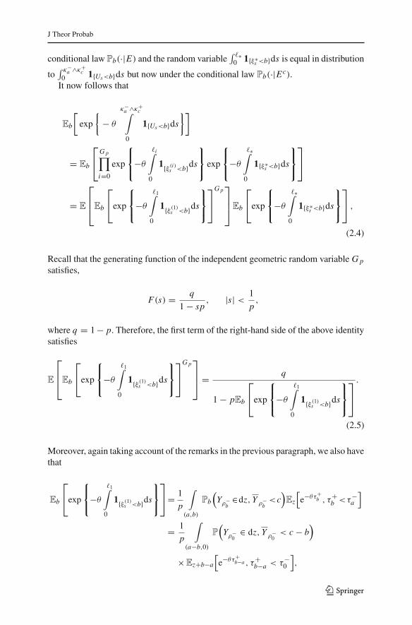
conditional law Pb(·|E) and the random variable∫ �∗

0 1{ξ∗s <b}ds is equal in distribution

to∫ κ−

a ∧κ+c

0 1{Us<b}ds but now under the conditional law Pb(·|Ec).It now follows that

Eb

[exp

{− θ

κ−a ∧κ+

c∫

0

1{Us<b}ds

}]

= Eb

⎡⎣

G p∏i=0

exp

⎧⎨⎩−θ

�i∫

0

1{ξ (i)s <b}ds

⎫⎬⎭ exp

⎧⎨⎩−θ

�∗∫

0

1{ξ∗s <b}ds

⎫⎬⎭⎤⎦

= E

⎡⎢⎣Eb

⎡⎣exp

⎧⎨⎩−θ

�1∫

0

1{ξ (1)s <b}ds

⎫⎬⎭⎤⎦

G p⎤⎥⎦Eb

⎡⎣exp

⎧⎨⎩−θ

�∗∫

0

1{ξ∗s <b}ds

⎫⎬⎭⎤⎦ ,

(2.4)

Recall that the generating function of the independent geometric random variable G p

satisfies,

F(s) = q

1 − sp, |s| < 1

p,

where q = 1 − p. Therefore, the first term of the right-hand side of the above identitysatisfies

E

⎡⎢⎣Eb

⎡⎣exp

⎧⎨⎩−θ

�1∫

0

1{ξ (1)s <b}ds

⎫⎬⎭⎤⎦

G p⎤⎥⎦ = q

1 − pEb

⎡⎣exp

⎧⎨⎩−θ

�1∫

0

1{ξ (1)s <b}ds

⎫⎬⎭⎤⎦.

(2.5)

Moreover, again taking account of the remarks in the previous paragraph, we also havethat

Eb

⎡⎣exp

⎧⎨⎩−θ

�1∫

0

1{ξ (1)s <b}ds

⎫⎬⎭⎤⎦= 1

p

∫

(a,b)

Pb

(Yρ−

b∈dz, Y ρ−

b<c

)Ez

[e−θτ+

b , τ+b <τ

−a

]

= 1

p

∫

(a−b,0)

P

(Yρ−

0∈ dz, Y ρ−

0< c − b

)

× Ez+b−a

[e−θτ+

b−a , τ+b−a < τ−

0

],

123

J Theor Probab

where Y t = sup0≤s≤t Ys . From the Compensation Formula (see for instance identity(8.27) in [10]), one can deduce

P

(Yρ−

0∈ dz, Y ρ−

0< c − b

)= W(0+)

W(c − b)

c−b∫

0

W(c − b − y)(dz − y)dy, (2.6)

and from identity (8.8) in [10], we have

Ez+b−a

[e−θτ+

b−a , τ+b−a < τ−

0

]= W (θ)(z + b − a)

W (θ)(b − a). (2.7)

Therefore, from (2.6) and (2.7), we get for each i

Eb

⎡⎣exp

⎧⎨⎩−θ

�i∫

0

1{ξ (i)s <b}ds

⎫⎬⎭⎤⎦

= W(0+)p

c−b∫

0

∫

(a−b,0)

W(c − b − y)

W(c − b)

W (θ)(z + b − a)

W (θ)(b − a)(dz − y)dy.

It is worth noting at this point that W(0+) > 0 precisely because we have restrictedourselves to the case of bounded variation paths.

The classical ruin problem for Y tells us that

P(ρ−

0 < ∞) ={

1 if ψ ′(0+)− δ ≤ 0,

1 − (ψ ′(0+)− δ)W (0+) if ψ ′(0+)− δ > 0,

see for example formula (8.7) in [10]. Taking limits as c ↑ ∞ the formula with (2.6),making use of Exercise 8.5 in [10] which tells us that limc↑∞ W(c−b−y)/W(c−b) =exp{−ϕ(0)y}, we get

1 = W(0+)(ψ ′(0+)− δ)+ + W(0+)∞∫

0

∫

(−∞,0)

(dz − y)e−ϕ(0)ydy.

Hence putting all the pieces together in (2.5), we obtain

E

[Eb

[exp

{− θ

�1∫

0

1{ξ (1)s <b}ds

}]G p]

= q

W(0+)(ψ ′(0+)− δ)+ + W(0+)∞∫

0

∫

(−∞,0)

B(θ)(z, a, b, c, y)(dz − y)dy

,

(2.8)

123

J Theor Probab

where

B(θ)(z, a, b, c, y)=e−ϕ(0)y − W(c − b − y)

W(c − b)

W (θ)(z + b − a)

W (θ)(b − a)1(a−b,0)(z)1(0,c−b)(y).

Next, we compute the Laplace transform of∫ �∗

0 1{ξ∗s <b}ds. Recalling that �∗ is equal

in law to κ−a ∧ κ+

c under Pb(·|Ec) we have two cases to consider. In the first case, theprocess Y continuously exits the interval [b, c] at c. In the second case, the processU exits the interval [b, c] downwards by a jump, if the process jumps into [a, b), itcontinues until it jumps again below a. Hence from identities (8.8), (8.9) in [10] and(2.6), we have

Eb

[exp

{− θ

�∗∫

0

1{ξ∗s <b}ds

}]

= 1

q

(Pb

(ρ+

c < ρ−b

)+∫

(a,b)

Pb

(Yρ−

b∈ dz, Y ρ−

b< c

)Ez

[e−θτ−

a , τ−a < τ+

b

])

= 1

q

(W(0+)

W(c − b)+

∫

(a−b,0)

P

(Yρ−

0∈ dz, Y ρ−

0< c − b

)Ez+b−a

[e−θτ−

0 , τ−0 < τ+

(b−a)

])

= 1

q

(W(0+)

W(c − b)+ W(0+)

c−b∫

0

∫

(a−b,0)

(Z (θ)(z + b − a)− Z (θ)(b − a)

× W (θ)(z + b − a)

W (θ)(b − a)

)W(c − b − y)

W(c − b)(dz − y)dy

). (2.9)

Let

A(θ)(z, a, b, c, y) = G(θ)(z, a, b)W(c − b − y)

W(c − b)1(a−b,0)(z)1(0,c−b)(y),

where we recall G(θ)(z, a, b) was defined in (1.7).Plugging (2.8) and (2.9) back into (2.4), we get the desired identity. �

3 Proof of Theorem 1: Unbounded Variation Paths, σ 2 = 0

In this part of the proof, we extend the previous calculations to unbounded variationLévy process with no Gaussian component (σ = 0). There is a very particular reasonwhy we do not consider the inclusion of the Gaussian component, which is related tosmoothness properties of scale functions. We shall address this issue at the end of thesection.

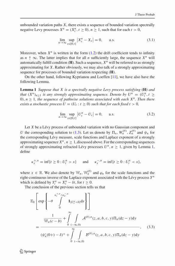
To start with we recall the following well-established result which can be founddiscussed, for example on p. 210 of [2]. For any spectrally negative Lévy process with

123

J Theor Probab

unbounded variation paths X , there exists a sequence of bounded variation spectrallynegative Levy processes Xn = (Xn

t , t ≥ 0), n ≥ 1, such that for each t > 0,

limn→∞ sup

s∈[0,t]∣∣Xn

s − Xs∣∣ = 0, a.s. (3.1)

Moreover, when Xn is written in the form (1.2) the drift coefficient tends to infinityas n ↑ ∞. The latter implies that for all n sufficiently large, the sequence Xn willautomatically fulfill condition (H). Such a sequence, Xn will be referred to as stronglyapproximating for X . Rather obviously, we may also talk of a strongly approximatingsequence for processes of bounded variation respecting (H).

On the other hand, following Kyprianou and Loeffen [11], we have also have thefollowing Lemma.

Lemma 1 Suppose that X is a spectrally negative Levy process satisfying (H) andthat (Xn)n≥1 is any strongly approximating sequence. Denote by U n = (U n

t , t ≥0), n ≥ 1, the sequence of pathwise solutions associated with each Xn. Then thereexists a stochastic process U = (Ut : t ≥ 0) such that for each fixed t > 0,

limn→∞ sup

s∈[0,t]∣∣U n

s − Us∣∣ = 0, a.s. (3.2)

Let X be a Lévy process of unbounded variation with no Gaussian component andU the corresponding solution to (1.3). Let us denote by n,W (θ)

n , Z (θ)n and ψn forthe corresponding Lévy measure, scale functions and Laplace exponent of a stronglyapproximating sequence Xn, n ≥ 1, discussed above. For the corresponding sequencesof strongly approximating refracted Lévy processes U n, n ≥ 1, given by Lemma 1,define

κ+,nx = inf{t ≥ 0 : U n

t > x} and κ−,nx = inf{t ≥ 0 : U n

t < x},

where x ∈ R. We also denote by Wn,W(θ)n and ϕn for the scale functions and the

right-continuous inverse of the Laplace exponent associated with the Lévy process Y n

which is defined by Y nt = Xn

t − δt , for t ≥ 0.The conclusion of the previous section tells us that

Eb

⎡⎢⎣exp

⎧⎪⎨⎪⎩−θ

κ+,nc ∧κ−,n

a∫

0

1{U ns <b}ds

⎫⎪⎬⎪⎭

⎤⎥⎦

=

1

Wn(c − b)+

∞∫

0

∫

(−∞,0)

A(θ),n(z, a, b, c, y)n(dz − y)dy

(ψ ′n(0+)− δ)+ +

∞∫

0

∫

(−∞,0)

B(θ),n(z, a, b, c, y)n(dz − y)dy

, (3.3)

123

J Theor Probab

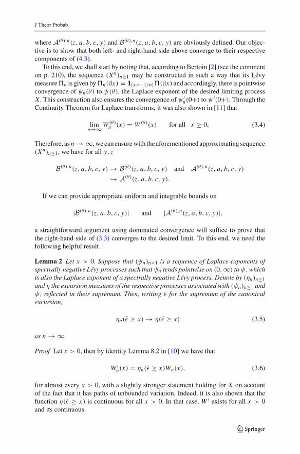
where A(θ),n(z, a, b, c, y) and B(θ),n(z, a, b, c, y) are obviously defined. Our objec-tive is to show that both left- and right-hand side above converge to their respectivecomponents of (4.3).

To this end, we shall start by noting that, according to Bertoin [2] (see the commenton p. 210), the sequence (Xn)n≥1 may be constructed in such a way that its Lévymeasuren is given byn(dx) = 1{x<−1/n}(dx) and accordingly, there is pointwiseconvergence of ψn(θ) to ψ(θ), the Laplace exponent of the desired limiting processX . This construction also ensures the convergence ofψ ′

n(0+) toψ ′(0+). Through theContinuity Theorem for Laplace transforms, it was also shown in [11] that

limn→∞ W (θ)

n (x) = W (θ)(x) for all x ≥ 0, (3.4)

Therefore, as n → ∞, we can ensure with the aforementioned approximating sequence(Xn)n≥1, we have for all y, z

B(θ),n(z, a, b, c, y) → B(θ)(z, a, b, c, y) and A(θ),n(z, a, b, c, y)

→ A(θ)(z, a, b, c, y).

If we can provide appropriate uniform and integrable bounds on

|B(θ),n(z, a, b, c, y)| and |A(θ),n(z, a, b, c, y)|,

a straightforward argument using dominated convergence will suffice to prove thatthe right-hand side of (3.3) converges to the desired limit. To this end, we need thefollowing helpful result.

Lemma 2 Let x > 0. Suppose that (ψn)n≥1 is a sequence of Laplace exponents ofspectrally negative Lévy processes such thatψn tends pointwise on (0,∞) toψ , whichis also the Laplace exponent of a spectrally negative Lévy process. Denote by (ηn)n≥1and η the excursion measures of the respective processes associated with (ψn)n≥1 andψ , reflected in their supremum. Then, writing ε for the supremum of the canonicalexcursion,

ηn(ε ≥ x) → η(ε ≥ x) (3.5)

as n → ∞.

Proof Let x > 0, then by identity Lemma 8.2 in [10] we have that

W ′n(x) = ηn(ε ≥ x)Wn(x), (3.6)

for almost every x > 0, with a slightly stronger statement holding for X on accountof the fact that it has paths of unbounded variation. Indeed, it is also shown that thefunction η(ε ≥ x) is continuous for all x > 0. In that case, W ′ exists for all x > 0and its continuous.

123

J Theor Probab

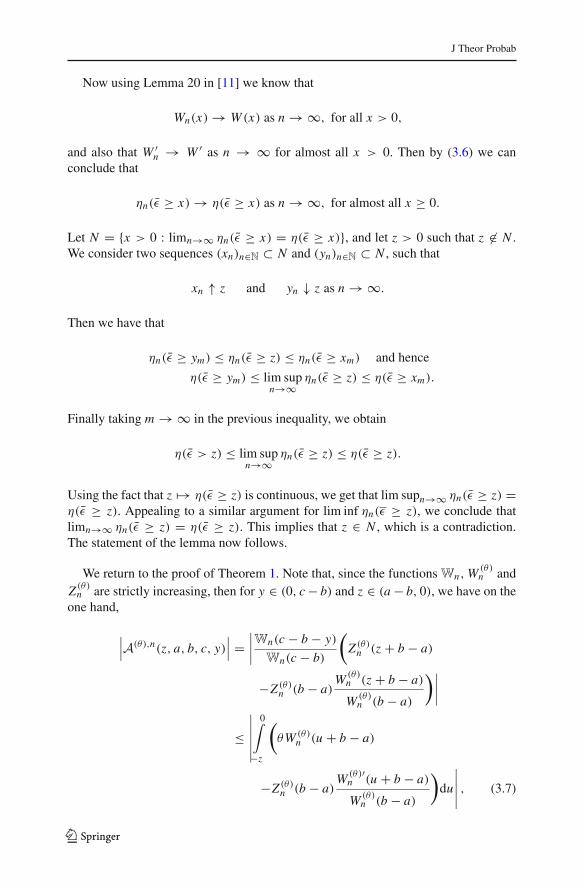
Now using Lemma 20 in [11] we know that

Wn(x) → W (x) as n → ∞, for all x > 0,

and also that W ′n → W ′ as n → ∞ for almost all x > 0. Then by (3.6) we can

conclude that

ηn(ε ≥ x) → η(ε ≥ x) as n → ∞, for almost all x ≥ 0.

Let N = {x > 0 : limn→∞ ηn(ε ≥ x) = η(ε ≥ x)}, and let z > 0 such that z �∈ N .We consider two sequences (xn)n∈N ⊂ N and (yn)n∈N ⊂ N , such that

xn ↑ z and yn ↓ z as n → ∞.

Then we have that

ηn(ε ≥ ym) ≤ ηn(ε ≥ z) ≤ ηn(ε ≥ xm) and hence

η(ε ≥ ym) ≤ lim supn→∞

ηn(ε ≥ z) ≤ η(ε ≥ xm).

Finally taking m → ∞ in the previous inequality, we obtain

η(ε > z) ≤ lim supn→∞

ηn(ε ≥ z) ≤ η(ε ≥ z).

Using the fact that z �→ η(ε ≥ z) is continuous, we get that lim supn→∞ ηn(ε ≥ z) =η(ε ≥ z). Appealing to a similar argument for lim inf ηn(ε ≥ z), we conclude thatlimn→∞ ηn(ε ≥ z) = η(ε ≥ z). This implies that z ∈ N , which is a contradiction.The statement of the lemma now follows.

We return to the proof of Theorem 1. Note that, since the functions Wn,W (θ)n and

Z (θ)n are strictly increasing, then for y ∈ (0, c − b) and z ∈ (a − b, 0), we have on theone hand,

∣∣∣A(θ),n(z, a, b, c, y)∣∣∣ =

∣∣∣∣Wn(c − b − y)

Wn(c − b)

(Z (θ)n (z + b − a)

−Z (θ)n (b − a)W (θ)

n (z + b − a)

W (θ)n (b − a)

)∣∣∣∣

≤∣∣∣∣∣∣

0∫

−z

(θW (θ)

n (u + b − a)

−Z (θ)n (b − a)W (θ)′

n (u + b − a)

W (θ)n (b − a)

)du

∣∣∣∣∣ , (3.7)

123

J Theor Probab

where we have used the monotonicity of Wn in the inequality. Next we recall, forexample from formulae (2.18) and (2.19) of [7], that

W (θ)′n (u)

W (θ)n (u)

= η�n(θ)n (ε ≥ u)+�n(θ) (3.8)

almost everywhere, where η�n(θ)n is the excursion measure of Xn under the exponential

change of measure

dP�n(θ),n

dP

∣∣∣∣∣Ft

= e�n(θ)Xnt −θ t , t ≥ 0,

with Ft = σ(Xs : s ≤ t). The right-hand side of (3.8) is a non-increasing function. Itis therefore, straightforward to check, with the help of Lemma 2 (note that the Laplaceexponent of (Xn,P�n(θ),n) is equal to ψn(· + �n(θ)) − θ and this tends pointwiseto ψ(· + �(θ)) − θ on (0,∞)) that the integrand on the right-hand side of (3.7) isuniformly bounded. Hence, there exists a constant K > 0 such that for all y, z andsufficiently large n,

∣∣∣A(θ),n(z, a, b, c, y)∣∣∣ ≤ K |z|1(a−b,0)(z)1(0,c−b)(y) (3.9)

which is integrable with respect to (dz − y)dy on (0,∞)2. Indeed, to confirm thelatter, noting that is a finite measure away from the origin, it suffices to check, withthe help of Fubini’s Theorem, that for sufficiently small ε > 0,

ε∫

0

∫

(−ε,0)(−z)(dz − y)dy =

ε∫

0

∫

(−ε−y,−y)

1(−ε,0)(z)(−y − z)(dz)dy

=∫

(−ε,0)

∞∫

0

1(0,ε)(y)1(−z−ε,−z)(y)(−y − z)dy(dz)

= −1

2

∫

(−ε,0)(z + y)2

∣∣∣−z

0(dz)

= 1

2

∫

(−ε,0)z2(dz) < ∞. (3.10)

The Dominated Convergence Theorem now implies that

limn→∞

∫

(−∞,0)

∞∫

0

A(θ),n(z, a, b, c, y)n(dz − y)dy

123

J Theor Probab

=∫

(−∞,0)

∞∫

0

A(θ)(z, a, b, c, y)(dz − y)dy.

Now let us check the integral in the denominator of (3.3). Proceeding as before, wenote that the functions Wn,W (θ)

n are strictly increasing. Then we may find an upperbound for B(θ),n(z, a, b, c, y) as follows

∣∣∣B(θ)(z, a, b, c, y)∣∣∣=

∣∣∣∣e−ϕn(0)y − Wn(c − b − y)

Wn(c − b)

W (θ)n (z + b − a)

W (θ)n (b − a)

1(a−b,0)(z)1(0,c−b)(y)

∣∣∣∣

≤ 1 + Wn(c − b − y)

Wn(c − b)

W (θ)n (z + b − a)

W (θ)n (b − a)

≤ 2. (3.11)

It follows that, provided we consider the part of the integral

∞∫

0

∫

(−∞,0)

B(θ),n(z, a, b, c, y)n(dz − y)dy (3.12)

which concerns values of y and z which are bounded away from zero, we may appealto dominated convergence to pass the limit in n through the integral in the obviousway.

Let us therefore turn our attention to the part of (3.12) which concerns small valuesof y and z. First note that we can write for ε sufficiently small,

ε∫

0

∫

(−ε,0)B(θ),n(z, a, b, c, y)n(dz − y)dy

=ε∫

0

∫

(−ε−y,−y)

B(θ),n(z + y, a, b, c, y)n(dz)dy.

In the spirit of (3.7), we can write

B(θ),n(z + y, a, b, c, y)− B(θ),n(z, a, b, c, 0) =y∫

0

∂

∂uB(θ),n(z + u, a, b, c, u)du,

where the derivative is understood as a density with respect to Lebesgue measure(on account of the fact that scale functions only have, in general, a derivative almosteverywhere). Using similar reasoning to the derivation of the inequality (3.9), we mayalso deduce that, for 0 < y, |z| < ε and ε sufficiently small,

123

J Theor Probab

∣∣∣B(θ),n(z + y, a, b, c, y)− B(θ),n(z, a, b, c, 0)∣∣∣ ≤ K1 y

for some constant K1 > 0. With similar reasoning, we can also check that, within thesame regime of y and z,

∣∣∣B(θ),n(z, a, b, c, 0)∣∣∣ ≤ K2|z|,

where K2 > 0 is a constant. We now claim that K1 y + K2|z| is a suitable dominatingfunction on 0 < y, |z| < ε. Taking account of the computations in (3.10), to verifythe last claim, it suffices to check that for ε sufficiently small,

ε∫

0

∫

(−ε−y,−y)

1(−ε,0)(z)yn(dz)dy =∫

(−ε,0)

∞∫

0

y1(0,−z)(y)dyn(dz)

= 1

2

∫

(−ε,0)z2n(dz) < ∞.

Thus far, we have shown that the right-hand side of (3.3) converges to the desiredexpression. To deal with the left hand side of (3.3), let us note that, according to theproof of Lemma VII.23 in [2], we have that P-a.s.

limn→∞ κ

+,na = κ+

a , and limn→∞ κ

−,nc = κ−

c .

Finally, using the uniform convergence of U n to U on fixed, bounded intervals of timetogether with the dominated convergence Theorem, we obtain

limn→∞ Eb

⎡⎢⎣exp

⎧⎪⎨⎪⎩−θ

κ+,na ∧κ−,n

c∫

0

1{U ns <b}ds

⎫⎪⎬⎪⎭

⎤⎥⎦ = Eb

⎡⎢⎣exp

⎧⎪⎨⎪⎩−θ

κ+a ∧κ−

c∫

0

1{Us<b}ds

⎫⎪⎬⎪⎭

⎤⎥⎦ .

Hence taking limits in both sides of (3.3) give us the desired result. ��Let us conclude this section by commenting on why we have excluded the case

σ 2 > 0. As we have seen above, we have taken account of the continuity of scalefunctions with respect to the underlying Lévy triplet in taking limits through an approx-imating sequence of processes. Had the target Lévy process X included a Gaussiancomponent, then, as we shall see in the next section, we would have found the appear-ance of derivatives of scale functions in the limit on the right-hand side of (3.3).Whilst scale functions are continuous, they do not in general have continuous deriva-tives. Indeed, for processes of bounded variation, in the case that the Lévy measure hasatoms, the associated scale functions are at best almost everywhere differentiable. Forspectrally negative Lévy processes of unbounded variation, however, scale functionsare continuously differentiable suggesting that it would be more convenient to deal thecase of σ 2 > 0 by working with an approximating sequence of unbounded variationprocesses. This is precisely what we do in the next section.

123

J Theor Probab

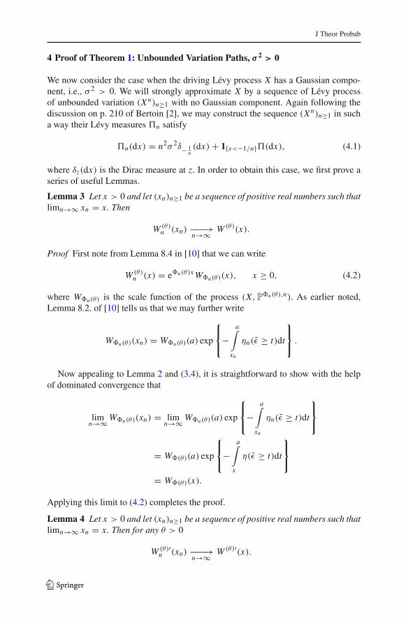
4 Proof of Theorem 1: Unbounded Variation Paths, σ 2 > 0

We now consider the case when the driving Lévy process X has a Gaussian compo-nent, i.e., σ 2 > 0. We will strongly approximate X by a sequence of Lévy processof unbounded variation (Xn)n≥1 with no Gaussian component. Again following thediscussion on p. 210 of Bertoin [2], we may construct the sequence (Xn)n≥1 in sucha way their Lévy measures n satisfy

n(dx) = n2σ 2δ− 1n(dx)+ 1{x<−1/n}(dx), (4.1)

where δz(dx) is the Dirac measure at z. In order to obtain this case, we first prove aseries of useful Lemmas.

Lemma 3 Let x > 0 and let (xn)n≥1 be a sequence of positive real numbers such thatlimn→∞ xn = x. Then

W (θ)n (xn) −−−→

n→∞ W (θ)(x).

Proof First note from Lemma 8.4 in [10] that we can write

W (θ)n (x) = e�n(θ)x W�n(θ)(x), x ≥ 0, (4.2)

where W�n(θ) is the scale function of the process (X,P�n(θ),n). As earlier noted,Lemma 8.2. of [10] tells us that we may further write

W�n(θ)(xn) = W�n(θ)(a) exp

⎧⎨⎩−

a∫

xn

ηn(ε ≥ t)dt

⎫⎬⎭ .

Now appealing to Lemma 2 and (3.4), it is straightforward to show with the helpof dominated convergence that

limn→∞ W�n(θ)(xn) = lim

n→∞ W�n(θ)(a) exp

⎧⎨⎩−

a∫

xn

ηn(ε ≥ t)dt

⎫⎬⎭

= W�(θ)(a) exp

⎧⎨⎩−

a∫

x

η(ε ≥ t)dt

⎫⎬⎭

= W�(θ)(x).

Applying this limit to (4.2) completes the proof.

Lemma 4 Let x > 0 and let (xn)n≥1 be a sequence of positive real numbers such thatlimn→∞ xn = x. Then for any θ > 0

W (θ)′n (xn) −−−→

n→∞ W (θ)′(x).

123

J Theor Probab

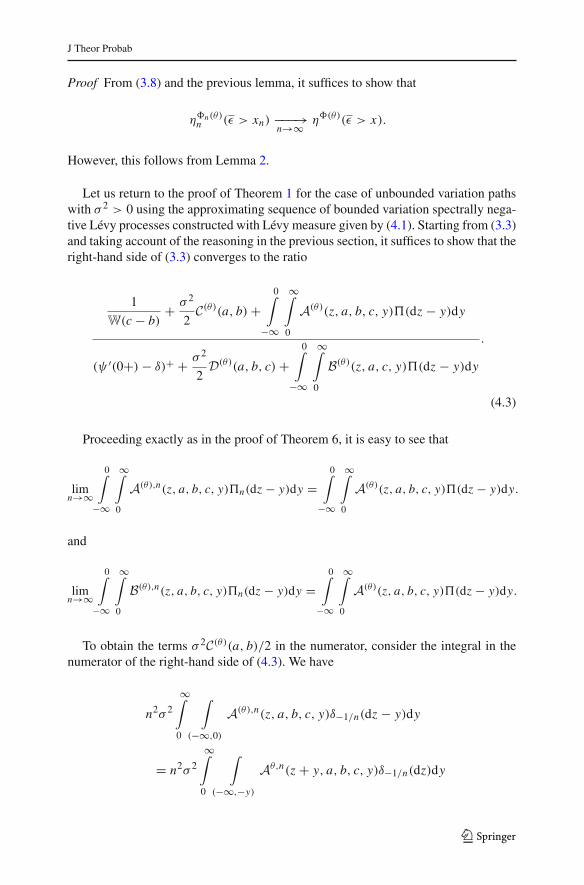
Proof From (3.8) and the previous lemma, it suffices to show that

η�n(θ)n (ε > xn) −−−→

n→∞ η�(θ)(ε > x).

However, this follows from Lemma 2.

Let us return to the proof of Theorem 1 for the case of unbounded variation pathswith σ 2 > 0 using the approximating sequence of bounded variation spectrally nega-tive Lévy processes constructed with Lévy measure given by (4.1). Starting from (3.3)and taking account of the reasoning in the previous section, it suffices to show that theright-hand side of (3.3) converges to the ratio

1

W(c − b)+ σ 2

2C(θ)(a, b)+

0∫

−∞

∞∫

0

A(θ)(z, a, b, c, y)(dz − y)dy

(ψ ′(0+)− δ)+ + σ 2

2D(θ)(a, b, c)+

0∫

−∞

∞∫

0

B(θ)(z, a, c, y)(dz − y)dy

.

(4.3)

Proceeding exactly as in the proof of Theorem 6, it is easy to see that

limn→∞

0∫

−∞

∞∫

0

A(θ),n(z, a, b, c, y)n(dz − y)dy =0∫

−∞

∞∫

0

A(θ)(z, a, b, c, y)(dz − y)dy.

and

limn→∞

0∫

−∞

∞∫

0

B(θ),n(z, a, b, c, y)n(dz − y)dy =0∫

−∞

∞∫

0

A(θ)(z, a, b, c, y)(dz − y)dy.

To obtain the terms σ 2C(θ)(a, b)/2 in the numerator, consider the integral in thenumerator of the right-hand side of (4.3). We have

n2σ 2

∞∫

0

∫

(−∞,0)

A(θ),n(z, a, b, c, y)δ−1/n(dz − y)dy

= n2σ 2

∞∫

0

∫

(−∞,−y)

Aθ,n(z + y, a, b, c, y)δ−1/n(dz)dy

123

J Theor Probab

= n2σ 2

1/n∫

0

Wn(c − b − y)

Wn(c − b)

(Z (θ)n (y − 1/n + b − a)

−Z (θ)n (b − a)W (θ)

n (y − 1/n + b − a)

W (θ)n (b − a)

)dy.

It follows that

n2σ 2

∞∫

0

∫

(−∞,0)

A(θ),n(z, a, b, c, y)δ−1/n(dz − y)dy

= n2σ 2

1/n∫

0

Wn(c − b − y)

Wn(c − b)

(Z (θ)n (y − 1/n + b − a)

−Z (θ)n (b − a)W (θ)

n (y − 1/n + b − a)

W (θ)n (b − a)

)dy

= n2σ 2

1/n∫

0

yW

′n(c − b − y)

Wn(c − b)

(Z (θ)n (y − 1/n + b − a)

−Z (θ)n (b − a)W (θ)

n (y − 1/n + b − a)

W (θ)n (b − a)

)dy

−n2σ 2

1/n∫

0

yWn(c − b − y)

Wn(c − b)

(θW (θ)

n (y − 1/n + b − a)

−Z (θ)n (b − a)W (θ)′

n (y − 1/n + b − a)

W (θ)n (b − a)

)dy

= σ 2

1∫

0

uW

′n(c − b − u/n)

Wn(c − b)

(Z (θ)n ((u − 1)/n + b − a)

−Z (θ)n (b − a)W (θ)

n ((u − 1)/n + b − a)

W (θ)n (b − a)

)du

−σ 2

1∫

0

yWn(c − b − u/n)

Wn(c − b)

(θW (θ)

n ((u − 1)/n + b − a)

−Z (θ)n (b − a)W (θ)′

n ((u − 1)/n + b − a)

W (θ)n (b − a)

)du,

123

J Theor Probab

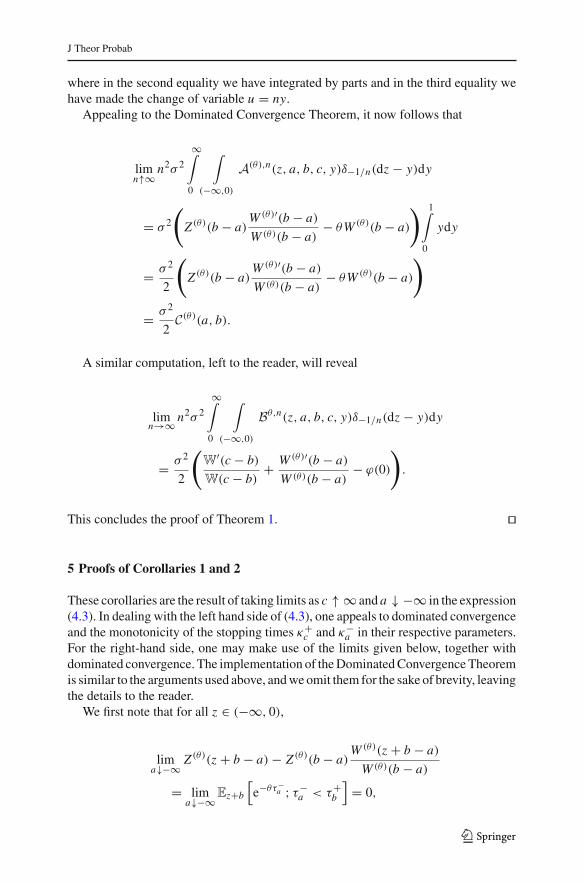
where in the second equality we have integrated by parts and in the third equality wehave made the change of variable u = ny.

Appealing to the Dominated Convergence Theorem, it now follows that

limn↑∞ n2σ 2

∞∫

0

∫

(−∞,0)

A(θ),n(z, a, b, c, y)δ−1/n(dz − y)dy

= σ 2

(Z (θ)(b − a)

W (θ)′(b − a)

W (θ)(b − a)− θW (θ)(b − a)

) 1∫

0

ydy

= σ 2

2

(Z (θ)(b − a)

W (θ)′(b − a)

W (θ)(b − a)− θW (θ)(b − a)

)

= σ 2

2C(θ)(a, b).

A similar computation, left to the reader, will reveal

limn→∞ n2σ 2

∞∫

0

∫

(−∞,0)

Bθ,n(z, a, b, c, y)δ−1/n(dz − y)dy

= σ 2

2

(W

′(c − b)

W(c − b)+ W (θ)′(b − a)

W (θ)(b − a)− ϕ(0)

).

This concludes the proof of Theorem 1. ��

5 Proofs of Corollaries 1 and 2

These corollaries are the result of taking limits as c ↑ ∞ and a ↓ −∞ in the expression(4.3). In dealing with the left hand side of (4.3), one appeals to dominated convergenceand the monotonicity of the stopping times κ+

c and κ−a in their respective parameters.

For the right-hand side, one may make use of the limits given below, together withdominated convergence. The implementation of the Dominated Convergence Theoremis similar to the arguments used above, and we omit them for the sake of brevity, leavingthe details to the reader.

We first note that for all z ∈ (−∞, 0),

lima↓−∞ Z (θ)(z + b − a)− Z (θ)(b − a)

W (θ)(z + b − a)

W (θ)(b − a)

= lima↓−∞ Ez+b

[e−θτ−

a ; τ−a < τ+

b

]= 0,

123

J Theor Probab

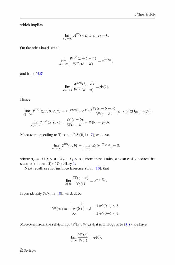
which implies

lima↓−∞ A(θ)(z, a, b, c, y) = 0.

On the other hand, recall

lima↓−∞

W (θ)(z + b − a)

W (θ)(b − a)= e�(θ)z,

and from (3.8)

lima↓−∞

W (θ)′(b − a)

W (θ)(b − a)= �(θ).

Hence

lima↓−∞ B(θ)(z, a, b, c, y) = e−ϕ(0)y − e�(θ)z

W(c − b − y)

W(c − b)1(a−b,0)(z)1(0,c−b)(y).

lima↓−∞ D(θ)(a, b, c) = W

′(c − b)

W(c − b)+�(θ)− ϕ(0).

Moreover, appealing to Theorem 2.8 (ii) in [7], we have

lima↓−∞ C(θ)(a, b) = lim

a↓−∞ E0(e−θσb−a ) = 0,

where σa = inf{t > 0 : Xt − Xt > a}. From these limits, we can easily deduce thestatement in part (i) of Corollary 1.

Next recall, see for instance Exercise 8.5 in [10], that

limz↑∞

W(z − x)

W(z)= e−ϕ(0)x .

From identity (8.7) in [10], we deduce

W(∞) =⎧⎨⎩

1

ψ ′(0+)− δif ψ ′(0+) > δ,

∞ if ψ ′(0+) ≤ δ.

Moreover, from the relation for W′(z)/W(z) that is analogous to (3.8), we have

limz↑∞

W′(z)

W(z)= ϕ(0).

123

J Theor Probab

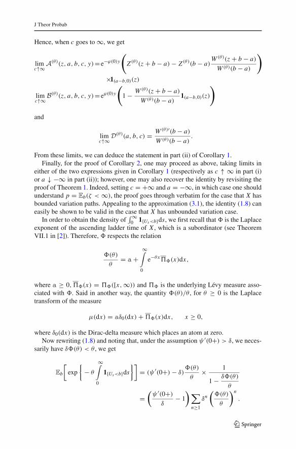
Hence, when c goes to ∞, we get

limc↑∞ A(θ)(z, a, b, c, y)= e−ϕ(0)y

(Z (θ)(z + b − a)− Z (θ)(b − a)

W (θ)(z + b − a)

W (θ)(b − a)

)

×1(a−b,0)(z)

limc↑∞ B(θ)(z, a, b, c, y)= eϕ(0)y

(1 − W (θ)(z + b − a)

W (θ)(b − a)1(a−b,0)(z)

)

and

limc↑∞ D(θ)(a, b, c) = W (θ)′(b − a)

W (θ)(b − a).

From these limits, we can deduce the statement in part (ii) of Corollary 1.Finally, for the proof of Corollary 2, one may proceed as above, taking limits in

either of the two expressions given in Corollary 1 (respectively as c ↑ ∞ in part (i)or a ↓ −∞ in part (ii)); however, one may also recover the identity by revisiting theproof of Theorem 1. Indeed, setting c = +∞ and a = −∞, in which case one shouldunderstand p = Eb(ζ < ∞), the proof goes through verbatim for the case that X hasbounded variation paths. Appealing to the approximation (3.1), the identity (1.8) caneasily be shown to be valid in the case that X has unbounded variation case.

In order to obtain the density of∫∞

0 1{Us<b}ds, we first recall that� is the Laplaceexponent of the ascending ladder time of X , which is a subordinator (see TheoremVII.1 in [2]). Therefore, � respects the relation

�(θ)

θ= a+

∞∫

0

e−θx�(x)dx,

where a ≥ 0,�(x) = �([x,∞)) and � is the underlying Lévy measure asso-ciated with �. Said in another way, the quantity �(θ)/θ , for θ ≥ 0 is the Laplacetransform of the measure

μ(dx) = aδ0(dx)+�(x)dx, x ≥ 0,

where δ0(dx) is the Dirac-delta measure which places an atom at zero.Now rewriting (1.8) and noting that, under the assumption ψ ′(0+) > δ, we neces-

sarily have δ�(θ) < θ , we get

Eb

[exp

{− θ

∞∫

0

1{Us<b}ds

}]= (ψ ′(0+)− δ)

�(θ)

θ× 1

1 − δ�(θ)

θ

=(ψ ′(0+)δ

− 1

)∑n≥1

δn(�(θ)

θ

)n

.

123

J Theor Probab

We deduce that∫∞

0 1{Us<b}ds has a density which is given by

(ψ ′(0+)δ

− 1

)∑n≥1

δnμ∗n(dx), x ≥ 0,

where μ∗n is the n-fold convolution of μ. Note that μ∗n({0}) = an and hence, withν(dx) = �(x)dx , we finally come to rest at

Pb

⎛⎝

∞∫

0

1{Us<b}d ∈ dx

⎞⎠=

(ψ ′(0+)δ

−1

)⎛⎝ δa

1 − δaδ0(dx)+1{x>0}

∑n≥1

δnν∗n(dx)

⎞⎠ ,

where ν∗n is the n-fold convolution of ν. ��Acknowledgments J.-L. P. acknowledges financial support from CONACyT Grant no. 129326. J.-C.P. acknowledges financial support from CONACyT Grant no. 128896. A. E. K. acknowledges financialsupport from the Santander Research Fund.

References

1. Avram, F., Palmowski, Z., Pistorius, M.R.: On the optimal dividend problem for a spectrally negativeLévy process. Ann. Appl. Probab. 17, 156–180 (2007)

2. Bertoin, J.: Lévy Processes. Cambridge University Press, Cambridge (1996)3. Chow, Y.S., Teicher, H.: Independence Interchangeability Martingales. Springer, New Yok (1978)4. Furrer, H.: Risk processes perturbed by α-stable Lévy motion. Scand. Actuar. J. 1998(1), 59–74 (1998)5. Huzak, M., Perman, M., Šikic, H., Vondracek, Z.: Ruin probabilities and decompositions for general

perturbed risk processes. Ann. Appl. Probab. 14, 1378–1397 (2004)6. Huzak, M., Perman, M., Šikic, H., Vondracek, Z.: Ruin probabilities for competing claim processes.

J. Appl. Probab. 41, 679–690 (2004)7. Kuznetsov, A., Kyprianou, A.E., Rivero, V.: The theory of scale functions for spectrally negative Lévy

processes. Lévy Matters II, Springer Lecture Notes in Mathematics (2013)8. Klüppelberg, C., Kyprianou, A.E., Maller, R.A.: Ruin probabilities and overshoots for general Lévy

insurance risk processes. Ann. Appl. Probab. 14, 1766–1801 (2004)9. Klüppelberg, C., Kyprianou, A.E.: On extreme ruinous behaviour of Lévy insurance risk processes. J.

Appl. Probab. 43(2), 594–598 (2006)10. Kyprianou, A.E.: Introductory Lectures on Fluctuations of Lévy Processes with Applications. Springer,

Berlin (2006)11. Kyprianou, A.E., Loeffen, R.: Refracted Lévy processes. Ann. Inst. H. Poincaré 46(1), 24–44 (2010)12. Kyprianou, A.E., Palmowski, Z.: Distributional study of de Finetti’s dividend problem for a general

Lévy insurance risk process. J. Appl. Probab. 44, 349–365 (2007)13. Landriault, D., Renaud, J-F., Zhou, X.: Insurance risk models with Parisian implementation delays,

Submitted (2011) www.ssrn.com/abstract=174419314. Landriault, D., Renaud, J.-F., Zhou, X.: Occupation times of spectrally negative Lévy processes with

applications. Stoch. Process. Appl. 121, 2629–2641 (2011)15. Lambert, A., Simatos, F., Zwart, B.: Scaling limits via excursion theory: interplay between Crump-

Mode-Jagers branching processes and processor-sharing queues. To appear in Ann. Appl. Prob. (2013)16. Loeffen, R. L., Renaud, J-F., Zhou, X.: Occupation times of intervals untill first passage times for

spectrally negative Lévy processes with applications. Submitted (2012) arxiv:1207.159217. Renaud, J.-F., Zhou, X.: Distribution of the dividend payments in a general Lévy risk model. J. Appl.

Probab. 44, 420–427 (2007)18. Song, R., Vondracek, Z.: On suprema of Lévy processes and application in risk theory. Ann. lnst. H.

Poincaré 44, 977–986 (2008)

123