Obtaining Order in a World of Chaos - IEEE Signal ...

easurements of a physical or biological system result in a t ime series, s ( t ) = ~ ( t , + nz, ) = ~ ( n ) , sampled at intervals of z, and initiated at to,. When a

signal can be represented as a superposition of sine waves with hfferent amplitudes, its characteristics can be adequately described by Fourier coefficients of amplitude and phase. In these circumstances, linear and Fourier- based methods for extracting information from the signal are appropriate and powerful. However, the signal may be generated by a nonlinear system. The waveform can be irregular and continuous and broadband in the frequency domain. The signal is noise-like, but is deterministic and may be chaotic. More information than the Fourier coefficients is required to describe the signal [l, 21. This article describes methods for distinguishing chaotic signals from noise, and how to utilize the properties of a chaotic signal for classification, prediction, and control.

A measured signal that has an irregular time series and a continuous, broadband power spectrum is dstin- guishable from noise and can occur within the dynamics of a few degree- of-freedom dynamical system. To describe such a signal with the infinite number of Fourier coefficients is not appropriate. One goal of this article is to describe a class of practical techniques for dealing with such signals. These techniques enable one to easily:

Determine directly from measured data how many degrees of freedom are operating to produce the signal,

Determine the predictability of the underlying dynamics from these observations,

Although these methods were developed primarily from studies of chaotic systems, they also are useful for characterizing and exploiting all types of signals.

Data from a nonlinear circuit [3] (Fig. 1 ) will be used to illustrate the general points of the article. The differential equations for this circuit are:

~- dy(t) - - X ( t ) - @(t) + z ( t ) d t

= y[af(x(t)) - z ( t ) ] -oy(t) dt

where x ( t ) and z ( t ) are the voltages across the capacitors, Make simple, useful predictive models, Identify parameters in a system of (nonlinear)

equations devised to describe the original source of

C and C’; c1 is the gain of the nodinear converter atx = 0; and y ( t ) = J(t)( L / C)’”. Time (t) has been normalized with respect to (LC)-’’’. The nonlinear response of the converter, N, is approximated well by the piecewise nonlinear function Devise control strategies for nonlinear processes.

MAY 1998 IEEE SIGNAL PROCESSING MAGAZINE 1053-5888/98/$10.000 1998IEEE

49

0.528 if x 5 -12 x ( l - x 2 ) if -12<x<12

‘l’he other parameters ofthe model are dependent on the linear feedback loop through

(3)

For circuit elements withR = 3.98 ld2 ,~ ‘ = 361R, C = 23.01 aF, C’ = 334 aF, L = 152.6 mtl, and a = 24.24, the output is the time series of Fig. 2 where the sampling rate is 50 liHz (T$ = 0.02ms).

This is an example of a signal arising from the deterministic dynamics of a three-degree-of-freedom system. The power spectrum (Fig. 3) is broad and continuous and the autocorrelation function (Fig. 4) rapidly goes to zero. Using methods that will be described in detail in the next section, the dynamical structure of this signal can be cap- tured using a three-dimensional state space created from the measured voltage x(a) = x(t , + nzz I ) and its time lags, T. Using a time lag of 15 samples (T = 1 5 ~ ~ = 0.3ms) three-dimensional vectors are created:

to produce the three-dimensional object displayed in Fig. 5(a).

This article describes how to transform the measurements, ~ ( n ) , to the geometric object associated with the source of the signal and how to extract dynamical information from that object. Knowledge of the dynamical system or the governing dfferential equations is not required to analyze the signal. A more detailed explanation of the underlying theory and methods is in reference [4]. The software used for this analysis is called “csp” (cspW for Windows, cspX for UNIX) [ 51.

The state of a dynamical system at any time can be specified by a state-space vector where the coordmates of the vector are the independent degrees of freedom of the system. For the circuit of Fig. 1, the state of the system is given by y (n ) = [x (n ) , y(n), z(n)] a t any time, n = t o + nz, . Generally, the number of first-order differential equations describing the system determines the number of independent components in y(n). The “embedding theorem” [ 1,2,6] establishes that, when there is only a single measured quantity from a dynamical system, it is possible to reconstruct a state space that is equivalent to the original (but unknown) state space composed of all the dynamical variables.

The embedding theorem [7-91 states that if the system produces orbits in the original state space that lie

50 IEEE SIGNAL PROCESSING MAGAZINE MAY 1998

on a geometric object of dimensiond, (which need not be integer), then the object can be unambiguously seen without any spurious intersections of the orbit in another space of integer dimension d > 2d,, or larger, comprised of coordinates that are (almost) arbitrary nonlinear transformations of original state-space coordinates. The absence of intersections in the second space means the orbit is resolved without ambiguity when d is large enough. Overlaps of the orbit may occur in lower dimensions and the ambiguity at the intersections destroys the possibility of predicting the evolution of the system.

In a dissipative system, the geometric object to which orbits go in time is callcd the system attractor. If d, is not integer, it is called a strange attractor (after Ruelle [lo]), and the system is chaotic. It is the attractor and the motion of system orbits on it, not the projection of those motions onto the observation axis of the measurements, where prediction, classification, control, and other signal-processing tasks can be carried out without ambiguity. That is, it is necessary to go to a higher- dimensional space to do signal processing when the signal comes from a nonlinear system that may exhibit irregular, chaotic motions.

Almost any set of d coordinates is equivalent by the embedding theorem. Each set is a different way ofunfold- ing the attractor from its projection onto the observations. Formally, an autonomous system producing orbits x(6) through the dynamics is

-- dx(t) - F(x(t)), dt

and the output is s ( t ) = h(x( t ) ) . x is an n-dimensional vector, and s ( t ) is typically a onedmensional output signal. With mild restrictions on the functions F(x) and h(x), any independent set of quantities related to s ( t ) can serve as the coordinates for a state space for the system. Time derivatives of s ( t ) are the natural set of independent coordinates. But, when the signal is sampled in discrete time, the derivatives are a high-pass filter and therefore emphasize errors and noise in the measurements. The first derivative of s ( t ) is approximated by

s ( t , + (n + l)T, ) - S(t, + nzz, ) i(n) =

7, (6)

which is also a high-pass filter. Equation 6 suggests another natural set of coordmates

for the state space. The signal s(n) and its time delays are the ingredients in the approximations to the time derivatives of s(n). The time-delay values of s(n) are new information that enters the approximation of each derivative. Using the observed signal and its time delays avoids the emphasis on errors and noise associated with high-pass filter approximations to the time derivatives and requires no computation on the observations themselves. This set of coordinates is realized by forming the vectors

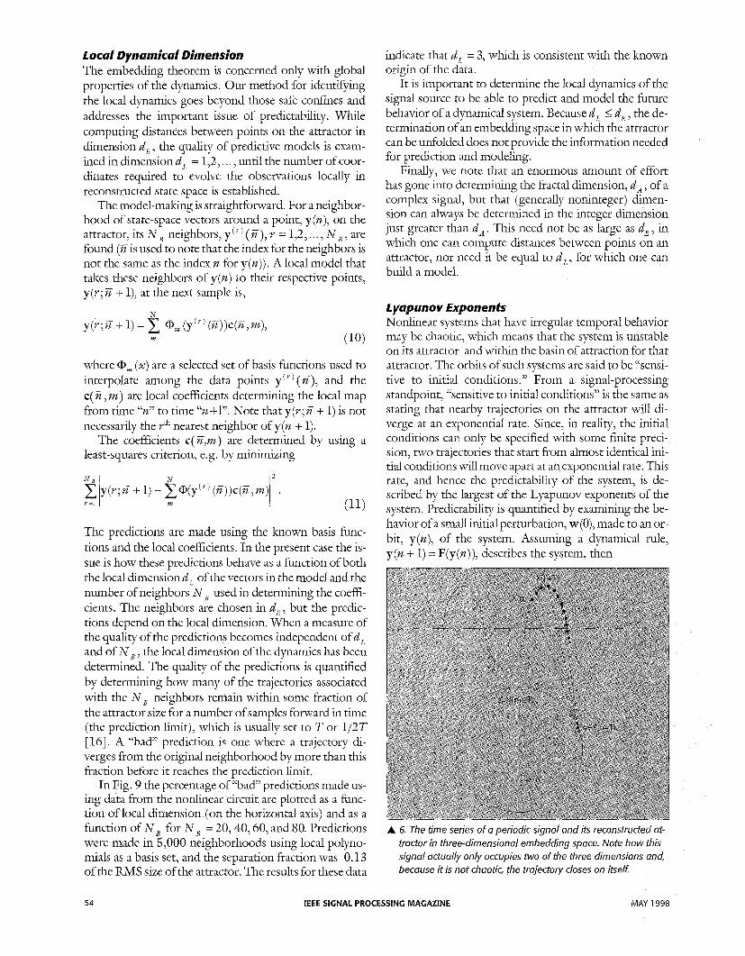
where a dE dimensional state space is constructed, and each component of the vector y(n) is separated in time by TT , (T is an integer, as is d, ) . An example of this reconstruction for a simple periodic signal is shown in Fig. 6. In this case, the attractor is a closed loop that can be embedded in a two-dimensional space (although three are used for the display-this signal is over embedded). To do this embedding, a time delay, T, and the number of components, d, , in the vector y (n) are needed.

Choosing a Time Delay When the signal is represented by Eq. (7), assurance is needed that each component of the vector is providing new information about the signal source at a given time. The dynamical difference between the components is achieved by the evolution of the signal source for a time Tz, .This time must be large enough so that all dynamical degrees-of-freedom coupled to the variable s ( t ) have the opportunity to influence the value of s ( t ) . Yet, Tmust also be small enough so that the inherent instabilities of nonlinear systems do not contaminate the measurement at a later time, Tz I . The embedding theorem provides assurance that, were there an infinite amount of infinitely accurate data, any T would work, and these concerns would vanish. But, since there is usually only a finite amount of

A 1. The circuit diagram of a nonlinear and chaotic circuit.

finite precision data, these are practical concerns of a seri- ous nature.

The fundamental issue is that there must be a balance between values of T that are too small (where each component of the vector does not add significant new information about the dynamics), and values of T that are too large. Large values of T create uncorrelated elements in y(n) because of the instabilities in the nonlinear system that become manifest over time. Thus, the components of y (n ) will become independent and convey no knowledge of the system dynamics.

A correlation function between the measurements s(n) and s(n + T ) is needed to describe their nonlinear depend- ence on each other. Because of the way the signal source conveys information to the observer, a natural correlation fhction is Shannon’s mutual information [ 113. If there are two sets of measurements, a l , a 2 ,..., a, and b, , 6, , ,,, bK, then the amount of information (in bits) about measurement a that is acquired by observing b, is

A 2. The time series of output voltage from the circuit of Fig. 1. The sampling rate is 50 kHz (T$ = 0.02 ms).

MAY 1998 IEEE SIGNAL PROCESSING MAGAZINE 51

where PA (a) is the probability of measurement a, P, (b) is the probability of measurement b, and P, (a, b) is the joint probability ofmeasurements a andb. For these computations, the measurements a are the s(n), and the b, are the s(n + T). These are deterministic signals, so the probability is the distribution of values of the variables as a function of time. PA (a) is the normalized histogram ofthe aj observations andP, (b) is the normalized histogram for the 6,. The joint histogram is P, (a, b).

Thus, the suitable nonlinear correlation function is the mutual information of the measurements, averaged over all measurements

I

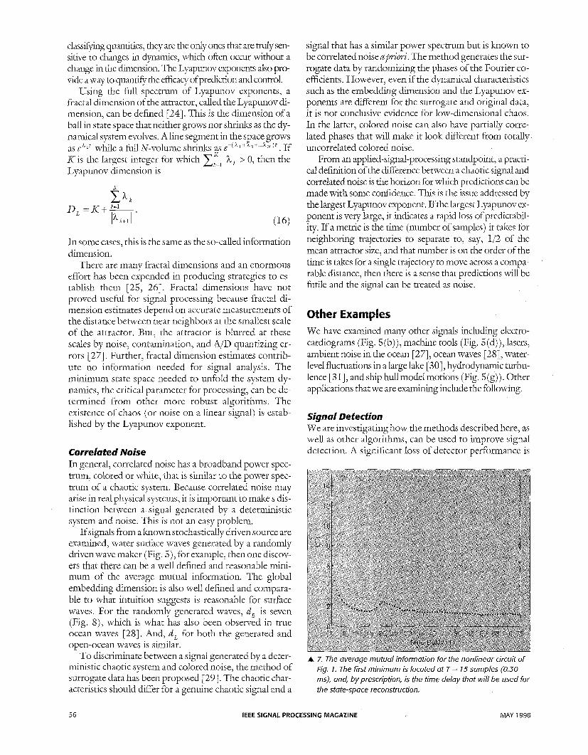
I ( T ) 2 0 for all T, so there is not a zero value analogous to the familiar linear correlation function, which is some- times advocated for selecting the time delay. An alternative prescription for nonlinear correlation is to use the value of T at the first minimum of I (T ) to create the vectors y(n) [ 12,131. For the circuit data, the average mutual information evaluated using 215 samples is shown in Fig. 7 where the first minimum is at T = 15.

The choice of the first minimum of I (T) is aprescw$J- tion, not a rigorous fmed choice. In general, the prescription provided by the average mutual information often appears to yield a shorter time delay than the first zero crossing of the autocorrelation function. The danger in using the longer time delay is that the components of the vector can become independent of each other and subsequent calculations may not be valid (this can happen with the Lyapunov exponents, for example). Thus, an even safer procedure is to evaluate the important dynamical quantities, such as the Lyapunov exponents, over a range of time delays.

~ m ~ i ~ n The embedding theorem [7, 81 provides a sufficient dimension in which the orbits of the system are no longer crossing each other and the temporal sequence of points is without ambiguity. The data may not require this large a dimension, and by following the general sense of the embedding theorem there is another way to choose the number of coordinates [ 141. For any point on the attractor, y(n) , one can ask whether its nearest neighbor in a state space of lmension d is there for dynamical reasons or is instead projected into the neighborhood because the dimension is too small. That neighbor is then examined in dimension d + 1 by simply adding another coordinate to y (n ) using the time-delay construction. If the nearest neighbor is a true neighbor, meaning it arrived there

A 3. The Fourier power spectrum for 65,536 samples of the nonlinear circuit.

A 4. The autocorrelation function for the nonlinear circuit, as a function of the time lag.

dynamically, it will remain a neighbor in this larger space. If that nearest neighbor is there because dimension d is too small, it will move away from y(n) as dimensions are added. When the number of these false nearest neighbors becomes zero, the attractor has been unambiguously unfolded because crossings of the orbit have been eliminated. The dimension in which false neighbors disappear is the dimension necessary for viewing the data. This minimum embedding dimension, d, , is less than or equal to the sufficient dimension found from the embedding theorem.

Desirable neighbors lie close by virtue of the evolving dynamics of the system. In practice, however, there are four types of neighbors, only one of which are true neighbors:

TyGe ne&hbws that result from the dynamics of the system. These neighbors are acceptable and can be used for analysis, prediction, and control.

False nearest ne&hbom result from a projection of the attractor into an insufficient dimension, as discussed above.


Ovevsampby ne@bors arise from using too high a sampling rate. This causes the next point on the orbit to always be identified as the nearest neighbor and misses the recur- rent visits to the neighborhood of the point in question.

Qwntized neighbors that arise from rounlng error, for example, from an A/D converter.

False nearest neighbors are the result of using too low an embedding dimension. An ambiguity results where the trajectory crosses itself. At such a crossing, one cannot tell which path the trajectory should follow, in the absence of other information. The consequences for prediction algorithms and analysis methods that rely on the behavior of close neighbors can be disastrous. Form- nately, false neighbors are easy to detect and are eliminated by selecting an appropriate embedding dimension.

Oversampled neighbors result from a high sampling rate or may arise when a low-pass filter has been applied to data. Subsequent samples may be so close in time that they are closer than neighbors that are more distant in time, but are also close in state space (the true neighbors). Oversampled neighbors are easily eliminated. When searching for neighbors, one simply requires that they have some reasonable temporal separation. Because the sample number is a proxy for time, it is easy to require that candidate neighbors be separated by a reasonable number of samples, usually the time delay.

The final type of neighbor poses a severe problem that is not easily resolved. Because AID converters use a finite number of bits, a rounding error occurs. This may happen when a converter with a small number of bits is used, or if the range of signal activity is small relative to the range expected by the converter. Suppose there are two floating-point numbers, known to six significant digits, suchas 128.123456and 128.123123. If, inthecollection or conversion process, these are rounded to 128.123 they become the same number. When this happens, then there is a probability that low-dimensional vectors formed from the numbers will also have this ambiguity. Vectors that are actually distinct in state space all collapse to a single vector. There is no ideal way to fur this, although the effects can be mitigated.

It is easy to sort the points in dimension d by how close they are to y(n) [ 151. We use Euclidean distance, but any distance measure will work. Once sorted, it is straightforward to examine the nearest neighbor of every point, and thus identify any false neighbors in the selected dimension. As the dimension is increased from d = 1 to d = 2, . . . , the percentage of false nearest neighbors should go to zero at the dimension where the attractor is globally unfolded [ 141. This is the minimum global embedding dimension, d,. A residual of false nearest neighbors is caused by contamination of the data by a high- dimensional signal that is conveniently called “noise.” Noisy data have nonzero false neighbors because the attractor is blurred. As d increases, the noise component slowly begins to predominate. Thus, there is a strong mo- tivation not to over embed noisy signals.

Figure 8 is the percentage of false nearest neighbors out of 65,536 samples from the nonlinear circuit. The data vectors for the nonlinear circuit are constructed in dimension d = 1,2, .. .10 using the time delay of T = 15 chosen from the prescription by average mutual information. It is clear that the false nearest neighbors disappear at d, = 3. Once there are no false nearest neighbors left, further unfolding of the attractor has no effect. These data are relatively noise free, so no rise in false nearest neighbors is seen as d increases beyondd, . However, the correlated noise and the EKG data show the residual that is characteristic of noise.

Local Properties of the Dynamics The dynamics associated with the circuit develop locally on the attractor through some discrete-time map or through differential equations. The number of degrees- of-freedom, d,, governing the dynamics is less than, or equal, to the global embedding dimension d, . dE can be greater than d L , because the coordinate system is created solely from measured data. This coordinate system may twist and fold the attractor relative to its geometry in the original, but unknown, coordinates of the dynamical system. However, if the dynamical system has only d, degrees-of-freedom locally, that information can be used to classify the dynamics and construct a framework for predictive models and control strategies. For example, the attractor corresponding to periodic motion is a closed loop in the state space (local dimension d, = 1) although generically it may oiily be unfolded in three-dimensional space (d, = 3).

A 5. Reconstructed attractors for a variefy of systems.


amical Dimension The embedding theorem is concerned only with global properties of the dynamics. Our method for identifying the local dynamics goes beyond those safe confines and addresses the important issue of predictability. While computing distances between points on the attractor in dimension d, , the quality of predctive models is examined in dimension d, = 1,2,. . . , until the number of coordinates required to evolve the observations locally in reconstructed state space is established.

The model-making is straightforward. For a neighborhood of state-space vectors around a point, y(n), on the attractor, its N , neighbors, y‘” ( E ) , r = 1,2, ... , N , , are found (%is used to note that the index for the neighbors is not the same as the index n for y(n)). A local model that takes these neighbors of y (n ) to their respective points, y(v;% + l), at the next sample is,

where (x) are a selected set of basis functions used to interpolate among the data points y(+‘j(%), and the c( %, m ) are local coefficients determining the local map from time %” to time %+I”. Note that y(+;E + 1) is not necessarily the v* nearest neighbor of y(n + 1).

The coefficients c(E,m) are determined by using a least-squares criterion, e.g. by minimizing

N y(v;% + 1) - - p ( y ‘ Y ) (E) )c (E ,m)

m

The predictions are made using the known basis functions and the local coefficients. In the present case the issue is how these predictions behave as a function of both the local dimension d, of the vectors in the model and the number of neighbors N , used in determining the coefficients. The neighbors are chosen in d,, but the predictions depend on the local dimension. When a measure of the quality of the predictions becomes independent of d, and of N , , the local dmension of the dynamics has been determined. The quality of the predictions is quantified by determining how many of the trajectories associated with the N , neighbors remain within some fraction of the attractor size for a number of samples forward in time (the prediction limit), which is usually set to T o r 1/2T [16]. A “bad” prediction is one where a trajectory di- verges from the original neighborhood by more than this fraction before it reaches the prediction limit.

In Fig. 9 the percentage of “bad” predictions made using data from the nonlinear circuit are plotted as a function of local dimension (on the horizontal axis) and as a function of N , for N , = 20,40,60, and 80. Predictions were made in 5,000 neighborhoods using local polynomials as a basis set, and the separation fraction was 0.13 of the RMS size of the attractor. The results for these data

indcate that d, = 3, which is consistent with the known origin of the data.

It is important to determine the local dynamics of the signal source to be able to predct and model the future behavior of a dynamical system. Because d, 5 d, , the de- termination of an embedding space in which the attractor can be unfolded does not provide the information needed for prediction and modeling.

Finally, we note that an enormous amount of effort has gone into determining the fractal dimension, d, , of a complex signal, but that (generally noninteger) dimension can always be determined in the integer dimension just greater than d, . This need not be as large as dE , in which one can compute distances between points on an attractor, nor need it be equal to d,, for which one can build a model.

Lyapuno v Exponents Nodnear systems that have irregular temporal behavior may be chaotic, which means that the system is unstable on its attractor and within the basin of attraction for that attractor. The orbits of such systems are said to be “sensitive to initial conditions.’’ From a signal-processing standpoint, “sensitive to initial conditions’’ is the same as stating that nearby trajectories on the attractor will di- verge at an exponential rate. Since, in reality, the initial conditions can only be specified with some finite precision, two trajectories that start from almost identical initial condtions wdl move apart at an exponential rate. This rate, and hence the predictability of the system, is described by the largest of the Lyapunov exponents of the system. Predctability is quantified by examining the behavior of a small initial perturbation, w(O), made to an orbit, y(n), of the system. Assuming a dynamical rule, y(n + 1) = F(y(n)), describes the system, then

A 6. The time series of a periodic signal and its reconstructed attractor in three-dimensional embedding space. Note how this signal actually only occupies two of the three dimensions and, because it is not chaotic, the trajectory closes on itself.

54 lEEE SIGNAL PROCESSINC MAGAZINE MAY 1998

or in the limit as w(n) + 0

~ ( n + 1) = DF(y(n)). W(W)

= DF(y(n)). DF(y(n - 1))**. DF(y(O))w(O) = DF’ ( ~ ( 0 ) ) . ~ ( 0 ) . (13)

The Jacobian matrix of the dynamics is

DF(x), = - aF, (XI ; a,b= 1 2 , ... d. (14)

where DF (x) is the composition of n Jacobians calcu- lated at iterations of a starting point, x.

The stability of the system for the small perturbation w(0) is determined by the eigenvalues of the matrix DF (y(n)) after L samples along the orbit after the perturbation. Oseledec [ 171 analyzed this eigenvalue problem, which is a generalization of the familiar linear stability problem for perturbations about a fEed point or equilibrium orbit. The matrix

is well defined because the product of DFL and its transpose is orthogonal. As L becomes large (in a formal sense, as L -+ 00 ) the eigenvalues of th s matrix have been shown to exist for almost all x along an orbit and are independent of x. The eigenvalues are also unchanged under a smooth nonlinear transformation of the coordinate system, which means that the dynamical system can be classified with these eigenvalues. Regardless of the coordinate system, the computed values will be the same. The eigenvalues are e h , , e h , , . . . , eh , in a d-dimensional system where by convention h , 2 h 2.. . h , are the global Lyapunov exponents [18].

If any of the h are positive, then the oryt is unstable. Dissipation in the dynamics requires h a < 0, so that volumes in state space shrink as time p;o!&esses. This leads to the manifestation of the instability on the attractor, although it remains a compact geometric object in the state space. If any of the h It are greater than zero, the system is chaotic by definition. If one of the ha is zero, then the dynamical system producing the signal can be described by a set of ordinary differential equations. It is possible for a discrete time dynamical system to have a zero Lyapunov exponent, but the parameter values for the system would be exceptional.

are evaluated by numerically determining the DF(x) locally in state space from the local predictive maps described above. The linear term in these maps gives DF(x). The composition of the Jacobians can be di- agonalized by a recursive decomposition method, even though the product is ill conditioned. The values of the

The h

Lyapunov exponents, L, samples forward (or backward) in time after a perturbation at x can be determined from OSL(L,x). These are the local Lyapunov exponents, h , (L,x) [19-211, and their average over many initial conditions, x, are denoted ha (L).

The ha (L) converge to the global exponents, h a , as a power ofL. It is useful to display the h a (t) as a finction of L to identify the zero exponent, if it exists, as well as characterize the general trend of all exponents. Fig. 10 shows the average local Lyapunov exponents for the example circuit that were evaluated from knowledge of the scalar measurement, x(t), alone. The near zero global exponent indicates that a set of three ordinary differential equations is required for the description of the data.

This method directly evaluates the d, exponents. If a dimension of d, were used for the computations, there would be d, - d, false Lyapunov exponents with little sense of which were the true exponents and which were false. In principle, the extraneous exponents should be negative and represent the orbit moving from some point in state space onto the attractor. In practice, this rarely happens. One can either select d,, using the local false nearest neighbor algorithm or, if there is enough noise- free data, evaluate the h, (L) forward and backward, which produces d, exponents that change sign and d, - d, exponents that do not change sign. The correct d, exponents are the ones that change sign [22,23].

If the sum of the exponents is greater than zero, the results are meaningless. This can occur when the signal mi- grates through state space instead of remaining in a bounded region (a situation typical of much financial data), if the signal is nonstationary, or if the trajectories are not coherent for some reasonable period of time. The latter may result when the underlying system is stochastic. In this case, close trajectories may even go in opposite dlrections.

The sum of the Lyapunov exponents may also be greater than zero if too large a time delay is selected, in which case the observations that make up the vector y(n) have become independent. Thus, an examination of the sum of the exponents is necessary to ensure the interpre- tation of the largest exponent is valid. For example, one prescription for selecting the time delay is to use the first zero-crossing of the autocorrelation function. For the ex- emplar nonlinear circuit, Fig. 4 leads to a choice of T = 100. But, if this time delay is used to compute the Lyapu- nov exponents, the sum of the exponents is positive and the largest exponent, despite the fact it is invalid, is almost 20 times larger than the value that results from using T = 15. The implication for prediction is that the if the larger time delay were accepted, the horizon to which one could predict would be greatly reduced (or nonexistent). The prescription provided by Fraser [ 12,131 does not always generate the smallest value of h , (which provides the greatest predlctability), but in our experience, it never overestimates the time delay.

The Lyapunov exponents are perhaps the most important quantifying measure of chaotic motions. Of all the


classlfsiing quantities, they are the only ones that are truly sensitive to changes in dynamics, whch often occuy without a change in the dunension. The Lyapunov exponents also provide a way to quantfy the efficacy of prediction and control.

Using the full spectrum of Lyapunov exponents, a fractal dimension of the attractor, called the Lyapunov dimension, can be defined [24]. This is the dimension of a ball in state space that neither grows nor shrinks as the dynamical system evolves. Aline segment in the space grows

. If IC is the largest integer for which h =1 h > 0, then the Lyapunov dmension is

as ehlt while a &UN-volume shrinks ;s

In some cases, this is the same as the so-called information dimension.

There are many fractal dimensions and an enormous effort has been expended in producing strategies to es- tablish them [25, 261. Fractal dimensions have not proved useful for signal processing because fractal dimension estimates depend on accurate measurements of the distance between near neighbors at the smallest scale of the attractor. But, the attractor is blurred at these scales by noise, contamination, and AID quantizing errors [27]. Further, fractal dimension estimates contrib- ute no information needed for signal analysis. The minimum state space needed to unfold the system dynamics, the critical parameter for processing, can be determined from other more robust algorithms. The existence of chaos (or noise on a linear signal) is established by the Lyapunov exponent.

Correlated Noise In general, correlated noise has a broadband power spectrum, colored or white, that is similar to the power spectrum of a chaotic system. Because correlated noise may arise in real physical systems, it is important to make s dis- tinction between a signal generated by a deterministic system and noise. This is not an easy problem.

Ifsignals from a luiown stochastically driven source are examined, water surface waves generated by a randomly driven wave inalcer (Fig. 5), for example, then one discov- ers that there can be a well defined and reasonable minimum of the average mutual information. The global embedding dimension is also well defined and compara- ble to what intuition suggests is reasonable for surface waves. For the randomly generated waves, d, is seven (Fig. 8), which is what has also been observed in true ocean waves [28]. And, d, for both the generated and open-ocean waves is similar.

To discriminate between a signal generated by a deterministic chaotic system and colored noise, the method of surrogate data has been proposed [29]. The chaotic characteristics should differ for a genuine chaotic signal and a

signal that has a similar power spectrum but is lmown to be correlated noise apvi0.u.i. The method generates the surrogate data by randomizing the phases of the Fourier coefficients. However, even if the dynamical characteristics such as the embedding dimension and the Lyapunov exponents are lfferent for the surrogate and original data, it is not conclusive evidence for low-dmensional chaos. In the latter, colored noise can also have partially correlated phases that will make it loolc lffereiit from totally uncorrelated colored noise.

From an applied-signal-processing standpoint, a practical defintion of the difference between a chaotic signal and correlated noise is the horizon for whch predctions can be made with some confidence. This is the issue addressed by the largest Lyapunov exponent. If the largest Lyapunov exponent is very large, it inlcates a rapid loss of prelctabil- ity. If a metric is the time (number of samples) it t a l a for neighboring trajectories to separate to, say, 112 of the mean attractor size, and that number is on the order of the time is takes for a single trajectory to move across a compa- rable distance, then there is a sense that prelctions will be & d e and the signal can be treated as noise.

We have examined many other signals including electrocardiograms (Fig. 5(b)), machine tools (Fig. 5(d)), lasers, ambient noise in the ocean [27], ocean waves [28], water- level fluctuations in a large lake [ 301, hydrodynamic turbulence [ 3 11, and shp hull model motions (Fig. 5 (g) ) . Other applications that we are examining include the following.

Signal Defection We are investigating how the methods described here, as well as other algorithms, can be used to improve signal detection. A significant loss of detector performance is

A 7. The average mutual information for the nonlinear circuit of Fig. 1. The first minimum is located at T = 15 samples (0.30 ms), and, by prescription, is the time delay that will be used for the state-space reconstruction.


typically due to the mismatch between the noise statistics assumed in a matched filter and the true statistics of environ- mental noise and clutter. Depending on the context, the loss may be on the order of 10 dJ3 or more. A better understand- ing of the true nature of noise can be used to improve signal-detector performance by mitigating the mismatch between the assumed and the true noise. Prototypes of methods to do this have been constructed and have demon- strated significant gains over existing processors.

Electrocardiograms (EKGs) The electrophysiology of the heart is complex because it involves interactions among multiple physiological variables including autonomic and central nervous regula- tion, hemodynamic and humoral effects, and other extrinsic variables. Yet, the instrumentation for measurements are often limited to electrocardiograms from skin- mounted sensors. This is precisely the type of situation where the tools described in this article are most powerful. The system is a multivariate nonlinear system, yet it is possible to collect only one type of signal.

An additional difficulty arises from the nature of the collection. The period over which the system is stationary is short (literally, how long will a human subject remain motionless while data are collected?), the sensors are not calibrated, and there is a great deal of variability among subjects. A further complication is the dearth of data, es- pecially from healthy subjects. People without health problems rarely undergo extensive cardiac testing where high-quality data can be collected.

Nonetheless, there are some consistent results. The strange attractor of an EKG is shown in Fig. S(b). It is typical of resting-state EKGs and, along with other cases, has a global embedding dimension of five and a local dynamical dimension of four. In fact, for the cases we have examined, the d, is almost always five and the d, is almost always four. Our experiments to date include subjects who are undergoing a stress test for a specific pathology and these dimension measures vary little during the test. For almost all cases, including one extreme pathology, dimension measures remain relatively con- stant. The one nonlinear characterization of the data that does change, as a preliminary finding, is the spectrum of Lyapunov exponents.

The extreme pathology is ventricular fibrillation. The dimensions still appear to be d, = 5 and d, = 4, but the largest Lyapunov exponent is different from the other cases. In fact, given considerations of the short periods over which such data can be collected and instrumentation calibration and noise, it appears that a distinguishing hallmark of this life-threatening condition is that the largest Lyapunov exponent can be considered to be near zero-the system is not chaotic. Thus, while the statistical base is still small, there is evidence that laowledge about the diversity of chaos is beneficial and that it has practical applications in classifying cardiac behavior.

Radar Backscatter In a companion article in this issue, Simon Haykin reviews some of his research on radar backscattering from the ocean surface. The IPIX X-band radar was land mounted 25 to 30 meters above sea level, which is a typical height for a ship-mounted radar. The antenna was fEed, so that the system operated in a dwell mode and il- luminated a fixed patch of the ocean surface. The tempo-

~


A 8. False nearest neighbors as a function of the dimension of the reconstructed state space vectors [x(n), x(n + g, . . ., x(n + (d- 1)q. The global embedding dimension, where the percentage of false nearest neighbors goes to zero, is d, = 3 for the nonlinear circuit. The low number of false nearest neighbors for the neurons in d, = 1 is caused by quantizing errors. Note also how the minimum for the correlated noise has a large residual, then increases, which is typical of how noise fills the state space as the embedding dimension increases.

A 9. Local false nearest neighbors for the nonlinear circuit. The percentage of " b a d projections is plotted as a function of the model dimension (horizontal axis) and the number of neighbors used in making the local predictive model. N, = 20, 40, 60 and 80. The quality of prediction becomes independent of model dimension and N, at d, = 3.

A 10. Average local Lyapunov exponents as a function of the number of samples, L, after a perturbation. As L --f -, the global Lyapunov exponents are reached. This calculation used 65,536 reconstructed state-space vectors in d, = d,= 3. The calculation was started over 4,500 different locations on the attractor and the results were then averaged. One exponent is positive, indicating that the system is chaotic, and one exponent is zero, indicating that the dynamics are described by differential equations. One exponent is negative and large enough so that h,+h,+h, < 0.0, which means that the attractor is bounded and the calculations are bounded. The Lyapunov dimension, D , associated with this attractor is D, = 2.04.

ral data recorded was due entirely to the motion of the ocean surface. Haylun’s article addresses what appears to be the natural connection between the dimensionality of a chaotic signal and the configuration of neural networks used to extract that signal from its background. This research [32] has shown that backscatter from a low- grazing-angle radar is from a low-dimensional system where the embeddmg dimension is five (Fig. 8) and the largest Lyapunov exponent is about 0.14 (Fig. 11).

Ocean Water Levels Classification and predction of ocean water levels is important because of the need for accurate short-term water-depth predictions in shallow navigable channels. Optimum siting of tide stations is also a long-standing problem. It is desirable to minimize the number of stations in a region, but a complete description and record of the tides along all sections of the coast is imperative. An analysis of data from seven east coast U.S. tides stations shows that, in general, stations exposed to the open ocean record observations that have an observed embedding dimension of five and a local dynamical dimension of four or five [33]. However, there are large variations in the Lyapunov exponents and, for example, the largest Lyapu- nov exponent for Charleston, South Carolina, whose attractor is shown in Fig. 5, is about 0.62 while at Ft. Pulaslu, Georgia, it is about 0.78. This demonstrates how behaviors can vary within a fixed dimensionality. Inter-

estingly, for stations inside a complex estuary (Chesa- peake Bay), the embedding dimension increased to six and the Lyapunov exponents are much larger (3.91 at Baltimore, Maryland). This follows intuition in that more variables ought to be active inside the estuary and that behavior ought to be more complex. Fort Pulaslu and Charleston will be examined in the next section as an example of how one sensor’s measurements can be used to predict the behavior of a signal from another.

Characterizing nonlinear systems by the state-space analysis of observed data provides a framework for per- forming important tasks. These include malung predctions based on an observed set of data from the past [ 341, predicting one “hard” dynamical variable from the observation of an ‘‘easy‘? variable using past simultaneous measurement of both variables [ 351, and controlling dynamical systems to some more regular, or possibly to an even more irregular orbit [36]. We briefly dscuss each of these and mention other applications of the framework established by the nonlinear analysis described above. These methods have also been used to devise secure communications systems [ 371, but these applications will not be covered in this article.

prediction Using a single, scalar measurement from a nonlinear dynamical system, one can reconstruct its attractor from the methods described earlier. If the source of the signal is stationary, then the attractor remains the same whenever the observations begin, even though the actual orbit is “sensitive to initial conditions” and is uncorrelated with any past measurements. One can use the statistically stationary properties of the attractor to provide an accurate “black box” means for predicting future evolution of an orbit when the past has been well sampled. It is a “black box” procedure because no knowledge of the underlying physics of the source is required. While it provides accurate predictive power, there is a limit on the depth to which one can take this approach because of the inherent loss of predictability in a chaotic system.

The method for nonlinear estimation is similar to linear autoregressive (AR) and ICalman filter techniques except that estimation is done in the spatial and temporal domain of the attractor, rather than the frequency or traditional time domain of the signal. As with AR and I(alman fiters, an explicit model of the system is not required.

If every neighborhood of the attractor has been well visited, then the evolution of points from one state-space neighborhood to the next neighborhood can be mapped. Knowledge of a local numerical map that moves the trajectories from neighborhood to neighborhood provides a way to place any newly observed point, y(nj, into the neighborhood nearest to it and then project the trajectory


forward from that neighborhood to predict y(n + 1). The process is then repeated to move y(n + 1) to y(n + 2), and so on. The power of the method is limited by the growth of errors, as dictated by the largest Lyapunov exponent h 1, which in time = 1 / h destroys the possibility of further prediction. This is actually a limit on any method of nonupdated prediction, including direct use of the equations of motion.

To build local maps that describe the evolution of neighborhoods, we start with an observed point, y(n), on the attractor. In a neighborhood with N , neighbors y"' (E) with E = 1,2,. .. , N , , the (unknown) vector field, F(y), that evolves points on the at t ractor y(n + 1) = F(y(n)) can be expanded as

in terms o f M basis functions, cp, (y). Radial basis functions, sigmoidal functions associated with neural networks, and polynomials are widely used choices for the 'pm (y) [34]. The mathematical problem being addressed is that of interpolation within neighborhoods of a multidimensional space populated by observed data points. There are arguments for choosing any of these alterna- tives, and there are also certainly other choices with excel- lent justification.

An expansion that involves both the choice of basis function cp , ( 0 ) and M is

where y(7;E + 1) is the point to which the neighbor y"' (%) goes in one sample period (7, ). The coefficients, c(m), are chosen by a least-squares method that minimizes the error in this model of the dynamics. So minimizing

gives the coefficients c k (yn), m = 1,2, .. . , M associated with the local map, F(x), at time n. This is a standard linear problem. One of the advantages of this technique is that the coefficients can be computed as needed, so the computation burden is low.

For each new data point, z, its evolution can be predicted by first locating the nearest point in the baseline data (which provides the coefficients c (m)). Call it y o ) . Then the point that follows z is zl:

m=l

and the point z2 that follows z1 is determined by the neighborhood in which z1 falls. If the nearest point to z1 in the baseline set is y(P), then

The number of points z -+ z1 -+ z2 + ... that can be predicted accurately is limited by the largest global Lyapu- nov exponent h .

Figures 12 to 15 show predictions for the example circuit with time horizons from five to 40 samples (0.10 ms to 0.80 ms). These predictions are produced using 20,000 samples as a baseline set. In each case the samples from 30,000 to 31,600 samples are given as initial conditions and predictions are made 5, 12,25, and 40 samples ahead. The predictions are compared with the

A 1 1. Average local Lyapunov exponents for the radar backscatter data discussed in the companion article by Simon Haykin.

A 12. Predictions of the future behavior of the voltage from past observations of the voltage in the nonlinear circuit. 20,000 samples were used to make local polynomial maps on the attractor in d, = d, = 3. This figure shows predictions five samples ( 5 ~ ~ - 0.10 ms) ahead of samples 30,000 to 3 1,600, compares it with the observed values, and shows the error at each sample.


measured value at each sample. The prediction, observed values, and errors in prediction are plotted in each figure. As expected, the errors grow as the predlction horizon is extended from five samples to 40, and whle there are re- gions where the errors are small, even for predlcting 40 samples ahead, the overall degradation of predictability is apparent. A quantitative estimate of the growth of errors in this kind of prediction strategy is given in [ 381.

There is a notable similarity of these nonlinear methods and some linear methods. Global linear methods derive model coefficients from training data to use as a map that moves z (n) to z(n+l), based on some number of prior observations, such as autoregression [39]

where the coefficients bi are computed from the autocorrelation coefficients of the training data using the Yule- Wallier equations :

where cp, (i) are the autocorrelation coeffi evaluation of these terms using p prior observations or estimates is straightforward.

State-space estimation derives coefficients from previously observed data for a map that moves the vector y(n) to y ( n + 1) (note the similarity between Eqs. (20) and (22)). “Disembedding” by talung the first component of the vector y (n + 1) yields the estimate of x(n + 1).

The restrictions on linear methods require that there must be significant Fourier coefficients to compute the 6,. This is true regardless of the specific technique: AR (autoregression), ARMA (AR moving average), or Kal- man filter. The assumptions behind linear estimation hold that the signals are composed of sinusoids and superposition can be applied. If there are no significant features in the Fourier domain, then linear methods cannot work. If the signal is chaotic, then the residual yb

grows to the magnitude of the observed signal within a few samples. A primary advantage of estimation in state space is that points on the orbit that are distant in time may be close in the state space, hence lcnowledge of longer period dynamics is incorporated into the predictions. Thus, the estimator may have a lower residual, yk, over longer prediction periods.

P r @ ~ i ~ t i n ~ One Time Series From Another (Uirtual Sensor) One of the remarkable implications of the embedding theorem is that any measured variable can be used to pro-

A 13. Predictions of future behavior of the voltage x(t) from past observations of the voltage, 20,000 samples of the voltage were used to make local polynomial maps on the attractor in d, = d , = 3. This figure shows prediction 12 samples (122, - 0.24 ms) ahead of samples 30,000 to 31,600, compares it with the observed values, and shows the error at each sample.

duce coordinates for a state space that fully captures the dynamics of the signal source. This means that for two measured variables, VA(t) = VA(to + nzIA) = VA(n) and VB(t) = VB(to + nzJBj = VB(n), either one or a mixture of the two can be used to produce a state space for the dynamics. If variableA is used to create data vectors in dimension dE , then

Y A (n) = [VA (a), VA (n - TA),VA (a -2T,), ... , VA (W - (4 - 1P-A )I (24)

If d, is large enough, then no further coordinates are required. The embedding theorem requires that any other aspect of the dynamical system, such as the measurement VB(n), is determined by these vectors via

The scalar function f, ( 0 ) is not linown in general, but may be determined by expanding f ( y ( n ) ) in some con- venient basis set

Neighborhoods of simultaneous observations may also be used-the baseline data again-to determine the coefficients c, locally in state space. This means that from a set of simultaneous observations of the dynamical variables “A” and “B,” “A” can be predicted from “B” or vice-versa, which can eliminate the need to malie both measurements in the future [ 351.

There are two obvious applications for this method. One situation is the case where one of the measurements


is difficult and expensive, while the other measurement is easy and inexpensive. In such a case, simultaneous measurements of both variables would be made for some baseline period. Subsequently, the easy measurement can be used to predict the hard one. As long as the signal source is stationary, the local maps determined from the simultaneous measurements eliminate the need for the expensive observations. Alternatively, cross-predictions can be used to monitor the reliable operation of various sensors. A real-world case is power generation plants where both plant operating conditions and the sensor systems must be monitored and rapid assessment of anomalous sensor readmgs must be made. Traditionally, the monitoring of instrument performance is done using redundant moni- tors and comparison to analytical estimates of the process. In most practical cases, however, analytical knowledge of the system behavior is unavailable.

The methods of nonlinear system identification described in this article are intended for autonomous dynamical systems. With some modifications, they can also be applied to so-called input-output systems [40]. These systems do not reside on a low-dimensional attractor as they are driven by external (possibly high-dimensional) forces. Still, the internal nonlinear structure of the system can be unfolded using time-delayed reconstruction of the state vector based on scalar measurements from one or more meters.

As a demonstration of this method for plant and instrument monitoring, we analyzed multiple channel data from a pressurized water reactor power plant that was recorded for 8 hours on 28 January 1997 at a 2 second sampling interval. Two measurements, steam flow and pressurizer water level, were chosen for the cross- predictions. Using the pressurizer data, the time delay for embedding was determined to be 50 samples (100 s) based on the average mutual information, and the embedding dimension was determined to be dE = 4. Fig. 16 shows the measured steam flow, the measured pressurizer level, and the predictions of the flow that were computed from the pressurizer level measurements. Thus, the unre- liable measurement of flow rate can be monitored (or re- placed) by a nonlinear predictor based on simultaneous measurements of the reliable pressurizer water level. This type of assessment is critical for complex systems where it is essential to rapidly discriminate between true systems anomalies and sensor systems failures.

A second application of the method is to identify measur- ing sensors that are “redmdanP in the sense that the information gathered from one is accurate enough to allow the information gathered by the second to be deduced. An interesting, nontrivial, example of this situation is the poten- tial redundancy of tide stations that measure ocean and estuary water levels. The problem of water-level characterization and prediction in coastal and shallow waters is very difficult because there are many nonhear forces and mecha- nisms that act in addtion to the seemingly regular “tides.” Local meteorology and bathymetry often have an influence that exceeds the magnitude of the tidal constituents.

Because of the expense of operating tide stations, there is considerable interest in finding methods that can reduce the number of active tide stations, while improving the safety of marine navigation. Numerical models that solve the hydrodynamic equations of motion (the inherently nonlinear Navier-Stoles equations) have not been approved for op- erational use for shallow coastal waters because of the precision required for navigation, the large number of forces, the complex bathymetry, the large number of sensors that are needed, the small grid size that is required, and the computation expense. Further, predictive numerical models of water levels are dependent on other models for predictions of forces such as the local wind fields.

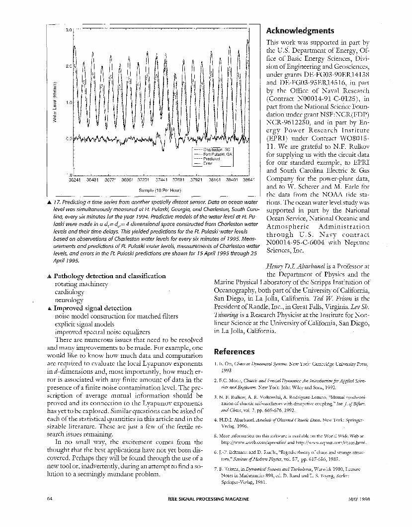
Ocean water level data at tide stations exposed to the open ocean, when analyzed by the methods in this article, have d, = 5 and d, = 4 or 5. Across surprisingly large distances, the present measurements of one station can be re- placed by a reconstructed state space made from measurements of a baseline period at another station and the function of Eqs. 25 and 26 (obviously, data must also be collected at the first station during the baseline period). Fig. 17 is the predicted water levels at the tide station at Ft. Pulaski, Georgia, based on observations at the tide station located at Charleston, South Carolina.

Simultaneous measurements of the water levels at both stations were made every six minutes throughout 1994 [41] for a total of 87,600 samples. Predictions of water levels at Ft. Pulaski were made starting at 00:06 on 1 January 1995 and continued throughout 1995. Fig. 17 displays the predictions and actual measurements for Ft. Pulaski from 04:06 on 15 April 1995 through 04:06 on 25 April 1995 along with the observations at Charleston and the prediction errors. During the period shown, the range of water-level variations at Ft.

A 14. Predictions of future behavior of the voltage x(t) from past observations of the voltage. 20,000 samples of the voltage were used to make local polynomial maps on the attractor in d,= d, = 3. This figure shows prediction 25 samples (252, - 0.50 ms) ahead of points 30,000 to 3 1,600, compares it with the observed values, and shows the error made at each sample.


A 15. Predictions of future behavior of the voltage x(f, from past observations of the voltage. 20,000 samples of the voltage were used to make local polynomial maps on the attractor in d, = d, = 3. This figure shows prediction 40 samples (407, - 0.80 ms) ahead ofpoints 30,000 to 31,600, compares it with the observed values, and shows the error made at each step.

Pulaslu was 2.16 meters, while at Charleston it was 1.63 meters. In predicting Ft. Pulaski from Charleston, we used a four-dmension space (d, for Charleston) and a first-order local linear polynomial predictor. The variance in the prediction error was 0.0029 m2 for all of 1995, which is a substantial improvement over a good statistical correlation method that yielded a variance of 0.0050 m2. In another case, water levels at Key West, Florida, were predicted from Charleston, some 940 kilometers distant, with an average error of 11%, compared to 25% for the statistical correlation [42].

Control of Chaotic Motions Chaos has little appeal to engineers seeking regular, predictable environments in which to accomplish various tasks. However, the desire to push further into interesting parameter regimes to accomplish a task faster or more thoroughly (such as optimum mixing) may stress the dynamical system in a way that results in instabilities associated with chaotic motions of the system. To transform this unwanted chaotic motion into motion that is more regular and predictable, one might try to use small variations in system parameters to control the chaotic motion. Indeed, if one could, using small forces, move the chaotic system into a part of state space where the stable parts of the dynamical motions would dominate, then the exponential contractions associated with these stable directions would produce regular orbits.

There is evidence, but no theorems, that within the motions of a system moving along a strange attractor there are, in principle, an infinite number of periodc orbits, each ofwhich is unstable in the uncontrolled, chaotic system. Each ofthese unstable periodic orbits is a solution to the equations of motion of the system and it should be

MAY 1998 62 IEEE SIGNAL PROCESSING MAGAZINE

possible, using small forces, to drive the chaotic system to a selected periodic orbit and stabilize it by a judcious choice of forces. Because any individual chaotic trajectory comes close to each of these unstable periodic orbits [ 3 ] , the required forces should be small.

The first proposal to address this problem came from Ott, Grebogi, and Yorlte (OGY) who suggested a method to drive chaotic motions to the stable directions associated with unstable periodic orbits [43]. That is, their method moves poles lying outside the unit circle all the way to the origin in eigenvalue space [44]. An alternative, less demanding view based on optimal control theory seeks to drive the poles back into the unit circle. Both work with small forces, and each is briefly described.

The OGY method is most easily described by consider- ing the observations made in discrete time intervals (coin- ciding with the period of the goal orbit) that can be unfolded in a space of dimension two. In this space, the dynamical variable is a two-dimensional vector y(n) , and the target is a fEed point Y, (a) satisfying

y p (U = 0) = F(yF (W = 0), w = 0),

where the U are parameters of the system. We presume that the a can be controlled with external forces that remain small (U =. 0 always). The dynamics are described by

A rule is needed for a(%) that places the point y(n + 1) - y, on the stable direction of the local Jacobian DF(y,). This is assured by the following control requirement [43], which is correct when a(%) = 0.

where f, is the left eigenvector of DF(y , ) associated with the unstable eigenvalue h ~ that lies outside the unit circle.

describes how the system varies with the control forces. There is a substantial amount of experimental verification of this basic OGY formula [45], yet there are several problematic aspects of the overall strategy. First, the formula requires the orbit to be in the neighborhood of the fuied point yF before control is applied. This can tale some time, but there is a clever way to work around the problem using a method called targeting [46]. Unfortu- nately, targeting requires detailed knowledge of the global stable and unstable manifold structure of the dynamics, which is difficult to acquire. The second problem with the OGY strategy is that it is difficult to apply in higher dimensions, although there are ways to work around this, and they seem to perform adequately [47]. The final problem with the method is that it requires a lot

of knowledge about the dynamical system. The eigenvec- tors and eigenvalues of the local Jacobian matrix DF(y, ) are needed in addition to g. However, all of these quantities can be evaluated in state space reconstructed from a single variable and its time delays.

An alternative to the strong requirement of the OGY method to place the unstable eigenvalues of the Jacobian matrix at the origin is to make sure they lie within the unit circle. This guarantees stabilization and requires much less detailed knowledge of the local dynamics. If this can be accomplished by an optimum control method, then there is no longer the requirement to be near the targeted unstable periodic orbit or to push unstable eigenvalues to the origin. Only knowledge of the approximate local dynamics and the variation of the vector field with respect to the control forces is required. This enables control over chaotic instabilities and allows rapid forcing of the chaotic orbits to a selected unstable periodic orbit [48].

There are at least two advantages of the dynamical systems approach to control of nonlinear systems. First, the fact that control can be done in the reconstructed state space means that detailed, accurate original state-space models of the dynamics are not required because these models can be learned well enough from observations of evolution on the attractor. Second, control of unstable periodic orbits of the chaotic system can be achieved with small control forces. The presence of these unstable peri- o d ~ orbits is new to the discussion of control. We have not discussed how to find these unstable periodc orbits, but the method is well documented in the literature (see, for example, [49]). There is substantial literature on nonlinear control [50] and these developments hardly replace or displace that information. The methods described here are valuable because they add previously absent dimensions to the body of literature.

The methods discussed in this article are tools for characterizing, classifying, predicting, and controlling

nonlinear systems that are intractable with traditional linear tools. The examples in this article are novel applications and solve problems that have heretofore defied solution, often having been dismissed as “noise.”

This article demonstrates the practical value of analyz- ing nonlinear signals in time-domain state space reconstructed from measurements. In many cases, the issue of whether the signal of interest is, in a technical sense, chaotic, is unimportant relative to the abllity to exploit it using these algorithms. We anticipate that these techniques will integrate rapidly into the general toollut of signal- processing techniques as an adjunct to linear techniques that are powerful in their own right.

Nonlinear signal processing is a young field and has just started to move from the laboratory to the real world. But a promising beginning has been established and software is available to accomplish the tasks discussed here.

Because deterministic, broadband signals with limited predictability have been dismissed as “noise” for so long, there are numerous and important applications for new tools that can process such signals. Applications that are being developed include:

Control of nonlinear systems mechanical vibration (machine tools, for example) biological (cardiology) lasers Synchronization for communication private communications noise-like emissions Generalizations of cross-prediction (virtual sensors) power-plant monitoring ocean water levels economics physiology

A 16. Predicting a time series from a different type of sensor by predicting steam flow from the pressurizer level at the Pressur- ized Water Reactor. Predictions of flow were made using a model in a four-dimensional space constructed from pressurizer level data and its time delays (10,000 baseline samples and time delay of 100 s were used). Panel (a) shows actual flow data, (b) actual level data, and (c) the predicted flow.


3.0 ' " " " ' " " " " " ' I ' "" ' " I " " " " ' " ' " " ' " I " " " " ' I " " ' " ' j

Fort Pulaski, GA Predicted

-1 01, " " " ~ ~ " " " " " ' " ' " " " ' ' ' " ' ' ' ' " " ' " " ' ' " ~ ' ~ ' ' " " I . ' ' ' " " " ' " I , ' '"'j 36241 36481 36721 36961 37201 37441 37681 37921 38161 38401 38641

Sample (10 Per Hour)

A 17. Predicting a time series from another spatially distant sensor. Data on ocean water level was simultaneously measured at Ft. Pulaski, Georgia, and Charleston, South Caro- lina, every six minutes for the year 1994. Predictive models of the water level at Ft. Pu- laski were made in a d,= d,,= 4 dimensional space constructed from Charleston water levels and their time delays. This yielded predictions for the Ft. Pulaski water levels based on observations of Charleston water levels for every six minutes of 1995. Meas- urements and predictions of Ft. Pulaski water levels, measurements of Charleston water levels, and errors in the Ft. Pulaski predictions are shown for 15 April 1995 through 25 April 1995.

This work was supported in part by the U.S. Department of Energy, Of- fice of Basic Energy Sciences, Divi- sion of Engineering and Geosciences, under grants DE-FG03-90ER14138 and DE-FG03-95ER14516, in part by the Office of Naval Research (Contract N00014-91-C-0125), in part from the National Science Foun- dation under grant NSF:NCR(FDP) NCR-9612250, and in part by En- ergy Power Research Insti tute (EPRI) under Contract W08015- 11. We are gratehi to N.F. Rdtov for supplying us with the circuit data for our standard example, to EPRI and South Carolina Electric & Gas Company for the power-plant data, and to W. Scherer and M. Earle for the data from the N O M tide stations. The ocean water level study was supported in part by the National Ocean Service, National Oceanic and Atmospheric Administration through U.S. Navy contract N00014-95-C-6004 with Neptune Sciences, Inc.

Pathology detection and classification rotating machinery cardiology neurology Improved signal detection noise model construction for matched filters explicit signal models improved spectral noise equalizers There are numerous issues that need to be resolved

and many improvements to be made. For example, one would like to lmow how much data and computation are required to evaluate the local Lyapunov exponents in d-dimensions and, most importantly, how much error is associated with any finite amount of data in the presence of a finite noise contamination level. The prescription of average mutual information should be proved and its connection to the Lyapunov exponents has yet to be explored. Similar questions can be asked of each of the statistical quantities in this article and in the sizable literamre. These are just a few of the fertile research issues remaining.

In no small way, the excitement comes from the thought that the best applications have not yet been dis- covered. Perhaps they will be found through the use of a new tool or, inadvertently, during an attempt to find a solution to a seemingly mundane problem.

Henvy D.I. Abuvbuael is a Professor at the Department of Physics and the

Marine Physical Laboratory of the Scripps Institution of Oceanography, both part of the University of California, San Diego, in La Jolla, California. Ted W; Fvison is the President of Randle, Inc., in Great Falls, Virginia. Lev Sh. Txiwvin~ is a Research Physicist at the Institute for Non- linear Science at the University of California, San Diego, in La Jolla, California.

ces 1. E. Ott, Chaos t~ Dynamical Systems. New York: Cambridge University Press,

1993

2. F.C. Moon, Chaotic and Fractul Dynamics: An Introductionfor Applied Scien- tists and Enphcers. New York: John Wiley and Sons, 1992.

3. N. F. Rulkov, A. R. Vollrovskii, A. Rodriguez-Lozano, "Mutual synchronization of chaotic self-oscillators with dissipative coupling," Int.J. ofBz&n. and Chaos, vol. 2, pp. 669-676, 1992.

4. H.D.I. Abarbanel, AnuZysis of Obrmed Chaotic Data. New York: Springer Verlag, 1996.

5. More information on this software is available on the World Wide Web at http://www.zweb.com/apiio~in/ and http://~.cquest.com/chaos.html.

6. J.-P. Eckmann and D. Ruelle, "Ergodic theory of chaos and strange attractors,)) Reviews ofModern Physics, vol. 57, pp. 617-656, 1985.

7. F. Takens, in Dynamical Systems and Turbulence, Warwick 1980, Lecture Notes in Mathematics 898, ed. D. Rand and L. S . Young, Berlin: Springer-Verlag, 1981.


8. R. MHne, in Dynamical Systems and Turbulence, Warwick 1980, Lecture Notes in Mathematics 898, ed. D. Rand and L.S. Young, Berlin: Springer- Verlag, 1981.

9. T. Sauer, J.A. Yorke, and M. Casdagli, “Embedology,”J Stat. Phys, Vol. 65, pp. 579-616, 1991.

10. D. Ruelle and F. Takens, “On the nature of turbulence,” Comm. Math. Phys., Vol. 20, pp. 167-192, 1971 and Vol. 23, pp. 343-344, 1971.

11. R.G. Gallager, Infomation Theoy, and Reliable Communication. New York John Wiley and Sons, 1968.

12. A.M. Fraser andH.L. Swinney, Phys. Rev A., Vol. 33, pp. 1134-1140, 1986; A.M. Fraser, “Information and Entropy in Strange Attractors,” IEEE Trans. on I f o . Theoy,, Vol. 35, pp. 245-262, 1989.

13. A.M. Fraser, “Reconstructing attractors from scalar time series: A comparison of singular system and redundancy criteria,” PhysicaD, Vol. 34, pp. 391-404, 1989.

14. M.R. Kennel, R. Brown, and H.D.I. Abarbancl, “Determining minimum embedding dimension using a geometrical construction,” Phyx Rev., Vol. 45, pp. 3403-3411, 1992.

15. J.L. Bently, “Multidimensional binary search trees used for associative searching,” CumACM, Vol. 18, No. 9, pp. 509-517, 1975.

16. H.D.I. Abarbanel, and M.B. Kennel, “Local false neighbors and dynamical dimensions from observed chaotic data,” Phys. Rev. E, Vol. 47, pp. 3057- 3068,1993.

17. V.I. Oseledec, “A multiplicative ergodic theorem. Lyapunov characteristic numbers for dynamical systems,” Tmdy Mosb. Mat. Obsc. Vol. 19, pp. 197- 221, 1968; Moscow Math. Sac, vol. 19, 197-221, 1968.

18. H.D.I. Abarbanel, R. Brown, and M.B. Kennel, “Lyapunov exponents in chaotic systems: Their importance and their evaluation using observed data,” International Journal ofModem Physics, B5, pp. 1347-1375, 1991.

19. H.D.I. Abarbanel, R. Brown, and M.B. Kennel, “Variation of Lyapunov exponents on a strange attractor,”/ournal of Nonlinear Science, Vol. 1, pp. 175-199, 1991.

20. H.D.I. Abarbanel, R. Brown, and M.B. Kennel “Local Lyapunov Expo nents from Observed Data,”/. Nonlin. Sci. Vol. 2, pp. 343-365, 1992.

21. P. Grassberger, R. Badii, and A. Politi, “Scaling laws for invariant measures on hyperbolic and nonhyperbolic attractors,”/. Stat. Phys, Vol. 51, pp. 135-178, 1988.

22. U. Parlitz, “Identification of true and spurious Lyapunov exponents from time series,” Int.J. Bi$ and Chaos, Vol. 2, pp. 155-165, 1992.

23. H.D.I. Abarbanel and M.M. Sushchik, “True local Lyapunov exponents and models of chaotic systems based on observations,” Int. /. Bif: and Chaos, Vol. 3, pp. 543-550, 1993.

24. J. Kaplan and J. Yorke, “Chaotic behavior in multidimensional difference equations,” in Functional and Differential Equatiolzs and Appro&aation of Fixed Points, edited by H.-0. Peitgen and H.-0. Walther. New York: Springer, 1979.

25. P. Grassberger, and I. Procaccia, “Characterization of strange attractors,” I’hys. Rev. Lett. Vol. 50, pp. 346-349, 1983.

26. J, Theiler, “Estimating fractal dimension,”f. Optical Soc. Am. A 7, pp. 1055-1073, 1990.

27. T. Frison, H.D.I. Abarbanel, J. Cembrola, and B. Neales, “Chaos in ocean ambient noise,”/. Accoust. Soc. Am, Vol. 99, No. 3, pp. 1527-1539, 1996.

28. T. Frison, H.D.I. Abarbanel, “Ocean gravity waves: A nonlinear analysis of observations,”/. Geo. Res., Vol. 102, No. C1, pp. 1051-1059, 1997.

29. J. Theiler, S . Eubank, A. Longtin, B. Gadrikan, J. D. Farmer, “Testing for nonlinearity in time series - the method of surrogate data,” I’hyrica D, Vol. 58, pp. 77-94, 1992.

30. H.D.I. Abarbanel, U. Lall, ‘Wonlinear dynamics of the Great Salt Lake: system identification and prediction,” Climate Dynamics, Vol. 12, pp. 287- 297,1996.

31. H.D.I. Abarbanel, R. Katz, J. Cembrola, T. Galib, and T. Frison, “Nodin- ear analysis of high Reynolds number flows over a buoyant axisymmetric body,”I’hys. Rev. E, Vol. 49, No.. 5, pp. 4003-4018, May 1994.

32. S. Haykin, and S. Puthusserpady, “Chaotic dynamics of sea clutter,” CHAOS, Vol. 7, No. 4, pp. 777-802, 1997.

33. T. Frison, H.D.I. Abarbanel, M. Earle, W. Scherer, “Chaos and predictability in tide and water level measurements,” in review.

34. M. Casdagli and S. Eubank (eds.), Nonlinear Modeling and Forecasting, Santa Fe Institute Proceedings, Addison-Wesley Publ. Co.,1992.

35. H.D.I. Abarbanel, T.A. Carroll, L.M. Pecora, J.J. Sidorowich, and L.S. Tsimriiig, “Predicting physical variables in time-delay embedding,” Phy. Rev. E , Vol. 49, pp. 1840-1853, 1994.

36. T. Shinbrot, C. Grcbogi, E. Ott, and J.A. Yorltc, “Using small perturbations to control chaos,”Nature, Vol. 363, pp. 411-417, 1993.

37. U. l’arlitz, L. Kocarev, T. Stojanowslu, and H. Prcckel, “Encoding Mes- sages Using Chaotic Synchronization,” Physical Review E, Vol. 53, pp. 4351-4361, 1996.

38. J.D. Farmer and J.J. Sidorowich, in Evolution, Learning and Cognition ed. Y:C. Lee World Scientific, Singapore, pp. 177-187, 1988.

39. Arthur Gelb, editor. Applied Optimal Estimation, MIT Press, 1974.

40. M. Casdagli, “Dynamical system approach to modeling input-output systems,” in: NonlinearModeling and Foreca&J, SH Studies in the Sciences and Complexioy, Proc. Vol. XII, Eds. M.Casdagli and S.Eubank, Addison- Wesley, 1992, p.265.

41. W.D. Scherer, ‘“ational Ocean Service’s Next Generation Water Level Measurement System,” FIG, International Congress of Surveyors, Toronto, Ontario, Canada. Vol. 4, pp. 232-243, 1986.

42. M.D. Earle, T.W. Frison, S. Gill, and W.D. Scherer, “Investigation of methodologies for Optimum Tide Station Network Analysis: Phase I,” NOAA Technical Report NOS OES 01 1, OKice of Ocean and Earth Sci- ence, National Ocean Service, National Oceanic and Atmospheric Admin- istration, Silver Spring, MD, 1997.

43. E. Ott, C. Grebogi, and J.A. Yorke, “Controlling chaos,” Phys Rev. Lett., Vol. 64, pp. 1196-1199, 1990.

44. F.J. Romeira, C. Grebogi, E. Ott, and W.P. Dayawansa, “Controlling chaotic dynamical systems,” PhysicaD, Vol. 58, pp. 165-192,1992.

45. W.L. Ditto, S. N. Rauseo, and M. L. Spano, “Experimental control of chaos,”Phys. Rev. Lett., Vol. 65, pp. 3211-3214, 1990; A. Garfinkel, M.L. Spano, W.L. Ditto, and J. N. Weiss, “Controlling cardiac chaos,” Science, Vol. 257, pp. 1230-1235, 1992.

46. T. Shinbrot, C. Grebogi, E. Ott, and J.A. Yorke, “Using chaos to target stationary states offlows,” Phys. Lett. A, Vol. 65, pp. 349-354, 1992.

47. D. Auerbach, C. Grebogi, E. Ott, and J. A. York:, ‘Controlling chaos in high dimensional systems,” Phys. Rev. Lett., Vol. 69, pp. 3479-3482, 1992.

48. H.D.I. Abarbanel, L.N. Korzinov, A. Mees, and N.F. Rull~w, “Small Force Control of Nonlinear Systems to Given Orbits,” IEEE Transactions, Civcuits and System I: Fundamental Theoly andilpplications, Vol. 44, pp. 1018-1023, 1997.

49. P. So, E. Ott, S. J. Schiff, et al., “Detecting unstable periodic orbits in chaotic experimental data,” I’hys. Rev. Lett., Vol. 76, pp. 4705-4708, 1996.

50. A. Isidori, Nonlinear Control System, 3rd edition, New York: Springer, 1995.


Obtaining Order in a World of Chaos - IEEE Signal ...

Documents

Transcript of Obtaining Order in a World of Chaos - IEEE Signal ...