Observations of Seismic Anisotropy in Prestack Seismic Data David Gray, CGGVeritas Summary A method for displaying prestack seismic data that highlights azimuthal anisotropy is shown. Using this method to make observations of azimuthal anisotropy in prestack seismic data makes it clear that azimuthal anisotropy is observed in all types of seismic data and that it is widespread from the shallowest to the deepest seismic reflectors. Therefore, we must account for anisotropy when we are processing and interpreting these data. Introduction Visualizing anisotropy in prestack seismic data has been difficult. Cheadle et al (2001) describe a means of displaying prestack offset and azimuth data as a 3D cube. Henceforth, I will refer to this as a COCA (Common-Offset, Common-Azimuth) Cube. Todorovic-Marinic (unpubl. results) came up with a way to view these cubes in 2D that allows a more intuitive understanding of the anisotropic variation in conjunction with the AVO variation in the data. This and more conventional methods are used to demonstrate the large degree of azimuthal anisotropy in both land and marine prestack P-wave seismic data.

Method The COCA cube extends the common offset stack by adding the third dimension of azimuth (Cheadle et al, 2001). In our implementation, a 3D cube is created where each bin represents a range of shot-receiver offsets and azimuths. For example, the first bin might represent all azimuths from 0-10 degrees and all offsets from 0-100 m. Then all traces that have these parameters are stacked and the resulting trace placed in this bin. The process is repeated for all desired combinations of offsets and azimuths. E.g. an offset binning of 0 - 4000 m by 100 m and an azimuth binning of 0 – 180 degrees by 10 degrees would result in 40 offsets x 18 azimuths = 720 bins. Each binned offset is then represented as an inline and each binned azimuth as a cross-line in a 3D seismic volume, which for this example would have 40 inlines and 18 cross-lines, corresponding to offsets 50, 150, …, 3950 m and azimuths 5, 15, …, 175 degrees, respectively. The resulting 3D volume can be visualized using any 3D visualization software, as is shown in Figure 1. We have been using it for quality control of azimuthal processes, such as azimuthal NMO and azimuthal AVO, in much the same way that the common offset stack is used for quality control of conventional NMO and AVO. Here the COCA Cube is used to demonstrate the ubiquitous nature of

azimuthal anisotropy and the significant degree of this anisotropy that can be observed in prestack seismic data. Observations Using the COCA cube has allowed us to visualize azimuthal anisotropy in a way we were unable to do before. This has demonstrated to us that azimuthal anisotropy occurs throughout the seismic section from top to bottom and in all types of environments. Using the COCA Cube and other tools that allow for visualization of anisotropy in prestack seismic data, I present prestack observations of azimuthal anisotropy gleaned from seismic gathers from various seismic surveys throughout the world. These observations come from land and marine seismic surveys (Wombell, 2006 and Hung et al, 2006) and from very shallow to deep targets. The degree of azimuthal anisotropy can be huge. One such example, shown in Figure 2, demonstrates azimuthal velocity anisotropy from seismic shot over the Pinedale anticline. This velocity variation with azimuth results in timing variations on the order of 20-30 ms. In these data, this is the dominant wavelength. Therefore, we can expect destructive interference if we try to stack these long offsets. This response is from the top of the anticline, so dip is not a significant factor in these observations. Furthermore, any amplitude analysis, including AVO, is severely distorted by this phenomenon. Removal of the effects of azimuthal velocity (Figure 3) demonstrates that the resulting gathers are suitable for AVO analysis. Both AVO and azimuthal AVO can be seen on the event just below 2000 ms, as well as on many other events, after the azimuthal velocity effect has been removed. Figure 4 shows the effect of applying the azimuthal velocity correction before stacking the data. The resulting stack shows a significant improvement in signal continuity throughout the section and especially close to the faults. More examples of both azimuthal velocity anisotropy and azimuthal AVO will be presented. From these observations, it can be seen that azimuthal anisotropy is a fundamental aspect of seismic data. Furthermore, these observations demonstrate that azimuthal anisotropy is ubiquitous in conventional P�wave seismic data: it appears in land surveys and marine surveys and at depths ranging from the very near surface to greater than 5000 m. Cheadle et al (2001) make an observation that may explain the observed shallow anisotropy. Refraction tomography run in different directions on the seismic data recorded at Weyburn Field in Canada shows different near-surface velocity profiles. This implies that azimuthal anisotropy occurs in the near surface weathering layers. Furthermore, Cheadle et al show that these near-surface velocity profiles

Observations of seismic anisotropy in prestack seismic data

change with time. Observations such as Cheadle’s and those of Davis and Benson (2001) and Xia et al (2006) suggest that azimuthal anisotropy may vary with time as well. These results suggest that differences in anisotropy between seismic surveys may be a very sensitive 4D indicator of reservoir stress field variations due to production. These observations mean that we can no longer afford to process and interpret seismic data under the naïve assumption that the earth is isotropic. Conclusions The COCA Cube is an excellent tool for examination and quality control of azimuthal anisotropy in seismic data and any processing done that might affect it. Just as the common offset stack serves as quality control for NMO and visual confirmation of AVO anomalies, the COCA Cube also serves as an important visual quality control of azimuthal velocity anisotropy and azimuthal amplitude anisotropy attributes. The observations in this presentation suggest that seismic data contains widespread azimuthal anisotropy and that anisotropy is observable in all types of seismic data: land and marine, shallow and deep, conventional and multicomponent. Therefore, at a minimum, it must be accounted for in order to properly process the data. Optimally, we will use anisotropy to constrain possible interpretations of seismic data better than we can when we assume the earth is isotropic. Acknowledgements The author would like to thank CGGVeritas for permission to show these data and Dragana Todorovic-Marinic, Lorelei Matthews, Scott Cheadle, Richard Wombell, Barry Hung, Lei Wei and Wayne Nowry for their assistance in this work.

Figure 1: A COCA (Common-Offset, Common-Azimuth) Cube displayed using 3D visualization.

Figure 2: A COCA Cube displayed in 2D with offsets increasing from right to left (Todorovic-Marinic, unpubl. results). Common-azimuth bins from 0 – 180 degrees are displayed within each common offset (i.e. between the yellow lines). Velocity anisotropy is observable as wobbles across the reflections in the common azimuths corresponding to longer offsets on the left. Azimuthal AVO is observable in the amplitude changes along the reflections in the common azimuths on the left.

Figure 3: Evidence for azimuthal AVO becomes clearer in the amplitude variations within the common azimuths at longer offset reflections on the left when the azimuthal velocity variations are removed.

Observations of seismic anisotropy in prestack seismic data

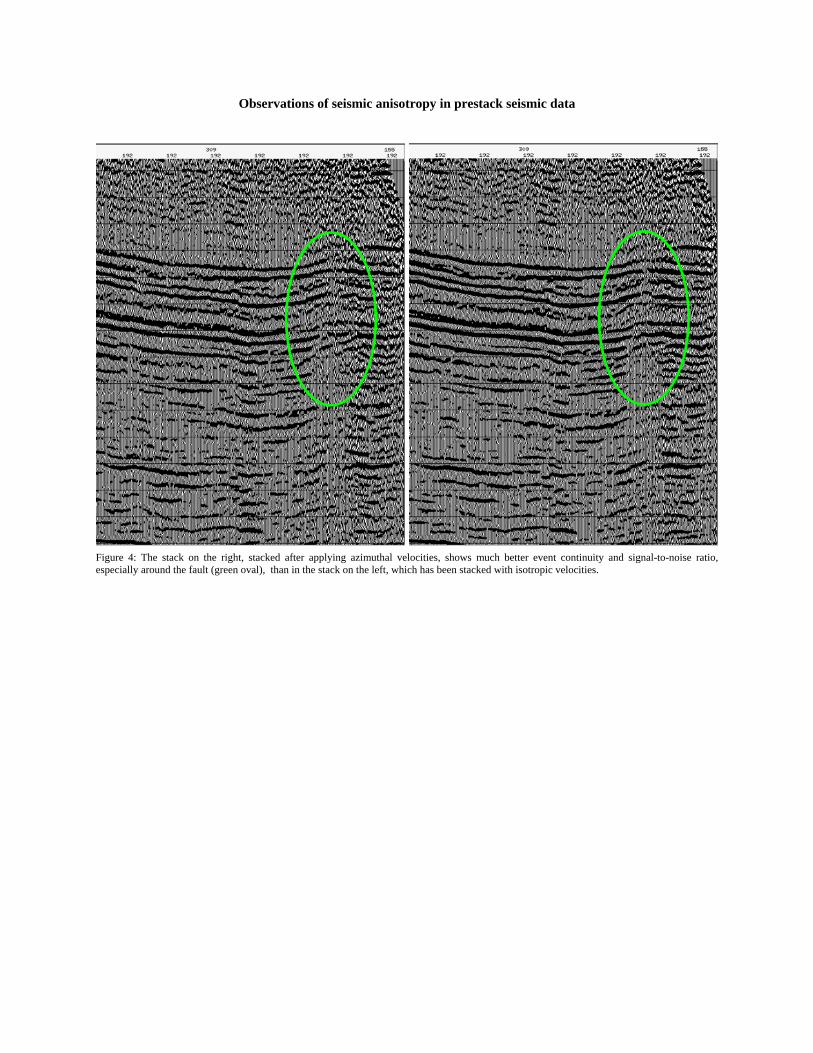
Figure 4: The stack on the right, stacked after applying azimuthal velocities, shows much better event continuity and signal-to-noise ratio, especially around the fault (green oval), than in the stack on the left, which has been stacked with isotropic velocities.