1

Observations of pigment and particle distributions in the Western North Atlantic from an autonomous float and ocean color satellite

E. Boss1,2, D. Swift3, L. Taylor2, P. Brickley2, R. Zaneveld4, S. Riser3, M.J. Perry5 and P. G.

Strutton6

2School of Marine Sciences, University of Maine, Orono, Maine 04469

3School of Oceanography, University of Washington, Seattle, Washington 98195-7940

4WET Labs, Inc., P.O. Box 518, 620 Applegate Street, Philomath, Oregon 97370

5Ira C. Darling Marine Center and School of Marine Sciences, University of Maine, Walpole,

Maine 04573

6College of Atmospheric and Oceanic Sciences, Oregon State University, Corvallis, Oregon

97331.

1 Corresponding author (emmanuel.boss@maine.edu).

2

Acknowledgments

This work was made possible with funding from the Ocean Biology and Biogeochemistry

Program of the National Aeronautics and Space Administration (NASA) under grant number

NAG5-12473. Discussions with Drs. F. Chai and M. Behrenfeld and comments by Dr. H.

Claustre and an anonymous reviewer are gratefully acknowledged.

3

Abstract Profiling floats with optical sensors can provide important complementary data to

satellite ocean color determinations by providing information about the vertical structure of

ocean waters, as well as surface waters obscured by clouds. Here we demonstrate this ability by

pairing satellite ocean color data with records from a profiling float that obtained continuous,

high-quality optical data for three years in the North Atlantic Ocean. Good agreement was found

between satellite and float data, and the relationship between satellite chlorophyll and float-

derived particulate backscattering was consistent with previously published data. Upper ocean

biogeochemical dynamics were evidenced in float measurements which displayed strong

seasonal patterns associated with phytoplankton blooms, and depth and seasonal patterns

associated with an increase in pigmentation per particle at low light. Surface optical variables

had shorter decorrelation time scales than did physical variables (unlike at low latitudes),

suggesting that biogeochemical rather than physical processes controlled much of the observed

variability. After 2.25 yr in the Subpolar North Atlantic between Newfoundland and Greenland,

the float crossed the North Atlantic Current to warmer waters, where it sampled an unusual eddy

for three months. This anticyclonic feature contained elevated particulate material from surface

to 1000m depth and was the only such event in the float's record. This eddy was associated with

weakly elevated surface pigment and backscattering, but depth-integrated backscattering was

similar to that previously observed during spring blooms. Such seldom-observed eddies, if

frequent, are likely to make an important contribution to the delivery of particles to depth.

4

Introduction Upper ocean processes have long been known to regulate the vertical distribution of

phytoplankton and the dynamics of blooms and primary production (e.g. Riley et al. 1949;

Sverdrup 1953; Denman and Gargett 1983; Smetacek and Passow 1990) through their influence

on nutrient and light availability. Unfortunately, estimating primary production (PP) from

shipboard observations at the temporal and spatial scales relevant to quantify the oceans' role in

global elemental cycling and climate is not practical.

Efforts have therefore been directed towards estimating primary production from

remotely observed ocean color. At this time, however, remotely sensed ocean color alone

cannot provide sufficiently accurate estimates of phytoplankton standing stocks and PP in the

upper ocean. The primary limitations are (1) no consensus exists regarding appropriate

algorithms for calculating PP and associated uncertainties, (2) ocean color data provide only

surface observations, so that estimates of subsurface distributions must rely on poorly

constrained assumptions, (3) satellites chronically undersample cloudy regions, and (4) the

atmosphere provides nearly 95% of the signal retrieved by the satellite, so very accurate

atmospheric correction schemes are required for reliable estimates of water-leaving radiance.

Since any biases in estimated PP and algal standing stock directly affect downstream estimates

of oceanic carbon budgets and fluxes, reducing uncertainties in ocean-color-based algorithms

will directly improve quantitative characterizations of global biogeochemical processes.

Profiling floats measuring physical parameters such as temperature and salinity have

been in operation since the late 1990s and are part of an international observation network (Argo,

e.g., Gould et al. 2004). However, very few profiling floats have been fitted with sensors that

monitor the ocean’s biogeochemistry. Recent effort has been devoted to pushing for the addition

of oxygen sensors to the Argo floats (Kortzinger et al. 2006). The float described in this paper

5

was equipped with optical sensors capable of providing estimates of the standing stock of

particles and phytoplankton chlorophyll a pigment.

Optical properties such as the diffuse attenuation coefficient and beam attenuation have

been previously measured with profiling floats (Mitchell et al. 2000; Bishop et al. 2002 & 2004)

to investigate the dynamics of phytoplankton and particulate organic materials in the upper ocean

for periods of up to eighteen months (Bishop et al., 2004). Bishop et al. (2002) used dusk-to-

dawn changes in beam attenuation to estimate growth rates of phytoplankton in the upper ocean

and related those rates to dust deposition events in the North Pacific.

Here we showcase the use of a profiling float to routinely obtain observations of upper

ocean hydrographical and optical properties that can be linked to ocean color measurements, as

would be possible if such sensors were incorporated into an Argo-like program. In addition to

measuring algal and particulate carbon parameters throughout the year, such floats provide

measurements in cloudy conditions and can be used to interpolate missing remotely sensed data.

The floats also provide distributions of biogeochemical parameters as a function of depth.

Together with physical data collected by float and satellite sensors, some links between upper

ocean dynamics and biogeochemistry are studied.

6

Material and methods A Webb Research Corp. APEX float was fitted with a Sea-Bird Electronics SBE41 CTD

and a single-prototype, flat-faced digital WET Labs hockey-puck-sized sensor package that

included two sensors: one measuring side scattering at 880nm (WET Labs LSS, e.g. Baker et al.

2001) and the other measuring chlorophyll a fluorescence (470nm excitation, 680nm emission,

analogous to the commercially available WET Labs ECO fluorometer). The LSS was chosen

because it was deemed to be the most sensitive single-faced scattering sensor available at the

time and it had the ability to provide estimates of mass concentration of particles in the deep

ocean with an accuracy similar to that of beam transmissometers (Baker et al., 2001).

Chlorophyll fluorescence provides a proxy for chlorophyll concentration and standing stocks of

phytoplankton biomass (Cullen, 1982), and scattering provides a proxy for total particulate mass

and particulate organic carbon (Baker et al., 2001, Stramski et al., 2008).

The CTD was mounted at the top of the float and the optical package was mounted near

the bottom, facing approximately 45 degrees outwards from the downward direction to avoid

reflections from the float and sedimentation of particles onto the sensor face. An oxygen sensor

was also deployed on the float but failed within six months of launch; hence, O2 data are not

reported here. Sensors were integrated into the float using a Sea-Bird Electronics, Inc., Apf9a

controller. Before launch, the float and sensors were tested for pressure effects and endurance in

a pressure tank simulating 50 dive cycles to 1200m, with data recorded throughout.

Fluorometer calibration—The chlorophyll fluorescence sensor was calibrated in the lab

by the manufacturer with a suspension of spinach chloroplasts and by us with a diatom culture at

the University of Maine. Two vicarious field calibrations were also performed. The float's first

70 days of chlorophyll data were compared with those from three similar optical sensors

7

deployed on a Labrador Sea mooring in June 2004 (simultaneous with float deployment) and

calibrated with chlorophyll extracted from local waters. Three years of float chlorophyll data

were vicariously calibrated against NASA’s MODIS chlorophyll product.

Calibration provides two parameters for converting measured fluorescence counts to

estimated chlorophyll concentration: a dark signal measured in the absence of fluorescence and a

slope parameter describing a linear fit of fluorescence to chlorophyll. The dark signal was

established by following the manufacturer’s recommendation to cover the detector with black

tape and to immerse the instrument in water while recording the output signal. During simulated

dives in a pressure tank, dark counts varied between 24 and 28 counts (with a minimum of 19

and a maximum of 31 counts). The dark count value reported by the manufacturer was 28, and

the minimum we measured in the field was 23 counts. Given this variability, we used a dark

count of 25 in the calculations presented below, and we propagated an uncertainty of 6 counts in

the estimates of uncertainties. (For comparison, 1mg m-3 of chlorophyll equals 500 counts.)

The slope relating measured fluoresced intensity (minus the dark signal, in counts) to

chlorophyll concentration (in mg m-3), is inherently variable due to biological variability in

chlorophyll-normalized absorption and fluorescence quantum yield (Cullen, 1982). Further

uncertainty was introduced into our fluorescence-to-chlorophyll conversions by the fact that the

470nm excitation band associated with our sensor is not at the peak of chlorophyll absorption but

rather that of accessory pigments that are passing electrons to the chlorophyll (Perry et al., this

issue).

The manufacturer's regression slope for our fluorometer (9.2⋅10-3 mg chl m-3 count-1),

based on spinach chloroplasts as the calibration standard, differed from the slope obtained at the

University of Maine (10.8⋅10-3 mg chl m-3 count-1) with a diatom culture. Vicarious calibration

8

against the mooring sensors resulted in a lower slope (4.2⋅10-3 mg chl m-3 count-1, 40 match-ups,

correlation coefficient R=0.76), and regression with NASA’s MODIS chlorophyll product (see

below) resulted in an even lower slope (2⋅10-3 mg chl m-3 count-1, 221 match-ups, R=0.88). We

elected to use the MODIS slope in the calculations presented here but suggest that these values

may be biased low by as much as a factor of 2, with a minimal absolute uncertainty of +/-0.03

mg chl m-3 (NASA reports their product to have an average global uncertainty of 30%; see also

discussion in Perry et al., this issue).

LSS calibration—The light scattering sensor (LSS) was calibrated by the manufacturer

with both a turbidity standard (formazine) and polystyrene calibration beads (Duke Scientific)

while taking simultaneous measurements with a spectral beam transmissometer (WET Labs ac9).

The LSS sensor was designed to provide a robust estimate of mass concentration of particles

(turbidity); as such, it does not have a well-defined sampling volume or well-defined scattering

angle but instead collects light scattered from all angles, with maximal response to sidescattered

photons (Baker et al. 2001).

The LSS calibration provides two parameters: a dark signal measured in the absence of a

scattering substance and a slope parameter that relates the counts measured by the instrument

(minus the dark counts) to the concentration of the calibration standard (expressed in

nephelometric turbidity units, NTU, when calibrated against formazine or in m-1 when calibrated

against a beam attenuation meter or a backscattering sensor). The dark counts were estimated by

the manufacturer to be 41.8, and in our pressure tests they varied between 50 and 54. The lowest

value measured in the field was 59 counts. Since the pressure tests were done just prior to

deployment, we used the lab average of 51.8 counts as the dark count in the calculations

presented here, and we propagated an uncertainty of 10 counts.

9

The slope parameter determined using a beam transmissometer measuring attenuation at

650nm differed by a factor of 3 for the formazin (1.30⋅10-4 m-1 counts-1) and calibration bead

(3.21⋅10-4 m-1 counts-1) solutions. Two vicarious field calibrations were also performed. The

slope derived from calibration against three near-surface, bead-calibrated, 440nm backscattering

sensors (i.e., providing an estimate of bbp(440)) on the Labrador Sea mooring (1.48⋅10-5 m-1

counts-1; 40 match-ups, correlation coefficient R=0.64) differed by less than 10% from a

regression with inversion-derived estimates of satellite-measured backscattering (1.64⋅10-5 m-1

counts-1; 213 match-ups; see below for details of the ocean color processing). For our

calculations of mass concentrations of particles, we elected to use the MODIS (satellite) slope.

Theoretical considerations—i.e., Mie calculations using a Fournier-Forand analytical

phase function (Fournier and Jonasz, 1999); indices of refraction, n, varying from 1.05 to 1.15;

and a particulate size distribution with differential power-law slopes varying from 3.5 to 4.5,

(slopes from Stramski and Kiefer, 1991)—suggest that the ratio of particulate backscattering at

440nm to the scattering measured by the LSS at 880nm can vary from 0.2 to 0.56. This range of

ratios would be much smaller for samples in which the particle composition varies less widely

than in the theoretical calculations (e.g., for a population of near-surface organic particles).

Based on the factors detailed above, we estimate the uncertainties in the backscattering

coefficients reported here to be on the order of a factor of two, with an absolute uncertainty in

the backscattering coefficient at 440nm of 3⋅10-4 m-1. To put this in perspective we note that the

backscattering coefficient of pure seawater at 440nm is 5.0⋅10-3 (Twardowski et al., 2007).

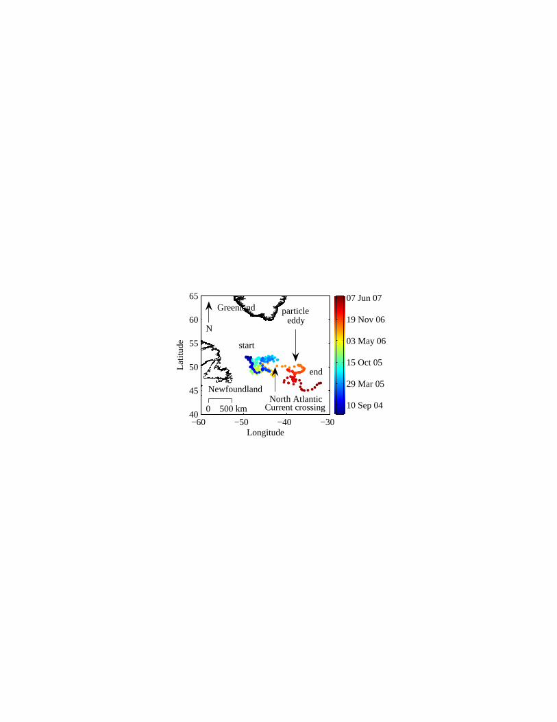
Float deployment and mission—The float, deployed at 51.84°N 48.43°W on 12 June

2004 (Fig. 1), was programmed to collect data every five days on an upward trajectory from

1000m depth to the surface. Data were collected at 50 depths during each profile, with larger

10

sampling intervals at depth and smaller intervals close to the surface. (Approximate data-

collection intervals were: over depth range 1000 to 450 m, every 50 m; over 400 to 325 m depth,

every 25 m; over 35 to 15 m depth, every 5m; and at 7 m below the sea surface). At the surface,

the CTD was turned off and in water measurements of chlorophyll fluorescence and

backscattering were taken while the float broadcast data to the Argos satellite.

To ensure that chlorophyll a fluorescence measurements were not biased by non-

photochemical quenching (e.g. Loftus and Seliger, 1975; Sackmann, 2007), the float was

programmed to surface close to midnight local time at the launch location. As the float drifted

approximately 17° of longitude westward over the course of its mission, the surfacing time was

always within two hours of the float's local midnight. After each profile, the float spent

approximately 10 hours at the surface, sending data to the Argos satellite (using an algorithm that

ensured that at least 95% of the data would be transferred) and collecting optical surface data

before returning to its parking depth at 1000m.

Satellite ocean color—Ocean color remote sensing products were obtained from

http://oceancolor.gsfc.nasa.gov/PRODUCTS/. For remotely sensed chlorophyll concentrations,

we used NASA’s OC3 standard chlorophyll product for the Moderate Resolution Imaging

Spectroradiometer (MODIS). For the remotely sensed particulate backscattering coefficient at

440nm (bbp(440)), we used normalized water-leaving radiances and the inversion algorithm

outlined in Maritorena et al. (2002). Level 2 data were processed as follows: all satellite passes

within a six-hour period (which amount to all data collected within a daylight period) were

averaged into a single scene. The data were subsequently median-averaged over all non-masked

data pixels within 7.5km of the float’s most recent location. (The 7.5km scale was based on a

11

spatial decorrelation analysis (not shown) and agrees with the local baroclinic radius of

deformation (e.g., Smith et al. 2000).) For vicarious calibration of the float's two sensors

(described above), the ocean color data were interpolated to the time of the float's surfacing (with

slightly fewer match-ups for backscattering than for chlorophyll: n=213 for bbp and n=221 for

chlorophyll).

We tested for contamination of pixels adjacent to clouds by applying a dilation operator.

Cloud-masked regions were enlarged by a binary dilation operation with a disk-shaped kernel

(two-pixel radius) to remove cloud edge effects (Gonzales and Woods, 1992). This operation

reduced the number of available remotely sensed spectra obtained for 12 June 2004 to 1 May

2007 from 233 to 150 without significantly changing either the correlation coefficient or the

calibration slope between in situ data and those inverted from satellite. We thus elected not to

apply the dilation procedure in the analyses that follow.

Sea surface height—Sea surface height anomaly data with ¼° resolution were obtained

from the Colorado Center for Astrodynamics Research at the University of Colorado, Boulder.

Data were processed as in Leben et al. (2002).

Results

Sensor stability and general oceanographic consistency—Float 0005 accomplished 221

profiles of the upper 1000m of the Western North Atlantic Ocean, one every five days, between

its launch on 12 June 2004 and its disappearance on 22 June 2007. The float spent most of its

mission in the Subpolar Gyre before crossing the North Atlantic Current (NAC) in September

12

2006 and drifting into warmer waters to the south (Fig. 1). The float then spent approximately 3

months within an anticyclonic eddy with highly elevated backscattering values (see below).

For one assessment of sensor stability, we examined data from depths greater than 970m,

with the expectation that in the absence of sensor drift, these deepwater values should remain

approximately consistent throughout the float mission. Except for rare spikes in the

backscattering coefficient (probably associated with occasional large particles entering the field

of view of the sensor) and the higher values associated with passage through an eddy, the deep

values are approximately constant (bbp(440)~0.00015m-1), suggesting that the float sensors were

stable over the course of the three-year mission (Fig. 2). The variability of the deep water

backscattering is on the order of 10% of the backscattering by pure seawater. Ultimately this is

the uncertainty when using the float data as validation for satellite derived backscattering values.

As a second assessment of sensor stability, we compared the float data to concurrent

satellite data. Although the remotely sensed data were earlier used to define the (single) slope

parameter we used to convert digital counts to estimates of chlorophyll and backscattering (see

methods), the consistent long-term correlation between surface estimates of these quantities

obtained from the satellite and from the float over three years supports our hypothesis of little

drift in the optical sensors (Fig. 3, correlation coefficient R=0.88 for chlorophyll and 0.90 for

backscattering, independent of the slope value chosen). If the float's sensors had experienced

significant instrumental drift, the satellite and float estimates of chlorophyll and backscattering

would have been expected to diverge over time.

The float data were also assessed in terms of their consistency with the relationships

between particulate backscattering and chlorophyll (Fig. 4) found in careful shipboard

measurements of in situ chlorophyll concentration and backscattering in the Antarctic Polar

13

Frontal Zone (APFZ), the Ross Sea (Reynolds et al. 2001), and the South Pacific (Huot et al.

2007). To convert bbp(555) reported in these studies to bbp(440) for this comparison, we assumed

a λ-1 spectral functionality for bbp and hence applied a multiplicative factor of 1.25. to the

bbp(555) values. Remotely sensed (satellite ocean color) estimates of backscattering and

chlorophyll are also included (Fig. 4; Behrenfeld et al. 2005). The float-based ratios of

backscattering to chlorophyll are consistent with those observed in these other studies.

Previous measurements were also available for suspended mass in the deep north Atlantic

(Jacob and Ewing, 1968). For this comparison, we relied on a regression between LSS-

determined turbidity and suspended matter (mg L-1; Baker et al. 2001) that is accurate to within

5%. Based on the manufacturer's LSS turbidity calibration translated in terms of backscattering,

suspended mass (in units of mg L-1) in our dataset is estimated to be approximately 20*bbp(440).

Applying this conversion factor to the float's measurements of backscattering in deep clear

waters (where bbp(440)~2⋅10-4 m-1, Fig. 2) provides an estimate of suspended mass of 0.004mg

L-1. This value is consistent with a previous report of 0.0045mg L-1 for clear deep North Atlantic

waters (Jacob and Ewing, 1968).

Upper ocean dynamics—To quantitively describe variability in the waters encountered

by the float, we calculated decorrelation time scales (a measure of how well correlated through

time are successive measurements of a given quantity) for both optical and physical float

measurements. Phytoplankton surface distributions are known to be spatially patchy (the local

baroclinic deformation radius and local spatial decorrelation scale of chlorophyll are O(10km))

and to have the potential to be highly variable temporally due to rapid growth rates (O(1 day)),

grazing dynamics, and mesoscale eddy dynamics. Thus one may expect chlorophyll data to be

14

highly uncorrelated between subsequent vertical profiles. Contrary to this expectation, however,

we find chlorophyll to have an unexpectedly long e-folding time of nearly two weeks (Fig. 5).

The near-surface optical properties (and thus biogeochemistry) have shorter decorrelation time

scales than do the physical properties (Fig. 5), with chlorophyll's being the shortest.

The float spent a little more than two years in the Subpolar Western North Atlantic (Fig.

1). The annual cycle dominates the variability in the sensor record, with surface waters warming

(decreasing in density) between February and late August, followed by subsequent cooling (Fig.

6). The near-surface chlorophyll and backscattering coefficients, which are always higher than

the same measurements at depth, exhibit a rapid rise in the spring and a slower decrease in the

fall and winter. The chlorophyll and backscattering coefficients are well correlated (R>0.86) in

the upper 300m, consistent with backscattering being dominated by phytoplankton and particles

that covary with phytoplankton (Fig. 4).

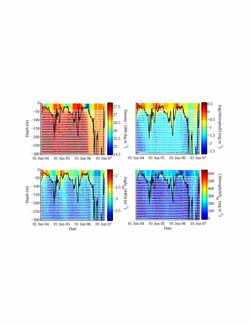
Significant variations in the chl/bbp ratio are observed in the course of the annual cycle

(Fig. 6). Below the mixed layer in the summer, a significant increase in chl/bbp is evident,

consistent with photoacclimation of cells to low light and/or availability of nutrients (Fig. 6).

This ratio also increases near the surface in the winter, possibly due to an increase in

pigmentation associated with short daylength and deeper mixing. When converting the upper

50m water-column bbp(440) to phytoplankton carbon using the conversion of Behrenfeld et al.

(2005), we find the chl/carbon ratio to have a median of 0.02 mg chl mg C-1 (10th percentile =

0.01, 90th percentile = 0.36), consistent with values observed in phytoplankton cultures (e.g.

Clohern et al., 1995).

At greater depths, no significant pigment concentration is observed at any time of year

(Fig. 7). In contrast, the seasonal modulation in backscattering is observed all the way to the

15

deepest depth bin (750-1050m), though with an amplitude two orders of magnitude smaller than

at the surface and a with maximum that is shifted later in the year relative to the surface’s

particle-concentration maximum.

Effects of clouds—To assess the usefulness of the float’s ability to sample under clouds, we

compared the temporal coverage provided by the float (5-6 surfacings per month) to that of the

MODIS satellite (Fig. 8) within the 7.5km radius around the float’s latest position. In summer

months, we obtained denser sampling with the remote sensing data; during the cloudy North

Atlantic winters, the float data density was superior.

To determine whether the greater winter data density from the float translates to

significantly different monthly mean values, we computed the coefficient of variation (the ratio

of the monthly standard deviation to the monthly mean) for the float chlorophyll data (Fig. 8).

During cloudy periods (when the number of satellite samples is low), the coefficient of variation

in optical properties is usually also low, indicating little change in upper ocean chlorophyll over

the course of the month. Sunny periods, associated with many remote observations, are usually

associated with a large coefficient of variation in upper ocean chlorophyll. This variance,

however, is often resolved by the more frequent satellite ocean color measurements.

The eddy event—An unusual eddy was sampled in the fall of 2006, following the float's crossing

of the North Atlantic Current. This eddy was quasi-stationary from September to mid-November

(not shown), had a small expression in remotely sensed chlorophyll concentration (relative to

measurements before and after its encounter, Fig. 3), and was observed well in altimetry data

(Fig. 9). While circling with the eddy, the float recorded the only occasion of deep ( > 970 m)

16

scattering significantly elevated above background levels (Fig. 2). Depth-integrated chlorophyll

values show little signal associated with the eddy; however, integrated bbp values show a signal

comparable in magnitude to that observed during the spring bloom (Fig. 10).

17

Discussion

We have demonstrated the ability to reliably measure optical variables—specifically,

chlorophyll concentration and particulate backscattering—for a period of three years with a

profiling float. Data quality was maintained with no apparent evidence of fouling, possibly due

to the mission profile, which included a large fraction of time in the dark, cold deep ocean and

relatively short stays at the surface (about ten hours every five days, mostly at night; see also

Bishop, 2002). The vicarious calibration approach performed here provides a chlorophyll to bbp

relationship consistent with those observed in other studies (Fig. 4). Average suspended mass

was also consistent with that previously observed in the deep north Atlantic.

Good temporal correlation between float-based and remotely sensed observations

showcases the potential for using similar inwater sampling platforms for validation and/or

interpolation of ocean color data. In addition, these data can be used to test for potential biases in

monthly mean satellite values during times of cloudy conditions. Here we find that within the

Subpolar Gyre, periods of sparse satellite coverage (i.e., winter) are correlated with low

variability in chlorophyll, suggesting that at high latitudes winter clouds do not significantly bias

remotely estimated monthly means. This result may be explained by the fact that the winter

period is associated with low temperatures and lower average mixed-layer light levels, both of

which are likely to decrease phytoplankton growth rates.

Autocorrelation analysis of the whole data set shows chlorophyll to have a shorter

decorrelation time scale than backscattering. This difference is likely due to the ability of

phytoplankton to rapidly (within a generation time scale) alter their intracellular chlorophyll

concentration in response to changes in light and nutrients, while other phytoplankton

components (phytoplankton carbon, for example) vary more slowly. The longer decorrelation

18

time scale for backscattering may also suggest that the scattering sensor is detecting slowly

varying material that does not covary with phytoplankton (e.g. some bacteria).

The chlorophyll decorrelation time scales observed by the float (O(20 days)) are

significantly longer than the O(2 days) decorrelation time scales calculated for equatorial Pacific

chlorophyll from ocean color data (Strutton and Chavez 2003) and the O(4 days) decorrelation

time scale calculated for California Current in situ chlorophyll from drifters (Abbott and Letelier,

1998). This result may seem surprising given the shorter deformation radius in the North

Atlantic, but can be explained by the significantly larger seasonal signal there. This signal

dominates the observed variability.

In comparing decorrelation time scales for optical variables and hydrographic variables,

we found shorter decorrelation time scales for all of the optical variables. Denman and Abbott

(1994) and Abbott and Letelier (1998), in contrast, observed equal decorrelation time scales for

temperature and chlorophyll in the California current. Strutton and Chavez (2003) interpret

covariation in decorrelation time scales as being a sign of causality. Under that interpretation, our

observation suggests that phytoplankton concentration in the Western North Atlantic is

significantly modulated by processes other than those responsible for variability in the upper

ocean’s hydrography.

One distinctive event captured by the float was a particle-rich eddy sampled in the late

fall of 2006 just south of the North Atlantic Current. This eddy's particle load was observed

coherently throughout the upper the 1000m of the water column, suggesting that it may be

responsible for a large flux of particles to depth. This event, which had little expression in

surface ocean color, is reminiscent of observations at the Bermuda Atlantic Time Series (BATS)

station (Conte et al. 2003) where, during some winters, large fluxes of biogenic materials were

19

collected in 3000m sediment traps in association with an eddy feature with little surface

expression in chlorophyll.

Currently we do not have a mechanism to explain the processes that formed or

concentrated the particulate material within the eddy. Settling velocities of micron-size particles

such as coccoliths cannot explain the temporal coherence in signal between near-surface

measurements and those at 1000m (B. Balch, 2007, personal communication). Additionally, no

anomalous atmospheric transmission values, possibly associated with a dust deposition event,

occurred during that time.

Eddies such as that sampled by the float and those observed at BATS could be very

important (even dominant) in the global biogeochemical inventory of carbon and its flux to depth

(e.g. Sweeney et al. 2003). However, we cannot currently account for such contributions due to

the faint ocean color signal of such eddies, our inability to sample the subsurface ocean from

space, and the limited space and time scales observable using shipboard observations or single-

point moorings, which cannot capture many realizations of such eddies.

In terms of methodological considerations, we found that care must be taken to ensure

that floats surface at nighttime. We had programmed midnight surfacings so as to avoid the

confounding effects of non-photochemical quenching in the chlorophyll fluorescence data.

Indeed, we often observed reductions in fluorescence through time after sunrise. A similar effect

has often been observed with fluorometers deployed on other autonomous vehicles such as

gliders (Perry et al., this issue).

In future deployments of optical floats, we would recommend replacing the sidescattering

sensor with a backscattering or attenuation sensor. The LSS, while excellent for quantifying

particles, has an optical geometry that is not very well constrained; this means that an LSS and

20

another optical sensor calibrated with the same calibration particles will likely give different

estimates of concentration in field samples where particle size and composition differ from those

of the calibration particles (e.g. Gibbs, 1974). In recent years, backscattering sensors that sample

a small, well-defined volume have been developed, providing an opportunity to measure an

inherent optical property (IOP) that is rather well understood and can be directly related to

remotely sensed quantities (Stramski et al., 2004). Backscattering is also a good proxy for

particulate organic carbon (e.g. Bishop 1999, Stramski et al. 2008).

Attenuation is another good proxy for particulate carbon (e.g., Bishop 1999, Stramski et

al. 2008), but our eddy experience points to a need for caution in field calibrations of beam

transmissometers. These instruments are often calibrated against the clearest deep waters in a

deep cast (e.g. Bishop et al. 2002, Stramski et al. 2008, and references therein). If, however, such

a procedure had been used in this North Atlantic study, the particle-signal increase associated

with the 2006 eddy would have been greatly reduced.

For future deployments, we would also recommend replacing the chlorophyll fluorometer

with a sensor to directly measure chlorophyll absorption (if a stable sensor could be developed).

Here we used chlorophyll fluorescence as a proxy for chlorophyll concentration, which, for

many processes and modeling studies, must in turn be converted to phytoplankton absorption.

The relationship between chlorophyll fluorescence and chlorophyll concentration is inherently

variable due to biological variability in chlorophyll-normalized absorption (a function of cell size

and accessory pigments) and fluorescence quantum yield (a function of species, nutritional

status, and light history). For example, calibration of a fluorescence sensor with the same

excitation and emission characteristics as ours found that calibration slopes (chl:F) for a marine

diatom specie and for a marine cyanobacterium differed by a factor of 7 (L. Karp-Boss

21

unpublished; see also Schubert et al. 1989). As a result, fluorescence—while a very useful proxy

for chlorophyll concentration, given that quantity's large dynamic range in oceanic waters—does

not give a very accurate measure of that concentration (Cullen, 1982, ACT report 2005).

If a chlorophyll fluorometer is to be used, it is advisable to perform the instrument's

prelaunch calibration using chlorophyll extracted from phytoplankton populations local to the

float's mission area. Better yet would be local-assemblage calibrations conducted at intervals

throughout the mission as often as possible. Even these extra-effort calibrations will fall short of

ideal because phytoplankton assemblages change with time and depth, but the more closely the

calibration standards can be matched to the local assemblage, the better. In addition, a recent

study using a novel optical sensor with multiple excitation-emission bands suggests the

possibility to significantly improve the accuracy of retrieved chlorophyll concentration (Proctor,

2008).

For future deployments of optical and biogeochemical sensors on floats or other

platforms, we also recommend that rigorous, quantitative error analysis and propagation be a

standard part of the calibration and data analysis procedures. We devoted considerable effort to

this undertaking (see methods), demonstrating that the fluorometer and LSS measurements are

accurate but imprecise. Fluorescence is an inherently noisy proxy for chlorophyll, but, again,

because of chlorophyll's large dynamic range in oceanic environments, even an imprecise

measurement is a useful one.

The quantification of analytical precision (see methods section) is not commonly

undertaken for optics-based methods used to characterize biogeochemical quantities—but it is

critically important. Ecosystem and biogeochemical ocean modelers are starting to use optical

variables to better model the underwater light field (e.g., for rate calculations of photosynthesis

22

and photooxidation) and to constrain biogeochemical variables (e.g. Fujii et al. 2007). Data such

as those collected by the float discussed here can provide these models with much-needed

groundtruth, resulting in increased model skill. Such exercises require, in addition to the basic

dataset, accompanying estimates of methodological and data uncertainties. Otherwise, the

propagation of errors throughout the model calculations and "goodness of fit" between model

output and observations cannot be quantitatively assessed.

In the very near future, O(5 yr), increasing numbers of biogeochemical modelers will

undoubtedly begin assimilating and testing against optical and other biogeochemical data sets.

However, the accompanying demand for high temporal and spatial high-quality optical data will

not be met by existing programs and platforms. In this study, we have demonstrated the

significant contribution that could be made by autonomous profiling floats (see also Uz, 2006). If

a fleet of biogeochemical profiling floats were to operate throughout the world’s oceans, the

contribution of the mesoscale band to important biogeochemical fluxes could be constrained.

Such a fleet (Argo) already exists for measurements of temperature and salinity. A

coordinated effort by the oceanographic community, analogous to the current effort to add

oxygen measurements, could make a complementary biogeochemical fleet a reality. All these

future float missions will benefit considerably from newer communication technologies such as

satellite cell phones (e.g. iridium), which allow for significantly shorter stays at the surface (less

than ten minutes), two-way communication (allowing for adaptive sampling), and higher vertical

sampling resolution per unit power.

It is our hope that the success and results demonstrated here and in previous optics-based

studies of ocean biogeochemistry (e.g. Bishop et al. 2002, 2004) will encourage the addition of

biogeochemical sensors to the existing and planned fleet of autonomous platforms in the world’s

23

oceans. Such a fleet could provide required inputs and constraints for the ocean-scale models

needed to improve our understanding of the oceans' roles in biogeochemical cycling in general

and of recent climate processes in particular.

References

ACT, 2005. Workshop proceedings on ‘Applications of in situ fluorometers in nearshore waters.'

Alliance for Coastal Technologies indexing No. ACT-05-03.

Abbott, M. R. and R. M. Letelier. 1998. Decorrelation scales of chlorophyll as observed from

bio-optical drifters in the California Current. Deep-Sea Res. II, 45, 1639-1667.

Baker, E. D., A. Tenant, R. A. Feely, G. T. Lebon, and S. L. Waker. 2001. Field and laboratory

studies on the effect of particle size and composition on optical backscattering measurements in

hydrothermal plumes. Deep-Sea Res. I 48: 593–604.

Behrenfeld, M.J., E. Boss, D.A. Siegel, and D.M. Shea, 2005. Carbon-based ocean productivity

and phytoplankton physiology from space. Global Biogeochemical Cycles 19 GB1006

10.1029/2004GB002299.

Bishop, J.K.B. 1999. Transmissometer measurement of POC. Deep-Sea Res. I. 46: 353-369.

Bishop, J.K.B., R.E. Davis, and J.T. Sherman. 2002. Robotic observations of dust storm

enhancement of carbon biomass in the North Pacific. Science 298: 817-821.

Bishop, J.K.B., T.J. Wood, R.E. Davis, and J.T. Sherman. 2004. Robotic observations of

enhanced carbon biomass and export at 55S. Science 304: 417-420.

24

Cloern, J. E., C. Genz, and L. Vidergar-Lucas. 1995. An empirical model of phytoplankton

chlorophyll: carbon ratio - the conversion factor between productivity and growth rate. Limnol.

Oceanogr. 40: 1313–1321.

Conte, M.H., T.D. Dickey, J.C. Weber, R. Johnson, and A. Knap. 2003. Transient physical

forcing of pulsed export of bioreactive material to the deep Sargasso Sea. Deep-Sea Res. I 50:

1157-1187.

Cullen, J. J. 1982. The deep chlorophyll maximum: comparing vertical profiles of chlorophyll a.

Can. J. Fish. Aquat. Sci. 39: 791-803.

Denman, K. L., and A. E. Gargett. 1983. Time and space scales of vertical mixing and advection

of phytoplankton in the upper ocean. Limnol. Oceanogr. 28: 801-815.

Denman, K. L. and M. R. Abbott. 1994. Time scales of pattern evolution from cross-spectrum

analysis of advanced very high resolution radiometer and coastal zone color scanner. J.

Geophys. Res. 99: 7433-7442.

Eppley, R. W. 1972. Temperature and phytoplankton growth in the sea. Fish. Bull. 70: 1063-

1085.

Fujii, M., Boss, E., and Chai, F. 2007. The value of adding optics to ecosystem models: a case

study, Biogeosciences, 4: 817-835.

Fournier G. and M. Jonasz. 1999. Computer-based underwater imaging analysis, in Airborne and

In-water Underwater Imaging, G. Gilbert, ed., Proc. SPIE 3761: 62–77.

Gibbs, R. J. [Ed.]. 1974. Suspended solids in water. Marine Science Ser. 4. Plenum Press,

New York and London.

25

Gonzalez, R.C. and R.E. Woods. 1992. Digital Image Processing. Addison-Wesley, Reading,

Massachusetts.

Gould, J., et al. 2004. Argo profiling floats bring new era of in situ ocean observations. Eos

Trans. AGU 85(19): 185.

Huot, Y., A. Morel, M.S. Twardowski, D. Stramski, and R.A. Reynolds. 2007. Particle optical

backscattering along a chlorophyll gradient in the upper layer of the eastern South Pacific Ocean,

Biogeosciences Discuss., 4: 4571-4604.

Jacobs, M. B., and M. Ewing. 1968. Suspended particulate matter: concentration in the major

oceans. Science 163: 380-383.

Körtzinger, A., S. C. Riser, and N. Gruber. 2006. Oceanic oxygen: the oceanographer's canary

bird of climate change. Argo Newsletter Argonautics 7 June 2006: 2-3.

Leben, R. R., G. H. Born, and B. R. Engebreth. 2002. Operational altimeter data processing for

mesoscale monitoring. Marine Geodesy 25: 3-18.

Loftus, M. E. and H. H. Seliger. 1975. Some limitations of the In vivo fluorescence technique.

Chesapeake Science 16: 79-92. doi:10.2307/1350685

Maritorena S., D.A. Siegel, and A. Peterson. 2002. Optimization of a semianalytical ocean color

model for global-scale applications. Appl. Opt. 41: 2705-2714.

Mitchell, B.G., M. Kahru, and J. Sherman. 2000. Autonomous temperature-irradiance profiler

resolves the spring bloom in the Sea of Japan. Proceedings, Ocean Optics XV, Monaco, October

2000.

26

Perry, M. J., B. S. Sackmann, C. C. Eriksen and C. M. Lee. 2008. Seaglider observations of

blooms and subsurface chlorophyll maxima off the Washington coast, USA. Limnol. Oceanog.

Submitted.

Proctor, C. 2008. Characterizing the calibration and sources of variability in a new sensor

package: using fluorescence to estimate phytoplankton concentration and composition. M.Sc.

thesis, Univ. of Maine.

Reynolds, R. A., D. Stramski, and B. G. Mitchell. 2001. A chlorophyll-dependent semianalytical

reflectance model derived from field measurements of absorption and backscattering coefficients

within the Southern Ocean. J. Geophys. Res. 106: 7125–7138.

Riley, G.A., H. Stommel, and D.F. Bumpus. 1949. Quantitative ecology of the plankton of the

Western North Atlantic. Bull. Bingham Oceanogr. Coll. 12(3): 1-169.

Sackmann, B.S. 2007. Remote assessment of 4-D phytoplankton distributions off the

Washington coast. Ph.D. dissertation, University of Maine (USA), 221 pp.

Schubert H., U. Schiewer, and E. Tschirner. 1989. Fluorescence characteristics of cyanobacteria

(blue-green algae). J. Plankton Res. 11: 353-359.

Smetacek, V., and U. Passow. 1990. Spring bloom initiation and Sverdrup's critical-depth

model. Limnol. Oceanogr. 35: 228-234.

Smith, R.D., M.E. Maltrud, F.O. Bryan, and M.W. Hecht. 2000. Numerical simulation of the

North Atlantic Ocean at 1/10°. J. Phys. Oceanogr. 30: 1532–1561.

Stramski, D., Kiefer, D.A. 1991. Light scattering by microorganisms in the open ocean. Progress

in Oceanography 28: 343-383.

27

Stramski, D., Boss E. , Bogucki D., and Voss K. J. 2004. The role of seawater constituents in

light backscattering in the ocean, Progress in Oceanography, 61, 27-55.

Stramski, D., Reynolds, R. A., Babin, M., Kaczmarek, S., Lewis, M. R., Röttgers, R.,

Sciandra, A., Stramska, M., Twardowski, M. S., and Claustre, H. 2008. Relationships between

the surface concentration of particulate organic carbon and optical properties in the eastern South

Pacific and eastern Atlantic Oceans, Biogeosciences, 5, 171-201.

Strutton, P.G. and F.P. Chavez. 2003. Scales of biological-physical coupling in the equatorial

Pacific. In L. Seuront and P.G. Strutton [eds.], Handbook of scaling methods in aquatic ecology.

CRC Press, Boca Raton, FL.

Sverdrup, H. U. 1953. On conditions for the vernal blooming of phytoplankton. J.

Conseil Exp. Mer. 18: 287.

Sweeney, E. N., D. J. McGillicuddy Jr., and K. O. Buesseler, 2003. Biogeochemical impacts due

to mesoscale eddy activity in the Saragasso Sea as measured at the Bermuda Atlantic Time-series

Study (BATS). Deep Sea Res. II 50: 3017-3039.

Twardowski, M. S., H. Claustre, S. A. Freeman, D. Stramski, and Y. Huot, 2007. Optical

backscattering properties of the "clearest" natural waters Biogeosciences, 4, 1041-1058.

Uz B. M. 2006. Argo floats complement biological remote sensing. EOS Transactions Vol.

87(32), 313-320.

28

Figure Legends

Fig. 1. Float trajectory.

Fig. 2. Potential temperature, salinity, particulate backscattering at 440nm, and chlorophyll at

depths deeper than 970m. The two vertical lines denote crossing of the North Atlantic Current

(left) and the center of a particle-rich anticyclonic eddy (right). Chlorophyll values lower than

0.04mg m-3 are not significantly different from zero.

Fig. 3. Time series and comparison of the particulate backscattering coefficient at 440nm and

chlorophyll concentration as measured by the float and satellite ocean color sensors.

Fig. 4. Particulate backscattering coefficient at 440nm vs. chlorophyll, as measured by the float

within the upper 10m (gray circles) and upper 300m (black circles) of the water column. Four

published relationships are also shown: Beh05, Behrenfeld et al. 2005; Rey01A, Reynolds et al.

2001, APFZ; Huo07, Huot et al. 2007, South Pacific; and Rey01R, Reynolds et al. 2001, Ross

Sea. Values of chlorophyll smaller than 0.04mg m-3 are not significantly different from zero.

Fig. 5. Lag correlation for near-surface chlorophyll, backscattering, density, salinity and

temperature measured from the profiling float. Temporal averages were removed from all

variables prior to computing the lag correlation.

Fig. 6. Evolution of density, chlorophyll and backscattering at 440nm and the ratio of

chlorophyll to backscattering at 440nm as a function of time and depth in the upper 300m. The

29

black line denotes the mixed layer depth (defined as the depth where density is 0.125kg m-3

greater than near the sea surface).

Fig. 7. Evolution of chlorophyll, density, particulate backscattering, and temperature as a

function of time for five depth bins. Lines represent the median of the property values for data in

the following depth bins: 0-30m, 75-130m, 185-245m, 315-480m, and 750-1050m. Each bin

contains approximately five sampling depths. The vertical black lines denote crossing of the

North Atlantic Current (left) and the center of a highly backscattering anticyclonic eddy (right).

Fig. 8. Number of data points per month provided by the float and satellite sensors, and

coefficient of variation of chlorophyll (based on float data) as a function of time.

Fig. 9. Float trajectory and backscattering coefficient from 5 September (49.8N, -39.4W) to 29

December 2006 (49.2N, -39,4W) overlain on contours of sea surface anomaly (in cm) for 18

October 2006. Note the anticyclonic eddy centered at 50N 37W. This feature was quasi-

stationary at this location for longer than two months.

Fig. 10. Integrated chlorophyll and particulate backscattering from the surface to 300m depth.

−60 −50 −40 −3040

45

50

55

60

65

Longitude

Latit

ude

10 Sep 04

29 Mar 05

15 Oct 05

03 May 06

19 Nov 06

07 Jun 07

0 500 km

N

NewfoundlandNorth Atlantic

Current crossing

Greenland

end

start

particleeddy

01 Jun 04 01 Jun 05 01 Jun 06 01 Jun 073

3.5

4

4.5

5

5.5

01 Jun 04 01 Jun 05 01 Jun 06 01 Jun 0734.8

34.85

34.9

34.95

35

35.05

35.1

Sal

inity

01 Jun 04 01 Jun 05 01 Jun 06 01 Jun 0710

−4

10−3

10−2

b bp(4

40)

(m−

1 )

Date01 Jun 04 01 Jun 05 01 Jun 06 01 Jun 07

0

0.01

0.02

0.03

0.04

0.05

Chl

orop

hyll

(mg

m−3 )

Date

Pot

entia

l tem

pera

ture

(o C)

10−1

100

101

10−1

100

101

Chlorophyll, MODIS

01 Jun 04 01 Jun 05 01 Jun 06 01 Jun 070

0.5

1

1.5

2

2.5

3

3.5

10−3

10−2

10−3

10−2

bbp

(440), MODIS

01 Jun 04 01 Jun 05 01 Jun 06 01 Jun 070

0.005

0.01

0.015

Date

Chl

orop

hyll,

AP

EX

float samplessatellite samples

Chl

orop

hyll

(mg −

3 )

b bp(4

40),

AP

EX

b bp(4

40)

(m−

1 )

10−1

100

10−4

10−3

10−2

b bp(4

40)

(m−

1 )

Chlorophyll (mg m−3)

Beh05Rey01aHuo07Rey01b

0 20 40 60 80 1000

0.2

0.4

0.6

0.8

1

Time lag (day)

Lag

cor

rela

tion

coef

fici

ent

tempsalσchlb

bp+ + +

01 Jun 04 01 Jun 05 01 Jun 06 01 Jun 07−300

−250

−200

−150

−100

−50

0

Dep

th (

m)

24.5

25

25.5

26

26.5

27

27.5

01 Jun 04 01 Jun 05 01 Jun 06 01 Jun 07

−2.5

−2

−1.5

−1

−0.5

0

0.5

01 Jun 04 01 Jun 05 01 Jun 06 01 Jun 07−300

−250

−200

−150

−100

−50

0

Date

Dep

th (

m)

−3.5

−3

−2.5

−2

01 Jun 04 01 Jun 05 01 Jun 06 01 Jun 07Date

0

100

200

300

400

500

600

Density−

1000 (kg m −3)

log(chlorophyll) (mg m −

3)

log(bbp (440)) (m−

1)

Chlorophyll/bbp (m

g m−

2)

01 Jun 04 01 Jun 05 01 Jun 06 01 Jun 070.003

0.03

0.3

3

Chl

orop

hyll

(mg

m−3 )

01 Jun 04 01 Jun 05 01 Jun 06 01 Jun 07

25

26

27

28

σ θ (kg

m−

3 )

01 Jun 04 01 Jun 05 01 Jun 06 01 Jun 0710

−4

10−3

10−2

b bp(4

40)

(m−

1 )

Date01 Jun 04 01 Jun 05 01 Jun 06 01 Jun 07

5

10

15

20

Tem

pera

ture

(o C)

Date

0−30 m75−130 m185−245 m315−480 m750−1050 m

01 Jun 04 01 Jun 05 01 Jun 06 01 Jun 070

5

10

15

20

25

Num

ber

of s

ampl

es p

er m

onth

Date

0

0.2

0.4

0.6

0.8

1

Coefficient of variation of float chlorophyll

CV of float chlorophyllfloat samplessatellite samples

Longitude (oW)

Latit

ude

(o N)

−42 −40 −38 −3648

48.5

49

49.5

50

50.5

51

−30

−20

−10

0

10

20b

bp= 0.3

bbp

= 0.9

cm

01 Jun 04 01 Jun 05 01 Jun 06 01 Jun 07

20

40

60

80

100

120

140

Dep

th in

tegr

ated

chl

orop

hyll

(mg

m−2 )

Date

0.2

0.4

0.6

0.8

1

1.2

1.4

Depth integrated bbp (440)

chlb

bp