Observational constraints to a phenomenological f (R,∇R)-model

R. R. Cuzinatto1∗, C. A. M. de Melo1,2†, L. G. Medeiros3‡, P. J. Pompeia4,5§

1Instituto de Ciencia e Tecnologia, Universidade Federal de Alfenas.Rod. Jose Aurelio Vilela (BR 267), Km 533, n11999, CEP 37701-970, Pocos de Caldas, MG, Brazil.

2Instituto de Fısica Teorica, Universidade Estadual Paulista.Rua Bento Teobaldo Ferraz 271 Bloco II, P.O. Box 70532-2, CEP 01156-970, Sao Paulo, SP, Brazil.

3Escola de Ciencia e Tecnologia, Universidade Federal do Rio Grande do Norte.Campus Universitario, s/n - Lagoa Nova, CEP 59078-970, Natal, RN, Brazil.

4Inst. de Fomento e Coordenacao Industrial, Departamento de Ciencia e Tecnologia Aeroespacial.Praca Mal. Eduardo Gomes 50, CEP 12228-901, Sao Jose dos Campos, SP, Brazil.

5 Instituto Tecnologico de Aeronautica, Departamento de Ciencia e Tecnologia Aeroespacial.Praca Mal. Eduardo Gomes 50, CEP 12228-900, Sao Jose dos Campos, SP, Brazil.

Abstract

This paper analyses the cosmological consequences of a modified theory of gravity whose actionintegral is built from a linear combination of the Ricci scalar R and a quadratic term in the covariantderivative of R. The resulting Friedmann equations are of the fifth-order in the Hubble function.These equations are solved numerically for a flat space section geometry and pressureless matter.The cosmological parameters of the higher-order model are fit using SN Ia data and X-ray gas massfraction in galaxy clusters. The best-fit present-day t0 values for the deceleration parameter, jerkand snap are given. The coupling constant β of the model is not univocally determined by the datafit, but partially constrained by it. Density parameter Ωm0 is also determined and shows weakcorrelation with the other parameters. The model allows for two possible future scenarios: theremay be either a premature Big Rip or a Rebouncing event depending on the set of values in thespace of parameters. The analysis towards the past performed with the best-fit parameters showsthat the model is not able to accommodate a matter-dominated stage required to the formation ofstructure.

Keywords: Gauge theory, Cosmic acceleration, Higher order gravity, Cosmology.PACS:98.80.-k, 11.15.-q.

1 Introduction

The cosmological constant is the simplest solution to the problem of the present-day acceleration ofthe universe. It is consistent with all the available observational tests, from the constraints imposedby CMB maps [1, 2] to BAO picks [3, 4] to SN Ia constraints [5, 6, 7, 8, 9] and the estimates of fractionof baryons in galaxy clusters through X-ray detection [10, 11]. Nevertheless, there is an uncomfortablefeeling from the fact that Λ is not satisfactory explained as a vacuum state of some field theory: theenergy scale observed for Λ and predicted by quantum field theory badly disagree [12]. This is one ofthe reasons why alternative explanations for the present-day cosmic acceleration have been put outsince 1998, when it was first detected [13, 14].

∗cuzinatto@gmail.com†cassius.anderson@gmail.com‡leogmedeiros@gmail.com§pedropjp@ifi.cta.br

1

arX

iv:1

311.

7312

v2 [

gr-q

c] 5

Dec

201

3

These proposals can be classified into two broad categories, each one related to a modification ofa different side of the Einstein field equations of General Relativity [15].

The modified matter approach introduces a negative pressure (that counteracts gravity) throughthe energy momentum tensor Tµν on the right-hand side of Einstein equations. Three types of modelsconstitute this approach, namely quintessence models [16, 17, 18, 19, 20], k-essence solutions [21, 22]and perfect fluid models (such as the Chaplygin gas [23, 24]). The quintessence and k-essence modelsare based on scalar fields whose potential (in the former case) or the kinetic energy (in the laterone) drive the accelerated expansion. The perfect fluid models use exotic equations of state (for thepressure as a function of the energy density) to generate negative pressure. The weakness of k-essenceand quintessence proposals lies in the fact that they require a scalar field to be dominant today, whenthe energy scale is low. This requirement demands the mass of such a field φ to be extremely small.One would then expect long range interaction of this field with ordinary matter, which is highlyconstrained by local gravity experiments. The difficulty with the perfect fluid models is the lack of aninterpretation to the exotic equations of state based on ordinary physics.

The second approach, called modified gravity, affects the left hand side of Einstein equations[25, 26]. The subtypes of models in this category include braneworld scenarios [27, 28], scalar-tensortheories [29, 30], non-riemannian geometries [31, 32, 33], f (R) gravity [34, 35, 36, 37, 38, 39] andf (T ) theories [40, 41, 42]. In the braneworld models there exists an additional dimension throughwhich the gravitational interaction occurs and by which the possibility of a cosmic acceleration isaccommodated. Scalar-tensor theories couple the scalar curvature R with a scalar field φ in the actionS, allowing enough degrees of freedom for an accelerated solution. Non-riemannian geometries areanother alternative way to explore the geometrization of the gravitational interaction, but allowingnew degrees of freedom describing different geometric structures than curvature. The f (R) gravitycorresponds to models resulting from non-linear Lagrangian densities dependent on R; f (T ) theoriesbuild their cosmological models on manifolds whose connection is equipped with torsion instead ofcurvature.

All these mechanisms of generating the present-day cosmic dynamics are generally called darkenergy models.

Our aim with the present paper is to contribute with the study of dark energy in the branch ofmodified gravity. We explore the cosmological consequences of a particular model in the context ofthe f (R,∇R) gravity testing the model against some of the observational data available. f (R,∇R)gravity is a theory based on an action integral whose kernel is a function of the Ricci scalar R andterms involving derivatives of R. Ref. [43] is perhaps an early example of what we call f (R,∇R)gravity. A more recent example is the (non-local) higher derivative cosmology presented in Refs.[44, 45, 46]. These works intend to eliminate the Big Bang singularity through a bounce produced bya theory based on an action containing the regular Einstein-Hilbert term plus a String-spired term.This last ingredient contains an infinite number of derivatives of R, a requirement needed to keep thismodified gravity theory ghost-free. References [47, 48] are f (R,∇R)-gravity prototypes concernednot with the past-incomplete inflationary space-time but with the cosmological constant problem. Inthis regard, they try to address a similar issue that interests us in the present work: the cosmologicalacceleration nowadays.

Few years ago, we proposed a gauge theory based on the second order derivative of the gaugepotential A following Utiyama’s procedure [49]. This led to a second field strength G = ∂F + fAF(depending on the field strength F ) and allowed us to obtain massive gauge fields among other ap-plications, such as the study of gauge invariance of the theory under U(1) and SU(N) groups whenL = L

(A, ∂A, ∂2A

). In a subsequent work, gravity was interpreted as a second order gauge theory

under the Lorentz group, and all possible Lagrangians with linear and quadratic combinations of Fand G – or the Riemann tensor, its derivatives and their possible contractions, from the geometricalpoint of view – were built and classified within that context [50]. In a third paper we selected oneof those quadratic Lagrangians for investigating the cosmological consequences of a theory that takesinto account R- and (∇R)2-terms [51]. That Lagrangian appears in the action S bellow – Eq. (1) –

2

and can be understood as a particular example of an f (R,∇R) gravity:

S =

∫d4x√−g(R

2χ+

β

8χ∇µR∇µR− LM

), (1)

where χ = 8πG (once we take c = 1), β is the coupling constant, ∇µ is the covariant derivative, andLM is the Lagrangian of the matter fields. As usual, g = det (gµν).1

An important feature of S is the presence of ghosts (see [46] and references therein). However,here this is not a serious issue because (1) should be considered as an effective action of a fundamentaltheory of gravity, this last one a ghost-free theory. There are some consistent proposals of extendedtheories of gravity in the literature. A good example is the String-inspired non-local higher derivativegravitation model presented in Ref. [45]. The ghost-free action of that model is:

S =

∫d4x√−g(M2P

2R+

1

2RF

(/M2

∗)R

)(2)

where MP is the Planck mass (MP = 1/ (8πG), G is the gravitational constant), M∗ is the mass scalewhere the higher-derivative terms become important and

F(/M2

∗)

=∞∑n=1

fnn . (3)

In this context, our higher-order model must be treated as a low energy limiting case of (2) wherethe only relevant contribution of Eq. (3) for the present-day universe is the first term of the series,i.e. f1 fn, ∀n > 2. In this approximation, Eq. (2) is equivalent to the action integral (1) of ourf (R,∇R)-cosmology up to a surface term. The equivalence of both models leads to a relation betweenthe coupling constant β and the parameter f1 ∼ M−2

∗ , namely

f1 =β

32πG. (4)

Taking the variation of (1) with respect to the metric tensor gµν (cf. the metric formalism) givesthe field equations

Rµν −1

2gµνR+ βHµν = χTµν , (5)

with

Hµν = ∇µ∇ν [R] +1

2∇µR∇νR

−RµνR− gµν [R]− 1

4gµν∇ρR∇ρR , (6)

where = ∇µ∇µ and Rµν is the Ricci tensor.A four dimensional spacetime with homogeneous and isotropic space section is described by the

Friedmann-Lemaıtre-Robertson-Walker (FLRW) line element

ds2 = c2dt2 − a2 (t)

[dr2

1− κr2+ r2

(dθ2 + sin2 θdφ2

)], (7)

where the curvature parameter κ assumes the values +1, 0,−1 and a (t) is the scale parameter. Sub-stituting the metric tensor from Eq.(7) along with the energy-momentum tensor of a perfect fluid inco-moving coordinates,

Tµν = (ρ+ P ) δ 0µ δ

0ν − Pgµν (8)

(ρ is the density and P is the pressure of the components fulling the universe), into the gravity fieldequations Eq.(5) leads to the two higher order Friedmann equations:

H2 +β

3F1 =

8πG

3ρ ; (9)

1The authors of Ref.[43] use the same action (1) proposed here but their argument is based on different motivations.

3

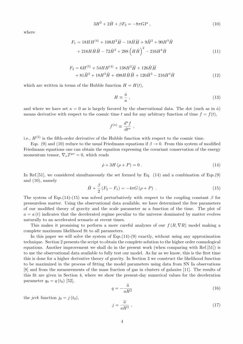
3H2 + 2H + βF2 = −8πGP , (10)

where

F1 = 18HH(4) + 108H2 ...H − 18H

...H + 9H2 + 90H3H

+ 216HHH − 72H3 + 288(HH

)2− 216H4H (11)

F2 = 6H(5) + 54HH(4) + 138H2 ...H + 126H

...H

+ 81H2 + 18H3H + 498HHH + 120H3 − 216H4H (12)

which are written in terms of the Hubble function H = H(t),

H ≡ a

a, (13)

and where we have set κ = 0 as is largely favored by the observational data. The dot (such as in a)means derivative with respect to the cosmic time t and for any arbitrary function of time f = f(t),

f (n) ≡ dnf

dtn,

i.e., H(5) is the fifth-order derivative of the Hubble function with respect to the cosmic time.Eqs. (9) and (10) reduce to the usual Friedmann equations if β → 0. From this system of modified

Friedmann equations one can obtain the equation expressing the covariant conservation of the energymomentum tensor, ∇νTµν = 0, which reads

ρ+ 3H (ρ+ P ) = 0 . (14)

In Ref.[51], we considered simultaneously the set formed by Eq. (14) and a combination of Eqs.(9)and (10), namely

H +β

2(F2 − F1) = −4πG (ρ+ P ) . (15)

The system of Eqs.(14)-(15) was solved perturbatively with respect to the coupling constant β forpressureless matter. Using the observational data available, we have determined the free parametersof our modified theory of gravity and the scale parameter as a function of the time. The plot ofa = a (t) indicates that the decelerated regime peculiar to the universe dominated by matter evolvesnaturally to an accelerated scenario at recent times.

This makes it promising to perform a more careful analyzes of our f (R,∇R) model making acomplete maximum likelihood fit to all parameters.

In this paper we will solve the system of Eqs.(14)-(9) exactly, without using any approximationtechnique. Section 2 presents the script to obtain the complete solution to the higher order cosmologicalequations. Another improvement we shall do in the present work (when comparing with Ref.[51]) isto use the observational data available to fully test our model. As far as we know, this is the first timethis is done for a higher derivative theory of gravity. In Section 3 we construct the likelihood functionto be maximized in the process of fitting the model parameters using data from SN Ia observations[8] and from the measurements of the mass fraction of gas in clusters of galaxies [11]. The results ofthis fit are given in Section 4, where we show the present-day numerical values for the decelerationparameter q0 = q (t0) [52],

q = − a

aH2(16)

the jerk function j0 = j (t0),

j =

...a

aH3, (17)

4

and also of the snap s0 = s (t0),

s =a(4)

aH4. (18)

These last two functions are given in terms of higher-order time derivatives of the scale factor and itis only natural that they show up here. In Section 4.2 we perform an investigation of the dynamicalevolution of the model, comparing its behaviour towards the past with the standard solutions for singlecomponent universes. Moreover, we show that our f (R,∇R)-model accommodates a future Big Ripor a Rebouncing scenario depending on the values of the coupling constant β. The Rebouncing eventis the point where the universe attains its maximum size of expansion and from which it begins toshrink. Our final comments about the features of our model and its validity are given in Section 5.

2 Higher order cosmological model

The solution of our higher-order model shall be obtained from the integration of the pair of Eqs.(9)and (14). The definitions

B ≡ H40β , (19)

andΩm (t) ≡ χρ

3H20

=ρ

ρc, (20)

enables us to express Eq. (9) asH2

H20

+B

3H60

F1 = Ωm (t) (21)

and the conservation of energy-momentum Eq.(14) as

Ωm + 3HΩm = 0 , (22)

which is readly integrated:

Ωm = Ωm0

(a0

a

)3. (23)

It is standard to take a0 = 1. Moreover, substituting the solution (23) into Eq. (21), leads to afifth-order differential equation in a:

1

H20

a2a4 +B

H60

F1 = Ωm0a3 (24)

with

F1 = 6a(5)aa4 − 6a(4)aa4 + 12a(4)a2a3

+ 3...a 2a4 + 18

...a aaa3 − 78

...a a3a2

− 6a3a3 − 39a2a2a2 + 78aa4a− 180a6 (25)

In order to solve Eq. (24), we define the non-dimensional variables

H ≡ a

H0= a

H

H0; (26)

Q ≡ HH0

= −aH2

H20

q ; (27)

J ≡ Q

H0= a

H3

H30

j ; (28)

S ≡ J

H0= a

H4

H40

s , (29)

5

which are related to the Hubble function, deceleration parameter, jerk and snap. In fact, when thesevariables are calculated at the present time, t = t0, they give precisely the well known cosmologicalparameters: H (t0) = H0 = a0 = 1, Q0 = −q0, J0 = j0 and S0 = s0. In the set of variables(26)-(29), one variable is essentially the derivative of the previous one, therefore they can be usedto turn the fifth-order differential equation Eq.(24) into five first order differential equations to besolved simultaneously. Following the Method of Characteristics, we choose the scale factor a as theindependent variable of the model (instead of the cosmic time t), obtaining the system

dHdz = − 1

(1+z)2QH

dQdz = − 1

(1+z)2JH

dJdz = − 1

(1+z)2SH

dSdz = −1

(1+z)2F3 (z;H, Q, J, S)

, (30)

with

F3 (z;H, Q, J, S) = −2S (1 + z) +SQ

H2

− 1

2

(J

H

)2

− 3JQ (1 + z)

H+ 13JH (1 + z)2

+Q3 (1 + z)

H2+

13

2Q2 (1 + z)2 − 13QH2 (1 + z)3

+ 30H4 (1 + z)4 +Ωm0

6B

(1 + z)

H2− 1

6B, (31)

where we have used the relationship between the redshift and the scale factor,

(1 + z) =1

a. (32)

The system of Eq.(30) is solved numerically, which is indeed a far more simpler task than dealingdirectly with Eq. (24). This leads to a function H (z) (essentially equal to a) for each set [M] =q0, j0, s0, B,Ωm0 of cosmological parameters. This function is used to obtain an interpolated functionfor the luminosity distance dL = dL (z, [M]) of our model – defined bellow – which is to be fitted tothe data from SN Ia observations and from f -gas measurements.

3 Fitting the model to the SN Ia and f-gas data

3.1 SN Ia data

In order to relate the proposed model to the observational data, one has to build the luminositydistance dL [15],

dL = (1 + z)

z∫0

dz

H (z)=

(1 + z)

H0

z∫0

dz

(1 + z) H (z). (33)

Our task is to solve the system Eq.(30) for obtaining H, then to integrate numerically the non-dimensional luminosity distance,

dh (z; [M]) =H0

cdL (z; [M]) , (c = 1) (34)

for each set of cosmological parameters [M] = q0, j0, s0, B,Ωm0.Function dh appears in the definition of the distance modulus,

µr = 5 log10 dh + 5 log10

(c

H0d0

), (35)

6

where d0 is the reference distance of 10 pc. Observational data give µr of the supernovae and theircorresponding redshift z.

According to the likelihood method the probability distribution of the data

LSNIa ([M] | zi, µri) = NSNIae−χ

2SNIa([M])

2 (36)

(NSNIa is a normalization constant) is the one that minimizes

χ2SNIa ([M]) =

∑i

(µri − 5 log dh (zi, [M])− 5 log10

(c

H0d0

))2

σ2µi + σ2

ext

, (37)

where σµi is the uncertainty related to the distance modulus µri of the i-th supernova. The dataset used in our calculations is composed with the 557 supernovae of the Union 2 compilation [8].Uncertainty σext is given by

σ2ext = σ2

µv + σ2lens , (38)

i.e., it is the combination of the error σv in the magnitude due to host galaxy peculiar velocities (oforder of 300 km s−1),

σµv =2.172

z

σvc

with σv = 300 km s−1 , (39)

and the uncertainty from gravitational lensing

σlens = 0.093z (40)

which is progressively important at increasing SN redshifts. Further detail can be found in Refs.[53, 54], for example.

3.2 Galaxy cluster X-ray data

Measurements of the fraction of the mass of gas in galaxy clusters in the X-ray band of the spectrumconstrain efficiently the ratio Ωb0

Ωm0and exhibit a lower dependence on the values of other cosmological

parameters [10, 11].2 According to Ref.[11], the mass fraction of gas fgas relates to Ωb0Ωm0

as

fΛCDMgas (z) =

KAγb (z)

1 + s (z)

(Ωb0

Ωm0

)[dΛCDMA (z)

dA (z)

]1,5

, (41)

where dA is the angular distance for κ = 0,

dA (z) =dL (z)

(1 + z)2 =1

(1 + z)

1

H0

z∫0

dz

(1 + z)H (z; [M]). (42)

The term dΛCDMA (z) is the angular distance for the standard ΛCDM model, for which Ωm0 = 0.3,

ΩΛ = 0.7 and H700 = 70 km s−1Mpc−1, i.e.

dΛCDMA (z) =

1

(1 + z)

1

H0

z∫0

dz[Ωm0 (1 + z)3 + ΩΛ

]1/2. (43)

The other factors in Eq. (41) are defined bellow:

• K is a constant due to the calibration of the instruments observing in X-ray. Following Ref.[11], we take K = 1.0± 0.1.

2Ωb0 = ρb/ρc is the non-dimensional baryon density parameter.

7

• Constant A measures the angular correction on the path of an light ray propagating in thecluster due to the difference between ΛCDM model and the model that we want to fit to thedata. Ref. [11] argues that for relatively low red-shifts (as those involved here) this factor canbe neglected, i.e. taken as A = 1.

• γ accounts for the influence of the non-thermal pressure within the clusters. According toRef.[11], one may set 1.0 < γ < 1.1. Our choice is γ = 1.050± 0.029.

• b (z) is the bias factor related to the thermodynamical history of the inter-cluster gas. Onceagain due to arguments given in Ref.[11], this factor can be modeled as b (z) = b0 (1 + αbz)where b0 = 0.83± 0.04 and −0.1 < αb < 0.1. We set αb = 0.000± 0.058.

• Parameter s (z) = s0 (1 + αsz) describes the fraction of baryonic mass in the stars.3 Ref. [11]

uses s0 = (0.16± 0.05)h1/270 and −0.2 < αs < 0.2. Here

h70 =H0

H700

, (44)

and we will set αs = 0.000± 0.115. Analogously to Eq.(44), we define

h =H0

(100 km s−1Mpc−1), (45)

that will be required bellow.

• The baryon parameter Ωb0 is set to

Ωb0h2 = 0.0214± 0.002 (46)

following the constraints imposed by the primordial nucleosynthesis on the ratio D/H [55].

The uncertainties in the set of parameters b0, s0,K,Ωb0h2, αs, αb, γ are propagated to build the

uncertainty of fΛCDMgas . It is worth mentioning that the quantities

b0, s0,K,Ωb0h

2

have Gaussianuncertainties. On the other hand, the parameters αs, αb, γ present a rectangular distribution, e.g.γ has equal probability of assuming values in the interval [1.0, 1.1]. The uncertainty of the parametersobeying the rectangular distribution is estimated as the half of their variation interval divided by

√3.

Maybe it is useful to remark that in the case of s0, we adopted h1/270 ' 1. Moreover, h2

h270=(

0.71

)2 ∼= 0.49.

Ref. [11] provides data for the fraction of gas fgas and its uncertainty σf of 42 galaxy clusters withredshift z. These data can be used to determine the free parameter of our model by minimizing

χ2gas ([M]) =

∑i

(f igas − fΛCDM

gas (z, [M]))2

σ2fi

(47)

Notice that the dependence of χ2 on the set [M] of cosmological parameters occurs through thefunction fΛCDM

gas given by Eq.(41), i.e. ultimately through dA (z, [M]) – Eq. 42.Function χ2

gas is related to the distribution

Lgas ([M]) = Ngase−χ2gas([M])

2 (48)

which should be maximized.

3Notice that here s0 is not the snap, defined in Eq. (18). Even at risk of confusion, we decided to maintain thenotation used in Ref. [11].

8

3.3 Combining SN Ia and f-gas data sets

The majority of papers that present cosmological models tested through SN Ia data fit – see e.g. Refs.[20, 53] – perform an analitical marginalization with respect to H0. On the other hand, constraintanalyses using f -gas data adopt a fixed value for H0. Our basic reference on f -gas treatment, namelyRef.[11], choose H0 = 70 km s−1Mpc−1. As we will consider SN Ia and f -gas data sets in the samefooting, it is convenient to adopt H0 = 70 km s−1Mpc−1 as a fixed quantity in our calculations (andnot the most up-to-date value of (73.8± 2.4) km s−1Mpc−1 found in [56]).

We want to maximize the probability distributions given in Eqs.(36) and (48) simultaneously,which is done by maximixing

L ([M]) = LSNIa ([M])Lgas ([M]) , (49)

or minimizingχ2 ([M]) = χ2

SNIa ([M]) + χ2gas ([M]) . (50)

4 Results

4.1 Estimation of the free parameters of the f (R,∇R)-model

The parameters to be ajusted are of two types. The kinematic parameters are q0, j0, s0;4 the cos-mological parameters are Ωm0, B. Maximization of the likelihood function L ([M]) – Eq. (49) –determines all kinematic parameters and one cosmological parameter, namely q0, j0, s0,Ωm0. Pa-rameter B is not fixed by statistical treatment of the data, and the reason for that is evident in theplot of Fig. 1.

The curve of L (|B|) is not Gaussian but rather shows a flat region at high values of |B|. Indeed,values of |B| greater than 10−3 are almost equally probable and more favorable than the |B| < 10−3.This shows it is not possible to determine B by maximizing its likelihood function. Instead, we choosefour values of B to proceed the analysis leading to the determination of the free parameters of themodel. These values are B =

(±10−3,±10−1

), so that we have two values of B in the beginning of

the plateau (|B| = 10−3) and two of them far from the beginning of the plateau (|B| = 10−1). Thesechoices are only partially arbitrary: we have done preliminary calculations with other values of |B|(|B| = 1, 10, 100) and the results for the best-fit calculations of q0, j0, s0,Ωm0 are almost the sameas those obtained by using |B| = 10−1.

The standard statistical analysis leads to the best-fit values of the parameters shown in Table 1.

Table 1: Fit results of the parameters of our f (R,∇R)-model. The uncertainties represent a 68%confidence level (CL).

B q0 j0 s0 Ωm0

−10−1 −0.51+0.14−0.14 0.3+1.7

−2.5 0.4+9.3−11.1 0.301+0.010

−0.010

−10−3 −0.55+0.14−0.14 1.4+2.1

−2.2 18.5+9.8−11.0 0.301+0.011

−0.010

+10−3 −0.46+0.14−0.14 −1.6+2.1

−2.1 −19.4+9.7−10.3 0.301+0.010

−0.010

+10−1 −0.51+0.14−0.14 0.3+1.7

−2.5 0.4+9.3−11.0 0.301+0.010

−0.010

It is clear from Table 1 that our higher order cosmological model presents an acceleration at presenttime: the deceleration parameter q0 is negative for all the values of the coupling constant B. This isa robust result indeed once we have got negative values for q0 with 99.7% confidence level.

Both SN Ia and f -gas data sets give information about astrophysical objects at relatively lowredshifts (z . 1.4). That is the reason for the high values of the uncertainties on the parameter j0 and

4We emphasize that q0, j0, s0 are precisely the values of −Q, J, S calculated at the present time t = t0.

9

1E-5 1E-4 1E-3 0.01 0.1-0.2

0.0

0.2

0.4

0.6

0.8

1.0

1.2

Like

lihoo

d Fu

nctio

n

|B|

Figure 1: Sketch of the likelihood function L ([M]) as a function of the absolute value of the couplingparameter B. The other parameters q0, j0, s0,Ωm0 were fixed in their best-fit values.

s0. Positive values of j0 mean that the tendency is the increasing of the rate of cosmic acceleration.Because the jerk parameter j0 does not exhibit the same sign for all values of B, it is not possibleto argue in favor of an overall behavior for the cosmic acceleration today. This statement is alsoapplicable to the snap s0 obtained with B = ±10−1. However, the uncertainties in the value of s0 forB = −10−3 do indicate that it is positive within 68% CL. The negative value of s0 for B = +10−3 isalso guaranteed within the same CL. This difference in the sign of s0 for B = −10−3 and B = +10−3

leads to distinct dynamics for the scale factor towards the future, as we shall discuss in Section 4.2.The best-fits for Ωm0 are statistically the same for all the chosen values of B. This is linked

to the fact that the f -gas data produce a sharp determination of this parameter. Notice that thevalue Ωm0 of our model is compatible with that of ΛCDM model as reported in Ref.[8] within 95%CL. Inspection of Table 1 indicates that the Gaussian-like distributions centered in each parameterof the set q0, j0, s0,Ωm0 for B = −10−1 overlap the distributions centered in q0, j0, s0,Ωm0 forB = +10−1; this overlap of distribution curves occurs within 68% CL of each distribution. Moreover,this overlap of distributions is greater than the one observed in the case of the sets q0, j0, s0,Ωm0for B = −10−3 and B = +10−3, which occurs within 95% CL. Hence, the greater the value of |B|,the greater the overlap of distribution and the less important is our choice of the value of B. Thisemphasizes what was said before about the choice of values for B.

The confidence regions (CR) in the (q0, j0) and (q0,Ωm0) planes for each one of the four values ofB are shown in Figs. 2-5.

The shape of the confidence regions for (q0, j0) indicates that the deceleration parameter q0 andthe jerk j0 are correlated parameters; this occurs for all the values of B. The four plots (q0, j0) point

10

-0.8 -0.6 -0.4 -0.2

0.27

0.28

0.29

0.30

0.31

0.32

0.33

q0

Wm

0

-0.8 -0.6 -0.4 -0.2

-6

-4

-2

0

2

4

q0

j 0

Figure 2: Confidence regions in the (q0,Ωm0) and (q0, j0) planes for B = −10−1 from SN Ia and f -gasdata sets. The inner contour contains the 68% CR, whilst the outer curves confines the 95% CR.

0.9 0.8 0.7 0.6 0.5 0.4 0.3 0.2

4

2

0

2

4

6

q0

j 0

-0.9 -0.8 -0.7 -0.6 -0.5 -0.4 -0.3 -0.2

0.27

0.28

0.29

0.30

0.31

0.32

0.33

q0

Wm

0

Figure 3: 68% and 95% confidence regions in the (q0, j0) and (q0,Ωm0) planes for B = −10−3.

11

0.8 0.6 0.4 0.2

8

6

4

2

0

2

4

q0

j 0

0.8 0.6 0.4 0.2

0.27

0.28

0.29

0.30

0.31

0.32

0.33

q0

m

0

Figure 4: Confidence regions in the plots (q0, j0) and (q0,Ωm0) planes for the value B = +10−3 of thecoupling constant.

-0.8 -0.6 -0.4 -0.2

-6

-4

-2

0

2

4

q0

j 0

-0.8 -0.6 -0.4 -0.2

0.27

0.28

0.29

0.30

0.31

0.32

0.33

0.34

q0

Wm

0

Figure 5: CR in the planes (q0, j0) and (q0,Ωm0) for B = +10−1.

12

to an accelerated universe at recent times within 95% CL, but the change in the acceleration ratetakes positive and negative values with equal probability.

Conversely, the shape of the plots of (q0,Ωm0) in Figs. 2–5 indicate that q0 and Ωm0 are weaklycorrelated parameters. Notice that the difference between the maximum and the minimum values ofΩm0 in the range of the plots q0 × Ωm0 is only 0.05 with 95% CL: this confirms that the parameterΩm0 is sharply determined by the best-fit procedure (something that is consistent with the fact thatwe have employed f -gas data to build the likelihood function).

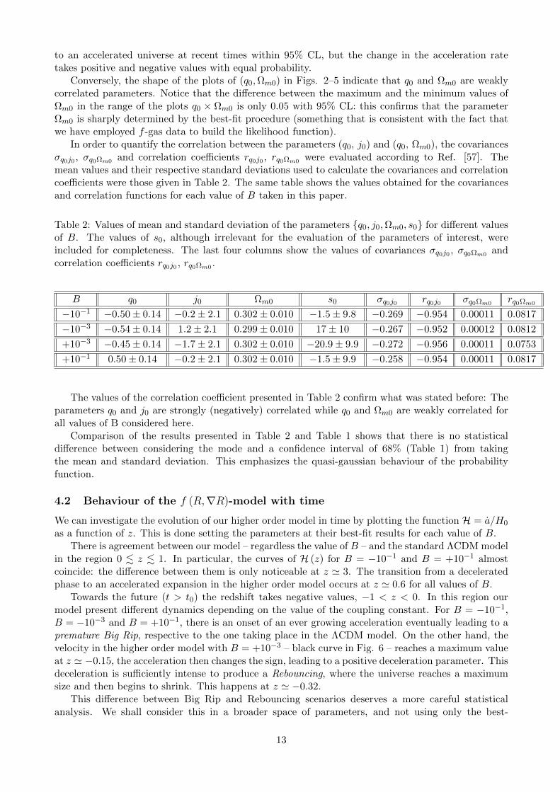
In order to quantify the correlation between the parameters (q0, j0) and (q0, Ωm0), the covariancesσq0j0 , σq0Ωm0 and correlation coefficients rq0j0 , rq0Ωm0 were evaluated according to Ref. [57]. Themean values and their respective standard deviations used to calculate the covariances and correlationcoefficients were those given in Table 2. The same table shows the values obtained for the covariancesand correlation functions for each value of B taken in this paper.

Table 2: Values of mean and standard deviation of the parameters q0, j0,Ωm0, s0 for different valuesof B. The values of s0, although irrelevant for the evaluation of the parameters of interest, wereincluded for completeness. The last four columns show the values of covariances σq0j0 , σq0Ωm0 andcorrelation coefficients rq0j0 , rq0Ωm0 .

B q0 j0 Ωm0 s0 σq0j0 rq0j0 σq0Ωm0 rq0Ωm0

−10−1 −0.50± 0.14 −0.2± 2.1 0.302± 0.010 −1.5± 9.8 −0.269 −0.954 0.00011 0.0817

−10−3 −0.54± 0.14 1.2± 2.1 0.299± 0.010 17± 10 −0.267 −0.952 0.00012 0.0812

+10−3 −0.45± 0.14 −1.7± 2.1 0.302± 0.010 −20.9± 9.9 −0.272 −0.956 0.00011 0.0753

+10−1 0.50± 0.14 −0.2± 2.1 0.302± 0.010 −1.5± 9.9 −0.258 −0.954 0.00011 0.0817

The values of the correlation coefficient presented in Table 2 confirm what was stated before: Theparameters q0 and j0 are strongly (negatively) correlated while q0 and Ωm0 are weakly correlated forall values of B considered here.

Comparison of the results presented in Table 2 and Table 1 shows that there is no statisticaldifference between considering the mode and a confidence interval of 68% (Table 1) from takingthe mean and standard deviation. This emphasizes the quasi-gaussian behaviour of the probabilityfunction.

4.2 Behaviour of the f (R,∇R)-model with time

We can investigate the evolution of our higher order model in time by plotting the function H = a/H0

as a function of z. This is done setting the parameters at their best-fit results for each value of B.There is agreement between our model – regardless the value of B – and the standard ΛCDM model

in the region 0 . z . 1. In particular, the curves of H (z) for B = −10−1 and B = +10−1 almostcoincide: the difference between them is only noticeable at z ' 3. The transition from a deceleratedphase to an accelerated expansion in the higher order model occurs at z ' 0.6 for all values of B.

Towards the future (t > t0) the redshift takes negative values, −1 < z < 0. In this region ourmodel present different dynamics depending on the value of the coupling constant. For B = −10−1,B = −10−3 and B = +10−1, there is an onset of an ever growing acceleration eventually leading to apremature Big Rip, respective to the one taking place in the ΛCDM model. On the other hand, thevelocity in the higher order model with B = +10−3 – black curve in Fig. 6 – reaches a maximum valueat z ' −0.15, the acceleration then changes the sign, leading to a positive deceleration parameter. Thisdeceleration is sufficiently intense to produce a Rebouncing, where the universe reaches a maximumsize and then begins to shrink. This happens at z ' −0.32.

This difference between Big Rip and Rebouncing scenarios deserves a more careful statisticalanalysis. We shall consider this in a broader space of parameters, and not using only the best-

13

-1.0 -0.5 0.0 0.5 1.0 1.5 2.0 2.5 3.00.0

0.5

1.0

1.5

2.0

2.5

3.0

H(z

)

z

B=-10-1

B=-10-3

B=10-3

B=10-1

CDM

Figure 6: Plot of the function H (z) accounting for the best-fit parameters of the higher order model.This is essentially the curve of a as a function of z for our model – colored lines – and for the standardΛCDM model – dashed line. The notation is: B = −10−1 is the blue curve; B = −10−3, red line;B = +10−3, black curve; and B = +10−1, green line.

fit values for the parameters of our model, as we have done so far. A careful analysis shows thatthe deceleration parameter q0 influences weakly on the possible future regimes of our model. Theparameters that decisively decide in favor of a Big Rip scenario or a Rebouncing event are the jerk j0and the snap s0. Fig. 7 displays the (j0, s0) confidence regions plots for B = ±10−1.

The straight red lines passing through the confidence regions of the plots Fig. 7 separate thesector of the space of parameters where the Rebouncing occurs (lower part) from that region of valuescorresponding to a Big Rip (upper part). A numerical analysis shows that 39% of the (j0, s0) confidenceregion allows for the Rebouncing scenario in the higher order model with B = −10−1 and 42% of theconfidence region for the model with B = +10−1 leads to Rebouncing. A similar analysis shows thatthe model with B = −10−3 produces a premature Big Rip for all the values of the pair (j0, s0) in the95% confidence region; converselly, the model with B = +10−3 engenders Rebouncing within the 95%CR.

At last, it is interesting to explore the features of the model for z & 1. Extrapolating the resultspresented in Fig. 6 we verified that our model does not reproduce the decelerated phase typical of amatter dominated Friedmann universe. Besides, for 10 . z . 1000 the higher order model exhibits abehaviour compatible with5

1

3< ω <

1.25

3, (51)

where the equation of state is P = ωρ, i.e. the equation for a perfect fluid in the standard Friedmanncosmology. On the other hand, a linear perturbative analysis shows that the perturbations in gravi-tation and matter fields do not grow for the equation of state with ω as given in (51). Therefore, themodel proposed here can not describe the structure formation in the early universe.

5 Final Remarks

In this paper we have studied the phenomenological features of a particular modified gravity modelbuilt with an action integral dependent on the Ricci scalar R and also on the contraction ∇µR∇µR of

5The result (51) is still valid even when radiation is added to the model.

14

-4 -2 0 2 4

-20

-10

0

10

20

j0

s 0

-4 -2 0 2 4

-20

-10

0

10

20

j0

s 0Figure 7: (j0, s0) confidence regions for B = −10−1 (left) and B = +10−1 (right) with q0 and Ωm0 setto their best-fit values.

its covariant derivatives. The Friedmann equations resulting from the field equation and the FLRWline element involve sixth-order time-derivatives of the scale factor a. We solved those differen-tial equations numerically – but without any approximation – assuming a null cuvature parame-ter (κ = 0) and pressureless matter. Our higher order model depends on five parameters, namely[M] = q0, j0, s0,Ωm0;B. The present day value of the Hubble constant is taken as given – and notconstrained by data fit – the reason for that being consistency with the f -gas data analysis. Four ofthe five parameters [M] are determined by the best-fit to the data for the SN Ia dL (z) and fractionof gas in galaxy clusters dA (z) available from Refs.[8] and [11], respectively.

The shape of the likelihood function L in terms of B shows that it is not possible to determine thisparameter by maximization. We were forced to select some values of B and proceed to the best-fitof the other parameters in the set [M]. It was clear that the Ωm0 is statistically independent of theinitial conditions, regardless the values of B and the other best-fit parameters. In addition the signof both j0 and s0 depend on B, so that the behaviour of the model towards the future is not unique.

The confidence regions for the pair of parameters (q0, j0), (q0,Ωm0) and (j0, s0) were built. Theyshowed that q0 and j0 are strongly correlated parameters, whereas q0 and Ωm0 are weakly correlatedquantities. This was confirmed by the results in Table 2. The plot of the confidence region for the pair(j0, s0) is relevant to understand the future evolution of our higher-order model, which can exhibiteither a premature Big Rip or a Rebouncing depending on the value of B and on the values of j0 ands0.

If additional data for high z objects were used, as Gamma Ray Bursts, for instance, they mightreduce the uncertainties in our estimations of the jerk and the snap, and help us to decide if theRebouncing scenario is favored with respect to the Big Rip, or conversely.

A positive feature of the particular f (R,∇R)-model presented here is its consistency with thestandard ΛCDM dynamics at recent times. Maybe this is anticipated because the model has a greatnumber of free parameters to be fit to the data. The high number of kinematic parameters (i.e.,those involving acceleration and its first and second derivatives) is a consequence of the model beingof the fifth-order in derivatives of H, a fact that could always make room for agreement with theobservations. However, the freedom for bias is not unlimited. Even with all these free parametersthere is a constraint to the dynamics of the model towards the past.

Besides this consistency with the standard ΛCDM dynamics (at recent times) the model does notreproduce a large scale structure formation phase. This shows that just fitting a model to actual data

15

is not enough to falsify or prove the model. General essential characteristic must be present too, asthe instabilities allowing the large scale structure formation. Therefore, the extra term presented inthe action (1) should be ruled out as viable alternative for dark energy.

Acknowledgements This paper is dedicated to Prof. Mario Novello on the ocasion of his 70thbirthday. RRC thanks FAPEMIG-Brazil (grant CEX–APQ–04440-10) for financial support. CAMMis grateful to FAPEMIG-Brazil for partial support. LGM acknowledges FAPERN-Brazil for financialsupport.

References

[1] D. N. Spergel et al., First year Wilkinson Microwave Anisotropy Probe (WMAP) observations:Determination of cosmological parameters, Astrophys. J. Suppl. 148 (2003), 175; E. Komatsuet al., Seven-year Wilkinson Microwave Anisotropy Probe (WMAP) observations: Cosmologicalinterpretation, Astrophys. J. Suppl. 192:18 (2011).

[2] Planck Collaboration: P. A. R. Ade et al., Planck 2013 results. I. Overview of products andscientific results, arXiv: 1303.5062 (2013); Planck Collaboration: P. A. R. Ade et al., Planck2013 results. XVI. Cosmological parameters, arXiv: 1303.5076 (2013).

[3] D. J. Eisenstein et al., Detection of the Barion Acoustic Peak in the large-scale correlation functionof SDSS luminous red galaxies, Astrophys. J. 633 (2005), 560; W. J. Percival et al., BaryonAcoustic Oscillations in the Sloan Digital Sky Survey Data Release 7 Galaxy Sample, Mon. Not.Roy. Astron. Soc. 401 (2010), 2148.

[4] S. Cole et al., The 2dF Galaxy Redshift Survey: Power-spectrum analysis of the final datasetand cosmological implications, Mon. Not. Roy. Astron. Soc. 362 (2005), 505; F. Beutler, The6dF Galaxy Survey: Baryon Acoustic Oscilations and the local Hubble constant, Mon. Not. Roy.Astron. Soc. 416 (2011), 3017.

[5] P. Astier et al., The Supernova legacy Survey: Measurement of ΩM , ΩΛ and w from the first yeardata set, Astron. Astrophys. 447 (2006), 31.

[6] A. G. Riess el al., Type Ia Supernova discoveries at z > 1 from the Hubble Space Telescope:Evidence for past deceleration and constraints on dark energy evolution, Astrophys. J. 607 (2004),665; A. G. Riess el al., New Hubble Space Telescope discoveries of Type Ia Supernovae at z > 1:Narrowing constraints on the early behavior of dark energy, Astrophys. J. 659 (2007), 98;

[7] W. M. Wood-Vasey et al., Observational constraints on the nature of the dark energy: firstcosmological results from the ESSENCE Supernova Survey, Astrophys. J. 666 (2007), 694.

[8] R. Amanullah et al., Spectra and Hubble Space Telescope light curves of six type Ia supervonaeat 0.511 < z < 1.12 and the Union2 Compilation, Astrophys. J. 716 (2010), 712.

[9] N. Suzuki et al., The Hubble Space Telescope Cluster Supernova Survey: V. Improving theDark Energy Constraints Above z > 1 and Building an Early-Type-Hosted Supernova Sample,Astrophys. J. 746 (2012), 85.

[10] S. Schindler, ΩM -different ways to determine the matter density of the universe, Space ScienceReviews 100 (2002), 299.

[11] S. W. Allen et al., Improved constraints on dark energy from Chandra X-ray observations of thelargest relaxed galaxy clusters, Mon. Not. Roy. Astron. Soc. 383 (2008), 879.

[12] S. Weinberg, The cosmological constant problem, Rev. Mod. Phys. 61 (1989) 1.

16

[13] A. G. Riess et al., Observational evidence from supernovae for an accelerating universe and acosmological constant, Astron. J. 116 (1998), 1009.

[14] S. Perlmutter et al., Measurements of Ω and Λ from 42 high-redshift supernovae, Astrophys. J.517 (1999), 565.

[15] L. Amendola e S. Tsujikawa, Dark Energy: Theory and Observations, Cambridge UniversityPress, New York (2010).

[16] B. Ratra and P. J. E. Peebles, Cosmological consequences of a rolling homogeneous scalar field,Phys. Rev D 37 (1988), 3406.

[17] R. R. Caldwell, R. Dave, and P. J. Steinhardt, Cosmological imprint of an energy componentwith general equation-of-state, Phys. Rev Lett. 80 (1998), 1582.

[18] S. M. Carrol, Quintessence and the rest of the world, Phys. Rev Lett. 81 (1998), 3067.

[19] A. Hebecker and C. Wetterich, Natural quintessence?, Phys. Lett. B 497 (2001), 281.

[20] L. Amendola, G. C. Campos, and R. Rosenfeld, Consequences of dark matter-dark energy inter-action on cosmological parameters derived from SN Ia data, Phys. Rev. D 75 (2007), 083506.

[21] T. Chiba, T. Okabe, and M. Yamaguchi, Kinetically driven quintessence, Phys. Rev. D 62 (2000),023511.

[22] C. Armendariz-Picon, V. F. Mukhanov, and P. J. Steinhardt, Essentials of k-essence, Phys Rev.D 63 (2001), 103510.

[23] A. Y. Kamenshchik, U. Moschella, and V. Pasquier, An alternative to quintessence, Phys. Lett.B 511 (2001), 265.

[24] M. C. Bento, O. Bertolami, and A. A. Sen, Generalized Chaplygin gas, accelerated expansionand dark energy-matter unification, Phys. Rev. D 66 (2002), 043507.

[25] S. Capozziello and M. De Laurentis, Extended theories of gravity, Phys. Rep. 509 (2011), 167.

[26] S. Nojiri and S. D. Odintsov, Unified cosmic history in modified gravity: from f (R) theory toLorentz non-invariant models, Phys. Rep. 505 (2011), 59.

[27] G. R. Dvali, G. Gabadadze, and M. Porrati, 4D gravity on a brane in 5D minkowski space, Phys.Lett. B 485 (2000), 208.

[28] V. Sahni and Shtanov, Braneworld models of dark energy, JCAP 0311 (2003), 014.

[29] N. Bartolo and M. Pietroni, Scalar tensor gravity and quintessence, Phys. Rev. D 61 (2000),023518.

[30] F. Perrota, C. Baccigalupi, and S. Matarrese, Extended quintessence, Phys. Rev. D 61 (2000),023507.

[31] Z. Chang, X. Li, Modified Friedmann model in Randers-Finsler space of approximate Berwaldtype as a possible alternative to dark energy hypothesis, Phys. Lett. B 676 (2009) 173.

[32] K. S. Adhav, LRS Bianchi Type-I Universe with Anisotropic Dark Energy in Lyra Geometry, Int.J. Astr. Astrophys., 1 No. 4, (2011) 204. doi: 10.4236/ijaa.2011.14026.

[33] R. Casana, C. A. M. de Melo, B. M. Pimentel, Massless DKP field in a Lyra manifold, Class.Quantum Gravity 24 (2007) 723.

[34] S. Capozziello, Curvature quintessence, Int. J. Mod. Phys. D 11 (2002), 483.

17

[35] A. De Felice and S. Tsujikawa, f (R) theories, Living Rev. Rel. 13 (2010), 3.

[36] T. P. Sotiriou and V. Faraoni, f (R) theories of gravity, Rev. Mod. Phys. 82 (2010), 451.

[37] J. Santos et al., Latest supernovae constraints on f (R) cosmologies, Phys. Lett. B 669 (2008),14.

[38] N. Pires, J. Santos and J. S. Alcaniz, Cosmographic constraints on a class of Palatini f (R) gravity,Phys. Rev. D 82 (2010), 067302.

[39] S. Nojiri and S. D. Odintsov, Introduction to modified gravity and gravitational alternative fordark energy, Int. J. Geom. Meth. Mod. Phys. 4 (2007), 115.

[40] G. Bengochea and R. Ferraro, Dark torsion as the cosmic speed-up, Phys. Rev. D 79 (2009),124019.

[41] E. V. Linder, Einstein’s other gravity and the acceleration of the universe, Phys. Rev. D 81(2010), 127301.

[42] K. Bamba et al., Equation of state for dark energy in f (T ) gravity, JCAP 1101 (2011), 021.

[43] S. Gottlober, H-J Schmidt, A. A. Starobinsky, Sixth-order gravity and conformal transformations,Class. Quantum Gravity 7 (1990), 893.

[44] T. Biswas, A. Mazumdar and W. Siegel, Bouncing universes in string-inspired gravity, JCAP0603 (2006), 009.

[45] T. Biswas, T. Koivisto and A. Mazumdar, Towards a resolution of the cosmological singularityin non-local higher derivative theories of gravity, JCAP 1011 (2010), 008.

[46] T. Biswas et al., Stable bounce and inflation in non-local higher derivative cosmology, JCAP1208 (2012), 024.

[47] N. Arkani-Hamed et al., Non-local modification of gravity and the cosmological constant problem,hep-th/0209227.

[48] A. O. Barvinsky, Nonlocal action for long-distance modifications of gravity theory, Phys. Lett. B572 (2003), 109.

[49] R. R. Cuzinatto, C. A. M. de Melo, and P. J. Pompeia, Second order gauge theory, Ann. Phys.322 (2007), 1211.

[50] R. R. Cuzinatto, C. A. M. de Melo, and P. J. Pompeia, Gauge formulation for higher ordergravity, Eur. Phys. J. C 53 (2008), 99.

[51] R. R. Cuzinatto, C. A. M. de Melo, and P. J. Pompeia, Cosmic acceleration from second ordergauge gravity, Astrophys. Space Sci. 332 (2011), 201.

[52] M. Visser, Jerk, snap, and the cosmological equation of state, Class.Quant.Grav. 21 (2004) 2603.

[53] L. G. Medeiros, Realistic Cyclic Magnetic Universe, Int. J. Mod. Phys. D 21 (2012), 1250073.

[54] D. E. Holz and E. V. Linder, Safety in numbers: Gravitational Lensing Degradation of theLuminosity Distance-Redshift Relation, Astrophys. J. 631 (2005) 678.

[55] D. Kirkman et al., The cosmological baryon density from the deuterium to hydrogen ratio towardsQSO absorption systems: D/H towards Q1243+3047, Astrophys. J. Suppl. 149 (2003) 1.

[56] A. G. Riess el al., A 3% solution: determination of the Hubble constant with the Hubble SpaceTelescope and Wide Field Camera 3, Astrophys. J. 730 (2011), 119.

18

[57] J. Beringer et al., Review of Particle Physics, Phys. Rev. D 86 (2012), 010001.

19