
Observational Challenges in Assessing the Aerosol Indirect ... · OBSERVATIONAL CHALLENGES IN...
101
OBSERVATIONAL CHALLENGES IN ASSESSING THE AEROSOL INDIRECT AND SEMI-DIRECT EFFECT by Erik M. Gould A thesis submitted in partial fulfillment of the requirements for the degree of Master of Science (Atmospheric and Oceanic Science) at the UNIVERSITY OF WISCONSIN-MADISON 2014
Transcript of Observational Challenges in Assessing the Aerosol Indirect ... · OBSERVATIONAL CHALLENGES IN...

OBSERVATIONAL CHALLENGES IN ASSESSING THE
AEROSOL INDIRECT AND SEMI-DIRECT EFFECT
by
Erik M. Gould
A thesis submitted in partial fulfillment of
the requirements for the degree of
Master of Science
(Atmospheric and Oceanic Science)
at the
UNIVERSITY OF WISCONSIN-MADISON
2014

Declaration of Authorship
I, Erik M. Gould, declare that this thesis titled, ’Observational Challenges in
Assessing the Aerosol Indirect and Semi-Direct Effect’ and the work presented in
it are my own.
Erik M. GouldAuthor Signature
I hereby approve and recommend for acceptance this work in partial fulfillment of
the requirements for the degree of Master of Science:
Ralf BennartzFaculty Member Signature
Tristan S. L’EcuyerFaculty Member Signature
Grant W. PettyFaculty Member Signature
i
AbstractThis study aims to identify the challenges associated with assessing the aerosol in-
direct and semi-direct effect from space-borne instruments as well as identify some
robust aerosol signatures. This study utilizes geographically and temporally co-
located data sets of aerosol, cloud, and precipitation properties obtained from the
MODerate resolution Imaging Spectroradiometer (MODIS) instrument aboard the
Aqua satellite, the Cloud-Aerosol LIdar with Orthogonal Polarization instrument
aboard the Cloud-Aerosol Lidar and Infrared Pathfinder Satellite Observations
satellite, and the Cloud Profiling Radar aboard the CloudSat satellite. The fo-
cus of the study is on a region of the southeastern Atlantic Ocean off the coast
of Namibia. This region is characterized by a strong and intense seasonal biomass
burning cycle. The seasonality of the biomass burning events allows for the analysis
of air masses with a large distribution of aerosol concentrations. Statistical analysis
included looking at correlations between ten different aerosol metrics as well as cor-
relations between these metrics and a variety of cloud macro- and micro-physical
parameters (e.g. cloud droplet number concentration and effective radius). This
study found a correlation between MODIS Aerosol Index, MODIS Aerosol Optical
Depth, CALIOP clear sky integrated elevated aerosol boundary layer backscatter,
and CALIOP integrated elevated aerosol boundary layer backscatter. In agree-
ment with previous work, an increase in aerosol concentration is correlated with
an increase in cloud droplet number concentration and a decrease in effective ra-
dius. Additionally, an increase in aerosols touching the cloud is correlated with a
decrease in the probability of precipitation and an increase in aerosols above the
cloud is correlated with an increase in the probability of precipitation.

ii
AcknowledgementsI would like to acknowledge my advisers, Drs. Ralf Bennartz and Tristan L’Ecuyer,
for their guidance while I completed this thesis. I would also like to thank the NASA
Langley Research Center Atmospheric Science Data Center for the CALIPSO data,
the Cooperative Institute for Research in the Atmosphere (CIRA) for the CloudSat
data, and the Goddard Earth Sciences Data and Information Services Center (GES-
DISC) for the MODIS data.

Table of Contents iii
Contents
Declaration of Authorship
Abstract i
Acknowledgements ii
Contents iii
List of Figures v
List of Tables viii
1 Introduction 1
2 Instruments and Datasets 10
2.1 CALIOP . . . . . . . . . . . . . . . . . . . . . . . . . . . . . . . . . 10
2.1.1 Attenuated Backscatter . . . . . . . . . . . . . . . . . . . . 11
2.1.2 Vertical Feature Mask . . . . . . . . . . . . . . . . . . . . . 11
2.2 CloudSat-Cloud Profiling Radar . . . . . . . . . . . . . . . . . . . . 12
2.2.1 Level 2 Data . . . . . . . . . . . . . . . . . . . . . . . . . . . 13
2.2.2 2C-PRECIP-COLUMN . . . . . . . . . . . . . . . . . . . . . 13
2.3 MODIS . . . . . . . . . . . . . . . . . . . . . . . . . . . . . . . . . 14
2.3.1 Cloud Parameters . . . . . . . . . . . . . . . . . . . . . . . . 15
2.3.2 Level-3 Daily Global Gridded Data . . . . . . . . . . . . . . 15
3 Evaluation Methods 16
3.1 Scene Classification . . . . . . . . . . . . . . . . . . . . . . . . . . . 16
3.2 Aerosol Concentration . . . . . . . . . . . . . . . . . . . . . . . . . 19
3.2.1 Vertically Integrated Attenuated Backcatter . . . . . . . . . 19
3.2.1.1 Methods . . . . . . . . . . . . . . . . . . . . . . . . 19

Table of Contents iv
3.2.1.2 Results . . . . . . . . . . . . . . . . . . . . . . . . 23
3.2.2 MODIS Aerosol Optical Depth . . . . . . . . . . . . . . . . 28
3.2.3 MODIS Aerosol Index . . . . . . . . . . . . . . . . . . . . . 32
3.2.4 Discussion . . . . . . . . . . . . . . . . . . . . . . . . . . . . 32
3.3 Vertical Distribution of Aerosols . . . . . . . . . . . . . . . . . . . . 34
3.4 Cloud Droplet Number Concentration . . . . . . . . . . . . . . . . . 37
3.5 Geometrick Thickness . . . . . . . . . . . . . . . . . . . . . . . . . 38
3.6 Effective Radius . . . . . . . . . . . . . . . . . . . . . . . . . . . . . 39
3.7 Precipitation Efficiency . . . . . . . . . . . . . . . . . . . . . . . . . 40
4 Results 41
4.1 Aerosol Metrics . . . . . . . . . . . . . . . . . . . . . . . . . . . . . 41
4.1.1 Statistical Analysis . . . . . . . . . . . . . . . . . . . . . . . 41
4.1.2 Case Studies . . . . . . . . . . . . . . . . . . . . . . . . . . . 48
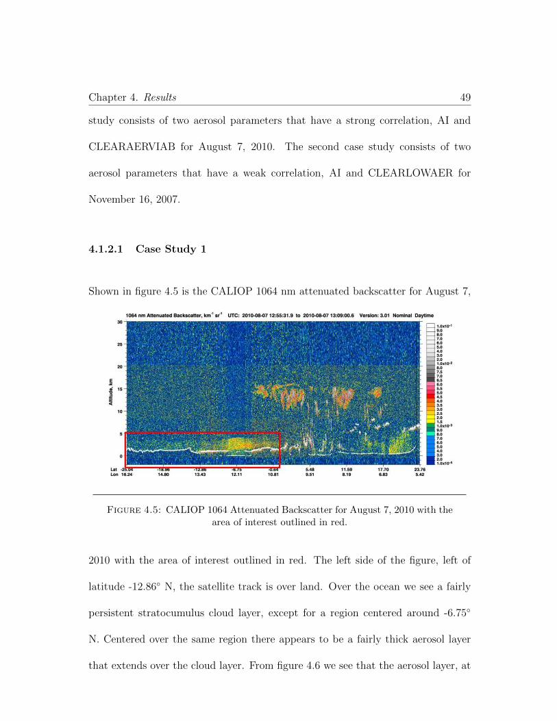
4.1.2.1 Case Study 1 . . . . . . . . . . . . . . . . . . . . . 49
4.1.2.2 Case Study 2 . . . . . . . . . . . . . . . . . . . . . 52
4.2 Cloud Parameters . . . . . . . . . . . . . . . . . . . . . . . . . . . . 54
4.2.1 Cloud Droplet Number Concentration . . . . . . . . . . . . . 55
4.2.2 Effective Radius . . . . . . . . . . . . . . . . . . . . . . . . . 56
4.2.3 Probability of Precipitation . . . . . . . . . . . . . . . . . . 57
4.3 Challenges . . . . . . . . . . . . . . . . . . . . . . . . . . . . . . . . 59
5 Conclusions 64
A Cloud Parameters 68
B Probability of Precipitation 79
Bibliography 81

List of Figures v
List of Figures
1.1 Map of study area outlined in blue. . . . . . . . . . . . . . . . . . . 9
3.1 Monthly average of 1064 nm Clear Sky Vertically Integrated Atten-uated Backscatter. . . . . . . . . . . . . . . . . . . . . . . . . . . . 24
3.2 Monthly average of 1064 nm Vertically Integrated Attenuated Backscat-ter. . . . . . . . . . . . . . . . . . . . . . . . . . . . . . . . . . . . . 25
3.3 Base aerosol layer aerosol subtype (entire dataset). . . . . . . . . . 27
3.4 Base aerosol layer aerosol subtype (rain and cloud). . . . . . . . . . 28
3.5 Monthly average MODIS Aerosol Optical Depth (2007-2010). . . . . 29
3.6 Monthly average MODIS AOD by subtype (2007-2010)(all). . . . . 30
3.7 Monthly average MODIS AOD by subtype (2007-2010)(rain andcloud). . . . . . . . . . . . . . . . . . . . . . . . . . . . . . . . . . . 31
3.8 Monthly average MODIS Aerosol Index (2007). . . . . . . . . . . . 33
3.9 Monthly average aerosol above cloud fraction (2007-2010). . . . . . 35
3.10 Monthly average aerosol touching cloud fraction (2007-2010). . . . . 37
4.1 AI vs. CLEARAERVIAB . . . . . . . . . . . . . . . . . . . . . . . 43
4.2 AI vs. CLEARLOWAER . . . . . . . . . . . . . . . . . . . . . . . . 44
4.3 Cloud, Touch, Top . . . . . . . . . . . . . . . . . . . . . . . . . . . 46
4.4 Rain, Above, Middle . . . . . . . . . . . . . . . . . . . . . . . . . . 47
4.5 CALIOP 1064 nm Backscatter-August 7, 2010 . . . . . . . . . . . . 49
4.6 CALIOP VFM-August 7, 2010 . . . . . . . . . . . . . . . . . . . . . 50
4.7 Map of Aerosol Concentration-August 7, 2010 . . . . . . . . . . . . 51
4.8 CALIOP 1064 nm Backscatter-November 16, 2007 . . . . . . . . . . 52
4.9 CALIOP VFM-Novemver 16, 2007 . . . . . . . . . . . . . . . . . . 53
4.10 Map of Aerosol Concentration-November 16, 2007 . . . . . . . . . . 54
4.11 Cloud Droplet Number Concentration . . . . . . . . . . . . . . . . . 55
4.12 Effective Radius . . . . . . . . . . . . . . . . . . . . . . . . . . . . . 56
4.13 Probability of Precipitation . . . . . . . . . . . . . . . . . . . . . . 57
A.1 CDNC: AI (RAM) . . . . . . . . . . . . . . . . . . . . . . . . . . . 68
A.2 CDNC: AI (RAB) . . . . . . . . . . . . . . . . . . . . . . . . . . . . 68

List of Figures vi
A.3 CDNC: AI (RTT) . . . . . . . . . . . . . . . . . . . . . . . . . . . . 69
A.4 CDNC: AI (RTB) . . . . . . . . . . . . . . . . . . . . . . . . . . . . 69
A.5 CDNC: AI (CTT) . . . . . . . . . . . . . . . . . . . . . . . . . . . . 69
A.6 CDNC: AI (CAM) . . . . . . . . . . . . . . . . . . . . . . . . . . . 69
A.7 CDNC: AI (CAB) . . . . . . . . . . . . . . . . . . . . . . . . . . . . 69
A.8 CDNC: AI (CTM) . . . . . . . . . . . . . . . . . . . . . . . . . . . 69
A.9 CDNC: AOD (RAM) . . . . . . . . . . . . . . . . . . . . . . . . . . 70
A.10 CDNC: AOD (RTT) . . . . . . . . . . . . . . . . . . . . . . . . . . 70
A.11 CDNC: AOD (CAM) . . . . . . . . . . . . . . . . . . . . . . . . . . 70
A.12 CDNC: AOD (CAB) . . . . . . . . . . . . . . . . . . . . . . . . . . 70
A.13 CDNC: AOD (CTM) . . . . . . . . . . . . . . . . . . . . . . . . . . 70
A.14 CDNC: AERVIAB (CAT) . . . . . . . . . . . . . . . . . . . . . . . 70
A.15 CDNC: AERVIAB (CAM) . . . . . . . . . . . . . . . . . . . . . . . 71
A.16 CDNC: AERVIAB (CAB) . . . . . . . . . . . . . . . . . . . . . . . 71
A.17 CDNC: VIAB (RAT) . . . . . . . . . . . . . . . . . . . . . . . . . . 71
A.18 CDNC: VIAB (RAM) . . . . . . . . . . . . . . . . . . . . . . . . . 71
A.19 CDNC: VIAB (RAB) . . . . . . . . . . . . . . . . . . . . . . . . . . 71
A.20 CDNC: VIAB (CAT) . . . . . . . . . . . . . . . . . . . . . . . . . . 71
A.21 CDNC: VIAB (CAM) . . . . . . . . . . . . . . . . . . . . . . . . . 72
A.22 CDNC: VIAB (CAB) . . . . . . . . . . . . . . . . . . . . . . . . . . 72
A.23 CDNC: CLEARAERVIAB (CAM) . . . . . . . . . . . . . . . . . . 72
A.24 CDNC: CLEARAERVIAB (CAB) . . . . . . . . . . . . . . . . . . . 72
A.25 CDNC: CLEARAERVIAB (CTM) . . . . . . . . . . . . . . . . . . 72
A.26 CDNC: CLEARVIAB (CTT) . . . . . . . . . . . . . . . . . . . . . 72
A.27 CDNC: CLEARTOTAER (CAT) . . . . . . . . . . . . . . . . . . . 73
A.28 CDNC: CLEARTOTAER (CAB) . . . . . . . . . . . . . . . . . . . 73
A.29 CDNC: CLEARTOTAER (CTT) . . . . . . . . . . . . . . . . . . . 73
A.30 CDNC: CLEARTOTAER (CTM) . . . . . . . . . . . . . . . . . . . 73
A.31 CDNC: CLEARLOWAER (RAB) . . . . . . . . . . . . . . . . . . . 73
A.32 CDNC: CLEARLOWAER (CTT) . . . . . . . . . . . . . . . . . . . 73
A.33 Eff. Radius: AI (RAT) . . . . . . . . . . . . . . . . . . . . . . . . . 74
A.34 Eff. Radius: AI (RAM) . . . . . . . . . . . . . . . . . . . . . . . . . 74
A.35 Eff. Radius: AI (CAT) . . . . . . . . . . . . . . . . . . . . . . . . . 74
A.36 Eff. Radius: AI (CAM) . . . . . . . . . . . . . . . . . . . . . . . . . 74
A.37 Eff. Radius: AI (CAB) . . . . . . . . . . . . . . . . . . . . . . . . . 75
A.38 Eff. Radius: AOD (RAT) . . . . . . . . . . . . . . . . . . . . . . . 75
A.39 Eff. Radius: AOD (RAM) . . . . . . . . . . . . . . . . . . . . . . . 75
A.40 Eff. Radius: AOD (RAB) . . . . . . . . . . . . . . . . . . . . . . . 75
A.41 Eff. Radius: AOD (CAM) . . . . . . . . . . . . . . . . . . . . . . . 75

List of Figures vii
A.42 Eff. Radius: AOD (CAB) . . . . . . . . . . . . . . . . . . . . . . . 75
A.43 Eff. Radius: AOD (CTM) . . . . . . . . . . . . . . . . . . . . . . . 76
A.44 Eff. Radius: AERVIAB (CAT) . . . . . . . . . . . . . . . . . . . . 76
A.45 Eff. Radius: AERVIAB (CAM) . . . . . . . . . . . . . . . . . . . . 76
A.46 Eff. Radius: AERVIAB (CAB) . . . . . . . . . . . . . . . . . . . . 76
A.47 Eff. Radius: AOD (CTT) . . . . . . . . . . . . . . . . . . . . . . . 76
A.48 Eff. Radius: VIAB (RAT) . . . . . . . . . . . . . . . . . . . . . . . 76
A.49 Eff. Radius: VIAB (RAM) . . . . . . . . . . . . . . . . . . . . . . . 77
A.50 Eff. Radius: VIAB (RAB) . . . . . . . . . . . . . . . . . . . . . . . 77
A.51 Eff. Radius: VIAB (CAT) . . . . . . . . . . . . . . . . . . . . . . . 77
A.52 Eff. Radius: VIAB (CAM) . . . . . . . . . . . . . . . . . . . . . . . 77
A.53 Eff. Radius: VIAB (CAB) . . . . . . . . . . . . . . . . . . . . . . . 77
A.54 Eff. Radius: CLEARAERVIAB (CTM) . . . . . . . . . . . . . . . . 77
A.55 Eff. Radius: CLEARVIAB (RAB) . . . . . . . . . . . . . . . . . . . 78
A.56 Eff. Radius: CLEARVIAB (CTT) . . . . . . . . . . . . . . . . . . . 78
A.57 Eff. Radius: CLEARTOT (RAB) . . . . . . . . . . . . . . . . . . . 78
A.58 Eff. Radius: CLEARTOTAER (CAT) . . . . . . . . . . . . . . . . . 78
A.59 Eff. Radius: CLEARTOTAER (CTM) . . . . . . . . . . . . . . . . 78
A.60 Eff. Radius: CLEARLOWAER (CTT) . . . . . . . . . . . . . . . . 78
B.1 POP: CLEARLOW . . . . . . . . . . . . . . . . . . . . . . . . . . . 79
B.2 POP: AERVIAB . . . . . . . . . . . . . . . . . . . . . . . . . . . . 79
B.3 POP: VIAB . . . . . . . . . . . . . . . . . . . . . . . . . . . . . . . 80
B.4 POP: CLEARTOT . . . . . . . . . . . . . . . . . . . . . . . . . . . 80
B.5 POP: CLEARTOTAER . . . . . . . . . . . . . . . . . . . . . . . . 80
B.6 POP: CLEARVIAB . . . . . . . . . . . . . . . . . . . . . . . . . . . 80

List of Tables viii
List of Tables
2.1 Cloud and aerosol subtyping categories. . . . . . . . . . . . . . . . . 12
3.1 Scene classification requirements. . . . . . . . . . . . . . . . . . . . 17

Chapter 1. Introduction 1
Chapter 1
Introduction
Aerosols play an important role in the radiation and energy budget of Earth as well
as in the hydrologic cycle. Aerosols affect the radiation and energy budget through
the direct aerosol effect, the semi-direct aerosol effect, and two indirect aerosol
effects. The direct aerosol effect is due to the absorptive and scattering properties
of aerosols themselves. Most aerosols are efficient at scattering incoming shortwave
solar radiation; this leads to an increase in the amount of radiation reflected back
to space in a column with a heavy aerosol load. Increasing the amount of incoming
solar radiation that is reflected back to space has a negative (cooling) effect on
the climate. The semi-direct aerosol effect occurs when absorbing aerosols warm
an atmospheric layer and either hinder cloud formation or cause cloud droplets
to evaporate (Ackerman et al. 2000). This might also lead to the suppression of

Chapter 1. Introduction 2
precipitation in the affected region. Until recently, this effect was believed to have
a net warming effect on the planet. However, there is now evidence that the semi-
direct effect may have a net cooling effect on the climate (Kaufman et al. 2005;
Penner et al. 2003).
As described in the Intergovernmental Panel on Climate Change Fourth Assessment
Report (IPCC-4AR), the indirect aerosol effect can be further divided into the first
and second indirect effects (Forster and Ramaswamy 2007). The first indirect effect,
originally proposed by Twomey (1974), is a theory that describes aerosol effects
on radiative forcing due to aerosols altering microphysical cloud properties. The
presence of aerosols in a cloud layer increases the number of cloud condensation
nuclei (CCN). An increase in CCN leads to a greater number of cloud droplets
within a cloud, which will then increase the optical depth of the cloud since an
incoming photon will encounter and be scattered by more particles. This, in turn,
leads to an increase in the albedo of the cloud. It is this increase in the albedo of
the cloud due to the presence of aerosols that is the first indirect aerosol effect.
As described in Twomey (1977) and Albrecht (1989), the second indirect effect
states that the presence of aerosols will increase the liquid water content (LWC)
of a cloud through the suppression of drizzle formation. Through an increase in
LWC, aerosols will likely increase cloud top height and cloud lifetime (Forster and
Ramaswamy 2007). The mechanism behind the suppression of rain relates to the
collision-coalescence process. If the amount of liquid water is held constant within

Chapter 1. Introduction 3
a given cloud layer, cloud droplets in a polluted air mass will be smaller than in
a clean air mass. This reduces the efficiency of the collision-coalescence process
within clouds because the efficiency of this process largely depends on the radius of
the largest cloud drops. Jonas (1996) explains that the initial formation of drizzle
requires coalescence of cloud droplets since growth by condensation is too slow of
a process. In that study the critical effective radius was roughly 20 µm. In a more
recent study, Rosenfeld et al. (2012) found that this critical effective radius is 12-14
µm. The absence of large cloud drops in polluted air masses leads to a reduced
efficiency in the drizzle formation process. This leads to a decrease, and in extreme
cases, complete suppression, of the precipitation in a given cloud. Since the cloud
is no longer precipitating efficiently, the cloud lifetime will increase. The increased
liquid water content and increased cloud lifetime allow for increased latent heat
release within the cloud. This makes the cloud more buoyant, increasing the cloud
top height (Kaufman et al. 2005; Pawlowska and Brenguier 2003).
Bennartz (2007) found that maximum cloud droplet number concentration (CDNC)
values are found over the continents and minimum CDNC values are found out over
the open ocean. An increase in CDNC may also lead to suppression of precipitation
as seen in boundary layer clouds when moving from the open ocean towards the
coastline. An increase in CDNC is the result of a gradient in aerosols where aerosol
concentration increases closer to lind compared to open ocean. Thus far, the only
global evidence of the second indirect aerosol effect has come from modeling studies

Chapter 1. Introduction 4
where the evidence points to the suppression of precipitation in areas of high aerosol
loading (e.g. Jacobson et al. 2007; Jiang et al. 2002; Lu and Seinfeld 2005).
From a global study involving satellite datasets and a global transport model,
L’Ecuyer et al. (2009) found a more complex relationship between aerosols and
precipitation suppression. First, if the aerosols were mostly made up of sulfate
particles, then precipitation suppression did indeed occur. However, if the aerosols
had a larger concentration of sea salts, then the opposite effect was seen as precip-
itation was enhanced because sea salts are typically larger than sulfate particles.
As a result, sea salts can provide a source for embryonic raindrops, accelerating the
precipitation process and decreasing cloud lifetime as a consequence. Therefore,
the effect aerosols have on precipitation is not only a factor of aerosol loading but
of the composition of the aerosols as well. If sulfates are more abundant, precip-
itation may be suppressed, and if sea salts are more abundant precipitation may
be enhanced. Warm clouds (clouds from this point on) with low LWP values will
not precipitate in most instances regardless of aerosol load while clouds with high
LWP values would need exceptionally large CDNC values to suppress precipitation.
However, clouds with moderate (250-375 gm-2) liquid water path (LWP) values are
most susceptible to changes in aerosol loading. It was also noted that there is
evidence of a reduction in drizzle drop concentration within marine stratocumulus
cloud decks in certain places. Out in the open ocean, the only process that could
account for a reduction in drizzle in such a specific area is the increase in aerosol

Chapter 1. Introduction 5
load as a result of emissions from ships.
From an in situ field study, Pawlowska et al. (1999) also found that precipitation
efficiency is more likely to be higher in a clean marine air mass than in a polluted air
mass. In addition, Pawlowska and Brenguier (2003) found that drizzle is reduced at
a rate proportional to H3/N where H is the geometric thickness of the cloud and N
is CDNC. Geometric thickness is a measure of how thick a cloud would be if it were
completely homogeneous. In shallow stratiform clouds, variations in CDNC are
more important in determining precipitation efficiency than variations in geometric
thickness because these clouds are really shallow regardless of CDNC concentration.
Bennartz (2007) utilized this relationship to define a drizzle threshold. Areas where
drizzle was likely to be occurring was defined to be where H3
N> 0.4. Depending on
the relationship used, this ratio corresponds to drizzle rates between 0.5 mm/day
and 2.5 mm/day.
Other studies have defined a drizzle threshold using another satellite-derived pa-
rameter, effective radius. Painemal and Zuidema (2011) concluded that drizzle
could be identified from MODIS effective radius retrievals. Using the standard 2.1
µm wavelength effective radius retrieval, a threshold for precipitation onset was
found to be when the effective radius is around 12 µm. A 12 µm threshold cor-
responds to radar reflectivity values between -19 dBz and -15 dBz. These values
are consistent with drizzle onset found in multiple studies (e.g. Chin et al. 2000;
Frisch et al. 1995; Liu et al. 2008; Wang and Geerts 2003). The drizzle threshold
Chapter 1. Introduction 6
found by Frisch et al. (1995) utilized a Kα-band radar (8.66 mm wavelength) while
Chin et al. (2000) and Wang and Geerts (2003) utilized a W-band radar (3 mm).
The direct aerosol effect, semi-direct aerosol effect, and two indirect aerosol effects
are important areas of climate research because the single largest source of un-
certainty when evaluating climate forcing is aerosols effects. The uncertainty in
the cloud albedo effect is 1.5 W/m2. The cloud albedo effect is also known as the
first indirect effect and is described above. The next largest uncertainty is only
0.8 W/m2 from the direct aerosol effect. These are significant because the largest
uncertainty from a forcing not related to aerosols is only 0.4 W/m2 for the change
in surface albedo due to land use and changes in tropospheric ozone concentration
(Forster and Ramaswamy 2007).
Multiple studies (Kaufman et al. 2005; L’Ecuyer et al. 2009; Rosenfeld 2000) have
shown that the various aerosol effects described above have a noticeable impact
on cloud formation and precipitation efficiency. Consistent with the indirect ef-
fects, these studies have found that an increase in aerosol concentration leads to
an increase in CDNC and a decrease in effective radius. The decrease in effective
radius then leads to precipitation suppression, as the cloud drops are not large
enough for the initiation of the collision-coalescence process. Furthermore, Kauf-
man et al. (2005) found that not only does an increase in aerosol concentration lead
to precipitation suppression, but also to a systematic increase in cloud cover. The
increased cloud cover is the result of increased cloud condensation nuclei in pristine

Chapter 1. Introduction 7
marine air where cloud formation would be extremely difficult. Increased aerosol
concentration led to more cloud formation closer to the African coast in a region
characterized by biomass burning. In another study, Wu et al. (2013) found that
by acting as CCN, aerosols can decrease cloud droplet size and lower precipitation
efficiency within the monsoon rains in East Asia. Bennartz et al. (2011) found that
pollution from China increases CDNC and suppresses rain over the East China
Sea.
Another study, Costantino and Breon (2013), found that the cloud droplet radius-
cloud optical thickness relationship is positive for non-precipitating clouds and
negative for precipitating clouds. In addition, for large aerosol index values, the
cloud droplet radius is 3-5 µm smaller than in clean conditions. Interestingly, for
the clouds they studied, they found that thin liquid clouds have smaller liquid
water path values in the presence of polluted atmospheric layers while thick liquid
clouds have larger liquid water paths. With these results, the authors concluded
that the impact of aerosols on cloud microphysics is strong.
Using the Tropical Rainfall Measuring Mission (TRMM) satellite, Rosenfeld (2000)
found clear evidence that smoke from biomass burning events suppresses precipi-
tation. Furthermore, “pollution tracks” were found to also have reduced precipi-
tation. “Pollution tracks” are defined to be tracks of pollution clearly evident in
satellite imagery. Most pollution tracks are located downwind of point sources of
pollution, such as power plants and major population centers. Within a given air

Chapter 1. Introduction 8
mass, clouds in the pollution tracks had reduced or suppressed precipitation, while
clouds outside of the pollution track did not experience reduced or suppressed
precipitation. Various measurements taken from TRMM indicate that the lack
of precipitation within pollution tracks was not the result of an air mass change
or any other meteorological process. The precipitation suppression within pollu-
tion tracks is consistent with the precipitation suppression seen within ship tracks.
Both pollution and ship tracks provide valuable evidence supporting the hypothesis
that increased aerosol concentrations lead to precipitation suppression through the
processes described by the different aerosol effects.
The objective of this study is two-fold. First, the primary objective is to identify
observational challenges in assessing the aerosol indirect and semi-direct effect.
A secondary objective is to use observations to further test the hypothesis that
aerosol concentration leads to precipitation suppression by focusing on precipitation
efficiency in stratiform warm clouds in the South Atlantic Ocean off the west coast
of Africa.
The study region is defined to be between 5◦S and 25◦S and 10◦W and 15◦E (Figure
1.1). This region is an ideal region to study the effects of aerosols on precipitation
efficiency due to large but periodic sources of aerosols in this region due to biomass
burning. The biomass burning season in Africa’s southern half ranges from May
through October, with a peak in the area of study occurring in the latter half of the
season, or about July through October. As the season progresses, shrub land and

Chapter 1. Introduction 9
-45 -30 -15 0 15 30 45
-40
-30
-20
-10
0
10
20
30
40
Figure 1.1: Map of study area outlined in blue.
grassland become the dominant fuel types (Roberts et al. 2009). The presence of
biomass burning leads to the transport of large amounts of aerosols into the South
Atlantic Ocean as a consequence of the prevailing easterly winds in the subtropics.
Aerosols from biomass burning are usually trapped below 3km, the height of the
inversion that typically is found in this part of the tropics and subtropics. As a
result, smoke particles will be able to act as CCN in warm clouds (Crutzen and
Andreae 1990).

Chapter 2. Instruments and Datasets 10
Chapter 2
Instruments and Datasets
2.1 CALIOP
The Cloud-Aerosol LIdar with Orthogonal Polarization (CALIOP) instrument is a
dual-wavelength polarization-sensitive lidar operating aboard the Cloud-Aerosol Li-
dar and Infrared Pathfinder Satellite Observations (CALIPSO) satellite. CALIPSO
flies as a part of the NASA A-TRAIN constellation of satellites, which is in sun
synchronous orbit with a 1:30pm local time equator crossing. CALIOP operates at
532 nm and 1064 nm at a high resolution of 30-60 m vertically and 333 m horizon-
tally. CALIOP is sensitive to the presence of aerosols as well as cloud top height
as a result of the high resolution and wavelengths chosen. The 532 nm channel
operates with two orthogonally polarized components, perpendicular and parallel.

Chapter 2. Instruments and Datasets 11
The dual-polarization data allows for a more robust determination of many aerosol
variables, including aerosol type, orientation, and shape. In addition to the attenu-
ated backscatter and vertical feature mask defined below, cloud top height (CTH)
is also retrieved from CALIOP.
2.1.1 Attenuated Backscatter
The 1064 nm channel attenuated backscatter product (units of km-1 sr-1) is a part
of the LIDAR Level 1 Data products. The 1064 nm channel attenuated backscatter
is used instead of the 532 nm channel as there is less noise in this band since it is
further from the wavelength of maximum emission of the sun (482 nm assuming a
temperature of 6000 K). The 1064 nm attenuated backscatter has a nominal range
of 0.0 to 2.0 km-1 sr-1 and is reported at 583 levels in the vertical profile.
2.1.2 Vertical Feature Mask
The vertical feature mask is a LIDAR Level 2 Data product. The vertical feature
mask classifies every data point, both vertically and horizontally, into one of seven
classification types: clear air, cloud, aerosol, stratospheric layer, surface, subsur-
face, and totally attenuated (Powell and Vaughan 2013). Every point identified as
either cloud or aerosol is then further subtyped. Clouds can be subtyped into four
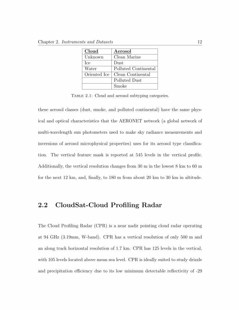
categories and aerosol can be subtyped into six categories (Table 2.1). Three of
Chapter 2. Instruments and Datasets 12
Cloud AerosolUnknown Clean MarineIce DustWater Polluted ContinentalOriented Ice Clean Continental
Polluted DustSmoke
Table 2.1: Cloud and aerosol subtyping categories.
these aerosol classes (dust, smoke, and polluted continental) have the same phys-
ical and optical characteristics that the AERONET network (a global network of
multi-wavelength sun photometers used to make sky radiance measurements and
inversions of aerosol microphysical properties) uses for its aerosol type classifica-
tion. The vertical feature mask is reported at 545 levels in the vertical profile.
Additionally, the vertical resolution changes from 30 m in the lowest 8 km to 60 m
for the next 12 km, and, finally, to 180 m from about 20 km to 30 km in altitude.
2.2 CloudSat-Cloud Profiling Radar
The Cloud Profiling Radar (CPR) is a near nadir pointing cloud radar operating
at 94 GHz (3.19mm, W-band). CPR has a vertical resolution of only 500 m and
an along track horizontal resolution of 1.7 km. CPR has 125 levels in the vertical,
with 105 levels located above mean sea level. CPR is ideally suited to study drizzle
and precipitation efficiency due to its low minimum detectable reflectivity of -29
Chapter 2. Instruments and Datasets 13
dBZe. CPR currently flies on the CloudSat satellite, which was launched in 2006.
CloudSat flies as a part of NASA’s A-TRAIN.
2.2.1 Level 2 Data
The reflectivity profile from CPR is used to help monitor the precipitation efficiency
within the stratocumulus clouds in this region. However, the light drizzle that this
study focuses on cannot be reliably detected below roughly 1 km because the
outgoing radar pulse not a perfect square wave, thereby increasing the surface
clutter in the data up to roughly 1 km above the surface (Marchand et al. 2008).
2.2.2 2C-PRECIP-COLUMN
The 2C-PRECIP-COLUMN product estimates the occurrence of precipitation and
its intensity at the surface. The precipitation flag indicates the presence of pre-
cipitation using CPR reflectivity as a basis for this determination. There are four
possible values for this flag: 0-no precipitation detected, 1-rain possible, 2-rain
probable, and 3-rain certain. Roughly speaking, the rain possible flag corresponds
to reflectivity values greater than -15 dBZ, the rain probable flag corresponds to
reflectivity values greater than -7 dBZ, and the rain certain flag corresponds to
Chapter 2. Instruments and Datasets 14
reflectivity values greater than 0 dBZ. This study utilizes the status flag in con-
junction with the precipitation flag. The status flag reports if the retrieval suc-
cessfully determined the incidence and intensity of precipitation, just the incidence
of precipitation, or if there was an error in the retrieval. The following is a list of
reasons an error could have occurred: reflectivity profile bad, gaseous attenuation
missing, sea surface temperature missing, surface wind speed missing, σ0 (surface
attenuated backscatter cross section) could not be determined, cloud base could
not be determined, near surface reflectivity missing, or freezing level could not be
determined.
2.3 MODIS
The MODerate resolution Imaging Spectroradiometer (MODIS) is an imaging in-
strument with 36 spectral bands covering the entire solar and terrestrial infrared
spectral range. MODIS has roughly a 1 km spatial resolution, but this is dependent
on which band is used. MODIS flies aboard two Earth Observing System satellites,
Aqua and Terra. For this study, the MODIS instrument aboard Aqua was used.
As with CloudSat and CALIPSO, Aqua is flown in NASA’s A-TRAIN.

Chapter 2. Instruments and Datasets 15
2.3.1 Cloud Parameters
This study utilizes the Level 2 MODIS cloud products subset along the CloudSat
field of view track. This dataset contains cloud optical and microphysical prop-
erties including: cloud top temperature (CTT), cloud top pressure (CTP), cloud
optical depth (COD), and effective radius. These products are derived from varying
combinations of the 36 spectral bands that make up MODIS.
2.3.2 Level-3 Daily Global Gridded Data
Aerosol optical depth from the MODIS Level 3 daily global gridded data at 1◦x1◦
resolution is used as an alternative method to calculate column averaged atmo-
spheric aerosol concentration. This product is derived from the Level 2 atmo-
sphere products. The statistics for each science parameter are then aggregated
onto a 1◦x1◦ equal-angle global grid.

Chapter 3. Evaluation Methods 16
Chapter 3
Evaluation Methods
3.1 Scene Classification
The four-year (2007-2010) dataset used in this study is divided into three categories-
rainy, cloudy, and clear-in order to isolate the effects of aerosols on precipitation
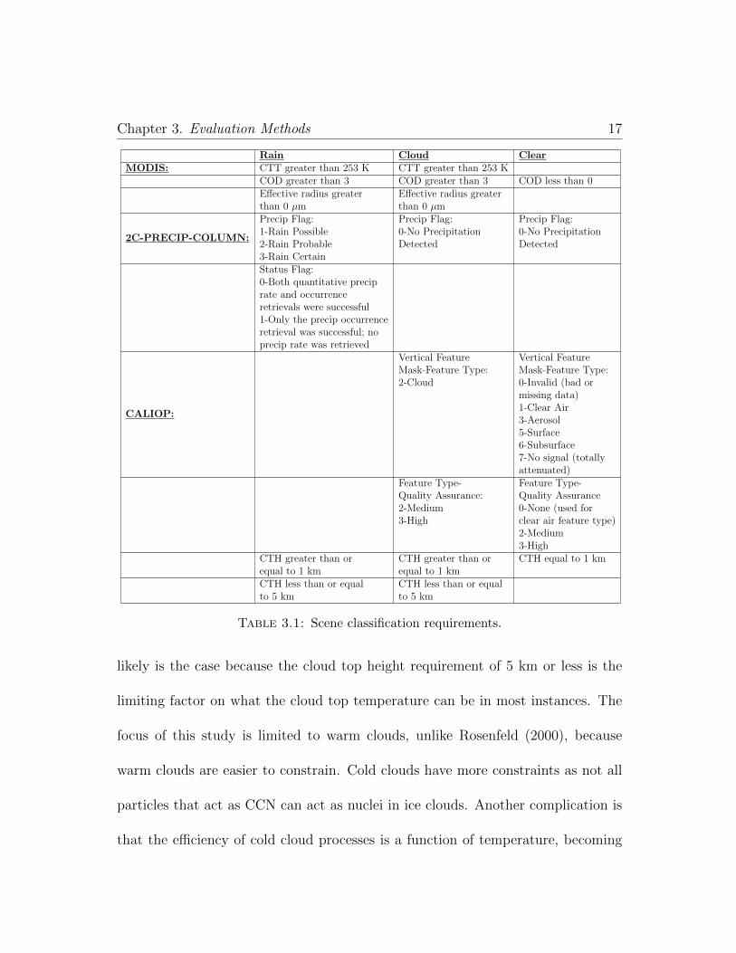
efficiency. The scene classification requirements can be found in Table 3.1. Some
requirements, such as cloud top height greater than or equal to 0 km in the clear
classification, are used to ensure that the data used are valid for a column. The
cloud top temperature requirement of 253 K to allow for supercooled water to be
present in the cloud. Increasing the cloud top temperature to 273 K makes only
a minor difference in the number of columns identified as there are only 287 rainy
or cloudy columns that have a cloud top temperature below 273 K. This most
Chapter 3. Evaluation Methods 17
Rain Cloud ClearMODIS: CTT greater than 253 K CTT greater than 253 K
COD greater than 3 COD greater than 3 COD less than 0Effective radius greater Effective radius greaterthan 0 µm than 0 µm
2C-PRECIP-COLUMN:
Precip Flag: Precip Flag: Precip Flag:1-Rain Possible 0-No Precipitation 0-No Precipitation2-Rain Probable Detected Detected3-Rain CertainStatus Flag:0-Both quantitative preciprate and occurrenceretrievals were successful1-Only the precip occurrenceretrieval was successful; noprecip rate was retrieved
CALIOP:
Vertical Feature Vertical FeatureMask-Feature Type: Mask-Feature Type:2-Cloud 0-Invalid (bad or
missing data)1-Clear Air3-Aerosol5-Surface6-Subsurface7-No signal (totallyattenuated)
Feature Type- Feature Type-Quality Assurance: Quality Assurance2-Medium 0-None (used for3-High clear air feature type)
2-Medium3-High
CTH greater than or CTH greater than or CTH equal to 1 kmequal to 1 km equal to 1 kmCTH less than or equal CTH less than or equalto 5 km to 5 km
Table 3.1: Scene classification requirements.
likely is the case because the cloud top height requirement of 5 km or less is the
limiting factor on what the cloud top temperature can be in most instances. The
focus of this study is limited to warm clouds, unlike Rosenfeld (2000), because
warm clouds are easier to constrain. Cold clouds have more constraints as not all
particles that act as CCN can act as nuclei in ice clouds. Another complication is
that the efficiency of cold cloud processes is a function of temperature, becoming
Chapter 3. Evaluation Methods 18
more efficient as the temperature drops. Peak efficiency is between -10◦ and -
20◦C (Cotton et al. 1986). Cold clouds also have interfering processes that make
them harder to analyze. Using the classification scheme just described, our dataset
has 31,692 rainy columns, 162,950 cloudy columns, and 262,115 clear columns.
The data is then further classified by the presence of an aerosol layer above cloud
top, as identified by the CALIOP VFM. Once the columns with aerosol layers
are identified, the difference between cloud top height and aerosol base height is
determined. If this difference in height is less than 250 m, the column is identified
as having an aerosol layer touching the cloud. Otherwise, the column is identified as
having an aerosol layer above the cloud. Out of the 31,692 rainy columns identified,
8,067 columns have an aerosol layer, of which 669 are touching and 7,398 are above
the cloud. Out of the 162,950 cloudy columns, 45,930 have an aerosol layer above
the cloud with 8,855 columns having an aerosol layer touching and 40,075 columns
having an aerosol layer above the cloud. Out of the 262,115 clear columns, 30,884
have an aerosol layer in the column.

Chapter 3. Evaluation Methods 19
3.2 Aerosol Concentration
3.2.1 Vertically Integrated Attenuated Backcatter
3.2.1.1 Methods
As a proxy for aerosol optical depth, the 1064 nm channel attenuated backscatter
and the vertical feature mask are used to measure aerosol concentration within an
atmospheric column. First, the vertical feature mask is used to locate aerosol layers
that are above cloud top or above 1 km in the absence of clouds. Once the aerosol
layers are identified in the column, the 1064 nm attenuated backscatter is used in
a variety of ways to calculate aerosol concentration. The eight calculations that
will be discussed in this section are: clear sky integrated boundary layer backscat-
ter (total), CLEARTOT ; clear sky integraged elevated boundary layer backscatter
(elevated), CLEARV IAB; clear sky integrated surface boundary layer backscatter
(low), CLEARLOW ; clear sky integrated aerosol boundary layer backscatter (total
aerosol), CLEARTOTAER; clear sky integrated elevated aerosol boundary layer
backscatter (elevated aerosol), CLEARAERV IAB; clear sky integrated surface
aerosol boundary layer backscatter (low aerosol), CLEARLOWAER; integrated
elevated boundary layer backscatter (rain/cloud total), V IAB; and integrated el-
evated aerosol boundary layer backscatter (rain/cloud aerosol), AERV IAB. The
last two aerosol parameters will have a slightly different interpretation than the first
Chapter 3. Evaluation Methods 20
six aerosol parameters. The first aerosol parameter, clear sky integrated boundary
layer backscatter, is calculated according to the following equation:
CLEARTOT =
z=5000m∫z=0m
σbdz, (3.1)
where σb is the attenuated backscatter at 1064 nm and CLEARTOT has units of
sr−1. The second aerosol parameter, clear sky integrated elevated boundary layer
backscatter, is calculated as follows:
CLEARV IAB =
z=5000m∫z=1000m
σbdz. (3.2)
The third aerosol parameter, clear sky integrated surface boundary layer backscat-
ter, is calculated according to the following equation:
CLEARLOW =
z=1000m∫z=0m
σbdz. (3.3)
The fourth aerosol parameter, clear sky integrated aerosol boundary layer backscat-
ter, is calculated as follows:
CLEARTOTAER =
z=5000m∫z=0m
σb(V FMFT = 3)dz, (3.4)
where V FMFT = 3 is the vertical feature mask-feature type that corresponds to
aerosol. The fifth aerosol parameter, clear sky integrated elevated aerosol boundary

Chapter 3. Evaluation Methods 21
layer backscatter, is calculated according to the following equation:
CLEARAERV IAB =
z=5000m∫z=1000m
σb(V FMFT = 3)dz. (3.5)
The sixth aerosol parameter, clear sky integrated surface aerosol boundary layer
backscatter, is calculated as follows:
CLEARLOWAER =
z=1000m∫z=0m
σb(V FMFT = 3)dz. (3.6)
The first three aerosol parameters integrate through all layers, while the last three
parameters only integrate through layers identified as aerosol by the vertical feature
mask. The clear sky integrated boundary layer backscatter and clear sky integrated
aerosol boundary layer backscatter integrate from 5000m to the surface. The in-
tegration begins at 5000 m because the atmosphere above this level should not
influence the low-level stratocumulus clouds that are the focus of this study. The
clear sky integrated elevated boundary layer backscatter and clear sky integrated
elevated aerosol boundary layer backscatter integrate between 5000 m and 1000 m.
Sea salt should influence these two parameters less than the first two parameters
described. This is a useful distinction, as the focus of this study is on biomass
burning aerosols being transported over the stratocumulus clouds, not the sea salt
aerosols that are always present. The last two parameters, clear sky integrated

Chapter 3. Evaluation Methods 22
surface boundary layer backscatter and clear sky integrated surface aerosol bound-
ary layer backscatter, are calculated only through the lowest 1000 m. This, again,
is done to try and isolate the effects of sea salt from that of the biomass burning
aerosols.
These six aerosol parameters are only calculated in columns identified as clear sky,
according to the classification scheme previously described. The parameters are
then separated into 1◦x1◦ bins and averaged. The average aerosol concentration
is calculated daily. Once the data is binned, it is co-located with the rainy and
cloudy pixels. Each rainy and cloudy pixel is assigned an aerosol concentration
based on the 1◦x1◦ bin in which it was located. This aids in assessing the relation-
ship between aerosol concentration and various cloud macro- and micro- physical
properties.
The final two aerosol parameters, integrated elevated boundary layer backscat-
ter and integrated elevated aerosol boundary layer backscatter, are calculated as
follows:
V IAB =
z=5000m∫z=zbot
σbdz, and (3.7)
AERV IAB =
z=5000m∫z=zbot
σb(V FMFT = 3)dz, (3.8)
where zbot = 1000 m in the absence of clouds or if the cloud top height is below
1000 m, or zbot = CTH+90 m in the presence of clouds. The purpose of integrating

Chapter 3. Evaluation Methods 23
to 90 m above cloud top is to avoid integrating through the cloud layer, as this
would drastically increase the vertically integrated attenuated backscatter for that
column. Furthermore, given the wavelengths that CALIOP operates at, the signal
becomes rapidly attenuated in the presence of clouds. Contrary to the first six
aerosol parameters, these last two parameters are only calculated for columns where
a cloud (rain or cloud column) is detected. As a consequence, these two parameters
do not need to be binned, averaged, and co-located in order to be matched up with
cloud properties. Additionally, these last two aerosol parameters can no longer be
compared to the MODIS aerosol parameters as they are no longer looking at the
same scene. This will be discussed in the following sections.
3.2.1.2 Results
Figure 3.1 shows the results of the six clear sky calculations as a monthly average
for the combined dataset of rain and cloud column identification. The magnitude
of each calculation relative to the other calculations is consistent with expectations;
total is greater than elevated which is greater than low, and total aerosol is greater
than both elevated aerosol and low aerosol. The only relative magnitude that
may be somewhat surprising is that the low aerosol is greater than the elevated
aerosol for January-March and October-December. This would lead one to believe
that outside the biomass burning season there is little aerosol transported above
the stratocumulus cloud layer. Interestingly, total appears to have three maxima,

Chapter 3. Evaluation Methods 24
Mean VIAB (Clear Colocated)(2007-2010)
Jan Feb Mar Apr May Jun Jul Aug Sep Oct Nov DecMonths
0.00
0.02
0.04
0.06
0.08V
ertic
ally
Inte
grat
ed A
ttenu
ated
Bac
ksca
tter
[sr-1
]
TotalTotal AerosolElevatedElevated AerosolLowLow Aerosol
Figure 3.1: Monthly average of the six 1064 nm Clear Sky Vertically IntegratedAttenuated Backscatter (sr−1)(VIAB) calculations for 2007-2010. Total is theintegration from the surface to 5 km, Total Aerosol is the integration from thesurface to 5 km integrating only through aerosol layers, Elevated is the integra-tion from 1 km to 5 km, Elevated Aerosol is the integration from 1 km to 5 kmintegrating only through aerosol layers, Low is the integration from the surfaceto 1 km, and Low Aerosol is the integration from the surface to 1 km integrating
only through aerosol layers.
April, July, and October. All three months are somewhat surprising. While July
and October are within the biomass burning season, they are at the beginning
and end of the season, not when one would expect the season to be strongest.
The April peak in total appears to be the result of a peak in the elevated curve
during the same month. Elevated appears to be the dominant contributor to the
total concentration. The low concentration does account for the peak in the total
concentration in July and October, however. It is unclear why there is a peak in low

Chapter 3. Evaluation Methods 25
level backscatter during these months. Total aerosol appears to follow the trend of
low aerosol outside of the biomass burning season and elevated aerosol during the
biomass burning season, especially August and September. Therefore, it appears
that more aerosol is being transported into the region during the biomass burning
season. Interestingly, however, the biggest peak in total aerosol occurs in July,
when both low aerosol and elevated aerosol have a maximum. Total aerosol also
does not appear to make up a large portion of the total backscatter.
Mean VIAB (Rain/Cloud)(2007-2010)
Jan Feb Mar Apr May Jun Jul Aug Sep Oct Nov DecMonths
0.00
0.01
0.02
0.03
0.04
Vert
ically
Inte
gra
ted A
ttenuate
d B
ackscatter
[sr-1
]
TotalAerosol
Figure 3.2: Monthly average of the two 1064 nm Vertically Integrated Atten-uated Backscatter (sr−1)(VIAB) calculations for 2007-2010. Total is the inte-gration from z = zbot to 5 km, Aerosol is the integration from z = zbot to 5 km
integrating only through aerosol layers.
Figure 3.2 shows the result of the two aerosol calculations that were calculated from
Chapter 3. Evaluation Methods 26
the rainy and cloudy columns directly. Again, we see that the total is greater than
aerosol. We see that the total from this figure is smaller in magnitude than the
elevated from figure 3.1 and that aerosol is similar to elevated aerosol, especially
during the biomass burning season. Unlike elevated and elevated aerosol, though,
total and aerosol from the rain/cloud identification do experience a maximum dur-
ing the biomass burning season, as would be expected.
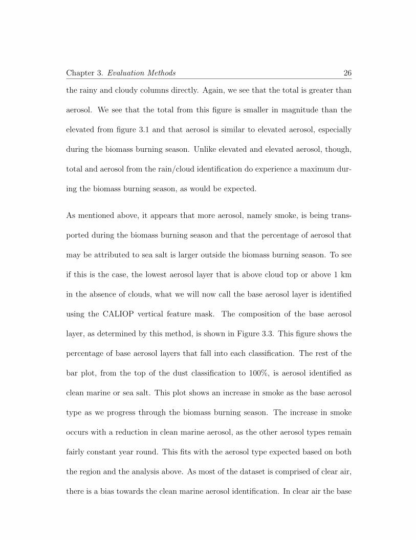
As mentioned above, it appears that more aerosol, namely smoke, is being trans-
ported during the biomass burning season and that the percentage of aerosol that
may be attributed to sea salt is larger outside the biomass burning season. To see
if this is the case, the lowest aerosol layer that is above cloud top or above 1 km
in the absence of clouds, what we will now call the base aerosol layer is identified
using the CALIOP vertical feature mask. The composition of the base aerosol
layer, as determined by this method, is shown in Figure 3.3. This figure shows the
percentage of base aerosol layers that fall into each classification. The rest of the
bar plot, from the top of the dust classification to 100%, is aerosol identified as
clean marine or sea salt. This plot shows an increase in smoke as the base aerosol
type as we progress through the biomass burning season. The increase in smoke
occurs with a reduction in clean marine aerosol, as the other aerosol types remain
fairly constant year round. This fits with the aerosol type expected based on both
the region and the analysis above. As most of the dataset is comprised of clear air,
there is a bias towards the clean marine aerosol identification. In clear air the base
Chapter 3. Evaluation Methods 27
CALIOP VFM-Aerosol Subtype (2007-2010)
Month
0
20
40
60
80
100
Per
cent
age
of M
onth
ly T
otal
[%]
CALIOP VFM-Aerosol Subtype (2007-2010)
Month
0
20
40
60
80
100
Per
cent
age
of M
onth
ly T
otal
[%]
Jan Feb Mar Apr May Jun Jul Aug Sep Oct Nov Dec
SmokePolluted DustClean ContinentalPolluted ContinentalDust
Figure 3.3: Base aerosol layer aerosol subtype by percentage of total per monthfor the entire dataset. From the top of the dust bar to 100% is clean marine
aerosol.
aerosol layer is most likely at the 1 km lower threshold. At this level, we would
expect an abundance of clean marine aerosol when out over the ocean. In order
to reduce the bias towards clean marine aerosol, the same plot was created from
the combined dataset of the rain and cloud column identification (Figure 3.4). In
this figure the increase in smoke during the biomass burning season is even more
evident. The increase in smoke appears to be at the expense of both clean marine
aerosol and dust. As another check to see if the signal in the vertically integrated
attenuated backscatter calculation is correct, it is then compared with the MODIS
derived aerosol optical depth.

Chapter 3. Evaluation Methods 28
CALIOP VFM-Aerosol Subtype (2007-2010)
Month
0
20
40
60
80
100
Per
cent
age
of M
onth
ly T
otal
[%]
CALIOP VFM-Aerosol Subtype (2007-2010)
Month
0
20
40
60
80
100
Per
cent
age
of M
onth
ly T
otal
[%]
Jan Feb Mar Apr May Jun Jul Aug Sep Oct Nov Dec
No ClearSmokePolluted DustClean ContinentalPolluted ContinentalDust
Figure 3.4: Base aerosol layer aerosol subtype by percentage of total per monthfor rain and cloud columns only. From the top of the dust bar to 100% is clean
marine aerosol.
3.2.2 MODIS Aerosol Optical Depth
In order to use the MODIS Aerosol Optical Depth data, it first has to be co-
located with all columns identified as either rainy or cloudy. Once this is done
the monthly average aerosol optical depth can be calculated (Figure 3.5). It is
important to note that a one-to-one comparison cannot be done between AOD
and the other eight aerosol metrics as the units are not consistent between the
CALIOP vertically integrated attenuated backscatter (sr−1) and MODIS aerosol
optical depth (none). With this in mind, the agreement in shape between AOD and

Chapter 3. Evaluation Methods 29
Mean Colocated MODIS AOD (2007-2010)
Jan Feb Mar Apr May Jun Jul Aug Sep Oct Nov DecMonths
0.0
0.5
1.0
1.5
2.0
2.5M
OD
IS A
ero
sol O
ptical D
epth
[none]
Figure 3.5: Monthly average 1◦x1◦ MODIS Aerosol Optical Depth co-locatedwith all rainy and cloudy columns in the dataset for 2007-2010.
the six clear sky aerosol metrics looks somewhat troublesome (Figure 3.1). MODIS
AOD data shows a peak in aerosol concentration in August and September, much
like rain/cloud total and rain/cloud aerosol, and elevated aerosol. With that being
said, these three CALIOP aerosol metrics are three that MODIS AOD should
correlate with the best. However, we would think that total and total aerosol
would look more like MODIS AOD than they do. This is mostly a consequence of
these two calculations having peaks in April and a minimum in September that the
other aerosol metrics do not have. Since MODIS measures total column aerosol it
makes sense that MODIS AOD would not agree with low and low aerosol as these

Chapter 3. Evaluation Methods 30
two calculations ignore most of the atmospheric column.
Avg Monthly AOD by Base Aerosol (2007-2010)
Month
0.0
0.1
0.2
0.3
Aero
sol O
ptical D
epth
[none]
Avg Monthly AOD by Base Aerosol (2007-2010)
Month
0.0
0.1
0.2
0.3
Aero
sol O
ptical D
epth
[none]
Jan Feb Mar Apr May Jun Jul Aug Sep Oct Nov Dec
Clean MarineSmokePolluted DustClean ContinentalPolluted ContinentalDust
Figure 3.6: Monthly average MODIS AOD by base aerosol subtype for theentire dataset during the time period 2007-2010.
Given the discussion thus far, we would expect that the sharp increase in AOD
during August and September would be the result of biomass burning and that
most of the increase in AOD would be from smoke. To determine if this is the case,
a similar method to the one used to determine the base aerosol layer is employed.
The difference, however, is that in this case there is an extra step. Once the base
aerosol layer is identified, the AOD associated with that column is assigned to that
aerosol subtype. The average AOD associated with each aerosol subtype is plotted
by month in figure 3.6. As we can see, the increase in MODIS AOD is a result of

Chapter 3. Evaluation Methods 31
an increase in smoke as the base aerosol subtype. This confirms that the increase
in AOD is the result of the biomass burning season. As was the case with the base
aerosol subtype, this figure may be biased toward clean marine as a majority of
the dataset consists of clear columns. Monthly average MODIS AOD by subtype
without the clear columns is shown in figure 3.7. The biggest difference is that
Avg Monthly AOD by Base Aerosol (2007-2010)
Month
0.0
0.1
0.2
0.3
Aer
osol
Opt
ical
Dep
th [n
one]
Avg Monthly AOD by Base Aerosol (2007-2010)
Month
0.0
0.1
0.2
0.3
Aer
osol
Opt
ical
Dep
th [n
one]
Jan Feb Mar Apr May Jun Jul Aug Sep Oct Nov Dec
No ClearClean MarineSmokePolluted DustClean ContinentalPolluted ContinentalDust
Figure 3.7: Monthly average MODIS AOD by base aerosol subtype for rainand cloud columns only during the time period 2007-2010.
the increase in smoke during the biomass burning season is even more evident in
this case. The increase in average AOD is more complicated to explain as MODIS
AOD is only calculated under clear sky conditions.

Chapter 3. Evaluation Methods 32
3.2.3 MODIS Aerosol Index
Before looking at the monthly average of MODIS Aerosol Index (AI), it is worth-
while to define what MODIS AI is. MODIS AI is similar to MODIS aerosol optical
depth but is more sensitive to fine mode aerosols. This is because AI is the product
of the AOD and angstrom exponent, AI = AOD ∗AE. The angstrom exponent is
used to describe the dependence of aerosol optical depth on wavelength. AI, there-
fore, is more sensitive to fine mode aerosols as the angstrom exponent is larger for
fine mode aerosols than coarse mode aerosols.
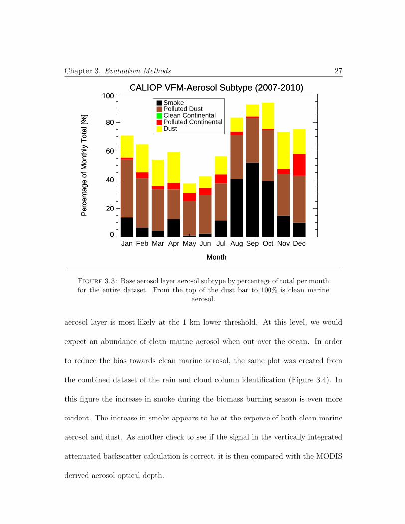
In order to use the MODIS AI data, it first had to be co-located with all columns
identified as either rainy or cloudy, in the same was as MODIS AOD. Once this
is done the monthly average aerosol optical depth can be calculated (Figure 3.8).
MODIS AI looks very similar to MODIS AOD, the only difference is that the
maximum in MODIS AI occurs in September as opposed to August. We also see
that AI starts to increase in July, much like AOD, rain/cloud total, rain/cloud
aerosol, and elevated aerosol.
3.2.4 Discussion
The 10 aerosol parameters used in this study all calculate an aerosol concentration
in a different way and over different parts of the atmosphere. To begin with, the
MODIS aerosol parameters only calculate aerosol concentration under clear sky
Chapter 3. Evaluation Methods 33
Mean Colocated MODIS Aerosol Index (2007-2010)
Jan Feb Mar Apr May Jun Jul Aug Sep Oct Nov DecMonths
0.0
0.5
1.0
1.5
2.0M
OD
IS A
ero
sol In
dex [none]
Figure 3.8: Monthly average MODIS Aerosol Index co-located with all rainyand cloudy columns in the dataset for 2007-2010.
conditions, meaning that aerosol concentration is not calculated in the presence
of clouds. Even so, the MODIS aerosol parameters may still be subject to 3-D
cloud effects and cloud contamination (Varnai and Marshak 2009; Wen et al. 2007;
Zhang et al. 2005). With that being said, the advantage to MODIS is that it
is an imager, and as such, has a much wider swath width than CALIOP since
CALIOP is an active instrument. With the wider swath width MODIS has a
greater chance of seeing clear sky in the area than CALIOP. This allows MODIS
to calculate aerosol concentration over most of the area, especially when averaged
into the 1◦x1◦ bins used by the aerosol product in this study. The first six aerosol

Chapter 3. Evaluation Methods 34
parameters calculated from the CALIOP data (equations 3.1-3.6) utilize the clear
sky identification. As a result, this data, especially when binned, can be directly
compared to the MODIS data as all eight of the calculations only calculate aerosol
concentration when looking at clear sky. This is in contrast to the last two aerosol
parameters calculated from the CALIOP data (equations 3.7 and 3.8) which look
at cloudy skies (both the rain and cloud classification). As a consequence these
parameters cannot be compared directly with all the other aerosol parameters.
Since the integrated elevated boundary layer backscatter and integrated elevated
aerosol boundary layer backscatter parameters are only calculated under cloudy
conditions, they may be missing some of the aerosol. This is especially true in the
cases when the aerosol layer is touching the cloud as a large portion of the aerosol
concentration could be below or embedded within the cloud layer. In those cases
the aerosol layers will not be calculated as the integration stops at cloud top height.
3.3 Vertical Distribution of Aerosols
Once the aerosol concentration and subtype is known, the next step is to identify
the vertical distribution of the aerosols. In order to accomplish this two differ-
ent calculations are used. The first calculation is the aerosol above cloud (AAC)

Chapter 3. Evaluation Methods 35
fraction. AAC is defined as
AAC =NAAC
NAAC + CBNA, (3.9)
where NAAC is the number of cases with aerosol above clouds and CBNA is where
there are clouds but no aerosol. In this case aerosol above clouds just means that
there is an aerosol layer present, not that the aerosol layer is greater than 250 m
above cloud top, as defined above. Therefore, this measure is used to determine
when we are most likely to find an aerosol layer. The result of this is shown in figure
Aerosol Above Cloud (2007-2010)
Jan Feb Mar Apr May Jun Jul Aug Sep Oct Nov DecMonth
0
20
40
60
80
Rat
io (
NA
AC
/(N
AA
C+
CB
NA
)) [%
] RainCloud
Figure 3.9: Monthly average aerosol above cloud fraction for 2007-2010.
3.9. First, AAC has roughly the same values for both the rainy and the cloudy
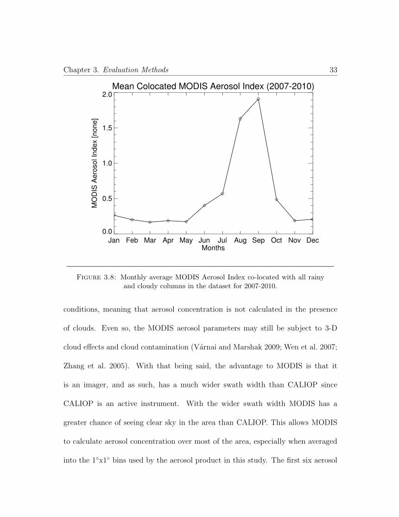
Chapter 3. Evaluation Methods 36
columns. Second, there is an increase of over 60%, from 5% to 70%, in AAC
during the biomass burning season. Interestingly, the increase begins before the
biomass burning season, in June for cloudy columns and July for rainy columns.
This corresponds to when the AI and AOD concentrations began to increase as
well.
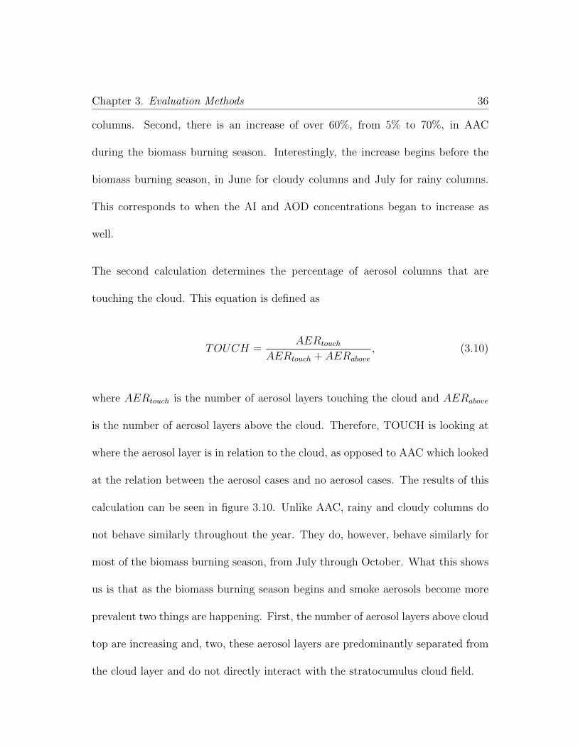
The second calculation determines the percentage of aerosol columns that are
touching the cloud. This equation is defined as
TOUCH =AERtouch
AERtouch + AERabove
, (3.10)
where AERtouch is the number of aerosol layers touching the cloud and AERabove
is the number of aerosol layers above the cloud. Therefore, TOUCH is looking at
where the aerosol layer is in relation to the cloud, as opposed to AAC which looked
at the relation between the aerosol cases and no aerosol cases. The results of this
calculation can be seen in figure 3.10. Unlike AAC, rainy and cloudy columns do
not behave similarly throughout the year. They do, however, behave similarly for
most of the biomass burning season, from July through October. What this shows
us is that as the biomass burning season begins and smoke aerosols become more
prevalent two things are happening. First, the number of aerosol layers above cloud
top are increasing and, two, these aerosol layers are predominantly separated from
the cloud layer and do not directly interact with the stratocumulus cloud field.

Chapter 3. Evaluation Methods 37
% of Aerosol Columns Touching Cloud (2007-2010)
Jan Feb Mar Apr May Jun Jul Aug Sep Oct Nov DecMonths
0
20
40
60
80A
ero
sol T
ouchin
g the C
loud [%
]
RainCloud
Figure 3.10: Monthly average aerosol touching cloud fraction for 2007-2010.
3.4 Cloud Droplet Number Concentration
CDNC (or N) is the concentration of activated CCN within a cloud. For this study,
CDNC is calculated following the formula found in Bennartz (2007). The equation
for CDNC is:
N = 2−52 τ 3(
W
CF)−52 (
3
5πQ)−3(
3
4πρl)−2c
12w, (3.11)
where W is the cloud liquid water path for a vertically homogeneous cloud, cw is
the adiabatic condensation rate, CF is the cloud fraction identified by MODIS, k
is the ratio between volume mean radius and effective radius, τ is cloud optical
depth, Q is scattering efficiency, and ρl is the density of water. For this study, k
Chapter 3. Evaluation Methods 38
and Q are assumed to be constant with values of 0.8 and 2 respectively. In addition,
cw is a function of CTT. In situ measurements of near cloud top LWC have been
found to be near 80% of the adiabatic condensation rate. As a result, the above
equations assume an 80% adiabatic condensation rate. Greater detail regarding
subadiabatic stratocumulus cloud can be found in many papers (Albrecht et al.
1990; Bretherton et al. 2004). Lastly, W is defined as:
W =5
9ρlreffτ, (3.12)
where reff is the standard MODIS derived cloud droplet effective radius retrieval.
3.5 Geometrick Thickness
Geometric thickness (H) is a useful cloud macrophysical property. Together with
CDNC, geometric thickness is a self-contained coordinate system for clouds. This is
an alternative to the cloud effective radius/COD coordinate system that is widely
used. Geometric thickness is also calculated following the formulas found in Ben-
nartz (2007). The equation for H is:
H = (2W
cwCF)12 , (3.13)
where all the variables are the same as in equation 3.11 above.

Chapter 3. Evaluation Methods 39
3.6 Effective Radius
Effective radius is another useful cloud microphysical property. For this study, the
effective radius product comes from the MODIS Collection 5 algorithms. Mathe-
matically, effective radius is defined as the ratio of the third moment to the second
moment of the cloud droplet size distribution:
re =
∞∫0
πr3n(r)dr
∞∫0
πr2n(r)dr
, (3.14)
where n(r) is the cloud droplet size distribution. However, in satellite based re-
trievals effective radius is determined based on the reflectances from two chan-
nels, one visible non-absorbing band, used mainly to calculate cloud optical depth
(COD) and one from the near-infrared, a slightly absorbing band (Twomey and
Seton 1980). The effective radius (and COD) are then determined using a look-up
table, based on work done by Nakajima and King (1990). MODIS reports three
different effective radius values based on three different channel combinations. All
three channel combinations use the 0.86 µm channel for the visible channel. The
three near- infrared channels used are 1.6, 2.1, and 3.7 µm where the 2.1 µm channel
is used in the standard MODIS effective radius retrieval.

Chapter 3. Evaluation Methods 40
3.7 Precipitation Efficiency
As a measure of precipitation efficiency this study calculated a probability of pre-
cipitation (PoP ) as a function of liquid water path. PoP is defined as:
PoP =RP
RP + CP∗ 100, (3.15)
where RP is the number of precipitating cloud columns, CP is the number of non-
precipitating cloud columns, and PoP is given as a percentage. In order to do this
calculation the LWP values are first binned. Once binned, PoP is then calculated
for each LWP bin. Additionally, the data is separated into four groups: above top,
above bottom, touch top, and touch bottom. The above groups have aerosol layers
above the cloud, whereas the touch groups have aerosol layers touching the clouds.
The top and bottom groups are for the top and bottom 20% of aerosol cases
respectively. This calculation is then carried out for all ten aerosol calculations
presented earlier. Results of this calculation will be shown in Chapter 4.

Chapter 4. Results 41
Chapter 4
Results
4.1 Aerosol Metrics
4.1.1 Statistical Analysis
We would expect that most of the aerosol parameters would correlate well with
each other. For example, AI, AOD, and CLEARTOTAER should correlate ex-
tremely well with each other since these three parameters are looking at the aerosol
concentration of the column. CLEARTOT should correlate well with these param-
eters as well since aerosols should be the biggest contribution to the vertically
integrated attenuated backscatter since there should not be any other particles in
the atmosphere that would have a large extinction cross-section. CLEARVIAB,

Chapter 4. Results 42
CLEARAERVIAB, CLEARLOW, CLEARLOWAER, VIAB, and AERVIAB may
not correlate as well given the fact that these parameters will not integrate through
the entire atmosphere and may miss aerosol layers. However, the four elevated cal-
culations should correlate well in areas where there is minimal aerosol in the lowest
one kilometer and CLEARLOW and CLEARLOWAER should correlate well when
there is not an aerosol layer above one kilometer. As we have already seen, and
will be shown quantitatively below, the correlation between the aerosol parameters,
in many cases, is not as strong as one would expect. In order to isolate various
aerosol effects and remove the confounding influence of meteorological properties,
this study divided the data into 12 subsets. First, the data was previously divided
into rainy and cloudy columns with the columns containing an aerosol layer iden-
tified. Next it was determined if the aerosol layer was above the cloud or touching
the cloud. Again, a difference in aerosol base height and cloud top height of 250
m is the point at which this study divides the aerosol layers between touching
and being above the cloud. At this point, there are four subsets within the data.
Within each subset the top, middle, and bottom 10% of all liquid water path values
were determined. LWP was calculated using equation 3.12. In the following figures
these 12 subsets will be identified as: rain, above, top (RAT); rain, above, middle
(RAM); rain, above, bottom (RAB); rain, touch, top (RTT); rain, touch, middle
(RTM); rain, touch, bottom (RTB); cloud, above, top (CAT); cloud, above, mid-
dle (CAM); cloud, above, bottom (CAB); cloud touch top (CTT); cloud, touch,
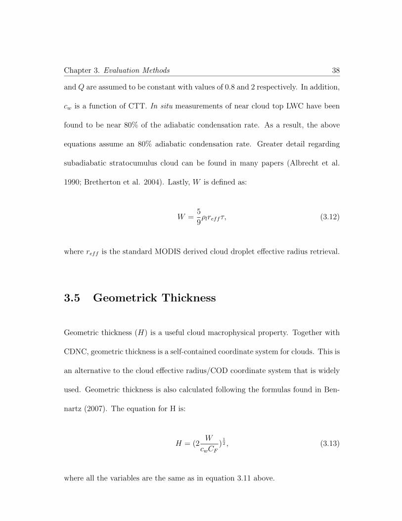
Chapter 4. Results 43
middle (CTM); and cloud, touch, bottom (CTB). For each set of parameters a
linear fit was calculated. Unless otherwise noted, all correlations shown below are
statistically significant at or above 0.95.
The first set of correlations that will be shown is AI vs. CLEAERAERVIAB
(Figure 4.1). This is a case where the correlations are moderately high. While
Figure 4.1: AI vs. CLEARAERVIAB for RAT (A), CAT (B), RAB (C), andCAM (D).
this combination of aerosol parameters does not have the highest correlations (AI
vs. AERVIAB has the highest) this combination of aerosol metrics has a fairly
consistent trend between the parameters as evidenced by the slope of the linear fit.
The fact that AI vs. CLEARAERVIAB has such a consistent set of correlations and
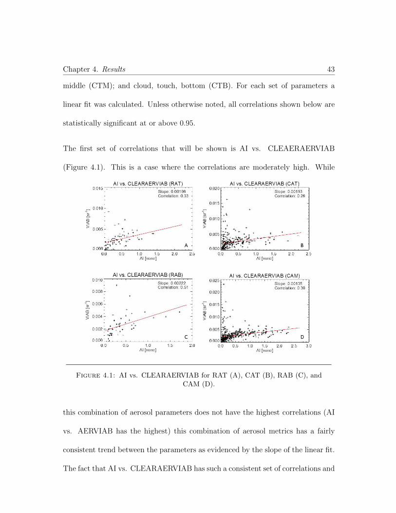
Chapter 4. Results 44
slopes suggests that AI may be more representative of elevated aerosol layers than
boundary layer aerosol layers. This point is further supported by the fact that the
correlation between AI and AERVIAB is 0.46 (RAT), 0.30 (RAB), 0.44 (CAT), and
0.58 (CAM). Interestingly, AOD vs. CLEARTOTAER is one of the combinations
that has poor correlations, especially in terms of consistency between subsets of the
data. Out of the 12 categories, only two have statistically significant correlations,
CAM (-0.09) and CAB (-0.1). Further supporting the fact that AI may not be
representative of the boundary layer aerosol layer is that the correlations between
AI and CLEARLOWAER are moderate and negative (Figure 4.2). Not only are
Figure 4.2: AI vs. CLEARLOWAER for RAT (A), CAM (B), CTB (C), andCAB (D).

Chapter 4. Results 45
the correlations negative, they are consistent as well. In these cases the slope
between the parameters is consistent as well. While an argument could be made
that CLEARLOW and CLEARLOWAER could have a negative slope, it is less clear
that this argument can be made for CLEARTOT or CLEARTOTAER. Looking at
figure 3.1, however, one notices that low aerosol appears to account for a majority
of the total aerosol concentration during the months of January through March
and October through December while the elevated aerosol contribution starts to
become significant for the months of June through September when it surpasses the
low aerosol contribution. Given this, it seems more plausible that there could be a
negative correlation between AOD and CLEARTOTAER. It is interesting to note
that elevated aerosol becomes the significant contribution to total aerosol during
the biomass burning months.
Another way to look at the data is to try and determine if the trends within any of
the subsets are robust. Looking at the trends in CTT for various aerosol parameter
combinations (Figure 4.3), we see that this is a case where the correlation between
the aerosol parameters is consistently positive and quite strong for AI and AOD
vs. AERVIAB. Additionally, the slopes of the linear fit are similar to one another,
especially for AI and AOD vs. AERVIAB and AI and AOD vs. CLEARAERVIAB.
It is promising to see that the stronger correlations correspond with the steeper
slopes. With that being said, the fact remains that there is a wide spread in the
correlations within this subset of the data. Unfortunately, as was the case when

Chapter 4. Results 46
Figure 4.3: Cloud, Touch, Top for AI vs.AERVIAB (A), AOD vs. AERVIAB(B), AI vs. CLEARAERVIAB (C), and AOD vs. CLEARAERVIAB (D).
looking at aerosol parameter combinations, there are also inconsistent correlations
within a subset of the data as well (Figure 4.4). In this case AI vs. AERVIAB
(RAM) and AOD vs. CLEARAERVIAB (RAM) have a positive correlation while
AOD vs. CLEARTOT (RAM) and AOD vs. CLEARLOWAER (RAM) have a
negative correlation. The one promising aspect of the figure though is that is that
we would not necessarily expect CLEARLOWAER to have as strong of a correla-
tion with AI or AOD. With that being said, it is unclear whether this relationship
should exhibit a negative correlation. In addition, there is a negative correlation
between AOD and CLEARTOT. However, even if the negative correlations are
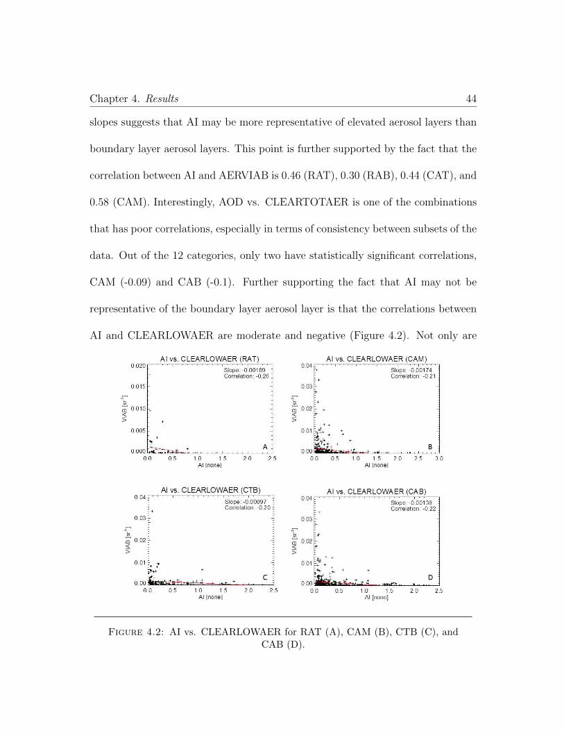
Chapter 4. Results 47
Figure 4.4: Rain, Above, Middle for AI vs. AERVIAB (A), AOD vs.CLEARTOT (B), AOD vs. CLEARAERVIAB (C), and AOD vs. CLEAR-
LOWAER (D).
thrown out, assuming negative correlations are not physical, the correlation be-
tween the aerosol parameters within the CTT subset is weak and varied with the
strongest correlation being 0.52 from the AI vs. AERVIAB combination and the
weakest positive correlation being 0.15 from the the AOD vs.VIAB combination
(not shown). This is a large difference when some of the correlations are not strong
to begin with.
While the correlation between the various aerosol parameters are not great there
is some hope that the aerosol metrics presented may be able to pick out a signal
relating to the aerosol indirect and semi-direct effects. There are a number of
Chapter 4. Results 48
combinations that show promise, AI vs. AERVIAB and CLEARVIAB as well as
AOD vs. AERVIAB and CLEARAERVIAB.
It is interesting to note that in cloudy columns the only combinations that have a
negative correlation integrate through the lowest 1 km. The same can be said for
rainy columns, with CLEARVIAB also having a negative correlation with AI for
the RAT subset. There are a number of possible explanations for how a negative
correlation can make physical sense. First, it is plausible that either MODIS does
a better job with elevated aerosol layers or that CALIOP cannot accurately see
aerosols in the lowest one kilometer. Second, it is possible that the aerosol layers
in the lowest one kilometer, while significant, are optically thin and below the
detection limit of MODIS.
4.1.2 Case Studies
Two case studies are presented below. For each case study a map of the region
is shown with the aerosol concentration plotted on a map with a line overlaid
indicating the satellite track, a profile of the CALIOP derived aerosol parameter
plotted versus latitude and CALIOP backscatter and vertical feature mask profiles
for that case. The profile of the CALIOP derived aerosol parameter will calculate
the parameter for that column specifically, it will not be the 1◦x1◦ average. The
columns identified as rainy, cloudy, and clear will be identified. The first case
Chapter 4. Results 49
study consists of two aerosol parameters that have a strong correlation, AI and
CLEARAERVIAB for August 7, 2010. The second case study consists of two
aerosol parameters that have a weak correlation, AI and CLEARLOWAER for
November 16, 2007.
4.1.2.1 Case Study 1
Shown in figure 4.5 is the CALIOP 1064 nm attenuated backscatter for August 7,
Figure 4.5: CALIOP 1064 Attenuated Backscatter for August 7, 2010 with thearea of interest outlined in red.
2010 with the area of interest outlined in red. The left side of the figure, left of
latitude -12.86◦ N, the satellite track is over land. Over the ocean we see a fairly
persistent stratocumulus cloud layer, except for a region centered around -6.75◦
N. Centered over the same region there appears to be a fairly thick aerosol layer
that extends over the cloud layer. From figure 4.6 we see that the aerosol layer, at

Chapter 4. Results 50
Figure 4.6: CALIOP VFM overlying 1064 Total Attenuated Backscatter forAugust 7, 2010 for the area of interest. Dark Blue-Clear Sky, Light Blue-Cloud, Orange-Aerosol, Green-Surface, Grey-Subsurface, Black-Totally Atten-
uated, Red-Cloud Low/No Confidence, Brown-Aerosol Low/No Confidence
least in terms of the scene classification algorithm, appears to be above the cloud
layer in most, if not all, locations. From this figure it appears that the vertical
feature mask is missing the bottom portion of the aerosol layer. This appears
most obvious in the cloud free region left of the area identified as aerosol low/no
confidence (brown). If CALIOP systematically misses the bottom of the aerosol
layers, like it does in this case, this could have implications for the aerosol metrics
that only integrate through aerosol layers.
Quantifying the aerosol concentration (Figure 4.7) we see that the aerosol con-
centration increases as one goes north for both CLEARAERVIAB and AI. In this
case at least, CLEARAERVIAB appears to have a larger gradient in aerosol con-
centration than AI. From the MODIS AI data we can see that most of the study
area is characterized by low background aerosol concentrations with pockets of en-
hanced aerosol concentrations. Looking at the profile of AERVIAB, there is clearly

Chapter 4. Results 51
August 7, 2010-AERVIAB
-20 -15 -10 -5Latitude [deg]
0.000
0.002
0.004
0.006
0.008
0.010
0.012V
IAB
[sr-1
]AllRainCloudClear
CLEARAERVIAB [sr-1]
-10 -5 0 5 10 15
-25
-20
-15
-10
-5
0
10
20
30
40
51
61
x104
AI [none]
-10 -5 0 5 10 15
-25
-20
-15
-10
-5
0
5
10
16
21
26
31
x10
Figure 4.7: Map of aerosol concentration for August 7, 2010. Profile ofAERVIAB (Top), map of CLEARAERVIAB (Bottom Left), map of AI (Bot-
tom Right)
an increasing trend in aerosol concentration as the satellite moves north over the
ocean. Over land there appears to be more of a constant aerosol concentration. It
is important to note that from about -12◦ to about -8◦ N latitude the columns are
identified as cloudy only and from about -8◦ to -5◦ N the columns are identified
mainly as clear. Recall that CLEARAERVIAB, the variable that we are using in
this case study, calculates aerosol concentration solely under clear sky conditions.
This is why the map of CLEARAERVIAB does not have data south of -8◦ N. As
a consequence, none of the cloudy columns will have a valid aerosol concentration
in this case as there is not a clear sky column within the 1◦x1◦ grid cell necessary
for a retrieval of aerosol concentration. Therefore, most of the cloud microphysical
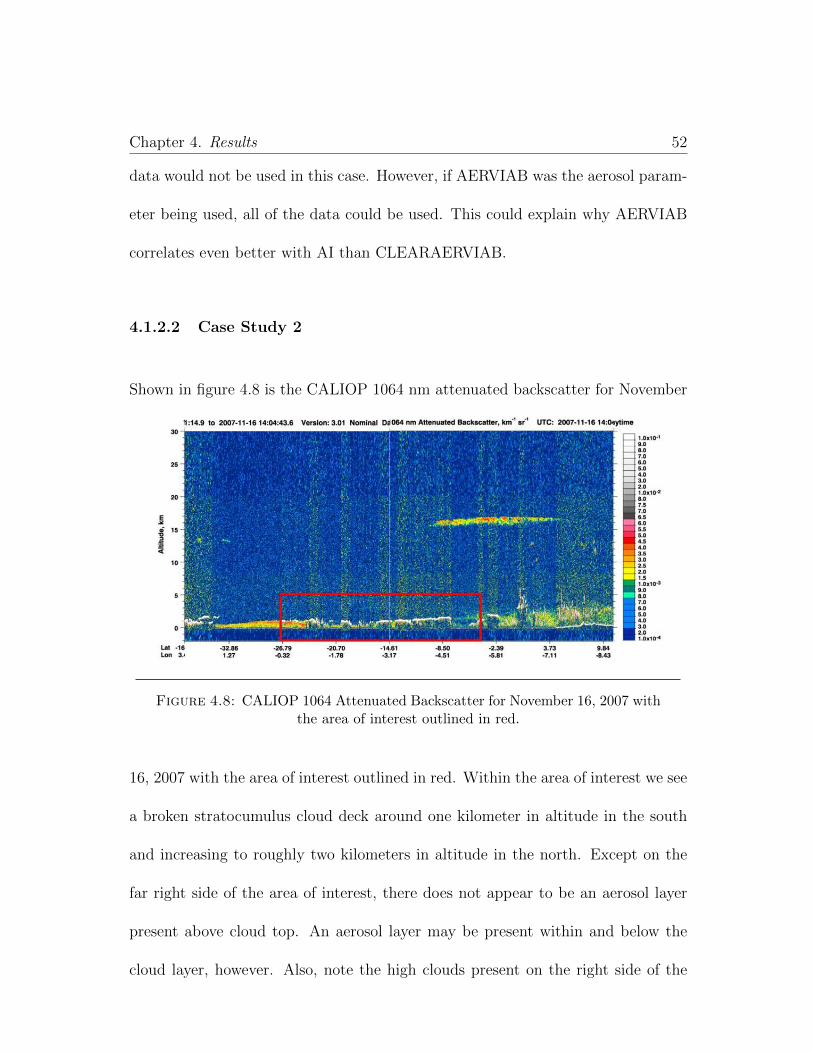
Chapter 4. Results 52
data would not be used in this case. However, if AERVIAB was the aerosol param-
eter being used, all of the data could be used. This could explain why AERVIAB
correlates even better with AI than CLEARAERVIAB.
4.1.2.2 Case Study 2
Shown in figure 4.8 is the CALIOP 1064 nm attenuated backscatter for November
Figure 4.8: CALIOP 1064 Attenuated Backscatter for November 16, 2007 withthe area of interest outlined in red.
16, 2007 with the area of interest outlined in red. Within the area of interest we see
a broken stratocumulus cloud deck around one kilometer in altitude in the south
and increasing to roughly two kilometers in altitude in the north. Except on the
far right side of the area of interest, there does not appear to be an aerosol layer
present above cloud top. An aerosol layer may be present within and below the
cloud layer, however. Also, note the high clouds present on the right side of the

Chapter 4. Results 53
image, near -8◦ N. Areas with high altitude clouds are not included in the dataset.
Looking at figure 4.9, the vertical feature mask agrees with the assessment of this
Figure 4.9: CALIOP VFM overlying 1064 Total Attenuated Backscatter forNovember 16, 2007 for the area of interest. Dark Blue-Clear Sky, Light Blue-Cloud, Orange-Aerosol, Green-Surface, Grey-Subsurface, Black-Totally Attenu-
ated
scene. Most of the aerosol lies within the clear sky region on the right side of the
area of interest. The vertical feature mask also identifies an aerosol layer below
the cloud throughout most of the area of interest. Recall that this aerosol layer is
ignored in the analysis, only aerosol layers above cloud top are identified as aerosol
layers below cloud top cannot be reliably retrieved.
Quantifying the aerosol concentration (Figure 4.10) we immediately notice the very
poor correlation between CLEARLOWAER and AI. CLEARLOWAER retrieves a
high aerosol concentration to the south of -15◦ N while the AI data is fairly consis-
tent along the satellite overpass track. AI also identifies a much more widespread
aerosol layer, both on and off the satellite overpass track. In this case CALIOP
must not be correctly identifying the aerosol layer as there are a lot of clear sky
pixels identified in the satellite overpass, as seen in the top portion of figure 4.10.
There is also the possibility that MODIS AI is too high, especially if the cloud
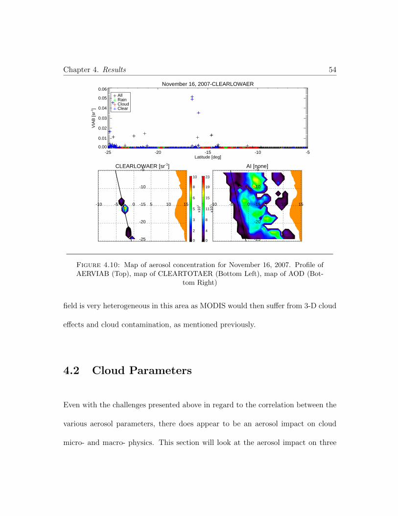
Chapter 4. Results 54
November 16, 2007-CLEARLOWAER
-25 -20 -15 -10 -5Latitude [deg]
0.00
0.01
0.02
0.03
0.04
0.05
0.06V
IAB
[sr-1
]AllRainCloudClear
CLEARLOWAER [sr-1]
-10 -5 0 5 10 15
-25
-20
-15
-10
-5
0
2
3
5
6
8
10
x103
AI [none]
-10 -5 0 5 10 15
-25
-20
-15
-10
-5
0
4
8
11
15
19
23
x102
Figure 4.10: Map of aerosol concentration for November 16, 2007. Profile ofAERVIAB (Top), map of CLEARTOTAER (Bottom Left), map of AOD (Bot-
tom Right)
field is very heterogeneous in this area as MODIS would then suffer from 3-D cloud
effects and cloud contamination, as mentioned previously.
4.2 Cloud Parameters
Even with the challenges presented above in regard to the correlation between the
various aerosol parameters, there does appear to be an aerosol impact on cloud
micro- and macro- physics. This section will look at the aerosol impact on three

Chapter 4. Results 55
parameters: cloud droplet number concentration, effective radius, and the proba-
bility of precipitation.
4.2.1 Cloud Droplet Number Concentration
Shown in figure 4.11 is CDNC plotted against one of the aerosol parameters. The
Figure 4.11: Cloud Droplet Number Concentration. AOD vs. CDNC(RTB)(A), AI vs. CDNC (CTT)(B), CLEARVIAB vs. CDNC (RTB)(C), AOD
vs. CDNC (CTT)(D)
left two figures, figures A and C, have much higher correlations and steeper slopes
than the two figures on the right. With that being said, the fact that all four figures
show a consistent positive trend leads one to believe that an increase aerosol con-
centration does lead to an increase in CDNC. These data suggest, however, that we
should be cautious when trying to quantify the exact relationship between aerosol

Chapter 4. Results 56
concentration and CDNC given that the slopes and correlations vary, even within
this subset. Bearing that in mind, these plots still show results that are consistent
with the first indirect aerosol effect. The remaining statistically significant aerosol
vs. CDNC scatter plots can be found in Appendix A.
4.2.2 Effective Radius
Looking at figure 4.12 is the effective radius plotted against one of the aerosol pa-
Figure 4.12: Effective Radius. CLEARLOWAER vs. Effective Radius(RAT)(A), AI vs. Effective Radius (CTT)(B), CLEARVIAB vs. Effective Ra-
dius (RTB)(C), AOD vs. Effective Radius (CTT)(D)
rameters. Three of the four figures (A, B, and D) have very similar correlations,
with figure D having a much lower correlation than the other three. While three of

Chapter 4. Results 57
the correlations may be similar, there is still a significant variation in the correla-
tion, as well as the slope, between the various combinations shown. As was the case
with CDNC, we should be cautious when trying to quantify the exact relationship
between aerosol concentration and effective radius given the spread in correlations
and slopes. Again though, these plots point to the fact that an increase in aerosol
concentration leads to a decrease in effective radius, results consistent with the first
indirect aerosol effect. The remaining statistically significant aerosol vs. effective
radius scatter plots can be found in Appendix A.
4.2.3 Probability of Precipitation
Shown in figure 4.13 is the probability of precipitation (PoP) for four different
Figure 4.13: Probability of Precipitation. AOD (A), AI (B), CLEAR-AERVIAB (C), CLEARLOWAER(D)

Chapter 4. Results 58
aerosol metrics. These plots are different from the previous plots shown. The
x-axis is now LWP, not aerosol concentration. The top and bottom, in this case
then, represent the top and bottom 20% aerosol concentration values for whatever
aerosol metric is being used. The top two figures, AI and AOD, show an increase
in PoP with an increase in aerosol above the cloud, especially at the higher liquid
water path values. An increase in aerosol above the cloud layer would increase
the temperature of the atmospheric layer. This would increase the strength of the
inversion capping the stratocumulus cloud layer. This would then further limit
cloud growth. With constant LWP, a cloud should precipitate more efficiently if
it is thinner as there is a greater chance of collision between the cloud droplets,
increasing the efficiency of the collision-coalescence process. Note that this is not
the semi-direct effect where liquid water path is expected to decrease in the pres-
ence of aerosols. CLEARAERVIAB shows an increase in PoP with decreasing
aerosol concentration above the cloud. An explanation for this discrepancy was
not found. AOD, CLEARAERVIAB, and especially CLEARLOWAER show a de-
crease in PoP with an increase in aerosol concentration when the aerosol layer is
touching the cloud. This is consistent with the first and second indirect aerosol
effects. CLEARLOWAER should be especially sensitive to this change as this is
the aerosol layer that would get ingested into the cloud through updrafts, not just
entrainment through turbulent mixing at cloud top, as is the case with the aerosol
layers that are touching the cloud from above. Since all CCN do not become cloud
Chapter 4. Results 59
droplets, the ingestion of aerosol at cloud base would increase the amount of time
that an aerosol has to become activated and form a cloud droplet. AI shows an
increase in PoP with an increase in aerosol concentration touching the cloud. An
explanation for the discrepancy between AI and the other three aerosol parameters
shown has not been found. The PoP for the other six aerosol parameters are shown
in Appendix B.
4.3 Challenges
Almost every result shown has had either varying correlations and slopes or con-
tradictory results. In many cases an attempt was made to identify some of the
challenges associated with that data and a possible explanation. This section will
highlight some of these challenges, as well as many new ones, that have been doc-
umented in the literature that could have an affect on the results shown.
Haywood et al. (2004) found that aerosols located above cloud layers may affect
the COD and effective radius retrievals from MODIS. Using the default MODIS
channel combination of 0.86 µm and 2.1 µm, COD is more affected by aerosol
overlying a cloud than effective radius. In cases with an overlying aerosol layer the
COD will be underestimated, the amount determined by the AOD of the aerosol
layer. An error in COD could affect the results of this study in multiple ways. First,
COD is used in scene classification. If COD is underestimated this study could be
Chapter 4. Results 60
throwing out legitimate rainy and cloudy cases that did not meet this threshold.
Second, COD is then used as input into the equations for LWP and CDNC. LWP is
also a variable in the equation for CDNC. Therefore, underestimating COD could
lead to more data being thrown out, a decrease in LWP, and an increase in CDNC.
The quantitative effects this could have are beyond the scope of this study.
Breon and Doutriaux-Boucher (2005) found that the MODIS effective radius re-
trieval is sensitive to cloud heterogeneity. A decrease in cloud fraction (increase in
cloud heterogeneity) leads to an overestimation of the effective radius. Given the
heterogeneity of the stratocumulus cloud layer in this area, this most likely has an
have an affect on the effective radius in this study. In turn, this could lead to an
overestimation the liquid water path calculation and CDNC calculation.
Kacenelenbogen et al. (2014) found that CALIOP, when compared with High Spec-
tral Resolution Lidar from NASA Langley, detects only 23% of AAC cases. The
study found that the underestimation of AAC is the result of extremely thin aerosol
layers (τ > 0.02) that fall below the detection limit of CALIOP. Another explana-
tion for the underestimation of AAC by CALIOP is incorrect aerosol type classifi-
cation (Omar et al. 2009). This could be caused by low signal-to-noise ratio or the
use of loading-dependent lidar measurements that are only loosely related to aerosol
type. If the same statistics hold for the southeastern Atlantic Ocean, this could
explain the low fraction of rainy (25%) and cloudy (28%) that have an aerosol layer

Chapter 4. Results 61
above cloud top in this study. Better detection of AAC layer would lead to more
accurate integrated backscatter values when integrating through aerosol layers.
Another potential source of error between MODIS and CALIOP derived aerosol
concentration is that in AOD retrievals MODIS assumes a value for aerosol ab-
sorption. However, Eck et al. (2013) found that this assumption leads to a single
scatter albedo induced bias within the MODIS AOD retrieval as the study found
a seasonal cycle in single scatter albedo in southwestern Africa. The single scatter
albedo increases from 0.81 in July to 0.92 in November, which leads to a factor of
2 difference in optical depth as a result of absorption.
Winker et al. (2009) also lists possible sources of error in the calculation of CALIOP
AOD. Possible sources of error include: instrument calibration and normalization
errors, errors in cloud-aerosol discrimination, layer boundary detection, multiple
scattering, and a priori lidar ratios. Tanre et al. (1997) had previously identified
possible sources of error in the calculation of AOD from MODIS. The sources of
error include: surface reflection, sensor calibration, contamination by glint, water-
leaving radiance, and uncertainties involved in the lookup tables such as aerosol
size distribution, refractive index, and single-scattering albedo. Depending on the
situation where each type of error could occur, this could contribute to the low cor-
relation between the MODIS derived and CALIOP derived aerosol concentrations.
With regard to aerosol misclassification, Kim et al. (2013) found that the large
difference in biomass burning AOD between MODIS and CALIOP is the result of
Chapter 4. Results 62
incorrect identification of aerosol layer base altitude. In that study it was shown
that most CALIOP AOD does not extend into the marine boundary layer, leading
to an underestimation of CALIOP AOD. Evidence of this was seen in Case Study
1 where the bottom of the aerosol layer did not appear to be identified by the
CALIOP vertical feature mask.
Another possible challenge in assessing the affect of aerosols on clouds is the hygro-
scopicity of aerosols. As humidity increases aerosols tend to swell, the amount of
swelling is dependent on the hygroscopic properties of the specific aerosol. Twohy
et al. (2009) showed that an increase in relative humidity causes the aerosol parti-
cle to grow, subsequently causing the scattering cross-section to increase. In turn,
this increases the apparent aerosol concentration retrieved from satellites. An in-
crease in aerosol concentration with increasing cloud cover has been reported in
many satellite-based studies (Ignatov et al. 2005; Kaufman et al. 2005; Koren et al.
2007; Loeb and Manalo-Smith 2005; Loeb and Schuster 2008; Matheson et al. 2006;
Quaas et al. 2008; Sekiguchi et al. 2003). As a consequence, hygroscopic swelling
of aerosols could play an important role in the results of this study.
Additionally, aerosol and cloud parameters may co-vary as a result of meteorological
conditions. In some cases, changes in meteorological conditions may be greater
than the aerosol induced changes (e.g. Petters et al. 2013). Another challenge
noticed in this study is that clear-sky columns may not be spatially located near
the clouds being studied. This was seen in Case Study 1 where there was a 4◦

Chapter 4. Results 63
range of cloud columns identified without a single clear column identified. As a
consequence, none of the cloud data could be used with the MODIS or CALIOP
clear-sky derived aerosol parameters. North of -8◦ N there was a range of clear
columns with very limited cloud columns in the area. In this case, most of the
aerosol data would go unused as there was not a cloud nearby to assign to the
aerosol concentration.
Chapter 5. Conclusions 64
Chapter 5
Conclusions
This study has shown that the correlation between aerosol metrics varies greatly.
The correlations between AI and CLEARAERVIAB (R: 0.14-0.51), AI and AERVIAB
(R: 0.28-0.58), AOD and CLEARAERVIAB (R: 0.15-0.34), and AOD and AERVIAB
(R: 0.11-0.6) are moderate while the correlations between AI and CLEARLOWAER
(R: -0.27-(-0.18)) and AOD and CLEARLOWAER (R: -0.26-(-0.16)) are quite low.
A number of possible explanations regarding the lack of a strong correlation were
presented in detail in the previous section. There are multiple explanations re-
garding the low correlation between AI, AOD, and CLEARLOWAER. First, it is
possible that CALIOP cannot accurately sense aerosols in the lowest one kilome-
ter. While it is true that CPR aboard CloudSat has this issue there is no reason to
believe this is the case with CALIOP, especially over the depth of one kilometer.

Chapter 5. Conclusions 65
Second, MODIS may have trouble viewing aerosols in the lowest one kilometer. As
MODIS is a passive instrument, this should not be a major issue. Lastly, aerosol
layers in the lowest one kilometer can be extremely thin, potentially below the
detection limit of MODIS. Of the three possibilities, this las option seems the most
promising.
One other possible issue is that in AOD retrievals MODIS assumes a value for
aerosol absorption. However, Eck et al. (2013) found that the single scatter albedo
increases from 0.81 in July to 0.92 in November, which leads to a factor of 2
difference in optical depth as a result of absorption.
In many cases different aerosol metrics can give vastly different results, in some
cases even the sign of the trend can change. This was the case when four combi-
nations of aerosol metrics were shown for the subset RAM (Figure 4.4). In this
case the correlation between the aerosol parameters ranged form R = −0.26 to
R = 0.52. When such a large range is present, it is harder to trust the data. How-
ever, there is still a possibility that the trends are real as the negative correlations
involve CLEARLOWAER and CLEARTOT. As just mentioned, there could be a
physical explanation for the negative correlation. It is this type of result, how-
ever, that leads to some of the challenges one encounters when trying to assess the
aerosol indirect and semi-direct effects.
Even with the challenges associated with this type of study there appears to be an
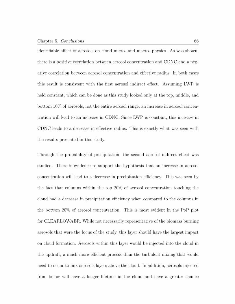
Chapter 5. Conclusions 66
identifiable affect of aerosols on cloud micro- and macro- physics. As was shown,
there is a positive correlation between aerosol concentration and CDNC and a neg-
ative correlation between aerosol concentration and effective radius. In both cases
this result is consistent with the first aerosol indirect effect. Assuming LWP is
held constant, which can be done as this study looked only at the top, middle, and
bottom 10% of aerosols, not the entire aerosol range, an increase in aerosol concen-
tration will lead to an increase in CDNC. Since LWP is constant, this increase in
CDNC leads to a decrease in effective radius. This is exactly what was seen with
the results presented in this study.
Through the probability of precipitation, the second aerosol indirect effect was
studied. There is evidence to support the hypothesis that an increase in aerosol
concentration will lead to a decrease in precipitation efficiency. This was seen by
the fact that columns within the top 20% of aerosol concentration touching the
cloud had a decrease in precipitation efficiency when compared to the columns in
the bottom 20% of aerosol concentration. This is most evident in the PoP plot
for CLEARLOWAER. While not necessarily representative of the biomass burning
aerosols that were the focus of the study, this layer should have the largest impact
on cloud formation. Aerosols within this layer would be injected into the cloud in
the updraft, a much more efficient process than the turbulent mixing that would
need to occur to mix aerosols layers above the cloud. In addition, aerosols injected
from below will have a longer lifetime in the cloud and have a greater chance

Chapter 5. Conclusions 67
of being activated and become CCN. There could also be an effect of aerosol on
PoP when the aerosol layer is above cloud top, instead of touching cloud top.
In this case it looks like there is an increase in PoP with an increase in aerosol
concentration, especially at larger LWP values. The aerosol layers above the cloud
should increase the temperature of that layer as a result of absorption. This should
strengthen the inversion capping the stratocumulus cloud layer. The cloud would
then precipitate more efficiently as the same LWP is confined to a smaller area,
increasing the efficiency of the collision-coalescence process. As mentioned earlier,
the analysis presented cannot diagnose the semi-direct effect as liquid water path
should decrease in the presence of an absorbing aerosol layer above cloud top and
this analysis is done with liquid water path held constant.
To study the effect of aerosol above clouds, future studies should subset the dataset
further and divide the above cloud subset into multiple levels. For example, it
seems unreasonable to think that an aerosol layer three kilometers above cloud
top would have the same effect on cloud macro- and micro- physics as an aerosol
layer only a kilometer above cloud top. In this study however, both sets of cases
would have been combined into a single subset. Future studies should also include
the CALIPSO Lidar Cloud and Aerosol Discrimination (CAD) score. Inclusion of
the CAD score would be a further guarantee that clouds and aerosols are properly
identified within the dataset.
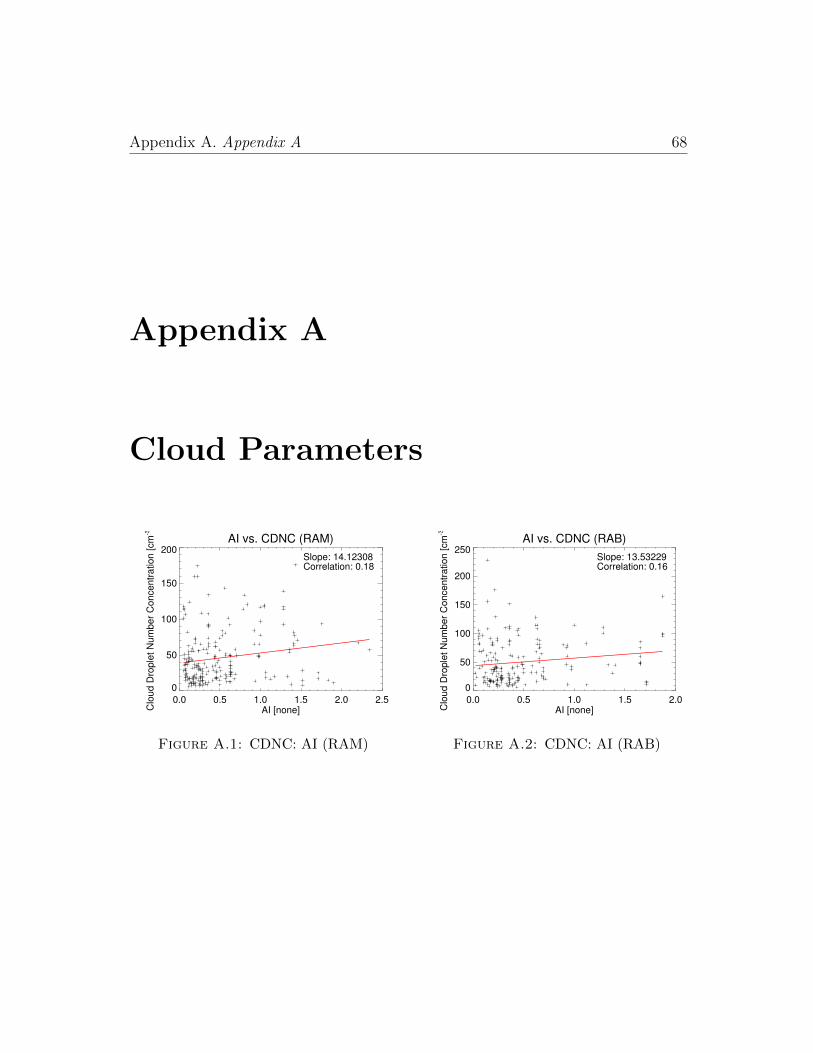
Appendix A. Appendix A 68
Appendix A
Cloud Parameters
AI vs. CDNC (RAM)
0.0 0.5 1.0 1.5 2.0 2.5AI [none]
0
50
100
150
200
Clo
ud D
rople
t N
um
ber
Concentr
ation [cm
-3]
Slope: 14.12308Correlation: 0.18
Figure A.1: CDNC: AI (RAM)
AI vs. CDNC (RAB)
0.0 0.5 1.0 1.5 2.0AI [none]
0
50
100
150
200
250
Clo
ud D
rople
t N
um
ber
Concentr
ation [cm
-3]
Slope: 13.53229Correlation: 0.16
Figure A.2: CDNC: AI (RAB)

Appendix A. Appendix A 69
AI vs. CDNC (RTT)
0.0 0.2 0.4 0.6 0.8AI [none]
0
50
100
150
200
250
300
Clo
ud D
rople
t N
um
ber
Concentr
ation [cm
-3]
Slope: 198.24744Correlation: 0.47
Figure A.3: CDNC: AI (RTT)
AI vs. CDNC (RTB)
0.0 0.2 0.4 0.6 0.8 1.0AI [none]
0
50
100
150
200
250
Clo
ud D
rople
t N
um
ber
Concentr
ation [cm
-3]
Slope: 134.17123Correlation: 0.40
Figure A.4: CDNC: AI (RTB)
AI vs. CDNC (CAT)
0.0 0.5 1.0 1.5 2.0 2.5AI [none]
0
100
200
300
400
Clo
ud D
rople
t N
um
ber
Concentr
ation [cm
-3]
Slope: 10.15579Correlation: 0.08
Figure A.5: CDNC: AI (CTT)
AI vs. CDNC (CAM)
0.0 0.5 1.0 1.5 2.0 2.5 3.0AI [none]
0
200
400
600
Clo
ud D
rople
t N
um
ber
Concentr
ation [cm
-3]
Slope: 31.54023Correlation: 0.16
Figure A.6: CDNC: AI (CAM)
AI vs. CDNC (CAB)
0.0 0.5 1.0 1.5 2.0 2.5AI [none]
0
200
400
600
Clo
ud D
rople
t N
um
ber
Concentr
ation [cm
-3]
Slope: 23.41637Correlation: 0.14
Figure A.7: CDNC: AI (CAB)
AI vs. CDNC (CTM)
0.0 0.5 1.0 1.5 2.0 2.5AI [none]
0
100
200
300
400
500
600
Clo
ud D
rople
t N
um
ber
Concentr
ation [cm
-3]
Slope: 45.35008Correlation: 0.18
Figure A.8: CDNC: AI (CTM)

Appendix A. Appendix A 70
AOD vs. CDNC (RAM)
0 1 2 3 4 5AOD [none]
0
50
100
150
200
250
Clo
ud D
rople
t N
um
ber
Concentr
ation [cm
-3]
Slope: 12.26459Correlation: 0.15
Figure A.9: CDNC: AOD(RAM)
AOD vs. CDNC (RTT)
0.0 0.2 0.4 0.6 0.8AOD [none]
0
50
100
150
200
250
300
Clo
ud D
rople
t N
um
ber
Concentr
ation [cm
-3]
Slope: 257.36767Correlation: 0.48
Figure A.10: CDNC: AOD(RTT)
AOD vs. CDNC (CAM)
0 1 2 3 4 5AOD [none]
0
200
400
600
Clo
ud D
rople
t N
um
ber
Concentr
ation [cm
-3]
Slope: 18.98351Correlation: 0.15
Figure A.11: CDNC: AOD(CAM)
AOD vs. CDNC (CAB)
0 1 2 3 4 5AOD [none]
0
200
400
600
Clo
ud D
rople
t N
um
ber
Concentr
ation [cm
-3]
Slope: 19.58331Correlation: 0.14
Figure A.12: CDNC: AOD(CAB)
AOD vs. CDNC (CTM)
0 1 2 3 4 5AOD [none]
0
100
200
300
400
500
600
Clo
ud D
rople
t N
um
ber
Concentr
ation [cm
-3]
Slope: 35.78161Correlation: 0.13
Figure A.13: CDNC: AOD(CTM)
AERVIAB vs. CDNC (CAT)
0.000 0.002 0.004 0.006 0.008 0.010 0.012VIAB [sr-1]
0
100
200
300
400
Clo
ud D
rople
t N
um
ber
Concentr
ation [cm
-3]
Slope: 763.88886Correlation: 0.03
Figure A.14: CDNC: AERVIAB(CAT)

Appendix A. Appendix A 71
AERVIAB vs. CDNC (CAM)
0.000 0.005 0.010 0.015 0.020VIAB [sr-1]
0
100
200
300
400
500
600
Clo
ud D
rople
t N
um
ber
Concentr
ation [cm
-3]
Slope: 4039.90487Correlation: 0.10
Figure A.15: CDNC: AERVIAB(CAM)
AERVIAB vs. CDNC (CAB)
0.000 0.005 0.010 0.015 0.020 0.025VIAB [sr-1]
0
200
400
600
800
Clo
ud D
rople
t N
um
ber
Concentr
ation [cm
-3]
Slope: 6212.61023Correlation: 0.13
Figure A.16: CDNC: AERVIAB(CAB)
VIAB vs. CDNC (RAT)
0.000 0.005 0.010 0.015 0.020 0.025VIAB [sr-1]
0
50
100
150
200
250
Clo
ud D
rople
t N
um
ber
Concentr
ation [cm
-3]
Slope: 2773.71580Correlation: 0.18
Figure A.17: CDNC: VIAB(RAT)
VIAB vs. CDNC (RAM)
0.000 0.005 0.010 0.015 0.020 0.025 0.030VIAB [sr-1]
0
50
100
150
200
250
300
Clo
ud D
rople
t N
um
ber
Concentr
ation [cm
-3]
Slope: 2522.68958Correlation: 0.19
Figure A.18: CDNC: VIAB(RAM)
VIAB vs. CDNC (RAB)
0.000 0.005 0.010 0.015 0.020 0.025VIAB [sr-1]
0
50
100
150
200
250
300
Clo
ud D
rople
t N
um
ber
Concentr
ation [cm
-3]
Slope: 2586.47116Correlation: 0.18
Figure A.19: CDNC: VIAB(RAB)
VIAB vs. CDNC (CAT)
0.00 0.01 0.02 0.03 0.04 0.05VIAB [sr-1]
0
100
200
300
400
Clo
ud D
rople
t N
um
ber
Concentr
ation [cm
-3]
Slope: 2813.41295Correlation: 0.17
Figure A.20: CDNC: VIAB(CAT)

Appendix A. Appendix A 72
VIAB vs. CDNC (CAM)
0.00 0.02 0.04 0.06 0.08VIAB [sr-1]
0
100
200
300
400
500
600
Clo
ud D
rople
t N
um
ber
Concentr
ation [cm
-3]
Slope: 5536.35067Correlation: 0.20
Figure A.21: CDNC: VIAB(CAM)
VIAB vs. CDNC (CAB)
0.00 0.02 0.04 0.06 0.08 0.10 0.12VIAB [sr-1]
0
200
400
600
800
Clo
ud D
rople
t N
um
ber
Concentr
ation [cm
-3]
Slope: 3120.50464Correlation: 0.11
Figure A.22: CDNC: VIAB(CAB)
CLEARAERVIAB vs. CDNC (CAM)
0.000 0.005 0.010 0.015 0.020 0.025VIAB [sr-1]
0
100
200
300
400
500
600
Clo
ud D
rople
t N
um
ber
Concentr
ation [cm
-3]
Slope: 5802.86960Correlation: 0.13
Figure A.23: CDNC: CLEAR-AERVIAB (CAM)
CLEARAERVIAB vs. CDNC (CAB)
0.000 0.005 0.010 0.015 0.020 0.025 0.030VIAB [sr-1]
0
100
200
300
400
500
Clo
ud D
rople
t N
um
ber
Concentr
ation [cm
-3]
Slope: 2527.17268Correlation: 0.11
Figure A.24: CDNC: CLEAR-AERVIAB (CAB)
CLEARAERVIAB vs. CDNC (CTM)
0.000 0.005 0.010 0.015 0.020 0.025 0.030VIAB [sr-1]
0
200
400
600
800
Clo
ud D
rople
t N
um
ber
Concentr
ation [cm
-3]
Slope: -5965.06210Correlation: -0.18
Figure A.25: CDNC: CLEAR-AERVIAB (CTM)
CLEARVIAB vs. CDNC (CTT)
0.00 0.01 0.02 0.03 0.04 0.05VIAB [sr-1]
0
100
200
300
400
Clo
ud D
rople
t N
um
ber
Concentr
ation [cm
-3]
Slope: 2154.09445Correlation: 0.22
Figure A.26: CDNC:CLEARVIAB (CTT)

Appendix A. Appendix A 73
CLEARTOTAER vs. CDNC (CAT)
0.000 0.005 0.010 0.015 0.020 0.025VIAB [sr-1]
0
50
100
150
200
250
300
Clo
ud D
rople
t N
um
ber
Concentr
ation [cm
-3]
Slope: 2187.22521Correlation: 0.14
Figure A.27: CDNC:CLEARTOTAER (CAT)
CLEARTOTAER vs. CDNC (CAB)
0.00 0.01 0.02 0.03 0.04VIAB [sr-1]
0
100
200
300
400
500
Clo
ud D
rople
t N
um
ber
Concentr
ation [cm
-3]
Slope: 1771.02778Correlation: 0.10
Figure A.28: CDNC:CLEARTOTAER (CAB)
CLEARTOTAER vs. CDNC (CTT)
0.00 0.01 0.02 0.03 0.04 0.05VIAB [sr-1]
0
100
200
300
400
Clo
ud D
rople
t N
um
ber
Concentr
ation [cm
-3]
Slope: -2101.68727Correlation: -0.17
Figure A.29: CDNC:CLEARTOTAER (CTT)
CLEARTOTAER vs. CDNC (CTM)
0.00 0.01 0.02 0.03 0.04VIAB [sr-1]
0
200
400
600
800
Clo
ud D
rople
t N
um
ber
Concentr
ation [cm
-3]
Slope: -3899.87678Correlation: -0.18
Figure A.30: CDNC:CLEARTOTAER (CTM)
CLEARLOWAER vs. CDNC (RAB)
0.000 0.001 0.002 0.003 0.004 0.005VIAB [sr-1]
0
50
100
150
200
Clo
ud D
rople
t N
um
ber
Concentr
ation [cm
-3]
Slope: 12566.89572Correlation: 0.33
Figure A.31: CDNC: CLEAR-LOWAER (RAB)
CLEARLOWAER vs. CDNC (CTT)
0.00 0.01 0.02 0.03 0.04VIAB [sr-1]
0
100
200
300
400
Clo
ud D
rople
t N
um
ber
Concentr
ation [cm
-3]
Slope: -3260.06945Correlation: -0.19
Figure A.32: CDNC: CLEAR-LOWAER (CTT)
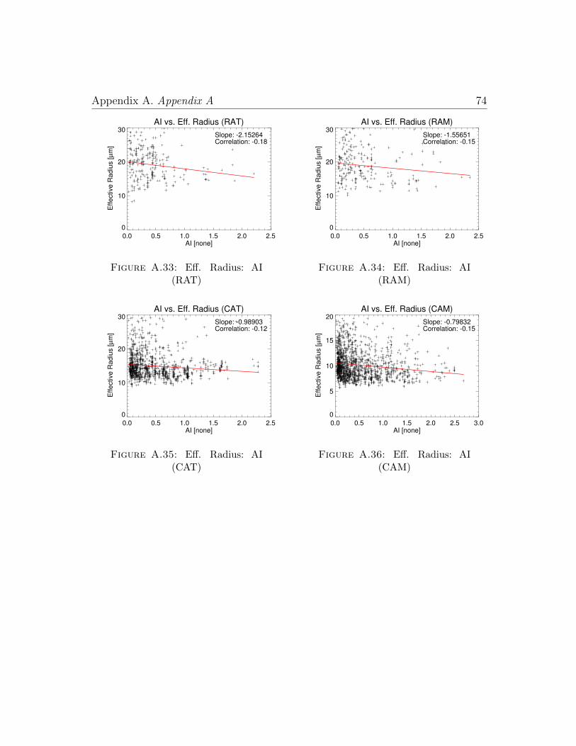
Appendix A. Appendix A 74
AI vs. Eff. Radius (RAT)
0.0 0.5 1.0 1.5 2.0 2.5AI [none]
0
10
20
30
Effective R
adiu
s [
µm
]
Slope: -2.15264Correlation: -0.18
Figure A.33: Eff. Radius: AI(RAT)
AI vs. Eff. Radius (RAM)
0.0 0.5 1.0 1.5 2.0 2.5AI [none]
0
10
20
30
Effective R
adiu
s [
µm
]
Slope: -1.55651Correlation: -0.15
Figure A.34: Eff. Radius: AI(RAM)
AI vs. Eff. Radius (CAT)
0.0 0.5 1.0 1.5 2.0 2.5AI [none]
0
10
20
30
Effective R
adiu
s [
µm
]
Slope: -0.98903Correlation: -0.12
Figure A.35: Eff. Radius: AI(CAT)
AI vs. Eff. Radius (CAM)
0.0 0.5 1.0 1.5 2.0 2.5 3.0AI [none]
0
5
10
15
20E
ffective R
adiu
s [
µm
]Slope: -0.79832Correlation: -0.15
Figure A.36: Eff. Radius: AI(CAM)

Appendix A. Appendix A 75
AI vs. Eff. Radius (CAB)
0.0 0.5 1.0 1.5 2.0 2.5AI [none]
0
2
4
6
8
10
12
Effective R
adiu
s [
µm
]
Slope: -0.20739Correlation: -0.11
Figure A.37: Eff. Radius: AI(CAB)
AOD vs. Eff. Radius (RAT)
0 1 2 3 4 5AOD [none]
0
10
20
30
Effective R
adiu
s [
µm
]
Slope: -1.86884Correlation: -0.17
Figure A.38: Eff. Radius: AOD(RAT)
AOD vs. Eff. Radius (RAM)
0 1 2 3 4 5AOD [none]
0
10
20
30
Effective R
adiu
s [
µm
]
Slope: -1.43290Correlation: -0.15
Figure A.39: Eff. Radius: AOD(RAM)
AOD vs. Eff. Radius (RAB)
0.0 0.5 1.0 1.5 2.0AOD [none]
0
10
20
30
Effective R
adiu
s [
µm
]
Slope: -3.85660Correlation: -0.19
Figure A.40: Eff. Radius: AOD(RAB)
AOD vs. Eff. Radius (CAM)
0 1 2 3 4 5AOD [none]
0
5
10
15
20
Effective R
adiu
s [
µm
]
Slope: -0.57801Correlation: -0.16
Figure A.41: Eff. Radius: AOD(CAM)
AOD vs. Eff. Radius (CAB)
0 1 2 3 4 5AOD [none]
0
2
4
6
8
10
12
Effective R
adiu
s [
µm
]
Slope: -0.18041Correlation: -0.11
Figure A.42: Eff. Radius: AOD(CAB)
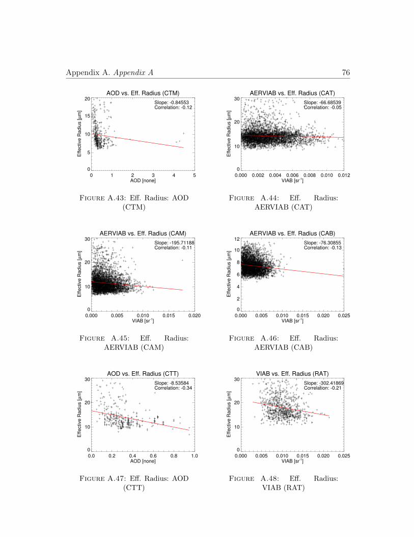
Appendix A. Appendix A 76
AOD vs. Eff. Radius (CTM)
0 1 2 3 4 5AOD [none]
0
5
10
15
20
Effective R
adiu
s [
µm
]
Slope: -0.84553Correlation: -0.12
Figure A.43: Eff. Radius: AOD(CTM)
AERVIAB vs. Eff. Radius (CAT)
0.000 0.002 0.004 0.006 0.008 0.010 0.012VIAB [sr-1]
0
10
20
30
Effective R
adiu
s [
µm
]
Slope: -66.68539Correlation: -0.05
Figure A.44: Eff. Radius:AERVIAB (CAT)
AERVIAB vs. Eff. Radius (CAM)
0.000 0.005 0.010 0.015 0.020VIAB [sr-1]
0
10
20
30
Effective R
adiu
s [
µm
]
Slope: -195.71188Correlation: -0.11
Figure A.45: Eff. Radius:AERVIAB (CAM)
AERVIAB vs. Eff. Radius (CAB)
0.000 0.005 0.010 0.015 0.020 0.025VIAB [sr-1]
0
2
4
6
8
10
12
Effective R
adiu
s [
µm
]
Slope: -76.30855Correlation: -0.13
Figure A.46: Eff. Radius:AERVIAB (CAB)
AOD vs. Eff. Radius (CTT)
0.0 0.2 0.4 0.6 0.8 1.0AOD [none]
0
10
20
30
Effective R
adiu
s [
µm
]
Slope: -8.53584Correlation: -0.34
Figure A.47: Eff. Radius: AOD(CTT)
VIAB vs. Eff. Radius (RAT)
0.000 0.005 0.010 0.015 0.020 0.025VIAB [sr-1]
0
10
20
30
Effective R
adiu
s [
µm
]
Slope: -302.41869Correlation: -0.21
Figure A.48: Eff. Radius:VIAB (RAT)

Appendix A. Appendix A 77
VIAB vs. Eff. Radius (RAM)
0.000 0.005 0.010 0.015 0.020 0.025 0.030VIAB [sr-1]
0
10
20
30
Effective R
adiu
s [
µm
]
Slope: -342.72517Correlation: -0.25
Figure A.49: Eff. Radius:VIAB (RAM)
VIAB vs. Eff. Radius (RAB)
0.000 0.005 0.010 0.015 0.020 0.025VIAB [sr-1]
0
10
20
30
Effective R
adiu
s [
µm
]
Slope: -433.05254Correlation: -0.23
Figure A.50: Eff. Radius:VIAB (RAB)
VIAB vs. Eff. Radius (CAT)
0.00 0.01 0.02 0.03 0.04 0.05VIAB [sr-1]
0
10
20
30
Effective R
adiu
s [
µm
]
Slope: -195.04546Correlation: -0.20
Figure A.51: Eff. Radius:VIAB (CAT)
VIAB vs. Eff. Radius (CAM)
0.00 0.02 0.04 0.06 0.08VIAB [sr-1]
0
10
20
30
Effective R
adiu
s [
µm
]
Slope: -263.15106Correlation: -0.22
Figure A.52: Eff. Radius:VIAB (CAM)
VIAB vs. Eff. Radius (CAB)
0.00 0.02 0.04 0.06 0.08 0.10 0.12VIAB [sr-1]
0
2
4
6
8
10
12
Effective R
adiu
s [
µm
]
Slope: -37.85044Correlation: -0.10
Figure A.53: Eff. Radius:VIAB (CAB)
CLEARAERVIAB vs. Eff. Radius (CTM)
0.000 0.005 0.010 0.015 0.020 0.025 0.030VIAB [sr-1]
0
5
10
15
Effe
ctiv
e R
adiu
s [µ
m]
Slope: 110.34907Correlation: 0.17
Figure A.54: Eff. Radius:CLEARAERVIAB (CTM)

Appendix A. Appendix A 78
CLEARVIAB vs. Eff. Radius (RAB)
0.00 0.02 0.04 0.06 0.08VIAB [sr-1]
0
10
20
30
Effe
ctiv
e R
adiu
s [µ
m]
Slope: -122.53271Correlation: -0.27
Figure A.55: Eff. Radius:CLEARVIAB (RAB)
CLEARVIAB vs. Eff. Radius (CTT)
0.00 0.01 0.02 0.03 0.04 0.05VIAB [sr-1]
0
10
20
30
Effe
ctiv
e R
adiu
s [µ
m]
Slope: -112.16227Correlation: -0.18
Figure A.56: Eff. Radius:CLEARVIAB (CTT)
CLEARTOT vs. Eff. Radius (RAB)
0.00 0.02 0.04 0.06 0.08VIAB [sr-1]
0
10
20
30
Effe
ctiv
e R
adiu
s [µ
m]
Slope: -85.56132Correlation: -0.26
Figure A.57: Eff. Radius:CLEARTOT (RAB)
CLEARTOTAER vs. Eff. Radius (CAT)
0.000 0.005 0.010 0.015 0.020 0.025VIAB [sr-1]
0
10
20
30
Effe
ctiv
e R
adiu
s [µ
m]
Slope: -222.40341Correlation: -0.16
Figure A.58: Eff. Radius:CLEARTOTAER (CAT)
CLEARTOTAER vs. Eff. Radius (CTM)
0.00 0.01 0.02 0.03 0.04VIAB [sr-1]
0
5
10
15
Effe
ctiv
e R
adiu
s [µ
m]
Slope: 74.23521Correlation: 0.18
Figure A.59: Eff. Radius:CLEARTOTAER (CTM)
CLEARLOWAER vs. Eff. Radius (CTT)
0.00 0.01 0.02 0.03 0.04VIAB [sr-1]
0
10
20
30
Effe
ctiv
e R
adiu
s [µ
m]
Slope: 197.68920Correlation: 0.18
Figure A.60: Eff. Radius:CLEARLOWAER (CTT)

Appendix B. Appendix B 79
Appendix B
Probability of Precipitation
Probability of Precipitation-CLEARLOW
0.00 0.05 0.10 0.15 0.20 0.25 0.30LWP [kg m-2]
0
20
40
60
80
100
PoP
[%]
Touch TopTouch Bottom
Figure B.1: Probability of Pre-cipitation: CLEARLOW
Probability of Precipitation-AERVIAB
0.0 0.1 0.2 0.3 0.4LWP [kg m-2]
0
20
40
60
80
100
PoP
[%]
Above TopAbove BottomTouch TopTouch Bottom
Figure B.2: Probability of Pre-cipitation: AERVIAB

Appendix B. Appendix B 80
Probability of Precipitation-VIAB
0.00 0.05 0.10 0.15 0.20 0.25 0.30LWP [kg m-2]
0
20
40
60
80
100
PoP
[%]
Above TopAbove BottomTouch TopTouch Bottom
Figure B.3: Probability of Pre-cipitation: VIAB
Probability of Precipitation-CLEARTOT
0.00 0.05 0.10 0.15 0.20 0.25 0.30LWP [kg m-2]
0
20
40
60
80
100
PoP
[%]
Above TopAbove BottomTouch TopTouch Bottom
Figure B.4: Probability of Pre-cipitation: CLEARTOT
Probability of Precipitation-CLEARTOTAER
0.0 0.1 0.2 0.3LWP [kg m-2]
0
20
40
60
80
100
PoP
[%]
Above TopAbove BottomTouch TopTouch Bottom
Figure B.5: Probability of Pre-cipitation: CLEARTOTAER
Probability of Precipitation-CLEARVIAB
0.00 0.05 0.10 0.15 0.20 0.25 0.30LWP [kg m-2]
0
20
40
60
80
100
PoP
[%]
Above TopAbove BottomTouch TopTouch Bottom
Figure B.6: Probability of Pre-cipitation: CLEARVIAB

Bibliography 81
Bibliography
Ackerman, A., O. Toon, D. Stevens, A. Heymsfield, V. Ramanathan, and E. Wel-
ton, 2000: Reduction of tropical cloudiness by soot. SCIENCE, 288 (5468),
1042–1047, doi:{10.1126/science.288.5468.1042}.
Albrecht, B., 1989: Aerosols, cloud microphysics, and fractional cloudiness. SCI-
ENCE, 245 (4923), 1227–1230, doi:{10.1126/science.245.4923.1227}.
Bennartz, R., 2007: Global assessment of marine boundary layer cloud
droplet number concentration from satellite. Journal of Geophysical Research-
Atmospheres, 112 (D2), doi:ArtnD02201Doi10.1029/2006jd007547, URL
<GotoISI>://000243849400004.
Bennartz, R., J. Fan, J. Rausch, L. R. Leung, and A. K. Heidinger, 2011: Pol-
lution from China increases cloud droplet number, suppresses rain over the
East China Sea. GEOPHYSICAL RESEARCH LETTERS, 38, doi:{10.1029/
2011GL047235}.
Bibliography 82
Breon, F. M. and M. Doutriaux-Boucher, 2005: A comparison of cloud droplet
radii measured from space. Geoscience and Remote Sensing, IEEE Transactions
on, 43 (8), 1796–1805.
Chin, H. N. S., D. J. Rodriguez, R. T. Cederwall, C. C. Chuang, A. S. Grossman,
J. J. Yio, Q. Fu, and M. A. Miller, 2000: A microphysical retrieval scheme for
continental low-level stratiform clouds: Impacts of the subadiabatic character
on microphysical properties and radiation budgets. Monthly Weather Review,
128 (7), 2511–2527, URL <GotoISI>://000166058500008.
Costantino, L. and F. M. Breon, 2013: Aerosol indirect effect on warm clouds
over South-East Atlantic, from co-located MODIS and CALIPSO observations.
ATMOSPHERIC CHEMISTRY AND PHYSICS, 13 (1), 69–88, doi:{10.5194/
acp-13-69-2013}.
Cotton, W. R., G. J. Tripoli, R. M. Rauber, and E. A. Mulvihill, 1986: Numerical-
Simulation of the Effects of Varying Ice Crystal Nucleation Rates and Aggrega-
tion Processes on Orographic Snowfall. Journal of Climate and Applied Meteo-
rology, 25 (11), 1658–1680, URL <GotoISI>://A1986F986900012.
Crutzen, P. J. and M. O. Andreae, 1990: Biomass Burning in the Tropics - Impact
on Atmospheric Chemistry and Biogeochemical Cycles. Science, 250 (4988),
1669–1678, URL <GotoISI>://A1990EN92000032.

Bibliography 83
Eck, T. F., et al., 2013: A seasonal trend of single scattering albedo in southern
African biomass-burning particles: Implications for satellite products and es-
timates of emissions for the world’s largest biomass-burning source. JOURNAL
OF GEOPHYSICAL RESEARCH-ATMOSPHERES, 118 (12), 6414–6432, doi:
{10.1002/jgrd.50500}.
Forster, P. and V. Ramaswamy, 2007: Changes in Atmospheric Constituents and in
Radiative Forcing. Climate Change 2007: The Physical Science Basis, 129–234,
URL <GotoISI>://000292238900004.
Frisch, A. S., C. W. Fairall, and J. B. Snider, 1995: Measurement of Stratus Cloud
and Drizzle Parameters in Astex with a K-Alpha-Band Doppler Radar and a
Microwave Radiometer. Journal of the Atmospheric Sciences, 52 (16), 2788–
2799, URL <GotoISI>://A1995RN65500008.
Haywood, J., S. Osborne, and S. Abel, 2004: The effect of overlying absorbing
aerosol layers on remote sensing retrievals of cloud effective radius and cloud op-
tical depth. QUARTERLY JOURNAL OF THE ROYAL METEOROLOGICAL
SOCIETY, 130 (598, A), 779–800, doi:{10.1256/qj.03.100}.
Ignatov, A., et al., 2005: Two MODIS aerosol products over ocean on the Terra and
Aqua CERES SSF datasets. JOURNAL OF THE ATMOSPHERIC SCIENCES,
62 (4), 1008–1031, doi:{10.1175/JAS3383.1}.

Bibliography 84
Jacobson, M. Z., Y. J. Kaufman, and Y. Rudich, 2007: Examining feedbacks of
aerosols to urban climate with a model that treats 3-D clouds with aerosol
inclusions. Journal of Geophysical Research-Atmospheres, 112 (D24), doi:
ArtnD24205Doi10.1029/2007jd008922, URL <GotoISI>://000252013700013.
Jiang, H. L., G. Feingold, and W. R. Cotton, 2002: Simulations of aerosol-
cloud-dynamical feedbacks resulting from entrainment of aerosol into the ma-
rine boundary layer during the Atlantic Stratocumulus Transition Experiment.
Journal of Geophysical Research-Atmospheres, 107 (D24), doi:Artn4813Doi10.
1029/2001jd001502, URL <GotoISI>://000181262000008.
Jonas, P., 1996: Turbulence and cloud microphysics. ATMOSPHERIC RE-
SEARCH, 40 (2-4), 283–306, doi:{10.1016/0169-8095(95)00035-6}.
Kacenelenbogen, M., et al., 2014: An evaluation of caliop/calipso’s aerosol-above-
cloud detection and retrieval capability over north america. Journal of Geophysi-
cal Research: Atmospheres, 119 (1), 230–244, doi:10.1002/2013JD020178, URL
http://dx.doi.org/10.1002/2013JD020178.
Kaufman, Y. J., I. Koren, L. A. Remer, D. Rosenfeld, and Y. Rudich, 2005: The
effect of smoke, dust, and pollution aerosol on shallow cloud development over the
Atlantic Ocean. Proceedings of the National Academy of Sciences of the United
States of America, 102 (32), 11 207–11 212, doi:Doi10.1073/Pnas.0505191102,
URL <GotoISI>://000231253400017.
Bibliography 85
Kim, M.-H., S.-W. Kim, S.-C. Yoon, and A. H. Omar, 2013: Comparison of aerosol
optical depth between caliop and modis-aqua for caliop aerosol subtypes over the
ocean. Journal of Geophysical Research: Atmospheres, 118 (23), 13,241–13,252,
doi:10.1002/2013JD019527, URL http://dx.doi.org/10.1002/2013JD019527.
Koren, I., L. A. Remer, Y. J. Kaufman, Y. Rudich, and J. V. Martins, 2007: On
the twilight zone between clouds and aerosols. GEOPHYSICAL RESEARCH
LETTERS, 34 (8), doi:{10.1029/2007GL029253}.
L’Ecuyer, T. S., W. Berg, J. Haynes, M. Lebsock, and T. Takemura, 2009:
Global observations of aerosol impacts on precipitation occurrence in warm
maritime clouds. Journal of Geophysical Research-Atmospheres, 114, doi:
ArtnD09211Doi10.1029/2008jd011273, URL <GotoISI>://000265930400005.
Liu, Y. G., B. Geerts, M. Miller, P. Daum, and R. McGraw, 2008:
Threshold radar reflectivity for drizzling clouds. Geophysical Re-
search Letters, 35 (3), doi:ArtnL03807Doi10.1029/2007gl031201, URL
<GotoISI>://000253063700001http://www.agu.org/journals/gl/gl0803/
2007GL031201/2007GL031201.pdf.
Loeb, N. and N. Manalo-Smith, 2005: Top-of-atmosphere direct radiative effect
of aerosols over global oceans from merged CERES and MODIS observations.
JOURNAL OF CLIMATE, 18 (17), 3506–3526, doi:{10.1175/JCLI3504.1}.

Bibliography 86
Loeb, N. G. and G. L. Schuster, 2008: An observational study of the relationship
between cloud, aerosol and meteorology in broken low-level cloud conditions.
JOURNAL OF GEOPHYSICAL RESEARCH-ATMOSPHERES, 113 (D14),
doi:{10.1029/2007JD009763}.
Lu, M. L. and J. H. Seinfeld, 2005: Study of the aerosol indirect effect by large-
eddy simulation of marine stratocumulus. Journal of the Atmospheric Sciences,
62 (11), 3909–3932, URL <GotoISI>://000233460600004.
Marchand, R., G. G. Mace, T. Ackerman, and G. Stephens, 2008: Hydrom-
eteor Detection Using Cloudsat—An Earth-Orbiting 94-GHz Cloud Radar.
Journal of Atmospheric and Oceanic Technology, 25, 519–533, doi:10.1175/
2007JTECHA1006.1.
Matheson, M. A., J. A. Coakley, Jr., and W. R. Tahnk, 2006: Multiyear Ad-
vanced Very High Resolution Radiometer observations of summertime stra-
tocumulus collocated with aerosols in the northeastern Atlantic. JOURNAL
OF GEOPHYSICAL RESEARCH-ATMOSPHERES, 111 (D15), doi:{10.1029/
2005JD006890}.
Nakajima, T. and M. King, 1990: Determination of the optical-thickness and
effective particle radius of clouds from reflected solar-radiation measurements
.1. theory. journal of the atmospheric sciences, 47 (15), 1878–1893, doi:
{10.1175/1520-0469(1990)047〈1878:DOTOTA〉2.0.CO;2}.

Bibliography 87
Omar, A. H., et al., 2009: The CALIPSO Automated Aerosol Classification
and Lidar Ratio Selection Algorithm. Journal of Atmospheric and Oceanic
Technology, 26 (10), 1994–2014, doi:10.1175/2009JTECHA1231.1, URL http:
//dx.doi.org/10.1175/2009JTECHA1231.1.
Painemal, D. and P. Zuidema, 2011: Assessment of MODIS cloud effective radius
and optical thickness retrievals over the Southeast Pacific with VOCALS-REx
in situ measurements. Journal of Geophysical Research-Atmospheres, 116, doi:
ArtnD24206Doi10.1029/2011jd016155, URL <GotoISI>://000298747600001.
Pawlowska, H. and J. L. Brenguier, 2003: An observational study of drizzle for-
mation in stratocumulus clouds for general circulation model (GCM) param-
eterizations. Journal of Geophysical Research-Atmospheres, 108 (D15), doi:
Artn8630Doi10.1029/2002jd002679, URL <GotoISI>://000184805900007.
Pawlowska, H., J. L. Brenguier, and L. Schuller, 1999: Microphysical and ra-
diative properties of stratocumulus. Physics and Chemistry of the Earth Part
B-Hydrology Oceans and Atmosphere, 24 (8), 927–932, URL <GotoISI>://
000083562600009.
Penner, J. E., S. Y. Zhang, and C. C. Chuang, 2003: Soot and smoke
aerosol may not warm climate. Journal of Geophysical Research-
Atmospheres, 108 (D21), doi:Artn4657Doi10.1029/2003jd003409, URL
Bibliography 88
<GotoISI>://000186396400001http://www.agu.org/journals/jd/jd0321/
2003JD003409/2003JD003409.pdf.
Petters, J. L., H. Jiang, G. Feingold, D. L. Rossiter, D. Khelif, L. C. Sloan,
and P. Y. Chuang, 2013: A comparative study of the response of modeled
non-drizzling stratocumulus to meteorological and aerosol perturbations. AT-
MOSPHERIC CHEMISTRY AND PHYSICS, 13 (5), 2507–2529, doi:{10.5194/
acp-13-2507-2013}.
Powell, K. and M. Vaughan, 2013: Cloud-aerosol lidar infrared pathfinder satellite
observations: Data management system-data products catalog. URL http://
www-calipso.larc.nasa.gov/products/CALIPSO_DPC_Rev3x6.pdf.
Quaas, J., O. Boucher, N. Bellouin, and S. Kinne, 2008: Satellite-based estimate of
the direct and indirect aerosol climate forcing. JOURNAL OF GEOPHYSICAL
RESEARCH-ATMOSPHERES, 113 (D5), doi:{10.1029/2007JD008962}.
Roberts, G., M. J. Wooster, and E. Lagoudakis, 2009: Annual and diurnal african
biomass burning temporal dynamics. Biogeosciences, 6 (5), 849–866, URL
<GotoISI>://000266556300009.
Rosenfeld, D., 2000: Suppression of rain and snow by urban and indus-
trial air pollution. Science, 287 (5459), 1793–1796, URL <GotoISI>:
//000085775300034http://www.sciencemag.org/content/287/5459/1793.
full.pdf.

Bibliography 89
Rosenfeld, D., H. Wang, and P. J. Rasch, 2012: The roles of cloud drop effec-
tive radius and LWP in determining rain properties in marine stratocumulus.
GEOPHYSICAL RESEARCH LETTERS, 39, doi:{10.1029/2012GL052028}.
Sekiguchi, M., T. Nakajima, K. Suzuki, K. Kawamoto, A. Higurashi, D. Rosen-
feld, I. Sano, and S. Mukai, 2003: A study of the direct and indirect effects
of aerosols using global satellite data sets of aerosol and cloud parameters.
JOURNAL OF GEOPHYSICAL RESEARCH-ATMOSPHERES, 108 (D22),
doi:{10.1029/2002JD003359}.
Tanre, D., Y. Kaufman, M. Herman, and S. Mattoo, 1997: Remote sensing of
aerosol properties over oceans using the MODIS/EOS spectral radiances. JOUR-
NAL OF GEOPHYSICAL RESEARCH-ATMOSPHERES, 102 (D14), 16 971–
16 988, doi:{10.1029/96JD03437}.
Twohy, C. H., J. A. Coakley, Jr., and W. R. Tahnk, 2009: Effect of changes in rela-
tive humidity on aerosol scattering near clouds. JOURNAL OF GEOPHYSICAL
RESEARCH-ATMOSPHERES, 114, doi:{10.1029/2008JD010991}.
Twomey, S., 1974: Pollution and Planetary Albedo. Atmospheric Environment,
8 (12), 1251–1256, URL <GotoISI>://A1974U971800003.
Twomey, S., 1977: Influence of pollution on shortwave albedo of clouds. JOUR-
NAL OF THE ATMOSPHERIC SCIENCES, 34 (7), 1149–1152, doi:{10.1175/
1520-0469(1977)034〈1149:TIOPOT〉2.0.CO;2}.

Bibliography 90
Twomey, S. and K. Seton, 1980: Inferences of gross microphysical properties of
clouds from spectral reflectance measurements. journal of the atmospheric sci-
ences, 37 (5), 1065–1069, doi:{10.1175/1520-0469(1980)037〈1065:IOGMPO〉2.
0.CO;2}.
Varnai, T. and A. Marshak, 2009: Modis observations of enhanced clear sky
reflectance near clouds. Geophysical Research Letters, 36 (6), n/a–n/a, doi:
10.1029/2008GL037089, URL http://dx.doi.org/10.1029/2008GL037089.
Wang, J. Y. and B. Geerts, 2003: Identifying drizzle within marine stratus with
W-band radar reflectivity. Atmospheric Research, 69 (1-2), 1–27, doi:Doi10.
1016/J.Atmosres.2003.08.001, URL <GotoISI>://000187154900001http:
//ac.els-cdn.com/S0169809503001133/1-s2.0-S0169809503001133-main.
pdf?_tid=9d6d1e0e4b5da6b453562e2fbf39d4eb&acdnat=1335282270_
5f98e95b4fa848c107a5827d4f70ce17.
Wen, G., A. Marshak, R. F. Cahalan, L. A. Remer, and R. G. Kleidman, 2007:
3-d aerosol-cloud radiative interaction observed in collocated modis and aster
images of cumulus cloud fields. Journal of Geophysical Research: Atmospheres,
112 (D13), n/a–n/a, doi:10.1029/2006JD008267, URL http://dx.doi.org/
10.1029/2006JD008267.
Winker, D. M., M. A. Vaughan, A. Omar, Y. Hu, K. A. Powell, Z. Liu, W. H.
Hunt, and S. A. Young, 2009: Overview of the CALIPSO Mission and CALIOP

Bibliography 91
Data Processing Algorithms. JOURNAL OF ATMOSPHERIC AND OCEANIC
TECHNOLOGY, 26 (11), 2310–2323, doi:{10.1175/2009JTECHA1281.1}.
Wu, L., H. Su, and J. H. Jiang, 2013: Regional simulation of aerosol im-
pacts on precipitation during the East Asian summer monsoon. JOURNAL
OF GEOPHYSICAL RESEARCH-ATMOSPHERES, 118 (12), 6454–6467, doi:
{10.1002/jgrd.50527}.
Zhang, J., J. S. Reid, and B. N. Holben, 2005: An analysis of potential cloud
artifacts in modis over ocean aerosol optical thickness products. Geophysical
Research Letters, 32 (15), n/a–n/a, doi:10.1029/2005GL023254, URL http:
//dx.doi.org/10.1029/2005GL023254.