Objectives/key terms - OpenStudyassets.openstudy.com/updates/attachments/4f92f31de4… · ·...

Objectives/key terms

PURCHASING POWERPARITY

20

• Law of One Price

• Purchasing power parity (PPP)

• Real effective exchange rate

• Differentiated goods

• Non-traded goods

• PPP corrections

• Absolute and relative version

• Real (bilateral) exchange rate

• Transaction costs

• Fixed investment and thresholds

• Harrod–Balassa–Samuelson effect

• Endogenous and exogenous

We discuss absolute and relative versions of the Law of One Price (for individual goods)

and purchasing power parity (PPP, for price indices). There can be substantial short-run

deviations from PPP, but in the long run relative PPP holds remarkably well because

fundamentals and arbitrage are dominant long-run economic forces.

20-Marr-Chap20.qxd 31/10/06 10:41 AM Page 426

20.1 IntroductionAccording to the Law of One Price identical goods should (under certain conditions) sell forthe same price in two different countries at the same time. It is the foundation for purchasingpower parity (PPP) theory, which relates exhange rates and price levels. The absolute PPPexchange rate equates the national price levels in two countries if expressed in a commoncurrency at that rate, so that the purchasing power of one unit of a currency would be thesame in the two countries. Relative PPP focuses on changes in the price levels andthe exchange rate, rather than the level. Although the term purchasing power parity wasapparently first used by Cassel (1918), the ideas underlying PPP have a history dating back atleast to scholars at the University of Salamanca in the fifteenth and sixteenth centuries; seeOfficer (1982). As we will see, long-run relative PPP holds remarkably well, even though therecan be substantial short-run deviations from relative PPP. Many structural models that seek toexplain exchange rates and exchange rate behaviour are based on this presumption, leadingRogoff (1992) to conclude that most international economists ‘instinctively believe in somevariant of purchasing power parity as an anchor for long-run real exchange rates’.

20.2 The Law of One Price and Purchasing Power ParitySuppose that the exact same product, say a computer chip, is freely traded in two differentcountries, say America (sub-index A) and Britain (sub-index B). Suppose, furthermore, thatthere are no transportation costs, no tariffs, no fixed investments necessary for arbitrage, andno other impediments to trade flows between these two countries of any type whatsoever.Should not, under those conditions, the (appropriately measured) price of the computer chipin Britain be the same as in America? According to the Law of One Price, it should. Obviously,we have made a range of assumptions before we came to the conclusion that arbitrage shouldensure that the Law of One Price holds. Any violation of these conditions can, in principle,cause a violation of this law. We discuss these issues in the second part of this chapter.

P U R C H A S I N G P OW E R PA R I T Y 427

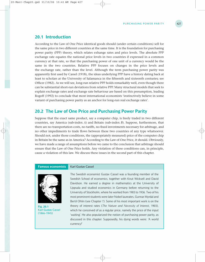
Famous economists Karl Gustav Cassel

The Swedish economist Gustav Cassel was a founding member of the

Swedish School of economics, together with Knut Wicksell and David

Davidson. He earned a degree in mathematics at the University of

Uppsala and studied economics in Germany before returning to the

University of Stockholm, where he worked from 1903 to 1936. Two of his

most prominent students were later Nobel laureates, Gunnar Myrdal and

Bertil Ohlin (see Chapter 7). Some of his most important work is on the

theory of interest rates (The Nature and Necessity of Interest, 1903),

which he conceived of as a regular price, namely the price of the input

‘waiting’. He also popularized the notion of purchasing power parity, as

discussed in this chapter. Supposedly, his dying words were: ‘A world

currency!’

Fig. 20.1Karl Gustav Cassel(1866–1945)


There are, actually, different versions of the Law of One Price. There is a strong absoluteversion and a weaker relative version. Both can be applied to individual products and to priceindices. Let’s start with the strongest version of all. Suppose we have a large number N ofindividual products consumed and produced in America and Britain (computer chips, flour,cars, movies, etc.). We let the sub-index i denote the type of product (so i ranges from 1 to N )and the sub-index t denote time (which could, for example, be quarters, months, or days).Then the absolute version of the Law of One Price for each individual good i implies:

(20.1)

where is the price of good i in America at time t (in dollars), is the price of the samegood in Britain at the same time (in pounds sterling), and is the nominal exchange rate ofthe US dollar (the price in pounds sterling for purchasing one dollar).

Equation (20.1) imposes a restriction on the price levels of the same good in differentcountries. Instead, the relative version of the Law of One Price imposes a restriction on thechanges in these price levels, more specifically:

(20.1�)

In essence, the relative version argues that the deviation, if any, between the prices of somegood in the two countries in one time period also holds in the next period. The relativeversion of the Law of One Price is weaker than the absolute version, simply because equation(20.1) implies equation (20.1�), but not vice versa. That is, if there is a constant deviation fromthe Law of One Price, the relative version holds while the absolute version does not.

To get from the Law of One Price to purchasing power parity (henceforth PPP), we have togo from the microeconomic to the macroeconomic level and look at price indices. Virtuallyall countries publish several types of price indices, such as the consumer price index, theproducer price index, the GDP deflator, etc. All of these are constructed in different ways,emphasize different aspects of the economy and can be used for PPP comparisons; see alsoBox 20.2. The exposition below focuses on the consumer price index (CPI). The CPI is usuallyconstructed as a weighted average of the prices of individual (groups of) products, with theweights representing the share of income spent by households on a particular product insome reference year. Let be the weight of product i and let denote America’s price indexin period t, given by

(20.2)

Now suppose that Britain’s price index is constructed identically (this need not be thecase, which is a potential cause for PPP deviations, see Sections 20.4 and 20.5). If the absoluteversion of the Law of One Price (equation 20.1) holds for individual products, this meansthere is a clear relationship between the exchange rate and the price indices in Britain andAmerica:

(20.3)

where the second term from the left is simply the definition of Britain’s price index, the thirdterm follows from the absolute Law of One Price for individual products, the fourth term takes

PB,t � �N

i�1�i PBi,t � �

N

i�1�i (St PAi,t) � St �

N

i�1�i PAi,t � St PA, t ,

PB,t

PA,t � �N

i�1�i PAi,t, with �i �0, �

N

i�1�i � 1

PA,t�i

St�1 PAi,t�1

PBi,t�1�

St PAi,t

PBi,t

, i � 1, . . . , N.

St

PBi,tPAi,t

PBi,t � St PAi,t , i � 1, . . . , N.

I N T E R N AT I O N A L M O N E Y : M O N E Y B A S I C S428


the (common) exchange rate out of the summation sign, and the fifth term follows from thedefinition of America’s price index. The first and last terms of equation (20.3) can be moreconveniently written in logarithmic form. As this is the case more generally in the monetaryparts of this book, we henceforth agree to the following:

Convention: a lower-case letter x of a variable X in general denotes its natural logarithm, that is x� ln (X). So, for example, , , etc.

Using this convention, a slight re-arrangement of equation (20.3) gives us the absoluteversion of PPP in logarithmic terms; see equation (20.4). Writing the latter in time differencesgives us the relative version of PPP; see equation (20.4�).

(20.4)

(20.4�)

The relative version of PPP (eq. 20.4�) can be derived either from the absolute version of PPP(eq. 20.4) or from the relative version of the Law of One Price (eq. 20.1�).1 Both of these can,in turn, be derived from the absolute version of the Law of One Price. Figure 20.2schematically summarizes the strongness of these ‘laws’ and their relationships. The absoluteversion of the Law of One Price for individual goods is the strongest condition and, undersome qualifications, implies all other versions without being implied by any of them.Similarly, the relative version of PPP is the weakest of all assumptions: it is implied by all otherversions and does not imply any of them.

20.3 Prices and exchange ratesIs there an empirical relationship between exchange rates and price indices, as suggested bythe PPP conditions in Section 20.2? There certainly is! A very simple, but quite convincing,demonstration of this relationship is based on the (weakest) relative PPP version (eq. 20.4�),as illustrated in Figure 20.3. As we will argue below, the PPP relationship is actually a long-run

(st�1 � st) � (pB,t�1 � pB,t) � (pA,t�1 � pA,t)

st � pB,t � pA,t

pA,t � ln (PA,t)st � ln (St)


Absolute Law of One Price, individual goods

Relative Law of One Price, individual goods

Implies

ImpliesAbsolute PPP = absolute Law of

One Price forprice index

Relative PPP = relative Law of

One Price for price index

Implies Implies

Figure 20.2 Different versions of the Law of One Price and PPP*

Note: * Some qualifications for the implication arrows may apply; see the main text for details.

20-Marr-Chap20.qxd 31/10/06 10:41 AM 29

relationship, with substantial deviations from PPP ‘equilibrium’ in the short run. To findsupporting evidence of relative PPP, we therefore have to look at a long enough time periodto ensure that the deviations between developments in price indices in two differentcountries are big enough, and the associated economic arbitrage forces strong enough, toallow for these differences to have an impact on the exchange rate. Using World Bank data,we can analyse a time period of 41 years. At this stage, we are not interested in the details ofthe developments over time, just in the extremes, that is the first year of observation (1960)and the last year of observation (2001). We will use the USA as benchmark country. Underthose circumstances, the (logarithmic) relative PPP equation (20.4’) translates into:

(20.5)

where s is the US dollar exchange rate in foreign currency and pcj is the consumer price indexfor the 55 countries for which both exchange rates and price indices were available.Figure 20.3 depicts the left-hand side of equation (20.5) on the horizontal axis and the right-hand side on the vertical axis for 55 data points. They are nearly all on a straight line throughthe origin with a 45-degree slope (also depicted in the figure), as would be predicted by equa-tion (20.5), providing visual support for the relative PPP hypothesis. The largest deviationsfrom the 45-degree line are some (mostly Latin American) countries at the upper-right handof the diagram which have had very high inflation rates relative to the USA and concomitanthigh increases in the US dollar exchange rate.

(20.5�)

Equation (20.5’) reports the econometric estimate of equation (20.5) based on the empiricalobservations depicted in Figure 20.3. See Box 20.1 for an explanation of this procedure. The

s2001 � s1960 � 0.235(0.0875)

� 0.993(0.0174)

� [(pcj,2001 � pcj,1960) � (pUS,2001 � pUS,1960)]

s2001 � s1960 � (p cj,2001 � pcj,1960) � (pUS,2001 � p US,1960); cj � 1, . . . , 55,


–3

0

3

6

9

12

15

18

21

US $ exchange rates and consumer prices, 1960–2001

–3 0 3 6 9 12 15 18 21

s20012s1960

(pcj,2

0012

p cj,1

960)

2(p

US,

2001

2p U

S,19

60)

Sudan

Uruguay

Peru

Bolivia

Figure 20.3 Exchange rates and prices, 1960–2001

Note: Calculations based on World Bank Development Indicators CD-ROM 2003; 55observations; the line has a 45-degree slope; see the main text for details.



Box 20.1 Basic econometrics

When we are developing different theories to try to better understand various economic phenomena,we often assume that the relationships between the economic variables we are analysing are exact.In principle, our theories should lead to results, that is, propositions or predictions that should holdempirically if the theory is true. If we gather economic data to test if the theoretical implications doindeed hold in reality, we need a method to determine if a theory is refuted or not. This is the workof econometricians. In practice, things are, as usual, not quite that simple for four main reasons.

1. We must recast the theory in a manner suitable for empirical evaluation and testing. This meanswe have to acknowledge the fact that the relationships between the economic variables of ourtheories are not exact due to simplifications and disturbances. There may, therefore, be devia-tions from the exact relationships that we can attribute to other phenomena, such as measure-ment errors or the weather, which do not immediately refute the theory. The point is, of course,that these deviations should not be ‘too large’.

2. It can be very complicated, even after overcoming the first problem, to actually test the implicationsof a theory for technical or econometric reasons. Numerous examples can be given of the manyhurdles econometricians sometimes have to take and traps to avoid, before they can devise anadequate test of what may at first look like a simple implication of a theory. Section 20.6 discussessome of these problems when testing for purchasing power parity.

3. It can be virtually impossible, even after overcoming the first and second problems, to pinpointthe nature of an observed friction between theory and empirics. Remember that our theories areusually based on a range of assumptions. In many cases, economic theorists may be convinced bythe arguments of econometricians that an implication of a theory does not hold in practice, butdisagree strongly on the particular assumption on which the theory was based which caused thisfriction. It can take several decades of scientific research, involving the development of new theo-ries and new tests, etc., before some, if any, consensus on the nature of the problem is reached.

4. Even if an empirical test confirms our theory, this does not necessarily prove it. Maybe someother theory can also explain the observations; we are never really sure.

The remainder of this box focuses on the simplest version of the first problem. Suppose we have aneconomic theory that predicts a linear relationship between the economic variables y and x:

. Since all theories are simplifications of reality (which is what makes it theory), there isalways a range of phenomena that might influence the actual relationship between the variables yand x. There can be other, more complicated, economic forces not modelled in the theory thatcould affect the relationship; there can be forces outside of economics (such as the weather, vol-canic eruptions, or political changes) that could affect it; there can be errors in measurement, etc.This leads us to posit that the observed relationship is as follows:

(20.6) yt � a + bxt + ut,

where the sub-index t denotes different observations (for example different time periods or differentcountries) and the variable denotes the deviation between the structural linear part of an obser-vation and the actual value of the observation. This deviation should not be ‘too large’, so

ut

y � a � bx

g



g when we average it over many observations its value should be zero (it is, for example,normally distributed with mean 0 and variance ).

An econometrician is, of course, not given the ‘true’ parameters a and b of the structural linearequation (although there may be ‘implied’ theoretical values, as discussed in this chapter). Instead,she is given a number of observations, that is joint pairs of the economic variables x and y.These are depicted as the dots (or balls) in Figure 20.4. Her task is then to find the best line to fitthese empirical observations, that is estimate an intercept, say , and a slope, say , to minimize the(quadratic) distance from the observations to the line. We are not concerned with how this is donehere. Instead, we briefly discuss how hypotheses can be tested using this procedure.

Figure 20.4 was artificially constructed based on a ‘true’ model with intercept 2 and slope 1( ) by adding (normally distributed) disturbances using a random number gener-ator. Since the econometrician is only given the observations and not the true parameters, she triesto estimate these ( and ) based on the observations. The terminology is to ‘run a regression’,where y is the endogenous variable (the variable to be explained) and x is the exogenous variable(the explanatory variable). She finds:

(20.7)

The numbers in parentheses in equation (20.7) are estimated standard errors of the estimatedcoefficients, see below. Instead of the true parameter 2, the econometrician therefore estimates theintercept to be 2.776, and instead of the true parameter 1, she estimates the slope to be 0.872. Well,we do not expect her to find the exact parameters, but how far off is she, is this within acceptablelimits, and how good is the ‘fit’ of the estimated line? To start with the last point, it is clear that thefit is better the closer the observations are to the estimated line. A popular measure for this fit is the

y � 2.776(0.4730)

� 0.872(0.0744)

·x

ba

uta � 2, b � 1

ba

(xt,yt)

�2

0

5

10

0 5 10Variable x

Var

iabl

e y

Objective: draw straight line such that the sum of distance from observations (dots) to straight line is 'minimized'

observations

Figure 20.4 Basic econometrics: observations and lines

g


estimated standard errors are denoted in parentheses immediately below the estimatedcoefficients. The overall goodness-of-fit is quite high, as 98.4 per cent of the variance isexplained by the regression (R2 � 0.984). Some simple hypotheses tests would show that theestimated slope coefficient does not differ significantly from one (as would be implied byrelative PPP theory) and that the estimated intercept is (just) significant (in contrast to thistheory).2 A more thorough discussion of these issues is deferred to Section 20.6.

20.4 Real effective exchange ratesSection 20.2 derived the nominal exchange rate between two countries consistent withabsolute or relative PPP; see equations (20.4) and (20.4�). On that basis, we can now define (inlogarithmic terms) the real (bilateral) exchange rate, say qt, as the difference between the nom-inal effective exchange rate and the price indices of the two countries:

(20.8) .

This real exchange rate then provides a measure of the deviation from PPP between the twocountries. We can, of course, also calculate the relative counterpart of the bilateral realexchange rate by taking the first difference of equation (20.8). In both cases, developments inthe nominal exchange rate are corrected for developments in the price levels of the two coun-tries, implying that the real exchange rate is a measure of the evolution of one country’scompetitiveness relative to another country. More specifically, if the real exchange rate inequation (20.8) increases, this implies that the higher price of the US dollar ( ) is onlypartially offset by differences in price developments between Britain and America ( ),so that America has become less competitive compared to Britain.

In practice, countries are more interested in the general development of their competitiveposition, not just relative to one country in particular. The real effective exchange rate doesjust that, by calculating a weighted average of the bilateral real exchange rates (see also

pB,t � pA,t

st

qt �

st � (pB,t � pA,t)


g share of the variance of the variable y explained by the estimated line, the so-called . In thiscase, 83.1 per cent of the variance is explained by the regression ( ). In general, the higherR2, the better the fit. It should be noted, however, that the share of the variance that can beexplained differs widely per application, with some areas of economics where researchers are happyif they can explain 20 per cent of the variance and others where less than 90 per cent is consideredbad. In this respect, the standard errors reported in equation (20.8) are more useful as they indicatethe reliability of the estimated coefficients. They can be used for hypothesis testing. Based on the so-called t-distribution, we can calculate the probability that the true parameter has a particular value,given the observations on the pairs available to us and the associated regression line. As arough rule of thumb: hypotheses within two standard deviations away from the estimatedcoefficient are accepted (in this case: slope in between 0.7232 and 1.0208 and intercept in between1.830 and 3.722). Alternatively, the rule of thumb implies that an absolute t-value larger than 2denotes a ‘significant’ parameter as the estimated coefficient differs from the hypothesis ‘equal tozero’ by more than two standard deviations.

(xt,yt)

R2 � 0.831R2


Section 20.5). It plays an important role in policy analysis as an indicator of the competitivenessof domestic relative to foreign goods and the demand for domestic and foreign currencyassets. As the real effective exchange rate is an index, the focus is on changes of the indexrelative to some base year; that is, the policy focus is on relative and not absolute PPP.

The Federal Reserve has changed its weighting procedure from the earlier used share of totaltrade to a third-market competitiveness index, based on the share of a foreign country’s goodsin all markets that are important to US producers (see Box 20.2 for the European CentralBank’s method in this respect). Figure 20.5 illustrates the difference between these twoprocedures for the six largest trading partners of the USA. Note that for the competitivenessindex: (i) the developments tend to be more stable over time (see e.g. Japan), (ii) theimportance of neighbouring states (Canada and Mexico) is reduced, as is (to a smaller extent)the importance of Japan, and (iii) the importance of Europe is increased. The developments


(a)

(b)

USA: trade weights, percent of total

0

5

10

15

20

1980 1985 1990 1995 year

Euro area

UK

China

Japan

Canada

Mexico

Japan

USA: third-market competitiveness weights

0

5

10

15

20

25

1980 1985 1990 1995 year

Euro area

UK

China

Japan

Canada Mexico

20001975

20001975

Figure 20.5 US dollar: trade weights (top six) and competitiveness weights

Data source: www.federalreserve.gov


for China are similar using either trade weights or competitiveness weights, rising from lessthan 2 per cent in 1980 to about 10 per cent in 2004.

Figure 20.6 shows the evolution of the real and nominal effective exchange rates for theUSA in the period 1975–September 2004. As panel (a) makes clear, there is a big difference inthe development of the real versus the nominal effective exchange rates for the broad rangeof currencies. There is, in particular, no consistent increase in the real value of the US dollar.The developments for the nominal and real exchange rates using the major foreign currenciesas a benchmark are much more similar; see panel (b). As already explained in Section 19.5,this difference is caused by the inclusion of high-inflation countries in the broad index, com-pared to the absence of such countries in the major index. As panel (c) illustrates, there is littledeviation in the developments of the real index for the major and broad index.


(a) (b)

(c)

USA: effective exchange rates, broad

0

30

60

90

120

150

30

60

90

120

1980 1985 1990 1995 2000

NominalReal

USA: effective exchange rates, major

1980 1985 1990 1995 2000

Real

Nominal

US dollar: real effective exchange rates, index (monthly)

75

85

95

105

115

125

135

1985 1995

Major currencies

Broad currencies

20051975 20051975

150

0

20051975

Figure 20.6 US dollar: real effective exchange rates

Note: See Chapter 19 for ‘major’ and ‘broad’ index.

Data source: www.federalreserve.gov


Can we infer from Figure 20.6 whether or not PPP holds empirically? Well, yes and no.Ignoring changes in the underlying weights, if relative PPP were to hold for every time periodand for all countries, the real effective exchange rate would have to be a horizontal line. Ifabsolute PPP holds, the level of this line would be determined. Taking the broad index in


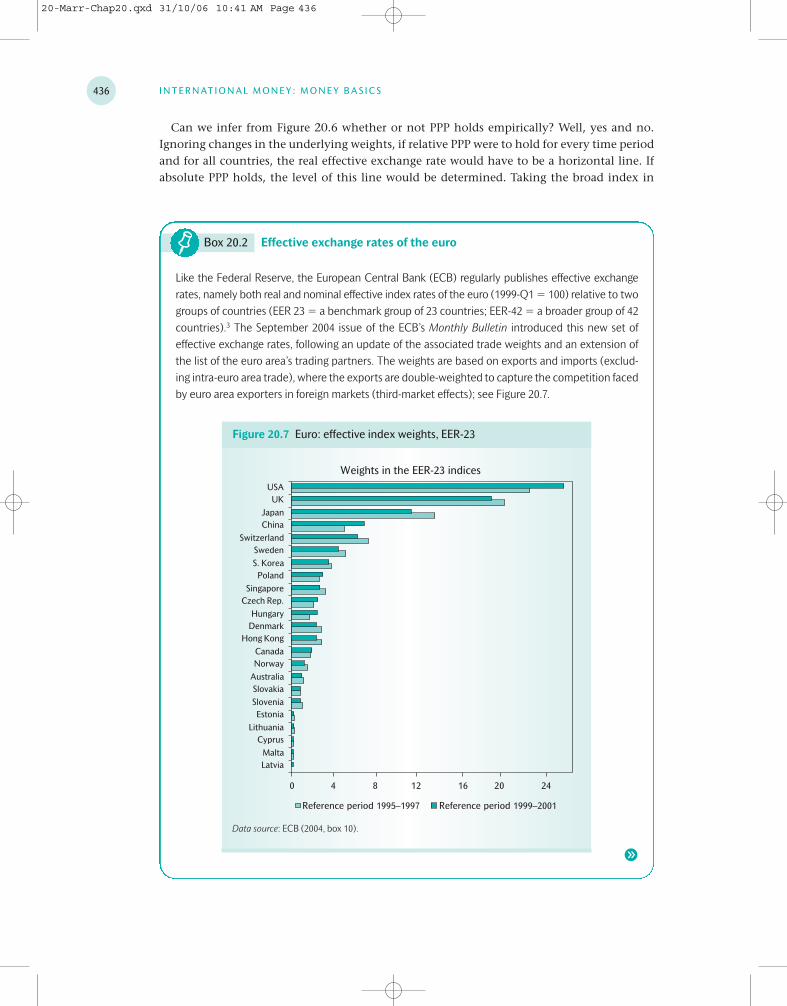
Box 20.2 Effective exchange rates of the euro

Like the Federal Reserve, the European Central Bank (ECB) regularly publishes effective exchangerates, namely both real and nominal effective index rates of the euro (1999-Q1 � 100) relative to twogroups of countries (EER 23 � a benchmark group of 23 countries; EER-42 � a broader group of 42countries).3 The September 2004 issue of the ECB’s Monthly Bulletin introduced this new set ofeffective exchange rates, following an update of the associated trade weights and an extension ofthe list of the euro area’s trading partners. The weights are based on exports and imports (exclud-ing intra-euro area trade), where the exports are double-weighted to capture the competition facedby euro area exporters in foreign markets (third-market effects); see Figure 20.7.

Weights in the EER-23 indices

0 4 8 12 16 20 24

LatviaMalta

CyprusLithuania

EstoniaSloveniaSlovakia

AustraliaNorwayCanada

Hong KongDenmarkHungary

Czech Rep.Singapore

PolandS. KoreaSweden

SwitzerlandChinaJapan

UKUSA

Reference period 1995–1997 Reference period 1999–2001

Figure 20.7 Euro: effective index weights, EER-23

Data source: ECB (2004, box 10).

g


g

panel (a) as our point of reference, the US real effective exchange rate clearly is not ahorizontal line. Relative PPP therefore does not hold for all time periods. There is not,however, a consistent upward or downward movement. Instead, compared to a baseline ofroughly 90 points, there are two large upward deviations (as indicated in panel (a)) namelyin the period 1981–88 (with a peak in March 1985) and in the period 1997–2004 (with a peakin February 2002). Both these periods and their relationships with economic policy will bediscussed in forthcoming chapters. For now, it suffices to note that on the basis of the USexperience, short-run relative PPP does not hold. Indeed, there can be large and prolongeddeviations from short-run PPP. However, we do not see a consistent upward or downwardmovement. Instead, relative PPP tends to return to some base level. This suggests that in thelong run relative PPP does hold. A formal analysis to substantiate this claim is beyondthe scope of this book, but Section 20.6 provides a discussion of empirical literature thatsupports this claim.


Figure 20.8 depicts the evolution of the real and nominal effective exchange rates of theeuro since 1994. Obviously, euro data were not available before the formation of the euro, so inthat period the data are based on a basket of euro legacy currencies.4 Perhaps in view of themore limited time period, the value of the euro has not fluctuated as substantially (nor asabruptly) as the value of the US dollar. In addition, and similar to the major index of the USA,the deviation between the nominal and real index rate is relatively small. Again similar tothe USA, the deviation between the nominal and real index is more substantial for thebroader group of EER-42 countries. This is not shown in the diagram; see however ECB (2004,box 10).

0

25

50

75

100

125

1995 1996 1997 1998 1999 2000 2001 2002 2003 year

Real (monthly)

Nominal (daily)

20041994

Figure 20.8 Euro: nominal and real effective exchange rates, index (1999 Q1�100)

Note: Real rate is based on CPI, EER-23.

Data source: www.ecb.int


20.5 Causes of deviations from PPPSection 20.4 has shown that there can be substantial and prolonged periods of deviation fromrelative PPP exchange rates. To understand some of the potential causes for these deviations,it is most fruitful to take a closer look at the more important of the many assumptions we hadto make before we could invoke the Law of One Price for individual goods on which PPP isbased; see Section 20.2.

Transaction costs

An obvious reason for a failure of the Law of One Price is the existence of transaction costs,including shipping costs, insurance costs, tariffs and non-tariff barriers, etc. Any such trans-action costs will impose a band width around the Law of One Price rates within which arbi-trage is not profitable. Only substantial deviations of the exchange rate enable agents tobenefit from arbitrage opportunities. Acknowledging that the band width will vary from onegood to another, this suggest that the arbitrage forces will gradually become stronger as thedeviation of the exchange rate from PPP increases. One measure for the extent of these typesof transaction costs is the deviation between cost, insurance, and freight (CIF) and free onboard (FOB) quotations of trade, see Box 14.1 for a further discussion.

Differentiated goods

In deriving the Law of One Price, we assumed we were dealing with homogeneous goods. Inpractice, very few goods are perfectly homogeneous. Wines differ not only from one countryto another, but even per region and vineyard; a Toyota differs from a Mercedes; there aremany different varieties of tulips, etc. In fact, the more knowledgeable you are about specificcommodities, the better you usually realize that these are differentiated products, even forsuch basic items as types of flour, qualities of oil, or grades of iron ore. Since we lump all thesedifferent goods together under one heading when constructing our price indices, it is no sur-prise that absolute PPP does not hold, nor that there can be prolonged deviations of relativePPP. None the less, the various types of differentiated goods are to some extent substitutes forone another. Again, this implies that the arbitrage forces will gradually become stronger as thedeviation of the exchange rate from PPP increases.

Fixed investments and thresholds

Before they can take advantage of arbitrage opportunities, economic agents usually have toincur a fixed investment cost, such as establishing reliable contacts, organizing shipping andhandling, setting up a distribution and service network, etc. Based on earlier work of the the-ory of investment under uncertainty, Dixit (1989) and Dumas (1992) therefore argue that inaddition to the transaction costs imposing a band width, the sunk cost of investment associ-ated with engaging in arbitrage ensures that traders wait until sufficiently large opportunitiesopen up before entering the market. As Sarno and Taylor (2002, p. 56) put it: ‘Intuitively, arbi-trage will be heavy once it is profitable enough to outweigh the initial fixed cost, but will stopshort of returning the real rate to the PPP level because of the . . . arbitrage (CvM: i.e. transac-tion) costs.’ Since the investment costs will vary for different types of goods, this yet againimplies that the arbitrage forces will gradually become stronger as the deviation of theexchange rate from PPP increases.



Non-traded goods

When invoking the Law of One Price to derive PPP, we implicitly assumed that all goodsentering the construction of the price index were tradable. In fact, a large share of our income,perhaps as much as 60–70 per cent, is spent on non-tradable goods, that is on products or(more frequently) services that effectively cannot be traded between countries and for whicharbitrage, which drives PPP, is not possible. Important examples are housing services, recre-ational activities, health care services, etc. Although one could argue that the existence ofnon-tradable goods is just an extreme (namely infinite) case of transaction costs, there is along tradition in international economics to devote special attention to the distinctionbetween tradable and non-tradable goods, and for good reasons. These issues, and the degreeto which non-tradable goods introduce a bias in PPP deviations, are therefore discussed separ-ately in Section 20.7 below.

Composition issues

Related to the above point is the observation that in deriving the PPP exchange rate in Section20.2, we assumed that the price indices in the two countries are constructed in an identicalway. In practice, this is not the case. Not only do the weights for different categories differper country, but so also do the types of goods associated with each category. Obviously, these


Box 20.3 Exchange rates, and prices under hyperinflation

Bolivia: exchange rate (pesos per US dollar) and price level (index, 1982 � 1), logarithmic scale

10

100

1,000

10,000

100,000

1,000,000

10,000,000

Apr. 84 Aug. 84 Nov. 84 Feb. 85 Jun. 85 Sep. 85

exchange rate

price level

Jan. 84 Dec. 85

Figure 20.9 Exchange rates and prices under extreme circumstances

Source: Calculations based on Morales (1988, Table 7A1).

The case of Bolivian hyperinflation in 1984 and 1985 already discussed in Box 18.3 also provides agood test for the validity of PPP under extreme circumstances. The monthly Bolivian inflation ratepeaked at 183 per cent (from January to February in 1985). At the same time, the exchange rate of

g


construction differences can cause deviations from PPP, even when the absolute Law of OnePrice holds for every individual good. When dealing with many countries, as is the case whenwe calculate real effective exchange rates, these problems are exacerbated.

20.6 Testing for PPPThere have been many empirical tests of PPP in the last four decades and an enormous evolu-tion of the proper underlying procedures for these tests. This section gives a brief overview ofthe empirical findings; see Sarno and Taylor (2002, ch. 3) for an excellent and more detailedreview. Early empirical tests of PPP (until the late 1970s) were essentially directly based onequation (20.4). More specifically, one would estimate the equation (see Box 20.1 for someeconometrics and testing basics):

(20.9)

A test of the hypothesis would be interpreted as a test of absolute PPP. Usingthis test for first differences in equation (20.9), that is replace by st�1�st, etc., would be inter-preted as a test of relative PPP. In general, this early literature, which did not use dynamics todistinguish between short-run and long-run effects, rejected the PPP hypothesis. A clearexception is the influential study by Frenkel (1978), who analyses high-inflation countriesand gets parameter estimates very close to the PPP values, suggesting that PPP holds in thelong run.

As it turns out, there are many econometric problems associated with the early testingprocedure. An economic issue is the so-called endogeneity problem, referring to the fact thatin equation (20.9) it is not simply prices that determine exchange rates, but both prices andexchange rates are determined simultaneously in a larger economic system.5 The most impor-tant problem is, however, purely technical (that is: econometric) in nature. See Granger andNewbold (1974) and Engle and Granger (1987) for so-called cointegration and stationarityproblems.6

st

�2 � 1,�3 � �1

st � �1 � �2 pat � �3 pbt � ut


g foreign currencies measured in Bolivian pesos (the price of foreign currencies) increased veryrapidly. The monthly increase in the price of the US dollar, for example, peaked at 198 per cent(from December 1984 to January 1985). Obviously, with such high inflation rates, which dwarf theimportance of the foreign inflation rates (in this case in the USA), we expect (on the basis of PPP)that changes in the exchange rate are dominated by changes in the Bolivian price level; see equa-tion (20.4). In fact, this is what happened: from April 1984 to July 1985, Bolivian prices increased230-fold, while in that same period the US dollar exchange rate increased 247-fold. Figure 20.9 usesa logarithmic graph of the exchange rate and the price level in this period to illustrate this. Theslope of the price level curve therefore represents the inflation rate and the slope of the exchangerate curve the growth rate of the price increase of the US dollar. The similarities in the two curves,and therefore the suggested validity of long-run PPP, are obvious. See Box 18.3 for further details.Moreover, see Figure 20.3 for Bolivia’s performance on exchange rates and prices in the period1960–2001.


The early studies of the next generation of tests addressing the econometric problems ofPPP testing were rather mixed in their support for PPP; see for example Taylor (1988) andTaylor and McMahon (1988). Once it was realized that these early cointegration studies,which tended to focus on rather short time periods, had very low power of the tests, that is,low precision with which definite conclusions could be drawn, it was clear that one finaleconometric problem had to be overcome. Two methods were devised to address this powerproblem, namely analysing really long time series data and analysing panel data. Both methodsgenerally support long-run (relative) PPP. As the name suggests, the really long time seriesmethod extends the period of observation, which introduces an exchange rate regime-switch-ing problem (from gold standard to Bretton Woods to floating exchange rates; see Chapter22–note that the exchange rate may behave differently under different regimes, which is anissue that must be addressed by an econometrician). Frankel (1986) analyses dollar–sterlingdata from 1869 to 1984. See also Edison (1987), Glen (1992), and Cheung and Lai (1994). Paneldata studies avoid the regime-switching problem by focusing on a short time period of analysis(usually the more recent floating exchange rates), but combine evidence from many differentcountries simultaneously in one test. The most powerful test used in Taylor and Sarno (1998),for example, provides evidence supporting long-run PPP during the recent float period.

20.7 Structural deviations: PPP correctionsThe above discussion focused on the empirical validity of relative long-run PPP. A relatedproblem is the phenomenon of PPP corrections. The correction problem focuses on the factthat there is a consistent bias in real income measures for different countries when the nom-inal exchange rate is used as a basis for comparison. As such, it argues that there is a consist-ent bias in absolute PPP deviations. As mentioned in Section 20.5, the argument is based onthe distinction between traded and non-traded goods. It goes back to Harrod (1933), Balassa(1964), and Samuelson (1964), and is therefore known as the Harrod–Balassa–Samuelson effect.The effect plays a role in policy discussions for new entrants to the European Union; seeChapter 30 (in particular Technical Note 30.1).

The ranking of production value using current US dollars, that is converted at the goingexchange rate, is deceptive because it tends to overestimate production in the high-incomecountries relative to the low-income countries. To understand this we have to distinguishbetween tradable and non-tradable goods and services. As the name suggests, tradable goodsand services can be transported or provided in another country, perhaps with some difficultyand at some costs. In principle, therefore, the providers of tradable goods in different coun-tries compete with one another fairly directly, implying that the prices of such goods arerelated and can be compared effectively on the basis of observed (average) exchange rates. Incontrast, non-tradable goods and services have to be provided locally and do not competewith international providers. Think, for example, of housing services, getting a haircut, orgoing to the cinema.

Since (i) different sectors in the same country compete for the same labourers, such that(ii) the wage rate in an economy reflects the average productivity of a nation (see also Chapter3), and (iii) productivity differences between nations in the non-tradable sectors tend to besmaller than in the tradable sectors, converting the value of output in the non-tradable sectorson the basis of observed exchange rates tends to underestimate the value of production inthese sectors for the low-income countries. See Box 20.4 for details. For example, on the basis



of observed exchange rates, getting a haircut in the USA may cost you $10 rather than the $1you pay in Tanzania, while going to the cinema in Sweden may cost you $8 rather than the$2 you pay in Jakarta, Indonesia. In these examples the value of production in the high-income countries relative to the low-income countries is overestimated by a factor of 10 and4, respectively.

To correct for these differences, the United Nations International Comparison Project (ICP)collects data on the prices of goods and services for virtually all countries in the world and cal-culates ‘purchasing power parity’ (PPP) exchange rates, which better reflect the value of goodsand services that can be purchased in a country for a given amount of dollars. Reporting PPPGNP levels therefore gives a better estimate of the actual value of production in a country.

Figure 20.10 illustrates the impact on the estimated value of production after correction forpurchasing power by comparing it to the equivalent value in current dollars. The USA is stillthe largest economy, but now ‘only’ produces 21.4 per cent of world output, rather than 30.3per cent. The estimated value of production for the low-income countries is much higherthan before. The relative production of China (ranked second) is more than three times ashigh as before (rising from 3.9 per cent to 12.5 per cent), and similarly for India (rising from1.6 per cent to 6.0 per cent), Russia (rising from 1.2 per cent to 2.5 per cent), and Indonesia(rising from 0.5 per cent to 1.3 per cent).7 The drop in the estimated value of output is partic-ularly large for Japan (falling from 12.0 per cent to 7.1 per cent), reflecting the high costs ofliving in Japan. Of course, when estimating the importance of an economy for world trade orcapital flows, it is more appropriate to use the actual exchange rates on which these trans-actions are based, rather than PPP exchange rates.


463464465475572689862910919950

1,2841,326

1,5461,6431,652

2,2793,062

3,6296,410

10,978

0 2,000 4,000 6,000 8,000 10,000 12,000

NetherlandsSouth Africa

IranTurkey

AustraliaIndonesia

Korea., Rep.Spain

MexicoCanada

RussiaBrazil

ItalyUK

FranceGermany

IndiaJapanChina

USA

current $ current $, PPP

Figure 20.10 Gross domestic product: top 20, ranked according to PPP, 2003 (current $, bn)


Box 20.4 Purchasing power parity (PPP) corrections

Suppose there are two countries (Australia and Botswana) each producing two types of goods(traded goods and non-traded goods) using only labour as an input in the production process. Thisbox is based on the Ricardian model; see Chapter 3. All labourers are equally productive within acountry (homogeneous labour and constant returns to scale), but there are differences in produc-tivity between countries. As illustrated in Table 20.1, we assume Australian workers to be five timesmore productive in the traded goods sector and only twice as productive in the non-traded goodssector.

• Between-country arbitrage. Assuming there are no transport costs or other trade restrictions,arbitrage in the traded goods sector will ensure that the wage rate in Australia will be five timesas high as the wage rate in Botswana because Australian workers are five times more productive.Taking this as the basis for international income comparisons leads us to think that per capitaincome is 400 per cent higher in Australia than it is in Botswana.

• Within-country arbitrage. Assuming labour mobility between sectors within a country, arbitragefor labour between the traded and non-traded goods sector will ensure that the price of tradedgoods in local currency is the same as the price of non-traded goods in Australia (because labouris equally productive in the two sectors), whereas the price of traded goods in local currency is2.5 times as high as the price of non-traded goods in Botswana (because labour is 2.5 times lessproductive in the traded goods sector than in the non-traded goods sector). In local currency,therefore, non-traded goods are much cheaper compared to traded goods in Botswana than inAustralia.

• Real income comparison. Suppose that 40 per cent of income is spent on non-traded goods inboth countries. Some calculations (based on a Cobb–Douglas utility function) then show that thereal per capita income is 247 per cent higher in Australia than in Botswana. Although substantial,this is significantly lower than our earlier estimate of 400 per cent because non-traded goods arerelatively much cheaper in Botswana than in Australia. The 153 per cent (� 400 per cent – 247per cent) overestimated difference between income in current $ and real income is larger, (i) thelarger the share of income spent on non-traded goods, and (ii) the larger the international devia-tion between productivity in traded compared to non-traded goods.


Number of products produced per working day

Traded goods Non-traded goods

Australia 20 20

Botswana 4 10

Table 20.1 Labour productivity in Australia and Botswana


20.8 ConclusionsIf there are no impediments whatsoever to international arbitrage, an identical good shouldsell for the same price in two different countries at the same time. This absolute version of theLaw of One Price for individual goods can be used to derive a relative version of the Law of OnePrice (focusing on changes rather than levels) and a (relative and absolute) version relatingexchange rates and price indices, referred to as purchasing power parity (PPP). The derivationis based on assumptions which, if they do not hold exactly, can cause deviations from PPP.The most important causes of such deviations are transaction costs, composition issues (theway in which indices are constructed), and the existence of differentiated goods, fixed invest-ments, thresholds, and non-traded goods. Empirical studies do, indeed, find substantial andprolonged short-run deviations from relative PPP as measured by real effective exchangerates. In the long run, however, relative PPP holds remarkably well, certainly in view of thestrict assumptions necessary for deriving PPP. The majority of the remaining chapters willfocus on structural models invoking long-run (relative) PPP. There is, therefore, a bias in ouranalysis to try to understand the long-run equilibrium implications of economic policies anddevelopments. It should be noted, finally, that there is a structural bias in deviations fromabsolute PPP based on observed differences between countries of traded relative to non-tradedgoods. This so-called Harrod–Balassa–Samuelson effect makes PPP corrections necessarywhen comparing, for example, the real income levels of different countries. Such correctionsare now widely available.


QUESTIONS

Question 20.1

20.1A If relative PPP holds, does this also imply that the absolute Law of One Price holds? And what about the relativeLaw of One Price? Explain.

20.1B Suppose that a laptop costs 1,000 dollars in the USA and 800 euros in the Eurozone. If absolute PPP holds, andEurope and the USA trade only laptops, what is the dollar–euro exchange rate?

20.1C Due to changes in demand, the price of a laptop in the USA increases to 1,200 dollars. If absolute PPP holds,what happens to the exchange rate?

20.1D Suppose that Europe and the USA trade a broad basket of goods. The prices of these goods are measured bythe consumer price index and the rate of inflation in the USA is persistently higher than in Europe. What happens tothe exchange rate according to PPP theory?

20.1E Given the discussion in Chapter 19 about the relationship between money growth and prices, what impact doyou expect of monetary tightening by the ECB (lowering money growth) on the exchange rate?

Question 20.2

Politicians often claim that the value of the currency of some other country is too low, which gives the firms of thatcountry an unfair competitive advantage. Econometric evidence, such as that in Figure 20.3, indicates that relative PPPdoes not hold in the short run, while it does hold in the long run.

20.2A What does this imply for countries with a fixed exchange rate that is ‘unfairly low’?

20.2B Can a country maintain an ‘unfair’ competitive advantage in the long run by somehow manipulating itsexchange rate?


Question 20.3

20.3A The real effective exchange rate can be measured in many different ways. Can you name the choices you wouldhave to make if you would like to present a graph of the real effective exchange rate of the British pound?

20.3B Suppose the real exchange rate of the pound vis-à-vis the euro is stable at 2. Does absolute PPP hold? Why(not)? Does relative PPP hold? Why (not)?

20.3C Suppose that the real exchange rate of the pound vis-à-vis the euro increases to 3. What does this mean for thecompetitive position of British firms? What does this imply for the validity of relative and absolute PPP?

See the Online Resource Centre for more questions

NOTES

1 The latter is based on a similar argument as going from (20.1) to (20.4).

2 As a clear outlier caused by its dollarization, Ecuador was deleted from the data. This did not materially affect theanalysis, although inclusion would have made the new estimated intercept (0.195) insignificant.

3 The ECB calculates no fewer than five real rates, using as deflators: consumer price indices (CPI), producer priceindices (PPI), gross domestic product (GDP deflator), unit labour costs in manufacturing (ULCM) and unit labour costsin the total economy (ULCT).

4 The euro area is assumed fixed for the whole period, so it includes Greece throughout the period even though Greeceonly joined on 1 January 2001.

5 Krugman (1978) constructs a simple model to address this endogeneity problem in which the monetary authoritiesintervene against real shocks with monetary policies, thus influencing both exchange rates and prices. His parameterestimates are indeed closer to the PPP hypothesis.

6 The early literature did not properly investigate the residuals of the estimated equation to verify the stochastic prop-erties on which the estimates, and hence the associated PPP tests, are based.

7 These percentages are not listed in Figure 20.10. More details are provided on the book’s website.



Objectives/key terms - OpenStudyassets.openstudy.com/updates/attachments/4f92f31de4… · ·...

Documents

Transcript of Objectives/key terms - OpenStudyassets.openstudy.com/updates/attachments/4f92f31de4… · ·...