OBJECTIVES OF STATA

This course is the series of statistical analysis using Stata.

It is designed to acquire basic skill on Stata and

produce a technical reports in the statistical views.

After completion of this course the participants should

be able to opening, cleaning, verifying, organizing

and managing data sets

And to be able to produces various type of table such

as one way ,two way, or cross table.

WHAT IS STATA

Simply

Stata is a combination of Statistics and Data

It is a powerful Statistical package with statistical

data management facilities

Another way STATA is a command driven software

or package

WHY STATA

STATA is very fast and very easy to use

STATA can handle and manipulate large data sets

STATA/SE (SE for Special Edition ) version can easily

run a data set which contains 32737 variables and

2147583647 observation with few second.

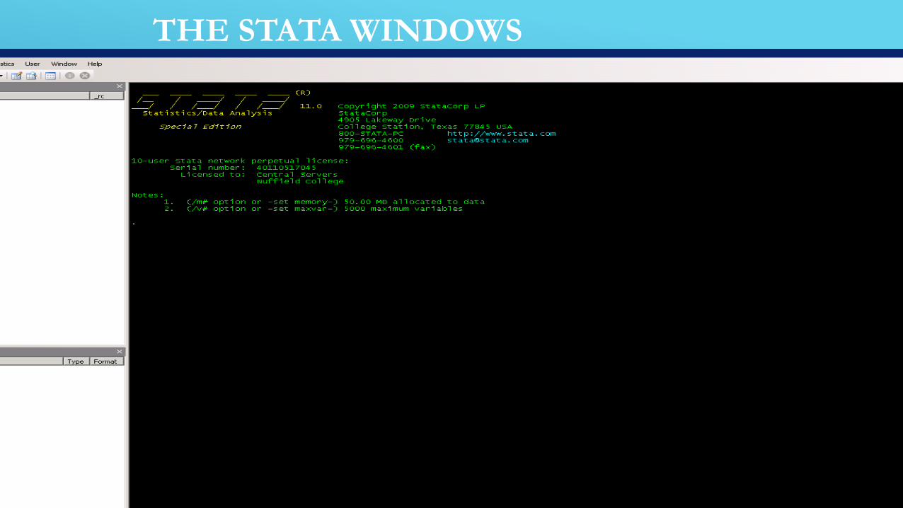
THE STATA WINDOWS

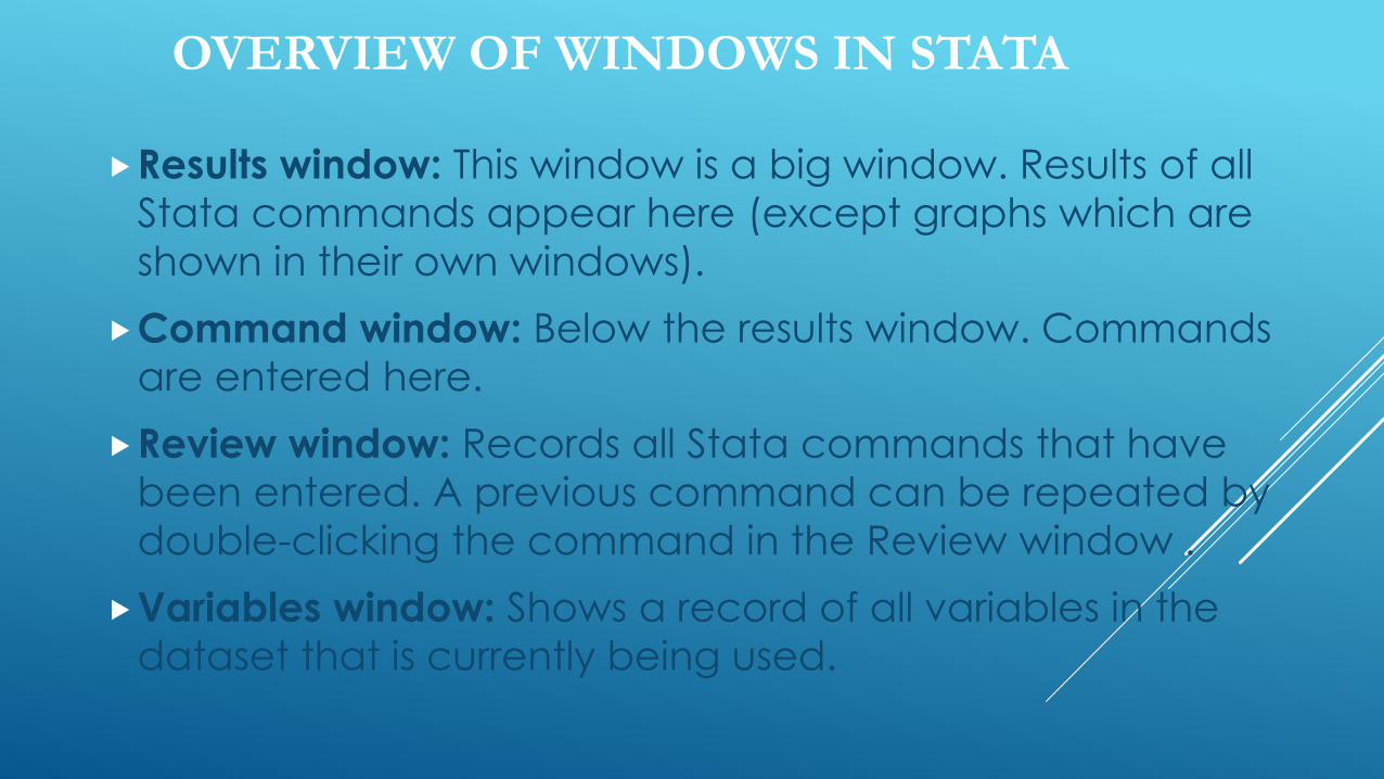
OVERVIEW OF WINDOWS IN STATA

Results window: This window is a big window. Results of all

Stata commands appear here (except graphs which are

shown in their own windows).

Command window: Below the results window. Commands

are entered here.

Review window: Records all Stata commands that have

been entered. A previous command can be repeated by

double-clicking the command in the Review window .

Variables window: Shows a record of all variables in the

dataset that is currently being used.

EXERCISE 1

GETTING TO KNOW STATA

Open Stata.

Identify the Results window, Command window, Review window, Variables window.

Set your location: cd E: or cd e: ( default directory is c: )

open the data editor and experiment with entering some data (type values and press Enter).

Exit the data editor and then clear the memory by typing clear in Command window.

WAYS OF RUNNING STATA

There are two ways to operate Stata.

Interactive mode: Commands can be typed directly into the Command window and executed by pressing Enter.

Batch mode: Commands can be written in a separate file (called a do-file) and executed together in one step.

We will use interactive mode for exercises today and batch mode in the next session.

One can also execute many commands using the menus.

SET MEMORY IN STATA

STATA’s default memory not be big enough to handle large data files. Trying to open a file that is too large return a long error message beginning with: no room to add more observations

However you can adjust the memory size to suit. So you first check the memory size of the data files by typing command – describe from the command window. With large datasets, it may be necessary to increase the memory limit. In Stata default memory is 1 megabyte ( 1024k )

SET MEMORY

For example: set memory 100m

By default, Stata assumes all files are in c:\data.

To change this working directory, type: cd foldername

Or

describe using “e:\hh_pop\pop.dta”

USING STATA DATASETS

Stata datasets always have the extension .dta.

Access existing stata dataset filename.dta by selecting File Open or by typing: use filename [, clear]

For Example: use "E:\training.dta", clear

If a dataset is already in memory (and is not required to be saved), empty memory with clear option.

To save a dataset, click or type: save filename [, replace]

Use replace option when overwriting an existing Stata (.dta) dataset.

USING STATA DATASETS

There are many ways to use or open data file in Stata software:

Manual entry by typing or pasting data into data editor

Stata format data (file contain extension ( .dta ) directly from menu

Other format data (text format extension .txt)

By using other software (like spss )we can easily convert any formatting data set ( dbf, csv, sav, xls) to stata format data (file name.dta)

insheet using E:\tafsil-5.txt,clear

(Note that: clear specifies that it is okay for the new data to replace the data that are currently in memory)

INTRODUCTION TO STATA COMMANDS (DATA MANAGEMENT)

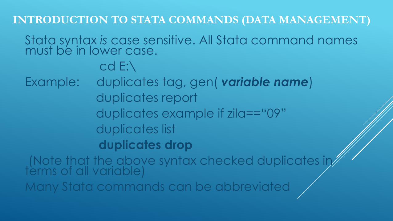
Stata syntax is case sensitive. All Stata command names must be in lower case.

cd E:\

Example: duplicates tag, gen( variable name)

duplicates report

duplicates example if zila==“09”

duplicates list

duplicates drop

(Note that the above syntax checked duplicates in terms of all variable)

Many Stata commands can be abbreviated

STATA COMMANDS

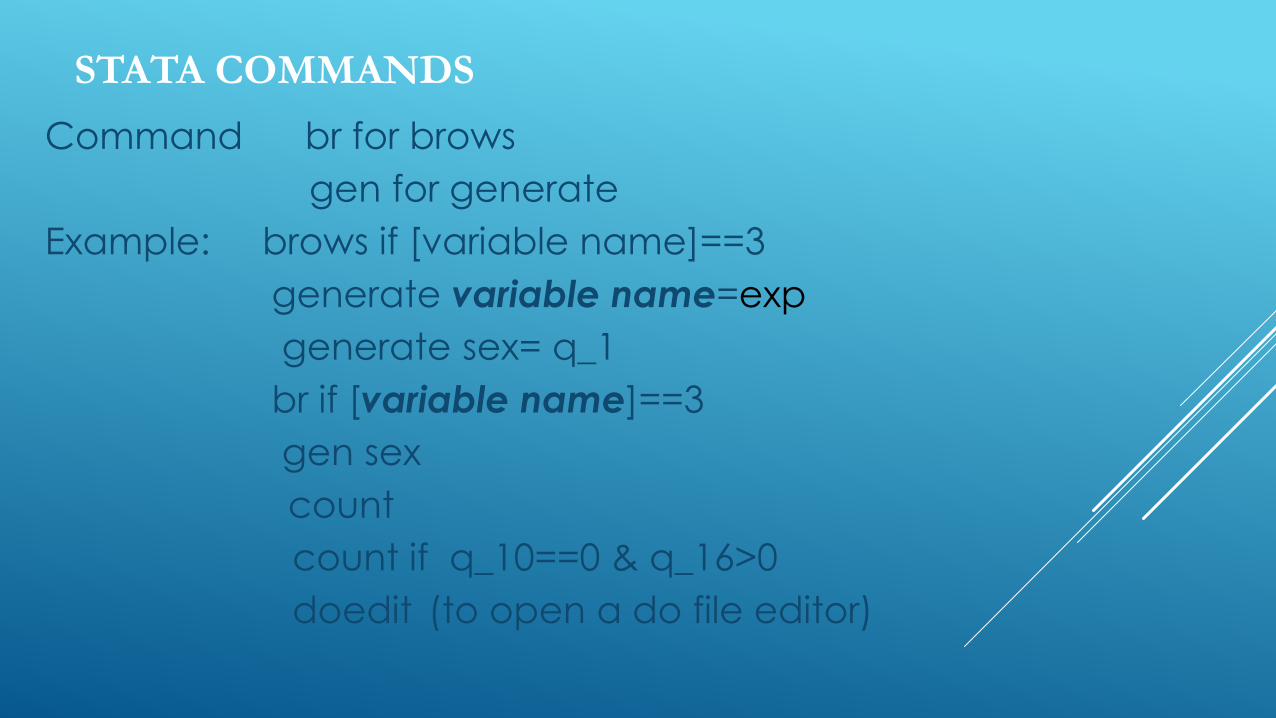
Command br for brows

gen for generate

Example: brows if [variable name]==3

generate variable name=exp

generate sex= q_1

br if [variable name]==3

gen sex

count

count if q_10==0 & q_16>0

doedit (to open a do file editor)

FORMATS VARIABLES

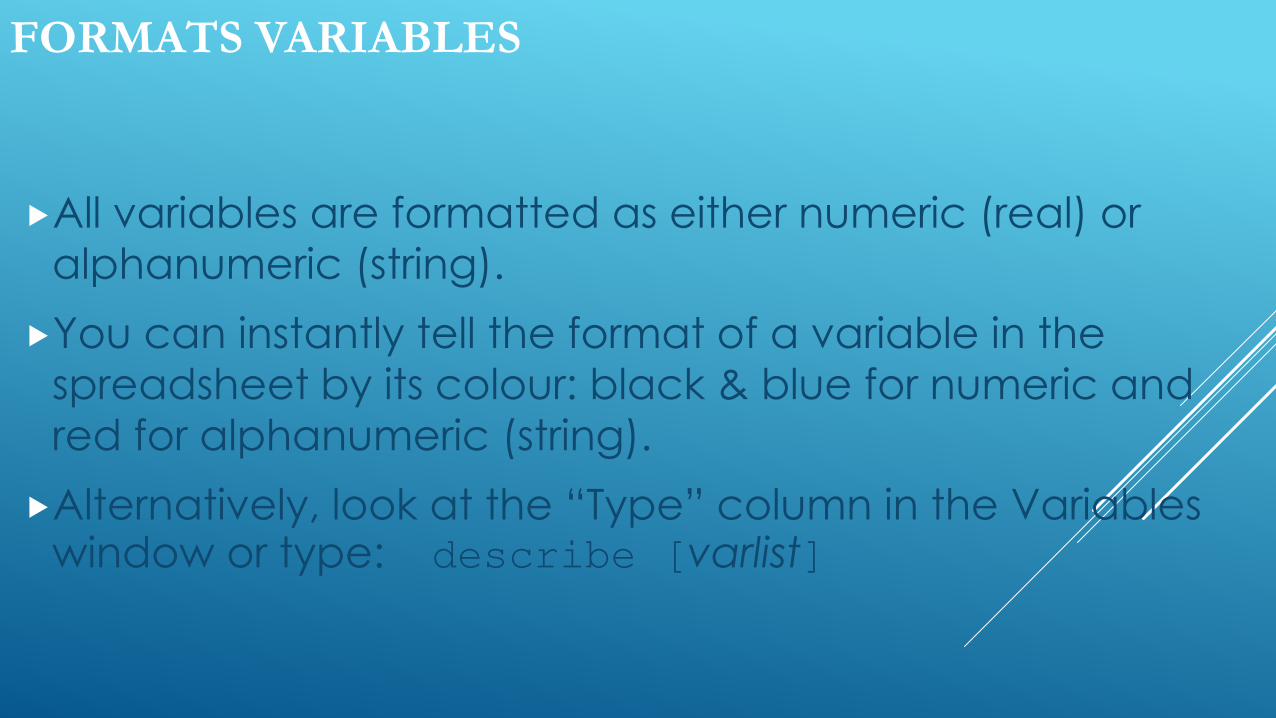
All variables are formatted as either numeric (real) or

alphanumeric (string).

You can instantly tell the format of a variable in the

spreadsheet by its colour: black & blue for numeric and

red for alphanumeric (string).

Alternatively, look at the “Type” column in the Variables window or type: describe [varlist]

FORMATS (CONT.)

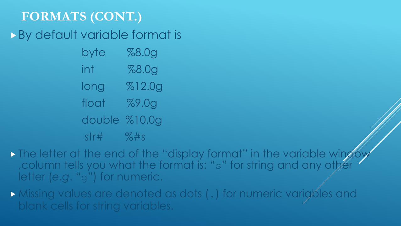
By default variable format is

byte %8.0g

int %8.0g

long %12.0g

float %9.0g

double %10.0g

str# %#s

The letter at the end of the “display format” in the variable window ,column tells you what the format is: “s” for string and any other letter (e.g. “g”) for numeric.

Missing values are denoted as dots (.) for numeric variables and blank cells for string variables.

INSPECTING THE DATA

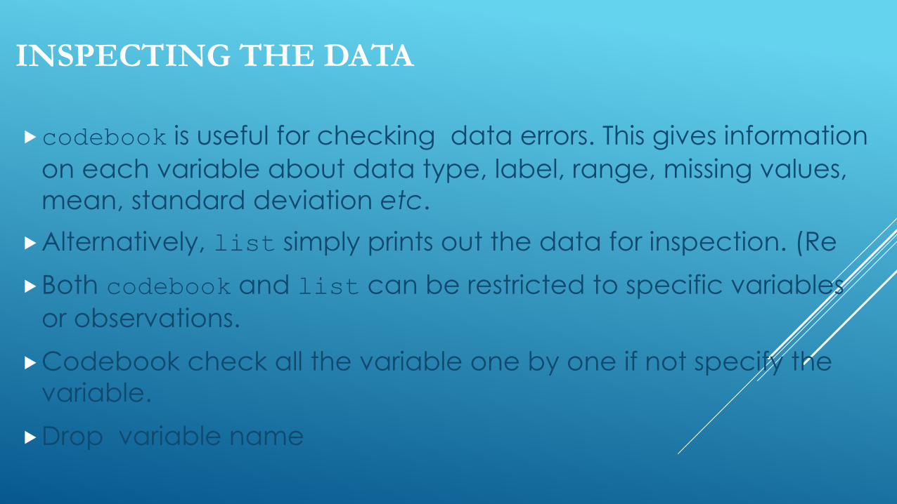
codebook is useful for checking data errors. This gives information

on each variable about data type, label, range, missing values,

mean, standard deviation etc.

Alternatively, list simply prints out the data for inspection. (Re

Both codebook and list can be restricted to specific variables

or observations.

Codebook check all the variable one by one if not specify the

variable.

Drop variable name

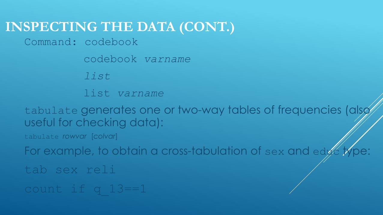
INSPECTING THE DATA (CONT.) Command: codebook

codebook varname

list

list varname

tabulate generates one or two-way tables of frequencies (also useful for checking data):

tabulate rowvar [colvar]

For example, to obtain a cross-tabulation of sex and educ type:

tab sex reli

count if q_13==1

VARIABLE IN STATA

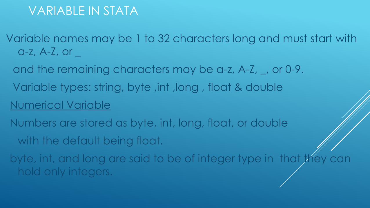
Variable names may be 1 to 32 characters long and must start with

a-z, A-Z, or _

and the remaining characters may be a-z, A-Z, _, or 0-9.

Variable types: string, byte ,int ,long , float & double

Numerical Variable

Numbers are stored as byte, int, long, float, or double

with the default being float.

byte, int, and long are said to be of integer type in that they can

hold only integers.

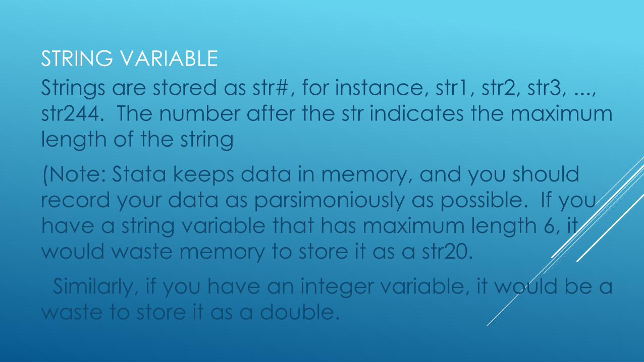
STRING VARIABLE

Strings are stored as str#, for instance, str1, str2, str3, ...,

str244. The number after the str indicates the maximum

length of the string

(Note: Stata keeps data in memory, and you should

record your data as parsimoniously as possible. If you

have a string variable that has maximum length 6, it

would waste memory to store it as a str20.

Similarly, if you have an integer variable, it would be a

waste to store it as a double.

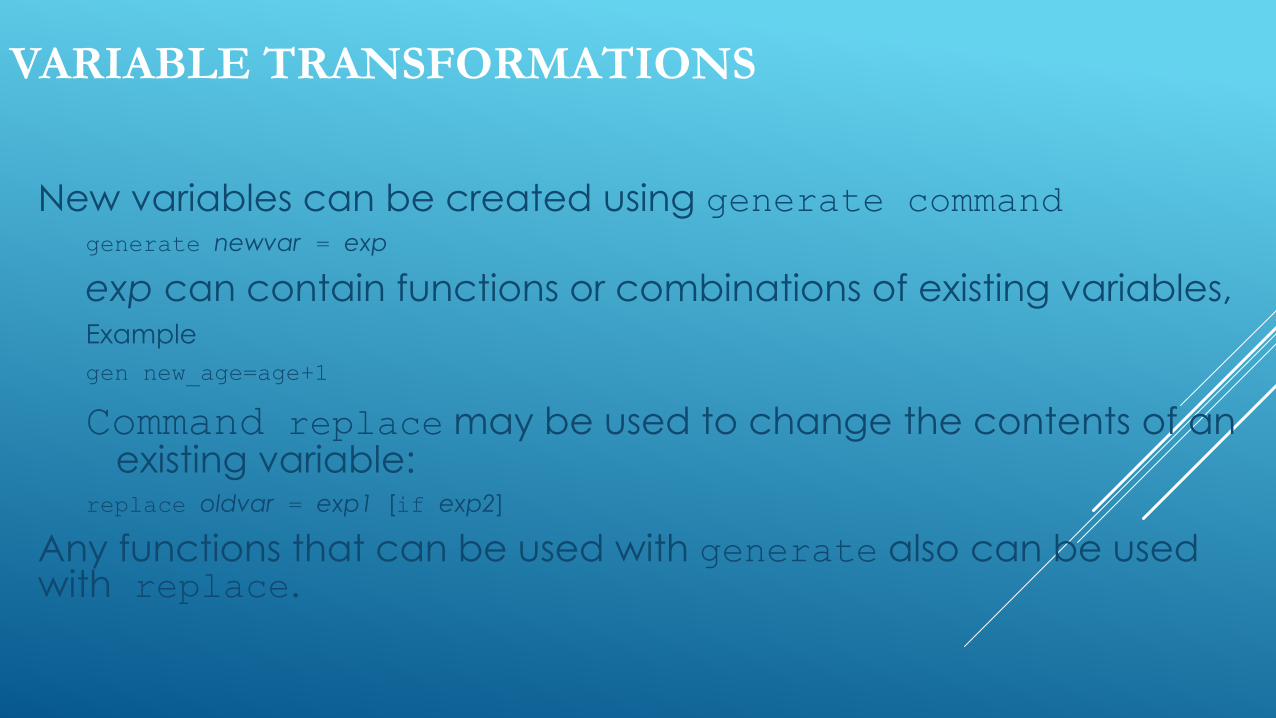
VARIABLE TRANSFORMATIONS

New variables can be created using generate command generate newvar = exp

exp can contain functions or combinations of existing variables, Example

gen new_age=age+1

Command replace may be used to change the contents of an existing variable:

replace oldvar = exp1 [if exp2]

Any functions that can be used with generate also can be used with replace.

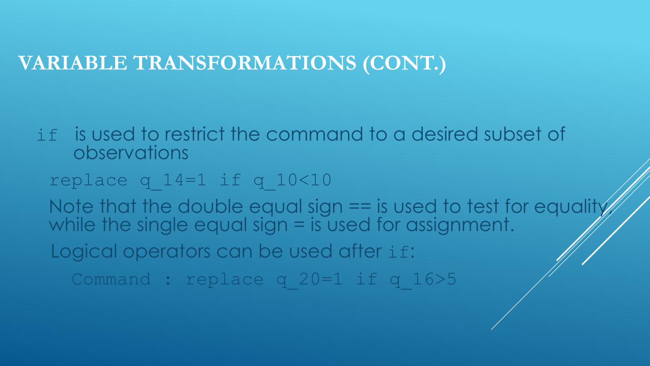
VARIABLE TRANSFORMATIONS (CONT.)

if is used to restrict the command to a desired subset of observations

replace q_14=1 if q_10<10

Note that the double equal sign == is used to test for equality, while the single equal sign = is used for assignment.

Logical operators can be used after if:

Command : replace q_20=1 if q_16>5

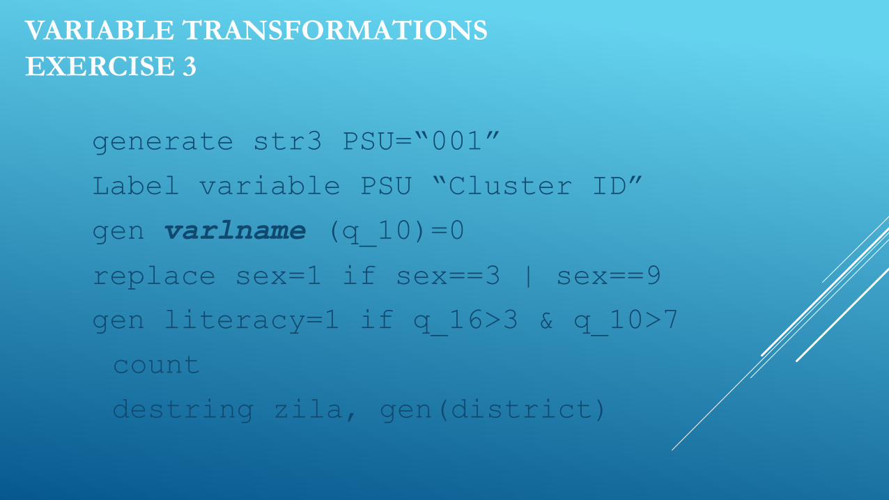
VARIABLE TRANSFORMATIONS

EXERCISE 3

generate str3 PSU=“001”

Label variable PSU “Cluster ID”

gen varlname (q_10)=0

replace sex=1 if sex==3 | sex==9

gen literacy=1 if q_16>3 & q_10>7

count

destring zila, gen(district)

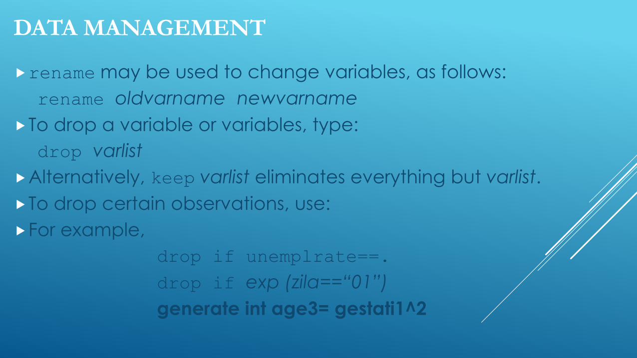
DATA MANAGEMENT

rename may be used to change variables, as follows:

rename oldvarname newvarname

To drop a variable or variables, type:

drop varlist

Alternatively, keep varlist eliminates everything but varlist.

To drop certain observations, use:

For example,

drop if unemplrate==.

drop if exp (zila==“01”)

generate int age3= gestati1^2

STATA COMMAND (EXERCISE)

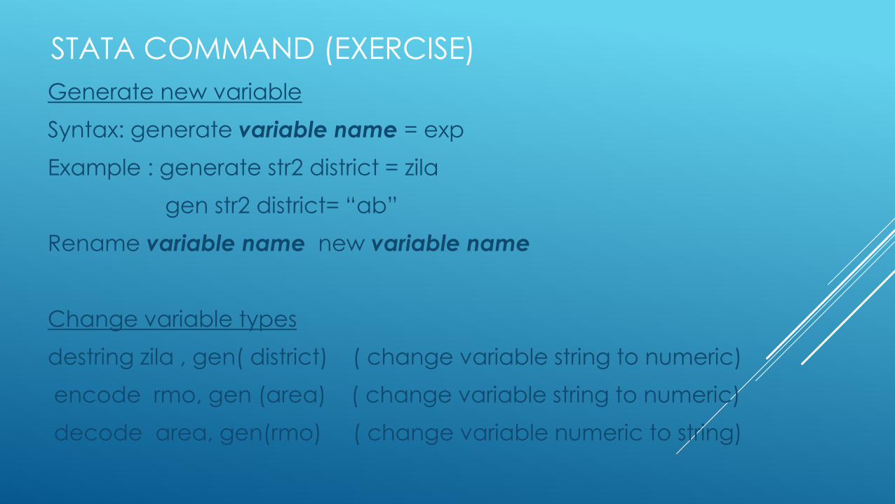
Generate new variable

Syntax: generate variable name = exp

Example : generate str2 district = zila

gen str2 district= “ab”

Rename variable name new variable name

Change variable types

destring zila , gen( district) ( change variable string to numeric)

encode rmo, gen (area) ( change variable string to numeric)

decode area, gen(rmo) ( change variable numeric to string)

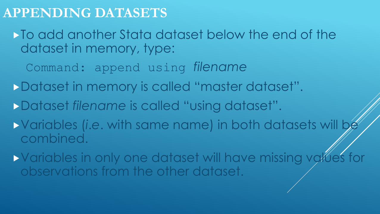
APPENDING DATASETS

To add another Stata dataset below the end of the dataset in memory, type:

Command: append using filename

Dataset in memory is called “master dataset”.

Dataset filename is called “using dataset”.

Variables (i.e. with same name) in both datasets will be combined.

Variables in only one dataset will have missing values for observations from the other dataset.

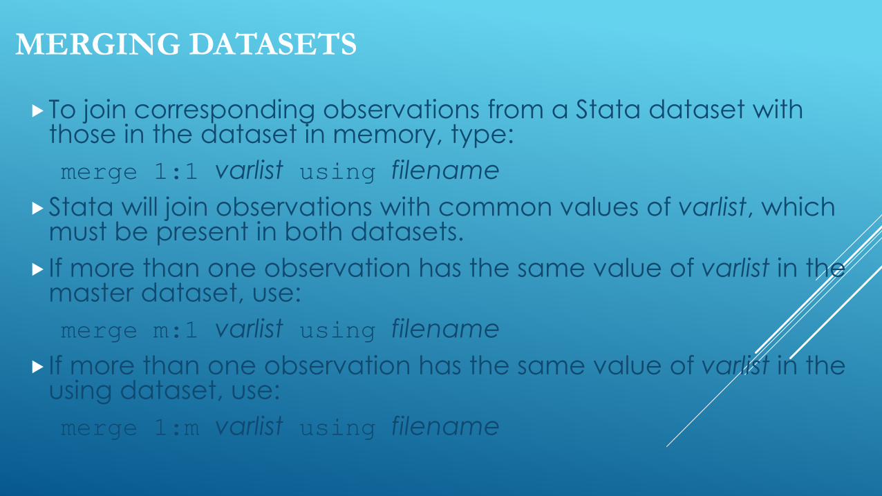
MERGING DATASETS

To join corresponding observations from a Stata dataset with those in the dataset in memory, type:

merge 1:1 varlist using filename

Stata will join observations with common values of varlist, which must be present in both datasets.

If more than one observation has the same value of varlist in the master dataset, use:

merge m:1 varlist using filename

If more than one observation has the same value of varlist in the using dataset, use:

merge 1:m varlist using filename

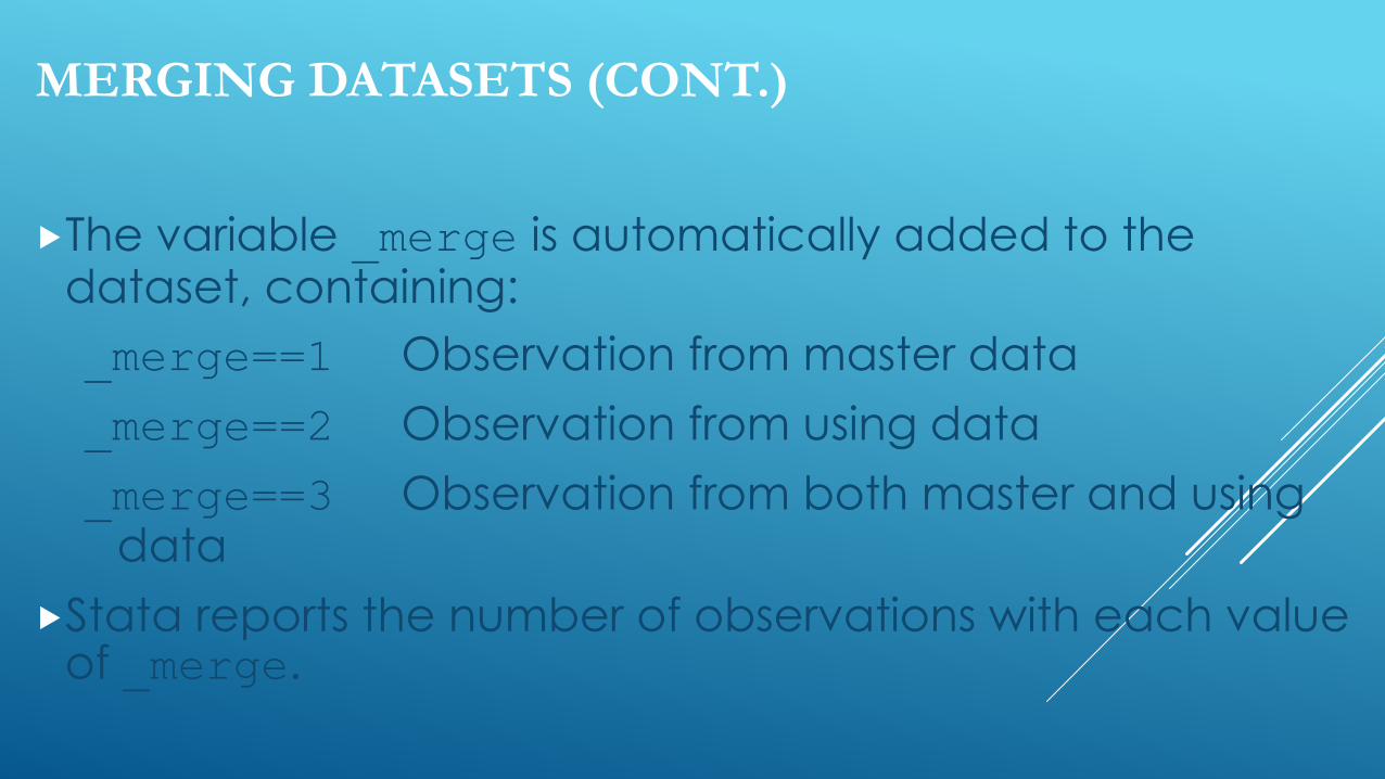
MERGING DATASETS (CONT.)

The variable _merge is automatically added to the dataset, containing:

_merge==1 Observation from master data

_merge==2 Observation from using data

_merge==3 Observation from both master and using data

Stata reports the number of observations with each value of _merge.

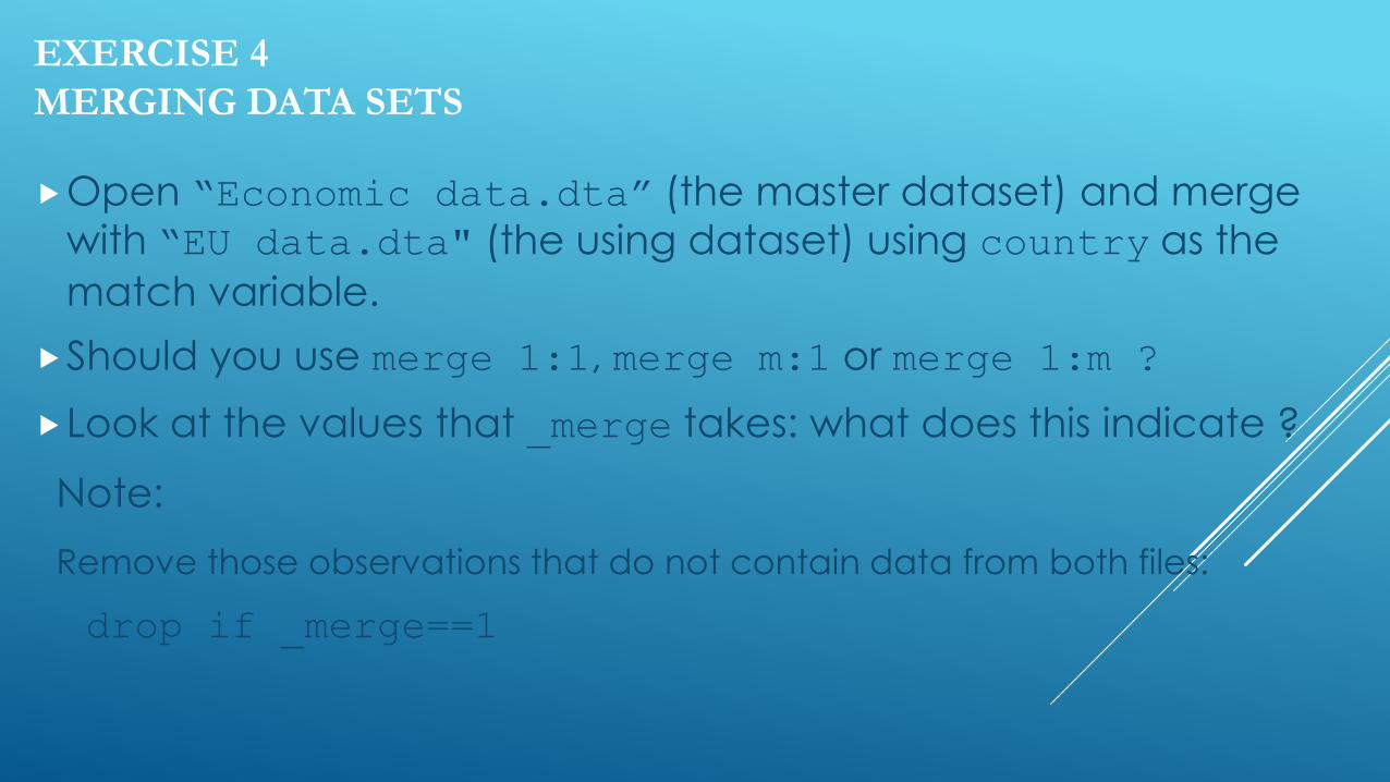
EXERCISE 4

MERGING DATA SETS

Open “Economic data.dta” (the master dataset) and merge

with “EU data.dta" (the using dataset) using country as the

match variable.

Should you use merge 1:1, merge m:1 or merge 1:m ?

Look at the values that _merge takes: what does this indicate ?

Note:

Remove those observations that do not contain data from both files:

drop if _merge==1

LOG FILES

All Stata commands and their results (except graphs)

are stored in a log file.

At the start of each Stata session, it is good practice to

open a log file, using the command:

log using filename

(where filename is chosen)

To close the log, type:

log close

DO FILE IN STATA

STATA comes with an integrated text editor called the Do-file Editor, which can be used for many task. It gets it name from the term do-file , which is a file containing a list of commands for STATA to run(called batch file). It can be used to build up a series of commands that can then be submitted to STATA all at once.

A do-file can be launched by either clicking on the Do-file editor button or by typing doedit in command window.

Instead of typing commands one-by-one in the command window, you can type all at once with in a do-file and simply run the do-file once.

DO FILE IN STATA

A do-file can be started an open the data file command and

continuous up to all the data management and analysis

commands required.

You will also have the opportunity to keep notes for each

command

. This is useful if you want to do a long data analysis or If you want

to share what you did while analyzing the data with the other

researcher.

Note: STATA will ignore a line if it is starts with an asterisk ( * ), so

you can type whatever you like on that line.

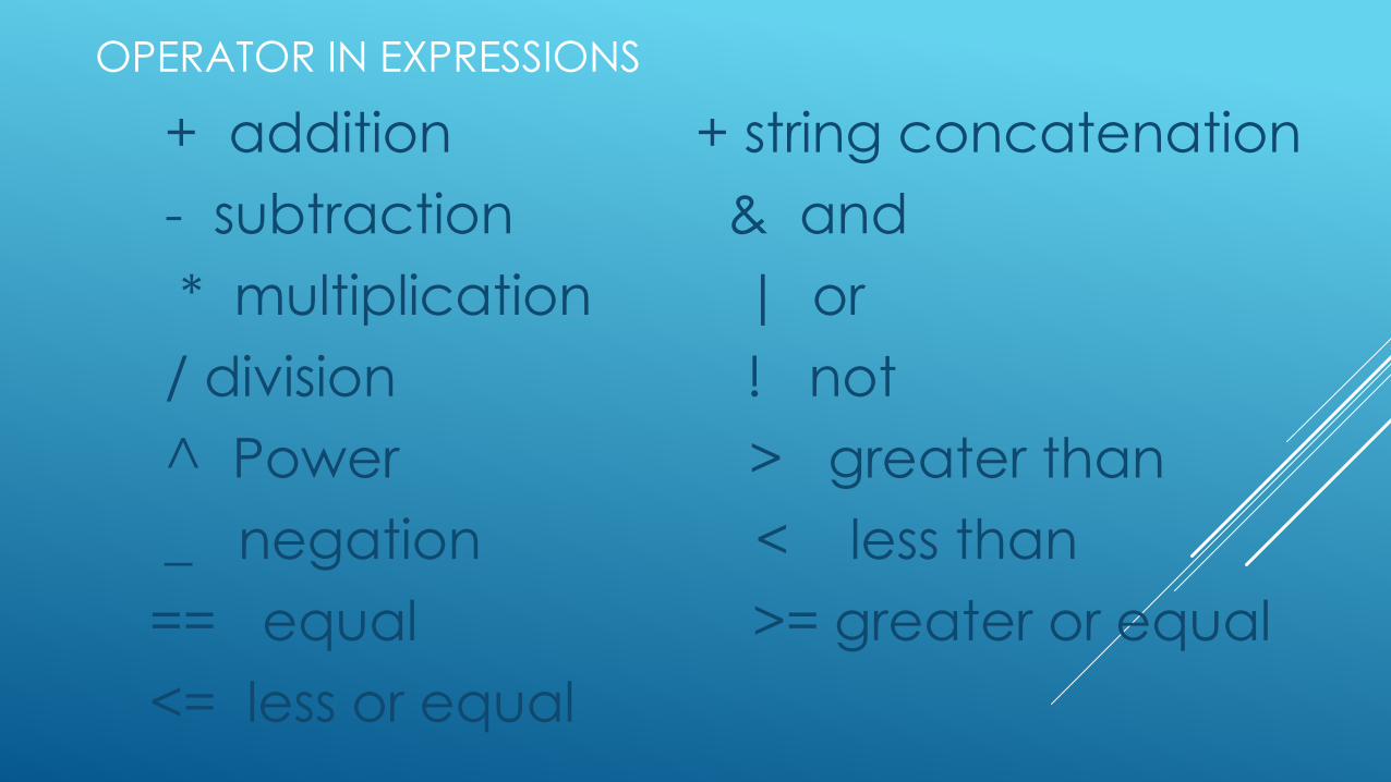
OPERATOR IN EXPRESSIONS

+ addition + string concatenation

- subtraction & and

* multiplication | or

/ division ! not

^ Power > greater than

_ negation < less than

== equal >= greater or equal

<= less or equal

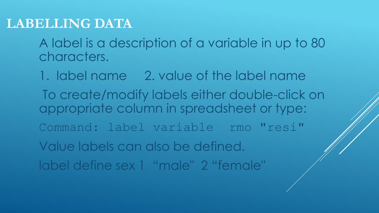
LABELLING DATA

A label is a description of a variable in up to 80 characters.

1. label name 2. value of the label name

To create/modify labels either double-click on appropriate column in spreadsheet or type:

Command: label variable rmo "resi"

Value labels can also be defined.

label define sex 1 “male" 2 “female"

COLLAPSING DATASETS

Collapse command has shown the statistics of variables

To create a dataset of means, sums etc., type:

collapse (stat) varlist1 (stat) … [[weight]],

by(varlist2)

stat can be mean, sd, sum, median or other statistics.

by(varlist2) specifies the groups over which the

means etc. are to be calculated.

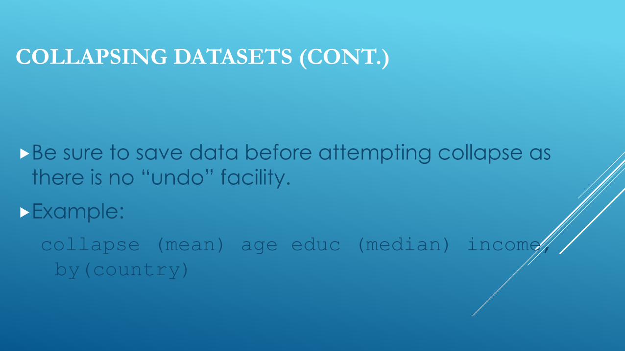
COLLAPSING DATASETS (CONT.)

Be sure to save data before attempting collapse as

there is no “undo” facility.

Example:

collapse (mean) age educ (median) income,

by(country)

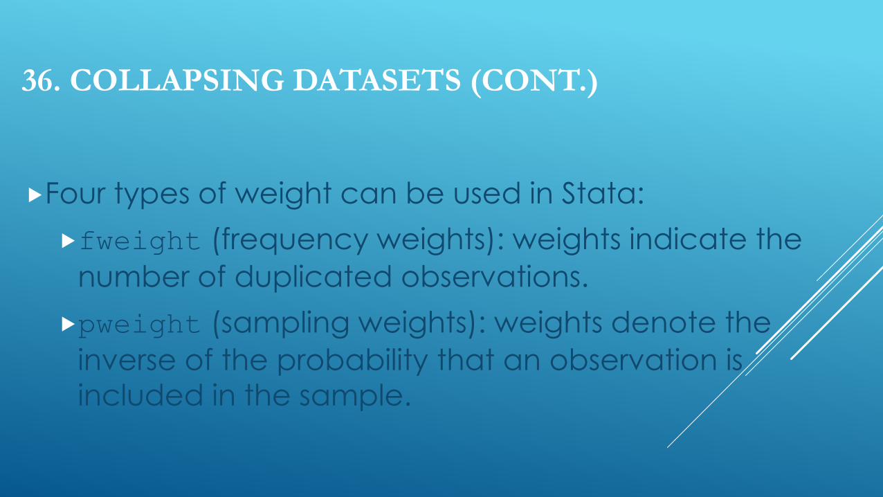
36. COLLAPSING DATASETS (CONT.)

Four types of weight can be used in Stata:

fweight (frequency weights): weights indicate the

number of duplicated observations.

pweight (sampling weights): weights denote the

inverse of the probability that an observation is

included in the sample.

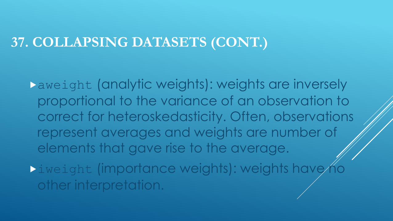
37. COLLAPSING DATASETS (CONT.)

aweight (analytic weights): weights are inversely

proportional to the variance of an observation to

correct for heteroskedasticity. Often, observations

represent averages and weights are number of

elements that gave rise to the average.

iweight (importance weights): weights have no

other interpretation.

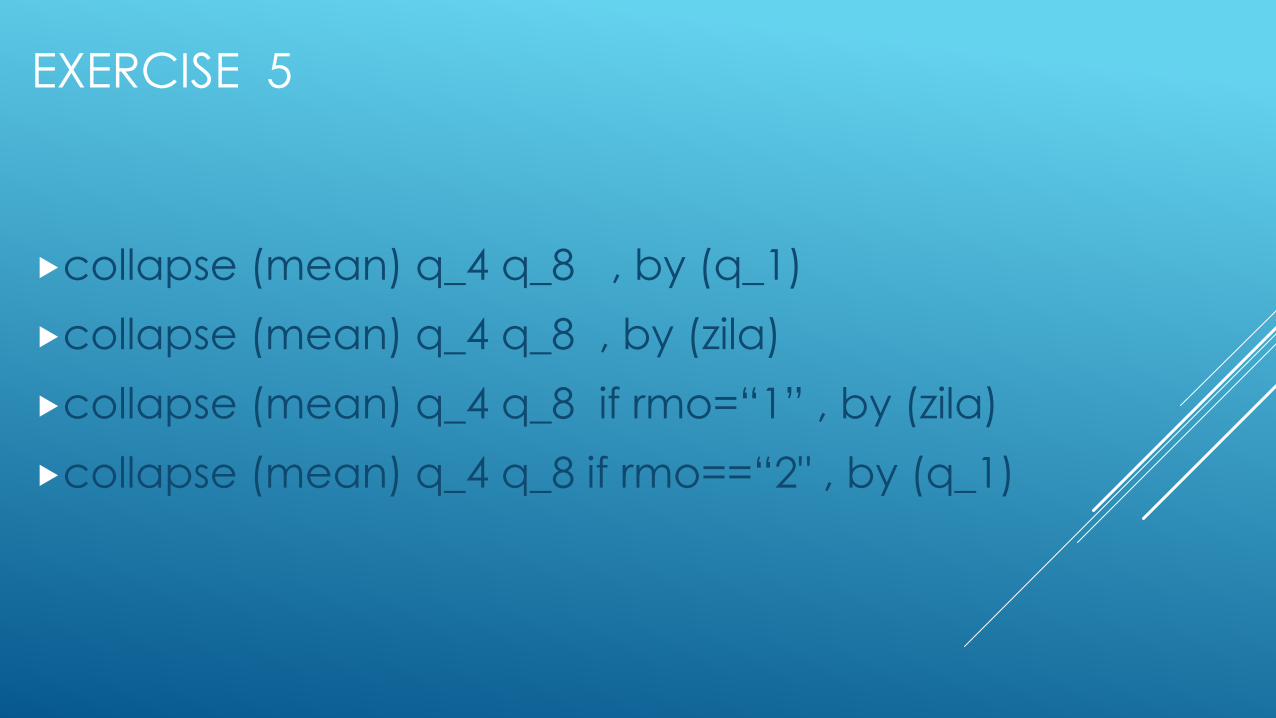
EXERCISE 5

collapse (mean) q_4 q_8 , by (q_1)

collapse (mean) q_4 q_8 , by (zila)

collapse (mean) q_4 q_8 if rmo=“1” , by (zila)

collapse (mean) q_4 q_8 if rmo==“2" , by (q_1)

OPERATIONAL DEFINITIONS OF INDICATORS

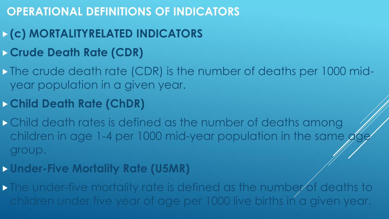
(c) MORTALITYRELATED INDICATORS

Crude Death Rate (CDR)

The crude death rate (CDR) is the number of deaths per 1000 mid-

year population in a given year.

Child Death Rate (ChDR)

Child death rates is defined as the number of deaths among

children in age 1-4 per 1000 mid-year population in the same age

group.

Under-Five Mortality Rate (U5MR)

The under-five mortality rate is defined as the number of deaths to

children under five year of age per 1000 live births in a given year.

OPERATIONAL DEFINITIONS OF INDICATORS

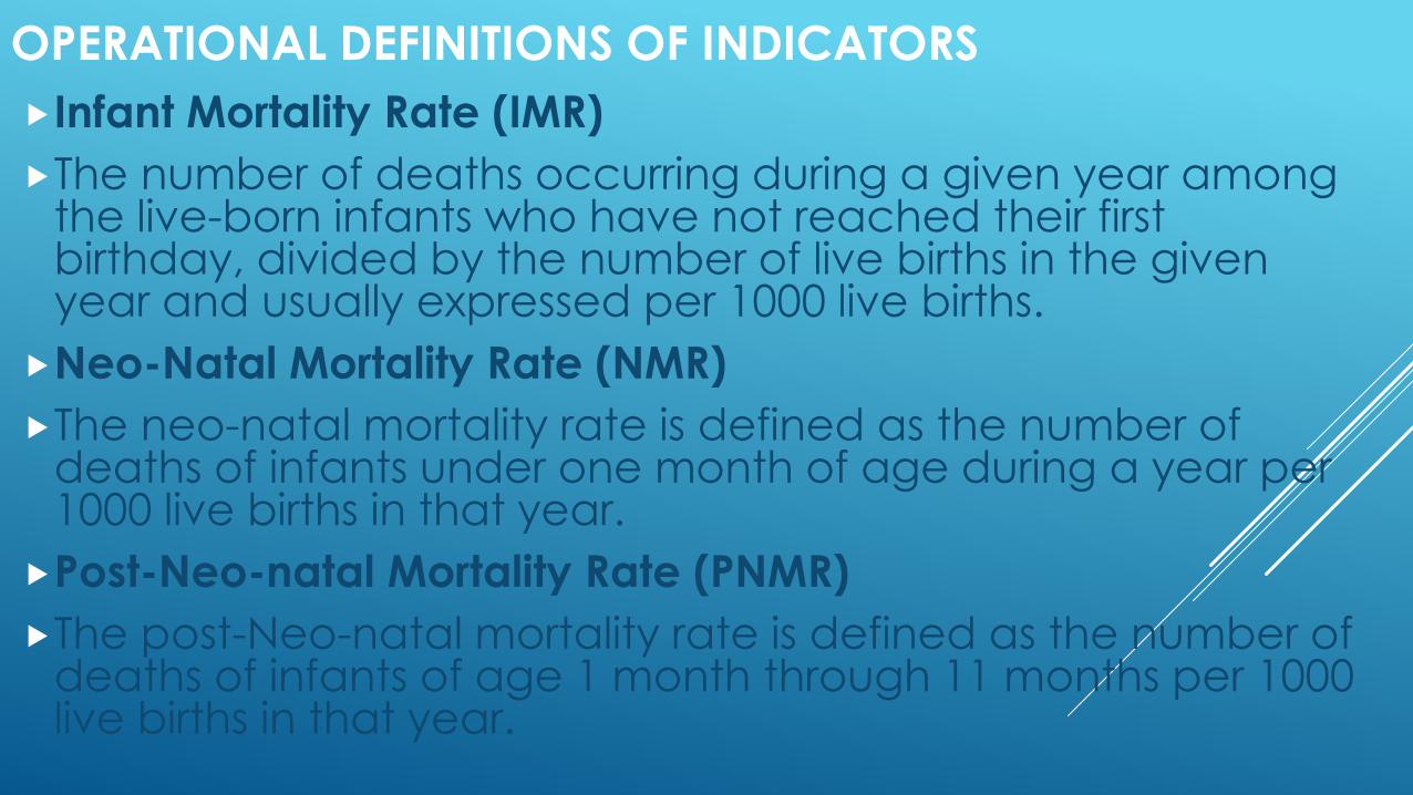
Infant Mortality Rate (IMR)

The number of deaths occurring during a given year among the live-born infants who have not reached their first birthday, divided by the number of live births in the given year and usually expressed per 1000 live births.

Neo-Natal Mortality Rate (NMR)

The neo-natal mortality rate is defined as the number of deaths of infants under one month of age during a year per 1000 live births in that year.

Post-Neo-natal Mortality Rate (PNMR)

The post-Neo-natal mortality rate is defined as the number of deaths of infants of age 1 month through 11 months per 1000 live births in that year.

OPERATIONAL DEFINITIONS OF INDICATORS

Maternal Mortality Ratio (MMR)

The maternal mortality ratio is defined as the number of

total deaths of women due to complications of

pregnancy, child birth and puerperal causes per 1000 live

births during a year.

OPERATIONAL DEFINITIONS OF INDICATORS FERTILITY RELATED INDICATORS

Crude Birth Rate (CBR)

The ratio of livebirths in a specified period (usually one calendar year) to the average population in that period (normally taken to be the mid year population). The value is conventionally expressed per 1000 population.

General Fertility Rate (GFR)

The ratio of number of live births in a specified period to the average number of women of child bearing age in the population during the period.

Age-Specific Fertility Rate (ASFR)

Number of live births occurring to women of a particular age or age group normally expressed per 1000 women in the same age- group in a given year. It is usually calculated for 5 years age groups from 15-19 to 40-44 or 15-19 to 45-49.

Total Fertility Rate (TFR)

The sum of the age-specific fertility rates (ASFRs) over the whole range of reproductive ages for a particular period (usually a year).It can be interpreted as the number of children; a woman would have during her lifetime if she were to experience the fertility rates of period at each age and no mortality till they reach to their reproductive period

OPERATIONAL DEFINITIONS OF INDICATORS

Gross Reproduction Rate (GRR)

The average number of daughters that would be born to a woman during her lifetime if

she would passed through the childbearing ages experiencing the average age-specific

fertility pattern of a given year. and no mortality till they reach to their reproductive period.

Net Reproduction Rate (NRR)

The average number of daughters that would be born to a woman if she passed through

her lifetime from birth confirm to the age specific fertility rates of a given year. This rate is similar to the gross reproduction rate and takes into account that some women will die

before completing their childbearing years. NRR means each generation of mothers is

having exactly enough daughters to replace itself in the population.

OPERATIONAL DEFINITIONS OF INDICATORS

Gross Reproduction Rate (GRR)

The average number of daughters that would be born to a woman during her lifetime if

she would passed through the childbearing ages experiencing the average age-specific

fertility pattern of a given year. and no mortality till they reach to their reproductive period.

Net Reproduction Rate (NRR)

The average number of daughters that would be born to a woman if she passed through

her lifetime from birth confirm to the age specific fertility rates of a given year. This rate is similar to the gross reproduction rate and takes into account that some women will die

before completing their childbearing years. NRR means each generation of mothers is

having exactly enough daughters to replace itself in the population.

THANK YOU ALL