NumMeth_Papers4

8/3/2019 NumMeth_Papers4

http://slidepdf.com/reader/full/nummethpapers4 1/24

Python for Derivatives Analytics in a Nutshell

Yves J. Hilpisch∗

October 16, 2010

Abstract

Financial Engineering in general and Derivatives Analytics in particular are discplineswhere theory goes hand in hand with numerical methods which in turn have to be imple-mented in some form of computer code. Python (www.python.org) lends itself very wellto this task. This brief note introduces some syntax and paradigms of Python by mainlyrelying on the example of European option pricing.

Contents

1 Python Fundamentals 2

1.1 Installing Python(x,y) . . . . . . . . . . . . . . . . . . . . . . . . . . . . . 21.2 First Steps with Python . . . . . . . . . . . . . . . . . . . . . . . . . . . . . 21.3 Array Operations . . . . . . . . . . . . . . . . . . . . . . . . . . . . . . . . . 41.4 Random Numbers . . . . . . . . . . . . . . . . . . . . . . . . . . . . . . . . 61.5 Plotting . . . . . . . . . . . . . . . . . . . . . . . . . . . . . . . . . . . . . . 6

2 European Option Pricing 8

2.1 Black-Scholes Approach . . . . . . . . . . . . . . . . . . . . . . . . . . . . . 82.2 Binomial Approach . . . . . . . . . . . . . . . . . . . . . . . . . . . . . . . . 92.3 Monte Carlo Approach . . . . . . . . . . . . . . . . . . . . . . . . . . . . . . 14

3 Selected Financial Topics 153.1 Approximation . . . . . . . . . . . . . . . . . . . . . . . . . . . . . . . . . . 153.2 Optimization . . . . . . . . . . . . . . . . . . . . . . . . . . . . . . . . . . . 183.3 Numerical Integration . . . . . . . . . . . . . . . . . . . . . . . . . . . . . . 19

4 Advanced Python Topics 19

4.1 Classes and Ob jects . . . . . . . . . . . . . . . . . . . . . . . . . . . . . . . 194.2 Data Import and Export . . . . . . . . . . . . . . . . . . . . . . . . . . . . . 21

References 24

∗Dr. Yves J. Hilpisch, Managing Director, Visixion GmbH, Rathausstrasse 75-79, 66333 Voelklingen, Ger-

many. Email [email protected], Internet www.visixion.com, www.dexision.com. Preliminary work, com-ments are welcome.

1



1 Python Fundamentals

1.1 Installing Python(x,y)

Python(x,y) is a distribution of a Python system and a number of useful libraries andtools for scientific purposes. The Web site www.pythonxy.com provides current downloadsand further information. The only drawback is that it is a Windows only version. If youuse another system, make sure to install the following:

• Python 2.6.x (www.python.org)

• NumPy 1.3.x (numpy.scipy.org)

• SciPy 0.7.x (www.scipy.org)

• Matplotlib 0.99 ( matplotlib.sourceforge.net )

• xlrd, xlwt, xutils (www.python-excel.org)

Installing either Python(x,y) or the single components is generally pretty easy and fast.You might wonder whether I do not recommend the most recent version of Python whichis already 3.x. There are two reasons. Python 2.6.x is also current and maintained by theOpen Source community. Some syntax has changed in 3.x such that the versions are notfully compatible—and most code and documentation available is for Python 2.x.

By reading this note, you will NOT learn how to code in general or learn Python fromscratch and to black belt level. However, for someone coming with C++ experience, forexample, the note illustrates fundamental aspects of Python that are useful for DerivativesAnalytics and Financial Engineering. For someone who starts out in these areas, the

topics covered provide a first glimpse at coding in general and for Derivatives Analyticsin particular. For this group, the note may act as a starting point for digging deeper intoareas of further interest.

For a thorough introduction to Python from a scientific point of view, you shouldconsult Langtangen (2009).

1.2 First Steps with Python

After starting IDLE, the standard integrated development environment which comes withany Python distribution, you should see something like this on the screen:

Python 2.6.5 (r265:79096, Mar 19 2010, 21:48:26) [MSC v.1500 32 bit (Intel)] on win32

Type "copyright", "credits" or "license()" for more information.

****************************************************************

Personal firewall software may warn about the connection IDLE

makes to its subprocess using this computer’s internal loopback

interface. This connection is not visible on any external

interface and no data is sent to or received from the Internet.

****************************************************************

IDLE 2.6.5

>>>

Before we go on and write our first module—as it is called in Python—let’s use thiscommand line interpreter for some math.

2



>>> 3+4

7

>>> 3/4

0

>>>

Addition seems to work right, but division apparently not. This is due to Pythoninterpreting ‘3’ and ‘4’ as integers such that division gives ‘0’ instead of ‘0.75’. Putting adot behind either 3 or 4 or both does the trick (i.e. we say Python that we are workingwith floats).

>>> 3.0/4

0.75

>>>

So types are important with Python. One has to be careful since Python is a dynam-ically typed language which means that there are default types which are used given aspecific context. In C++ for example you would have to assign a certain type to a variablebefore using it. Variables are defined in Python with the ‘=’ sign:

>>> a=3

>>> b=4

>>> a/b

0

>>> a=3.0

>>> a/b

0.75

>>>

Even if Python has already built in lots of functionality, most of it is stored in moduleswhich have to be imported. An example is the math module which contains, among others,trigonometric functions.

>>> sin(a)

Traceback (most recent call last):

File "<pyshell#8>", line 1, in <module>

sin(a)

NameError: name ‘sin’ is not defined

>>> from math import *>>> sin(a)

0.14112000805986721

>>>

If you want to indicate that the sin function is from the math module, you can alsoimport the module itself and not the functions that are contained therein.

>>> import math

>>> math.sin(b)

-0.7568024953079282

>>>

You can easily define functions by yourself.

3



>>> def f(x):

return x**3+x**2-2

>>> f(2)

10

>>> f(a)

34.0

>>>

Here, x**3 is for x3. Generally, if you are doing something useful which you would liketo store for later use you would not work with the command line interpreter. You wouldrather write a module, store the function in it and save it on disk. You can start this anytime by clicking on ‘New Window’ in the ‘File’ menu of IDLE. There you could store theprevious code like this:

## F i rs t P r og r am w it h P y th o n

# a _ F i r st _ P r o g ra m . p y

#

from math import *

# V a ri a bl e D e fi n it i on

a = 3 . 0

b =4

# F u nc t io n D e fi n it i on

def f(x):

return x * * 3 + x * * 2 - 2

# C a l c ul a t i o n

f_a=f(a)

f_b=f(b)

# O u tp ut

print " f ( a ) = " , f_ a

print " f ( b ) = " , f_ b

The ‘#’ sign allows to include comments in your code that is ignored by the Pythoninterpreter. Make sure when saving Python modules to always include the suffix ‘.py’.Now you can use F5 to start the program which produces the following output:

>>> ================================ RESTART ================================

>>>

f(a) = 34.0

f(b) = 78

>>>

This should be enough for the first steps with Python. We calculated, defined a functionand wrote the first module containing the function.

1.3 Array Operations

NumPy is a powerful library that allows array manipluations (linear algebra) in a compactform and at high speed. The speed comes from the implementation in C. So you have the

4



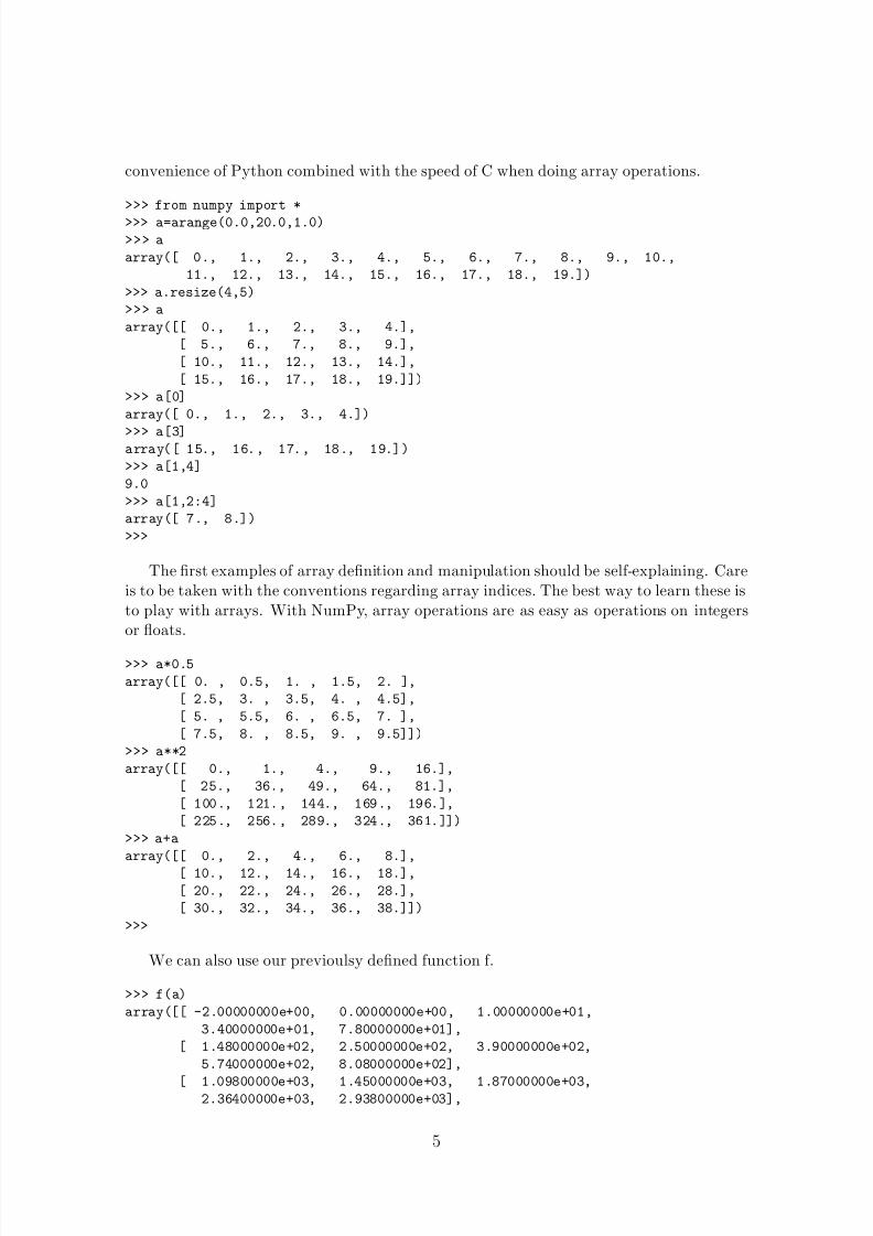
convenience of Python combined with the speed of C when doing array operations.

>>> from numpy import *

>>> a=arange(0.0,20.0,1.0)

>>> a

array([ 0., 1., 2., 3., 4., 5., 6., 7., 8., 9., 10.,

11., 12., 13., 14., 15., 16., 17., 18., 19.])

>>> a.resize(4,5)

>>> a

array([[ 0., 1., 2., 3., 4.],

[ 5., 6., 7., 8., 9.],

[ 10., 11., 12., 13., 14.],

[ 15., 16., 17., 18., 19.]])

>>> a[0]

array([ 0., 1., 2., 3., 4.])

>>> a[3]array([ 15., 16., 17., 18., 19.])

>>> a[1,4]

9.0

>>> a[1,2:4]

array([ 7., 8.])

>>>

The first examples of array definition and manipulation should be self-explaining. Careis to be taken with the conventions regarding array indices. The best way to learn these isto play with arrays. With NumPy, array operations are as easy as operations on integersor floats.

>>> a*0.5

array([[ 0. , 0.5, 1. , 1.5, 2. ],

[ 2.5, 3. , 3.5, 4. , 4.5],

[ 5. , 5.5, 6. , 6.5, 7. ],

[ 7.5, 8. , 8.5, 9. , 9.5]])

>>> a**2

array([[ 0., 1., 4., 9., 16.],

[ 25., 36., 49., 64., 81.],

[ 100., 121., 144., 169., 196.],

[ 225., 256., 289., 324., 361.]])

>>> a+a

array([[ 0., 2., 4., 6., 8.],

[ 10., 12., 14., 16., 18.],

[ 20., 22., 24., 26., 28.],

[ 30., 32., 34., 36., 38.]])

>>>

We can also use our previoulsy defined function f.

>>> f(a)

array([[ -2.00000000e+00, 0.00000000e+00, 1.00000000e+01,

3.40000000e+01, 7.80000000e+01],

[ 1.48000000e+02, 2.50000000e+02, 3.90000000e+02,

5.74000000e+02, 8.08000000e+02],

[ 1.09800000e+03, 1.45000000e+03, 1.87000000e+03,2.36400000e+03, 2.93800000e+03],

5



[ 3.59800000e+03, 4.35000000e+03, 5.20000000e+03,

6.15400000e+03, 7.21800000e+03]])

Here, the syntax e+03 is for 103. Sometimes you need to loop over arrays to checksomething. Looping is also quite intuitive in Python.

>>> b=arange(0.0,100.0,1.0)

>>> for i in range(100):

if b[i]==50.0:

print "50.0 at index no.", i

50.0 at index no. 50

>>>

The use of arange and range should be obvious. The first can produce arrays of floattype while the latter can only generate integers; and indices of arrays are always integersthat is why we loop over integers and not over floats or something else.

1.4 Random Numbers

Derivatives Analytics cannot live without random numbers, be them either pseudo-randomor quasi-random. NumPy has built in convenient functions for the generation of pseudo-random numbers in the sub-module random.

>>> from numpy.random import *

>>> b=standard_normal((4,5))>>> b

array([[-0.59317286, 0.27533818, -0.46122351, -0.05138033, -1.8371135 ],

[-1.15520074, 1.04980946, 0.31082909, 0.32662006, -0.36752163],

[ 0.66452767, -0.88077193, 1.18253972, 0.16836824, -1.40541028],

[ 0.01481426, -0.88137549, 0.74594197, -0.97360666, -0.77270426]])

>>> a+b

array([[ -0.59317286, 1.27533818, 1.53877649, 2.94861967, 2.1628865 ],

[ 3.84479926, 7.04980946, 7.31082909, 8.32662006, 8.63247837],

[ 10.66452767, 10.11922807, 13.18253972, 13.16836824, 12.59458972],

[ 15.01481426, 15.11862451, 17.74594197, 17.02639334, 18.22729574]])

>>>

1.5 Plotting

More often than not, one wants to visualze results from calculations or simulations. Themodule matplotlib is quite powerful when it comes to 2D visualizations of any kind. Themost important types of graphics for Derivatives Analytics are lines, dots and bars.

>>> from matplotlib.pyplot import *

>>> plot(a+b)

[<matplotlib.lines.Line2D object at 0x020A7E30>, <matplotlib.lines.Line2D object at

0x0218E690>, <matplotlib.lines.Line2D object at 0x0218E730>, <matplotlib.lines.Line2D

object at 0x0218E7B0>, <matplotlib.lines.Line2D object at 0x0218E830>]

>>> xlabel(’x-axis’)<matplotlib.text.Text object at 0x020BC590>

6



>>> ylabel(’y-axis’)

<matplotlib.text.Text object at 0x020BCEF0>

>>> grid(True)

>>> show()

Figure 1 shows the output. Notice that matplotlib produces five lines with fourdifferent values each which is due to the array size of 4 × 5. The next example combinesa dot sub-plot with a bar sub-plot the result of which is shown in figure 2. Here, due toresizing of the array we have only a one-dimensional set of numbers.

>>> c=resize(b,20)

>>> subplot(211)

<matplotlib.axes.AxesSubplot object at 0x0CD547F0>

>>> plot(c,’ro’)

[<matplotlib.lines.Line2D object at 0x01A44C90>]

>>> subplot(212)

<matplotlib.axes.AxesSubplot object at 0x0CF93150>

>>> bar(range(20),c)

[<matplotlib.patches.Rectangle object at 0x0D016230>, ...]

>>> show()

This is already quite all we need to implement different European option pricing algo-rithms in the next section. What may be missing will be added on the fly.

0 . 0 0 . 5 1 . 0 1 . 5

2 . 0 2 . 5 3 . 0

x - a x i s

5

0

5

1 0

1 5

2 0

y

-

a

x

i

s

Figure 1: Example of figure with matplotlib—here: lines

7



0 5 1 0 1 5 2 0

2 . 0

1 . 5

1 . 0

0 . 5

0 . 0

0 . 5

1 . 0

1 . 5

0 5

1 0 1 5

2 0

2 . 0

1 . 5

1 . 0

0 . 5

0 . 0

0 . 5

1 . 0

1 . 5

Figure 2: Example of figure with matplotlib—here: dots & bars

2 European Option Pricing

2.1 Black-Scholes Approach

The seminal model of Black and Scholes (1973) is still a benchmark for the pricing of European options stocks and indices. The analytical call option formula without dividendsis

C 0(K, T ) = S 0N(d1) − e−rT K N(d2)

d1 ≡ log(S 0/K ) + (r + 0.5σ2)T

σ√

T

d2 ≡ d1 − σ√

T

where N is the cumulative distribution function (cdf) of a standard normal random vari-able. The single variables have the following meaning, respectively:

• C 0 call option value today

• S 0 index level today

• K strike price of the option

• T time-to-maturity of the call option

• r risk-less short rate

• σ volatility of index level (standard deviation of its returns)

All we need additionally to implement the formula is the cdf for a standard normalvariable. We get this from the scipy module which contains a sub-module called stats.

#

# V al ua ti on o f E ur op ea n C al l O pt io n in B S7 3 M od el# b _ B S1 9 7 3 . p y

8



#

from scipy import stats

from math import *

# O p ti on P a ra m et e rs

s 0 = 1 05 . 00 # I n it i al I n de x L e ve l

K = 1 00 . 00 # S t ri k e L ev el

T = 1. # C al l O p ti o n M a tu r it y

r = 0 . 0 5 # C o ns t an t S ho r t R at e

v ol a = 0 . 25 # C o ns t an t V o la t il i ty o f D i ff u si o n

# A n al y ti c al F o rm u la

def BS73_Call_Value (s0,K,T,r,vola):

d 1 = ( l o g ( s 0 / K ) +( r + 0 . 5 * v o l a * * 2 )* T ) / ( v o l a * s q rt ( T ) )

d 2 = d 1 - v ol a * s qr t ( T )

B S _C = ( s 0 * s t a ts . n o r m . c d f ( d1 , 0 . 0 , 1 . 0 )-K*exp(-r*T)*stats.norm.cdf(d2,0.0,1.0))

return BS_C

# O u tp ut

print " V a lu e o f E u ro p ea n c al l o p ti o n i s ",

BS73_Call_Value(s0,K,T,r,vola)

The function BS73 Call Value gives us a benchmark value for the European call optionwith the parameters as defined in the Python module:

>>> ================================ RESTART ================================

>>>

Value of European call option is 15.6547197268

>>>

2.2 Binomial Approach

To better understand how to implement the binomial option pricing model of Cox, Rossand Rubinstein (1979), a little more background seems helpful.

There are two securities traded in the model: a risky stock index and a risk-less zero-coupon bond. The time horizon [0, T ] is divided in equidistant time intervals ∆t so thatone gets T /∆t + 1 points in time t ∈ {0, ∆t, 2 · ∆t,...,T }. The zero-coupon bond growsp.a. in value with the risk-less short rate r, Bt = B0ert where B0 > 0.

Starting from a strictly positive, fixed stock index level of S 0 at t = 0, the stock indexevolves according to the law

S t+∆t ≡ S t · m

where m is selected randomly from {u, d}. Here, 0 < d < er∆t < u ≡ eσ√ ∆t as well as

u ≡ 1d

as a simplification which leads to a recombining tree.Assuming risk-neutral valuation holds, the following relationship can be derived

S t = er∆tEQt [S t+∆t]

= er∆t(quS t + (1

−q)dS t)

Against this background, the risk-neutral (or martingale) probability is

9



q =

er∆t

−d

u − d

The value of a European call option C 0 is then obtained by discounting the final payoffsC T (S T , K ) ≡ max[S T − K, 0] at t = T to t = 0:

C 0 = e−rT EQ0 [C T ]

The discounting can be done step-by-step and node-by-node backwards starting at t =T − ∆t.

From an algorithmical point of view, one has to first generate the index level values,determines then the final payoffs of the call option and finally discounts them back. Thisis what we now will do, starting with a somewhat ‘naive’ implementation. But before

we do it, we generate a Python module which contains all parameters that we will needfor different implementations afterwards. All parameters can be imported by using theimport command and the respective filename without the suffix ‘.py’ (i.e. the filename isc Parameters.py and the module name is c Parameters).

#

# M o de l P a ra m et e rs f or E u ro p ea n C al l O pt i on a nd B i no m ia l M od e ls

# c _ P a ra m e t e rs . p y

#

from math import exp,sqrt

# O p ti on P a ra m et e rs

s 0 = 1 05 . 00 # I n it i al I n de x L e ve lK = 1 00 . 00 # S t ri k e L ev el

T = 1. # C al l O p ti o n M a tu r it y

r = 0 . 0 5 # C o ns t an t S ho r t R at e

v ol a = 0 . 25 # C o ns t an t V o la t il i ty o f D i ff u si o n

# T im e P a ra m et e rs

t = 3 # T im e I n te r va l s

d el ta = T / t # L en gt h o f T im e I nt er va l

d f = e xp ( - r * d el t a ) # D i sc o un t F a ct o r

# B i no m ia l P a ra m et e rs

u = e xp ( v o la * s q rt ( d e lt a ) ) # U p - M o v e m en t

d = 1/ u # D ow n - M o v em e n t

q = ( e xp ( r * d el t a ) -d ) /( u - d ) # M a r t in g a l e P r o b a bi l i t y

Here is now the first version of the binomial model which uses Excel-like cell iterationsextensively. We will see that there are ways to a more compact and faster implementation.

#

# V a lu a ti o n o f E u ro p ea n C al l O p ti o n i n C R R1 9 79 M od e l

# N a iv e V e rs i on ( = E xc el - l ik e I t er a ti o ns )

# d _ C R R 19 7 9 _ N a iv e . p y

#

from numpy import *

from c_Parameters import *

10



# A r ra y I n it i al i za t io n f or I nd e x L e ve ls

s = z e ro s ( ( t+ 1 , t+ 1 ) ,'float')

s [0 , 0] = s0

z = 0

for j in range (1,t+1,1):

z = z + 1

for i in range (z+1):

s [ i , j ] = s [ 0 , 0 ] * ( u ** j ) * ( d * * ( i * 2 ))

# A r ra y I n it i al i za t io n f or I nn e r V a lu es

i v = z er o s (( t + 1 ,t + 1 ),'float ')

z = 0



i v [i , j ] = round ( max ( s [ i , j ] - K , 0 ) , 8 )

z = z + 1

# V a l u at i o n

p v = z er o s (( t + 1 ,t + 1 ),'float ') # P r es e nt V al u e A rr a y

p v [: , t ] = i v [: , t ] # L as t T im e S te p I n it i al V a lu e s

z = t+ 1

for j in range (t-1,-1,-1):

z = z - 1

for i in range (z):

p v [ i , j ] = ( q * p v [ i , j + 1 ] +( 1 - q ) * p v [ i + 1 , j + 1 ] )* d f

# O u tp ut

print " V a lu e o f E u ro p ea n c al l o p ti o n i s ", p v [0 , 0 ]

The command zeros((i,j),’float’) initializes a NumPy array with dimension i × jwhere each number is of type float. A run of the module gives the following output andarrays where one can follow the three steps easily (index levels, inner values, discounting):

>>>


>>> s

array([[ 105. , 121.30377267, 140.13909775, 161.89905958],

[ 0. , 90.88752771, 105. , 121.30377267],

[ 0. , 0. , 78.67183517, 90.88752771],

[ 0. , 0. , 0. , 68.09798666]])

>>> ivarray([[ 5. , 21.30377267, 40.13909775, 61.89905958],

[ 0. , 0. , 5. , 21.30377267],

[ 0. , 0. , 0. , 0. ],

[ 0. , 0. , 0. , 0. ]])

>>> pv

array([[ 16.29293245, 26.59599847, 41.79195237, 61.89905958],

[ 0. , 5.61452766, 10.93666406, 21.30377267],

[ 0. , 0. , 0. , 0. ],

[ 0. , 0. , 0. , 0. ]])

>>>

Our alternative version makes more use of the capabilities of NumPy—the consequenceis more compact code even if it is not so easy to read in a first instance.

11



#

# V a lu a ti o n o f E u ro p ea n C al l O p ti o n i n C R R1 9 79 M od e l

# A d va n ce d V e rs i on ( = N u mP y I t er a ti o ns )

# d _ C R R 19 7 9 _ N a iv e . p y

#

from numpy import *


# A r ra y I n it i al i za t io n f or I nd e x L e ve ls

m u = a r an g e ( t+ 1 )

m u = r e s iz e ( m u , ( t + 1 , t + 1 ))

m d = t r an s po s e ( mu )

m u = u * *( m u - md )

m d = d * * md

s = s 0* mu * md

# V a l u at i o n

p v = m a xi m um ( s - K , 0)

Q u = z er o s (( t + 1 ,t + 1 ),'float ')

Q u [: , :] = q

Qd = 1 - Qu

z = 0

for i in range (t-1,-1,-1):

p v [ 0 : t -z , i ] = ( Q u [ 0 : t - z , i ]* p v [ 0 : t - z , i + 1 ]+

Qd[0:t-z,i]*pv[1:t-z+1,i+1])*df

z = z + 1

# O u tp ut

print " V a lu e o f E u ro p ea n c al l o p ti o n i s ", p v [0 , 0 ]

The valuation result is, as expected, the same for the parameter definitions from before.However, three time intervals are of course not enough to come close to the Black-Scholesbenchmark of 15.6547197268. With 1,000 time intervals, however, the algorithms comequite close to it:

>>> ================================ RESTART ================================

>>>


>>>

The major difference between the two algorithms is execution time. The second im-plementation which avoids Python iterations as much as possible is about 30 times fasterthan the first one. You should make this a principle for your own coding efforts: wheneverpossible avoid necessary iterations in Python and delegate them to NumPy. Apart fromtime savings, you generally also get more compact and readable code. A direct comparisonillustrates this point:

# N a iv e V e rs i on - - - I t e r at i on s i n P y th o n

#

# A r ra y I n it i al i za t io n f or I nn e r V a lu es

i v = z er o s (( t + 1 ,t + 1 ),'

float'

)z = 0

12





i v [i , j ] = max ( s [ i , j ] - K , 0 )

z = z + 1

# A d va n ce d V e rs i on - - - I t e r at i on s w it h N u mP y / C

#

p v = m a xi m um ( s - K , 0)

To conclude this section, I want to apply the Fast Fourier Transform (FFT) algorithmto the binomial model. Nowadays this numerical routine plays a central role in DerivativesAnalytics. It is used regularly for plain vanilla option pricing in productive environmentsin investment banks or hedge funds. In general, however, it is not applied to a binomialmodel but the application in this case is straightforward and therefore a quick win for us.1

## V a lu a ti o n o f E u ro p ea n C al l O p ti o n i n C R R1 9 79 M od e l

# F FT V er si on ( no P yt ho n i te ra ti on s at a ll )

# f _ C R R 19 7 9 _ F FT . p y

#

from numpy import *

from numpy.fft import fft,ifft


# A r ra y G e ne r at i on f or I nd e x L e ve l s

m d = a r an g e ( t+ 1 )

m u = r e s iz e ( m d [ - 1 ] , t + 1 )

m u = u * *( m u - md ) m d = d * * md

s = s 0* mu * md

# V al ua ti on b y F FT

C _T = m a xi m um ( s - K ,0 )

Q = z er os ( t +1 ,'float ')

Q [ 0 ] = q

Q [ 1 ] = 1 - q

l = s qr t (t + 1)

v 1 = i ff t ( C _T ) * l

v 2 = ( s q r t ( t + 1 )* f f t ( Q ) / ( l * ( 1 + r * d el t a ) ) ) ** t

C _0 = f ft ( v 1 * v2 ) / l

# O u tp ut

print " V a lu e o f E u ro p ea n c al l o p ti o n i s ", r e al ( C _ 0 [ 0 ] )

In this module, Python iterations are all avoided—this is possible since for Europeanoptions only the final payoffs are relevant. The speed advantage of this algorithm is againconsiderable: it is 30 times faster than our advanced algorithm from before and 900 timesfaster than the naive version.

1 Refer to Cerny (2004) for details of this method and its application to a binomial model.

13



2.3 Monte Carlo Approach

Finally, we apply Monte Carlo simulation (MCS) to value the same European call option.Here it is where pseudo-random numbers come into play. Similarly to the FFT algorithmwe only care about the final index level at T and simulate it with pseudo-random numbers.We get the following simple simulation algorithm2:

• consider the date of maturity T and write

S T = S 0 · e(r−1

2σ2)·T +σ

√ TwT (1)

• start iterating i = 1, 2,...,I

– draw a standard normally distributed pseudo-random number wT (i)

– determine at T the index level S T (i) by applying the pseudo-random number to

equation (1)

– determine the inner value of the call at T as max[S T (i) − K, 0]

• iterate until i = I

• sum up all inner values at T , take the average and discount back to t = 0:

C 0(K, T ) ≈ e−rT 1

I

I

max[S T (i) − K, 0]

—this is the MCS estimator for the European call option value

Although the word ‘iterating’ sounds like looping over arrays we can again avoid array loops

completely on the Python level. The Python/NumPy implementation is really compact—only 5 lines of code for the core algorithm. With another 5 lines we can produce a histogramof the index levels at T as displayed in figure 3.

#

# V a lu a ti o n o f E u ro p ea n C al l O p ti o n v ia M o nt e C a rl o S i mu l at i on

# g _ MC S . py

#

from numpy.random import *

from matplotlib.pyplot import *


from numpy import *

# V al ua ti on v ia M CS

p at h s = 3 00 0 00

r a nd = s t a n d ar d _ n o rm a l ( p a t h s )

s T = s 0 * e x p ( (r - 0 . 5 * v o l a * * 2 )* T + s q r t ( T ) * v o la * r a n d )

pv = sum (maximum(sT-K,0)*exp(-r*T))/paths

print " V a lu e o f E u ro p ea n c al l o p ti o n i s ", pv

# G r ap h ic a l A n al y si s

figure()

hist(sT,100)

xlabel('s to ck v al ue a t T ')

ylabel('

frequency'

)show()

14



5 0 0 5 0 1 0 0 1 5 0 2 0 0 2 5 0

i n d e x l e v e l a t T

0

5 0 0 0

1 0 0 0 0

1 5 0 0 0

2 0 0 0 0

f

r

e

q

u

e

n

c

y

Figure 3: Histogram of simulated stock index levels at T

The algorithm produces a quite accurate estimate for the European call option valuealthough the implementation is rather simplistic (i.e. there are, for example, no variance

reduction techniques involved):

>>> ================================ RESTART ================================

>>>


>>>

3 Selected Financial Topics

3.1 Approximation

It is often the case in Derivatives Analytics that one has to approximate something to drawconclusions. Two important approximation techniques are regression and interpolation.3

The type of regression we consider is called ordinary least squares regression (OLS). Inits most simple form, ordinary polynomials x, x2, x3,... are used to approximate a desiredfunction y = f (x) given a number N of obervations (y1, x1), (y2, x2), ..., (yN , xN ). Say wewant to approximate f (x) with a polynomial of order 2, g(x) = a1 + a2 · x + a3 · x2 wherethe ai are regression parameters. The task is then to

mina1,a2,a3

N n

(yn − g(xn; a1, a2, a3))

2

Glasserman (2004) is a comprehensive reference on the Monte Carlo method.3 Brandimarte (2006, sec. 3.3) introduces into these techniques.

15



As an example, we want to approximate the cosine function over the interval [0, π/2]given 20 observations. The code is straightforward since NumPy has built-in functions

polyfit and polyval. From polyfit you get the minimizing regression parameters back,while you can use them with polyval to generate values based on these parameters. Theresult is shown in figure 4 for three different regression functions.

#

# O r di n ar y L ea s t S q ua r es R e gr e ss i on

# h _ RE G . py

#

from numpy import *


# R e g r es s i o n

x = l i ns p ac e ( 0 .0 , p i /2 , 2 0 )

y = c os ( x)

g 1 = p o ly f it ( x , y , 0)

g 2 = p o ly f it ( x , y , 1)

g 3 = p o ly f it ( x , y , 2)

g 1y = p o ly v al ( g 1 , x)

g 2y = p o ly v al ( g 2 , x)

g 3y = p o ly v al ( g 3 , x)


plot(x,y,'y')

plot(x,g1y,'rx ')

plot(x,g2y,'

bo'

)plot(x,g3y,'g >')

The concept of interpolation is much more involved but nevertheless almost as straight-forward in applications. The most common type of interpolation is with cubic splines forwhich you find functions in the sub-module scipy.interpolate. The example remainsthe same and the code is as compact as before while the result—see figure 5—seems almostperfect.

#

# C u bi c S pl i ne I n te r po l at i on

# i _ S PL I N E . p y

#from numpy import *

from scipy.interpolate import *


# I n t e r po l a t i on

x = l i ns p ac e ( 0 .0 , p i /2 , 2 0 )

y = c os ( x)

g p = s p lr e p (x , y , k= 3 )

g y = s pl e v (x , gp , d e r = 0)


plot(x,y,'b')

plot(x,gy,'ro ')

16



0 . 0 0 . 2 0 . 4 0 . 6 0 . 8 1 . 0 1 . 2 1 . 4

1 . 6

0 . 2

0 . 0

0 . 2

0 . 4

0 . 6

0 . 8

1 . 0

1 . 2

Figure 4: Approximation of cosine function (line) with constant regression (red crosses), linearregression (blue dots) and quadratic regression (green triangles)

0 . 0 0 . 2 0 . 4 0 . 6 0 . 8 1 . 0 1 . 2 1 . 4 1 . 6

0 . 0

0 . 2

0 . 4

0 . 6

0 . 8

1 . 0

1 . 2

Figure 5: Approximation of cosine function (line) with cubic splines interpolation (red dots)

17



Roughly speaking, cubic splines interpolation is (intelligent) regression between everytwo observation points with a polynomial of order 3. This is of course much more flexible

than a single regression with a polynomial of order 2. Two drawbacks in algorithmic termsare, however, that the observations have be ordered in the x-dimension. Furthermore, cubicsplines are of limited or no use for higher dimensional problems where OLS regression isapplicable as easy as in the two-dimensional world.

3.2 Optimization

Strictly speaking, regression and interpolation are two special forms of optimization (somekind of minimization). However, optimization techniques are needed much more oftenin Derivatives Analytics. An important area is, for example, the calibration of modelparameters to a given set of market-observed option prices or implied volatilities.

The two major approaches are global and local optimization. While the first looks for aglobal minimum or maximum of a function (which does not have to exist at all), the secondlooks for a local minimum or maximum. As an example, we take the sine function over theintervall [−π, 0] with a minimum function value of −1 at π/2. Again, the module scipy

delivers respective functions via the sub-module optimize. The code looks like follows:

#

# F in di ng a M in im um

# j _ OP T . py

#

from numpy import *

from scipy.optimize import *

# F in di ng a M in im um

def y(x):

if x < - p i or x > 0 :

return 0. 0

return sin(x)

g m in = b r u te ( y , ( ( - p i , 0 , 0 . 01 ) , ) , f i n i sh = None )

l mi n = f mi n ( y ,- 0 . 5)

# O u tp ut

print " G l ob a l M i ni m um i s ", g mi n

print " L oc al M in im um i s " , l mi n

Both functions brute (global brute force algorithm) and fmin (local convex optimiza-tion algorithm) also work in multi-dimensional settings. In general, the solution of thelocal optimization is strongly dependent on the initialization; here the −0.5 did quite wellin reaching π/2 as the solution.

>>> ================================ RESTART ================================

>>>

Optimization terminated successfully.

Current function value: -1.000000

Iterations: 18

Function evaluations: 36

Global Minimum is -1.57159265359

Local Minimum is [-1.57080078]>>>

18



3.3 Numerical Integration

It is not always possible to analytically integrate a given function. Then numerical inte-

gration often comes into play. We want to check numerical integration where we can do itanalytically as well:

10

exdx

The value of the integral is e1 − e0 ≈ 1.7182818284590451. For numerical integration,again scipy helps out with the sub-module integrate which contains the function quad,implementing a numerical quadrature scheme4:

#

# N u me r ic a ll y I n te g ra t e a F u nc t io n

# j _ IN T . py#

from numpy import *

from scipy.integrate import *

# N u m e ri c a l I n t e g ra t i o n

def f(x):

return exp(x)

I nt = q ua d (lambda u : f ( u ), 0 , 1 )[ 0 ]

# O u tp ut

print " V al ue o f t he I nt eg ra l i s" , I nt

The output of the numerical integration equals the analytical value (with rounding):

>>> ================================ RESTART ================================

>>>

Value of the Integral is 1.71828182846

>>>

4 Advanced Python Topics

4.1 Classes and ObjectsSo far, we came by mainly with modules and functions. The dominating coding paradigmof our time is, however, object-oriented programming. For example, the popularity of C++ for Derivatives Analytics stems to a great extent from the fact that it brings alongpowerful object-orientation.

On a rather basic level, almost anything is an object in Python. What we want to donow is to implement new classes of objects, i.e. we go one level higher. For example, wecan define a new class for European call options. A class is characterized by its attributeswhich are stored in a function with name init and so-called methods, like the valuationfunction of Black and Scholes (1973) as already implemented before. Here is a sample codefor two classes:

4 Brandimarte (2006, ch. 4) introduces into numerical integration.

19



#

# T wo O pt io n C la ss es

# k _ CL A SS . p y

#

from numpy import *

from scipy import stats

# C l as s D e fi n it i on s

class Option :

def __init__ ( self ,s0,K,T,r,vola):

self . s 0 = s 0

self . K = K

self . T = T

self . r = rself . v ol a = v ol a

def Value ( self ):

s 0 , K , T , r , v ol a = self .s0, self .K , self .T , self .r , self .vola

d 1 = ( l o g ( s 0 / K ) +( r + 0 . 5 * v o l a * * 2 )* T ) / ( v o l a * s q rt ( T ) )

d 2 = d1 - v o la * s q rt ( T )

v a l = ( s 0 * s t a ts . n o r m . c d f ( d1 , 0 . 0 , 1 . 0 )

-K*exp(-r*T)*stats.norm.cdf(d2,0.0,1.0))

return va l

class Option_Vega (Option):

def Vega ( self ):

s 0 , K , T , r , v ol a = self .s0, self .K , self .T , self .r , self .vola

d 1 = ( l o g ( s 0 / K ) +( r + ( 0 . 5 * v o la * * 2 ) ) * T ) / ( v o la * s q r t ( T ) )

return s 0 * s t a ts . n o r m . c d f ( d1 , 0 . 0 , 1 . 0 ) * s q r t ( T )

The working becomes clear after executing the module and defining option objects byparameterizing the different classes:

>>> ================================ RESTART ================================

>>>

>>> o1 = Option(105.,100.,1.0,0.05,0.25)

>>> o1.Value()

15.654719726823579

>>> o1.Vega()


File "<pyshell#18>", line 1, in <module>

o1.Vega()

AttributeError: Option instance has no attribute ’Vega’

>>> o2 = Option_Vega(105.,100.,1.0,0.05,0.25)

>>> o2.Value()

15.654719726823579

>>> o2.Vega()

73.345040765170197

>>>

The class Option only contains a method called Value. The value of the option objecto1 can be retrieved via invoking the method as in o1.Value(). However, the class Option

20



has no method to calculate the Vega5 of the option. This, however, is what is included inthe class Option Vega. This class has been defined on the basis of the Option class via

class Option Vega(Option) and inherits the attributes and methods of the other class.That is why we parameterize an object of this class in the same way and why we cancalculate its value in the same way.

4.2 Data Import and Export

Saving and loading Python modules is really simple. However, the need to save and loadPython objects also arises frequently. In this section, I want to illustrate two simpleways of storing data permanently. The first is to save and load Python objects in a purePython envrionment. The second stores date in and retrieves data from Microsoft Excelspreadsheet files. This is a very important functionality since Excel still is one of the

dominating front-office tools in investment banks, hedge funds, etc.Suppose we want to save our two option objects o1 and o2 to a file on disk. A respective

session in IDLE could look like the following:

>>> ================================ RESTART ================================

>>>

>>> o1 = Option(105.,100.,1.0,0.05,0.25)

>>> o2 = Option_Vega(105.,100.,1.0,0.05,0.25)

>>> from cPickle import *

>>> options = open("Option_Container","w")

>>> dump(o1,options)

>>> dump(o2,options)

>>> options.close()>>> options

<closed file ’Option_Container’, mode ’w’ at 0x02DE2AC0>

>>> ================================ RESTART ================================

>>>

>>> options = open("Option_Container","r")

>>> o1=load(options)

>>> o2=load(options)

>>> o1.Value()

15.654719726823579

>>> o1.Vega()


File "<pyshell#50>", line 1, in <module>o1.Vega()

AttributeError: Option instance has no attribute ’Vega’

>>> o2.Vega()

73.345040765170197

>>> options.close()

>>>

Notice that the objects are loaded in the sequence as stored. And you can never know(if you didn’t save the information as well) how many objects are there in the file. So itcould be a good idea to store the two option objects not separately but as a list.

5

The Vega of an option is the first derivative of the option value with respect to the volatility, i.e. ∂C 0/∂σ .

21



>>> options = open("Option_Container_2","w")

>>> dump((o1,o2),options)

>>> options.close()

>>> ================================ RESTART ================================

>>>

>>> from cPickle import *

>>> options = open("Option_Container_2","r")

>>> o = load(options)

>>> o

(<__main__.Option instance at 0x03875080>, <__main__.Option_Vega instance at 0x039F5F58>)

>>> len(o)

2

>>> o[1]

<__main__.Option_Vega instance at 0x039F5F58>

>>> o[0]

<__main__.Option instance at 0x03875080>>>> o[0].Value()

15.654719726823579

>>> o[1].Vega()

73.345040765170197

>>>

This seems to make live much easier. The next and last topic is to read and writedata from and to Excel spreadsheets. To this end, a sample Excel workbook is needed. Iproduced one with DAX index quotes from calender week 34 (source: finance.yahoo.com).The file’s name is DAX.xls and it contains data as displayed in figure 6

Figure 6: Excel sample sheet with DAX quotes from calender week 34; source: fi-nance.yahoo.com

To access and print the data contained in the Excel file, a module like this does the job:

#

# R e ad i ng D at a f ro m E xc e l W o rk b oo k s

# m _ E x ce l _ R e ad . p y

#

from xlrd import open_workbook

# O pe n W or kb oo k , R ea d a nd P r in t

x ls = o p en _ wo r kb o ok ('DAX.xls')

for s in xls.sheets():print 'Sheet:',s.name

22



print 'W o r k sh e e t h a s',s.nrows,'r ow s w it h d at a'

print 'W o r k sh e e t h a s',s.ncols,'c o lu m ns w it h d at a'

for ro w in range (s.nrows):

d at a = []

fo r col in range (s.ncols):

data.append( st r ( s . c e l l ( r o w , c o l ) . v a l u e ) )

print " ," . j o i n ( d a t a )

print

This module, once started, produces the following output:

>>> ================================ RESTART ================================

>>>

Sheet: DAX Quotes

Worksheet has 6 rows with data

Worksheet has 7 colums with dataDate,Open,High,Low,Close,Volume,Adj Close

Aug 27, 2010,5,899.99,5,957.32,5,845.49,5,951.17,26,027,900,5,951.17

Aug 26, 2010,5,937.27,5,948.91,5,896.52,5,912.58,23,078,700,5,912.58

Aug 25, 2010,5,925.48,5,954.96,5,837.90,5,899.50,29,686,600,5,899.50

Aug 24, 2010,5,962.87,5,975.83,5,869.30,5,935.44,26,305,300,5,935.44

Aug 23, 2010,6,017.19,6,055.23,5,995.37,6,010.91,19,657,100,6,010.91

>>>

A friend of mine is a seasoned investor and has some exposure to the DAX index. Toplease him, I will now manipulate the Close and Adj Close values such that they reflect

a strong gain to 6,500.00 on Friday’s closing.

#

# W r it i ng D at a i n E xc e l W o rk b oo k s

# m _ E x c el _ W r i te . p y

#

from xlutils.copy import copy

from xlrd import open_workbook

# O pe n W or kb oo k , C op y I t , C ha n ge V al ue , O v er w ri t e i t

x ls = o p en _ wo r kb o ok ('DAX.xls',formatting_info= True )

w b = c op y ( xl s ) # W r it a bl e C op y O nl y

w sh = w b . g et _ sh e et ( 0 ) # G et F ir st S he et

wsh.write(1,4, '6 , 5 0 0 . 0 0') # M a ni p ul a te D at awsh.write(1,6, '6 , 5 0 0 . 0 0') # D it o

wb.save('DAX.xls') # S av e U n de r S am e F i le n am e ( O v e rw r it e )

The workaround with a copy of the original workbook is necessary here. You could alsosave the changed copy under a different filename to preserve the old Excel file.

23



References

[1] Black, Fischer and Myron Scholes (1973): “The Pricing of Options and Corpo-rate Liabilities.” Journal of Political Economy , Vol. 81, No. 3, 638-659.

[2] Brandimarte, Paolo (2006): Numerical Methods in Finance and Economics. 2nded., John Wiley & Sons, Hoboken, New Jersey.

[3] Cerny, Ales (2004): “Introduction to Fast Fourier Transform in Finance.” Journal

of Derivatives, Vol. 12, No. 1, 73-88.

[4] Cox, John, Stephen Ross und Mark Rubinstein (1979): “Option Pricing: ASimplified Approach.” Journal of Financial Economics, Vol. 7, No. 3, 229-263.

[5] Glasserman, Paul (2004): Monte Carlo Methods in Financial Engineering. SpringerVerlag, New York et.al.

[6] Langtangen, Hans Petter (2009): A Primer on Scientific Programming with

Python. Springer Verlag, Berlin.

24

NumMeth_Papers4

Documents

Transcript of NumMeth_Papers4