NumericalMethodsforOrdinary … reason for rewriting the equations as a system of two coupled...

Numerical Methods for Ordinary

Differential Equations

By Brian D. Storey

1. Introduction

Differential equations can describe nearly all systems undergoing change. They areubiquitous is science and engineering as well as economics, social science, biology,business, health care, etc. Many mathematicians have studied the nature of theseequations and many complicated systems can be described quite precisely withcompact mathematical expressions. However, many systems involving differentialequations are so complex, or the systems that they describe are so large, that apurely mathematical representation is not possible. It is in these complex systemswhere computer simulations and numerical approximations are useful.

The techniques for solving differential equations based on numerical approxima-tions were developed before programmable computers existed. It was common tosee equations solved in rooms of people working on mechanical calculators. As com-puters have increased in speed and decreased in cost, increasingly complex systemsof differential equations can be solved on a common PC. Currently, your laptopcould compute the long term trajectories of about 1 million interacting moleculeswith relative ease, a problem that was inaccessible to the fastest supercomputersjust 5 or 10 years ago.

This chapter will describe some basic methods and techniques for the solutionof differential equations using your laptop and MATLAB, your soon to be favoriteprogram. We will review some basics of differential equations, though this will not bemathematically formal: this you will learn in your math and physics courses. Nextwe will review some basic methods for numerical approximations and introduce theEuler method (the simplest method). We will provide a lot of detail of how to write’good’ algorithms using the Euler method as an example. Next we will discuss errorapproximation and discuss fancier techniques. We will then discuss stability and’stiff’ equations. Finally we will unleash the full power of MATLAB and look intotheir built in solvers.

2. Describing physics with differential equations

Just to review, a simple differential equation usually has a form

dy

dt= f(y, t) (2.1)

where dy/dt means the change in y with respect to time and f(y, t) is any functionof y and time. Note that the derivative of the variable, y, depends upon itself. Thereare many different notations for d/dt, common ones include y and y′.

TEX Paper

2 Numerical Methods for ODEs

X

Mass, m

Spring, K

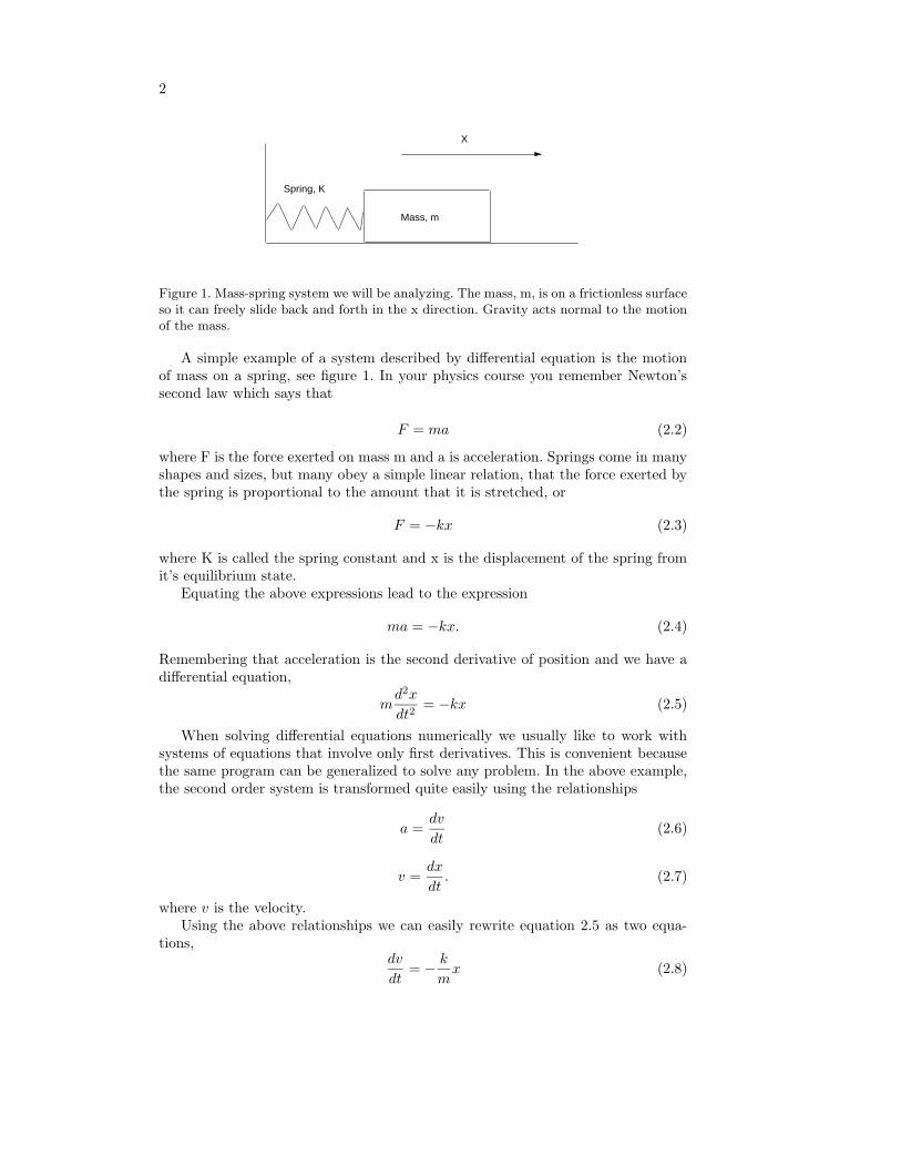
Figure 1. Mass-spring system we will be analyzing. The mass, m, is on a frictionless surfaceso it can freely slide back and forth in the x direction. Gravity acts normal to the motionof the mass.

A simple example of a system described by differential equation is the motionof mass on a spring, see figure 1. In your physics course you remember Newton’ssecond law which says that

F = ma (2.2)

where F is the force exerted on mass m and a is acceleration. Springs come in manyshapes and sizes, but many obey a simple linear relation, that the force exerted bythe spring is proportional to the amount that it is stretched, or

F = −kx (2.3)

where K is called the spring constant and x is the displacement of the spring fromit’s equilibrium state.

Equating the above expressions lead to the expression

ma = −kx. (2.4)

Remembering that acceleration is the second derivative of position and we have adifferential equation,

md2x

dt2= −kx (2.5)

When solving differential equations numerically we usually like to work withsystems of equations that involve only first derivatives. This is convenient becausethe same program can be generalized to solve any problem. In the above example,the second order system is transformed quite easily using the relationships

a =dv

dt(2.6)

v =dx

dt. (2.7)

where v is the velocity.Using the above relationships we can easily rewrite equation 2.5 as two equa-

tions,dv

dt= −

k

mx (2.8)

Numerical Methods for ODEs 3

dx

dt= v. (2.9)

The reason for rewriting the equations as a system of two coupled equations willbecome clear as we proceed. We say that the equations are coupled because thederivatives of velocity are related to the position and the derivative of position isrelated to the velocity.

Exercise: DEQ 1 Show that equations 2.5 is satisfied by x(t) =x0cos(

√

k/mt) for the initial condition x(t = 0) = x0 and v(t = 0) = 0.This states that the spring is pulled back to the position x0 and releasedfrom rest. Plot the solution with MATLAB.

3. Dimensionless equations

Before implementing a method to solve differential equations, let us take a side tripinto dimensionless equations. While this section may seem weird at first, over timeyou will start to realize the value of rescaling your equations so that they have nophysical dimensions.

When constructing solutions to differential equations it is always convenient torecast the equations into a form that has no dimensions, i.e. the equations do notdepend upon parameters that have units such as meters, seconds, etc. The reason isthat rescaling the equations will always reduce the number of free parameters thatcan be varied. Referring back to equations 2.9 & 2.8 we might think that we havefour free parameters: k, m, and x0. When we remove the dimensions we find thatthere are no free parameters, i.e. all systems behave the same. Physically, lookingparameters with no dimensions makes sense; nature cannot depend upon the unitsthat people have created.

To create non-dimensional equations we are simply scaling variables by con-stants. Let us use the * superscript to denote variables with no dimensions. Theequations have three variables, position, velocity, and time. To create a non-dimensionalvariable we simply perform the transformation

x(t)∗ =x(t)

x0(3.1)

where the time dependent position is scaled by the initial condition. We coulduse any length scale that we like (the size of your foot would work just fine),however the initial position is a convenient scale because then the initial conditionin dimensionless variables is always x∗ = 1. Now let us rewrite the equations usingthe following non-dimensional variables

v(t)∗ =v(t)

v(3.2)

t∗ =t

t(3.3)

where v and t are the velocity and time scale, constants that we will leave generalfor now. Applying these transformations to equation 2.9 yields

x0t

dx(t)∗

dt∗= vv(t)∗. (3.4)


Since we left the velocity and time scale arbitrary we can set them to be anythingthat we would like. It is easy to see that Equation 3.4 would be convenient if

v =x0t. (3.5)

This scaling would make equation 2.9 become

dx(t)∗

dt∗= v(t)∗. (3.6)

in dimensionless form, the same as it was in dimensional form.Applying the non-dimensional scaling to equation 2.8 yields,

v

t

dv(t)∗

dt∗= −

kx0m

x(t)∗. (3.7)

recalling that v = x0/t and collecting all the constants on the right-hand-side ofthe equation yields.

dv(t)∗

dt∗= −

kt2

mx(t)∗. (3.8)

Since the time scale, t, was arbitrary we see that it would be convenient if t =√

k/m. This scaling results in a system of equations with no free parameters!

dv(t)∗

dt= −x(t)∗ (3.9)

dx(t)∗

dt= v(t)∗. (3.10)

with initial conditionsx(t = 0)∗ = 1 (3.11)

v(t = 0)∗ = 0 (3.12)

What this non-dimensional scaling means is that we can solve the system ofequations once. We can plot the solution in non-dimensional form and anyone canfind dimensional solutions by multiplying the solution by a constant. Instead ofsolving the equations for each choice of parameters, we only have to solve it once.

4. Taylor Series

When solving equations such as 2.8 & 2.9 we often have information about theinitial state of the system and would like to understand how the system will evolvewith time. We need a way to integrate this equation forward in time, given thestarting state. At the heart of such approximations is the Taylor series.

Consider an arbitrary function and assume that we have all the informationabout the function at the origin (x=0) and we would like to construct an approxi-mation for x > 0. As an example let’s construct an approximation for the functionex, given only information at the origin. Let’s assume that we can create a polyno-mial approximation to the original function, f , i.e.

f = a+ bx+ cx2 + dx3 + ... (4.1)


0 0.5 1 1.5 21

2

3

4

5

6

7

8

exp(x)

1+x+x2/2+x3/6

1+x+x2/2

1+x

X

f(X

)

Figure 2. Taylor series approximation of the function ex. We have included the first threeterms in the expansion, it is clear that the approximation is valid for larger and larger xas more terms are retained.

where we will solve for the unknown coefficients a, b, c, d, etc.The simplest approximation might be to take the derivative and extrapolate the

function forward, precisely we mean,

f = f(x = 0) +df

dx

∣

∣

∣

∣

x=0

x, (4.2)

where the notation df/dx|x=0 means you take the derivative of the function withrespect to x and then evaluate that derivative at the point x = 0. Since e0 = 1 ,this approximation for our test case reduces to

f = 1 + x. (4.3)

This approximation to the original function is plotted in figure 2. We see thatthe approximation works well when x is small and deviates further away, this isexpected. By using the extrapolation technique we have simply stated that thevalue of the function and its derivative must be the same in both the real functionand the approximation.

We can improve the approximation by matching the second derivative at theorigin as well, i.e.

f(x = 0) = a = f(x = 0) (4.4)

df

dx

∣

∣

∣

∣

∣

x=0

= b =df

dx

∣

∣

∣

∣

x=0

(4.5)

d2f

dx2

∣

∣

∣

∣

∣

x=0

= 2c =d2f

dx2

∣

∣

∣

∣

x=0

(4.6)

if we continued this approximation to higher and higher derivatives we would obtainthe expression


0 5 10 15 20 2510

−16

10−14

10−12

10−10

10−8

10−6

10−4

10−2

100

Number of terms

Err

or

Figure 3. Error in the Taylor series approximation of the function ex as more terms areincluded in the sum. We see that the fundamental accuracy limit is hit at the roundofferror of ε = 10−16 when 15 terms are included in the Taylor series. The error is computedas the difference between the true function and the Taylor approximation at x = 1.

f(x) = f(x = 0) + xdf

dx

∣

∣

∣

∣

x=0

+x2

2

d2f

dx2

∣

∣

∣

∣

x=0

+x3

6

d3f

dx3

∣

∣

∣

∣

x=0

+ ...xn

n!

dnf

dxn

∣

∣

∣

∣

x=0

(4.7)

Applying approximation 4.7 to our example function shows that the approxi-mation improves as more terms are included. See figure 2 where we have plottedthe series up to terms of x3. The error for the approximation in the exponentialfunction with the Taylor series as more terms are included is plotted in Figure 3.

Exercise: DEQ 2 Write out the first 4 terms of the Taylor series for thefunction f(x) = sin(x). Plot the true function and the approximationas each term is added on the interval 0 < x < π. Compute and plot theerror in the approximation at each order.

Exercise: DEQ 3 Write out the first 4 terms of the Taylor series forthe function f(x) = ln(x) about the point x = 3. Plot the true functionand the approximation as each term is added on the interval 3 < x < 4.Compute and plot the error in the approximation at each order.

5. Your first numerical method: Euler’s method

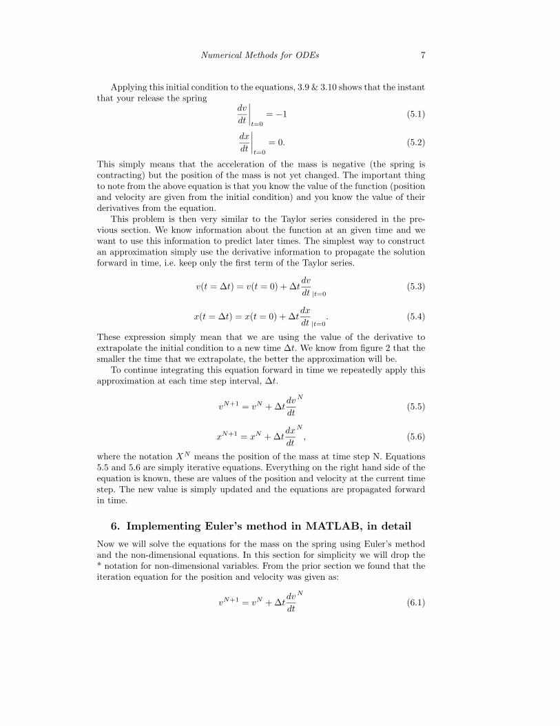
When solving an equation such as the motion of the mass on the spring it is oftendescribed as an initial value problem. This means that you often know the initialstate of the system and the equations tell you how the system will evolve with time.The initial state of the system might be that you pull back the spring, hold theblock at rest, and let go. The initial condition is then x = x0 and v = 0, the springis displaced but held still until you release.


Applying this initial condition to the equations, 3.9 & 3.10 shows that the instantthat your release the spring

dv

dt

∣

∣

∣

∣

t=0

= −1 (5.1)

dx

dt

∣

∣

∣

∣

t=0

= 0. (5.2)

This simply means that the acceleration of the mass is negative (the spring iscontracting) but the position of the mass is not yet changed. The important thingto note from the above equation is that you know the value of the function (positionand velocity are given from the initial condition) and you know the value of theirderivatives from the equation.

This problem is then very similar to the Taylor series considered in the pre-vious section. We know information about the function at an given time and wewant to use this information to predict later times. The simplest way to constructan approximation simply use the derivative information to propagate the solutionforward in time, i.e. keep only the first term of the Taylor series.

v(t = ∆t) = v(t = 0) + ∆tdv

dt |t=0(5.3)

x(t = ∆t) = x(t = 0) + ∆tdx

dt |t=0. (5.4)

These expression simply mean that we are using the value of the derivative toextrapolate the initial condition to a new time ∆t. We know from figure 2 that thesmaller the time that we extrapolate, the better the approximation will be.

To continue integrating this equation forward in time we repeatedly apply thisapproximation at each time step interval, ∆t.

vN+1 = vN +∆tdv

dt

N

(5.5)

xN+1 = xN +∆tdx

dt

N

, (5.6)

where the notation XN means the position of the mass at time step N. Equations5.5 and 5.6 are simply iterative equations. Everything on the right hand side of theequation is known, these are values of the position and velocity at the current timestep. The new value is simply updated and the equations are propagated forwardin time.

6. Implementing Euler’s method in MATLAB, in detail

Now we will solve the equations for the mass on the spring using Euler’s methodand the non-dimensional equations. In this section for simplicity we will drop the* notation for non-dimensional variables. From the prior section we found that theiteration equation for the position and velocity was given as:

vN+1 = vN +∆tdv

dt

N

(6.1)


0 5 10 15 20 25 30 35−1.5

−1

−0.5

0

0.5

1

1.5

time

X(t

)

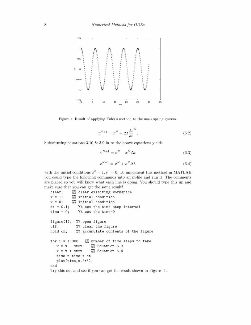
Figure 4. Result of applying Euler’s method to the mass spring system.

xN+1 = xN +∆tdx

dt

N

, (6.2)

Substituting equations 3.10 & 3.9 in to the above equations yields

vN+1 = vN − xN∆t (6.3)

xN+1 = xN + vN∆t. (6.4)

with the initial conditions x0 = 1, v0 = 0. To implement this method in MATLAByou could type the following commands into an m-file and run it. The commentsare placed so you will know what each line is doing. You should type this up andmake sure that you can get the same result!

clear; %% clear exisiting workspace

x = 1; %% initial condition

v = 0; %% initial condition

dt = 0.1; %% set the time step interval

time = 0; %% set the time=0

figure(1); %% open figure

clf; %% clear the figure

hold on; %% accumulate contents of the figure

for i = 1:300 %% number of time steps to take

v = v - dt*x %% Equation 6.3

x = x + dt*v %% Equation 6.4

time = time + dt

plot(time,x,’*’);

end

Try this out and see if you can get the result shown in Figure 4.


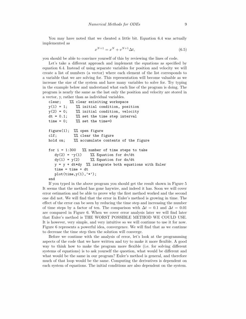
You may have noted that we cheated a little bit. Equation 6.4 was actuallyimplemented as

xN+1 = xN + vN+1∆t, (6.5)

you should be able to convince yourself of this by reviewing the lines of code.Let’s take a different approach and implement the equations as specified by

equation 6.4. Instead of using separate variables for position and velocity we willcreate a list of numbers (a vector) where each element of the list corresponds toa variable that we are solving for. This representation will become valuable as weincrease the size of the system and have many variables to solve for. Try typingin the example below and understand what each line of the program is doing. Theprogram is nearly the same as the last only the position and velocity are stored ina vector, y, rather than as individual variables.

clear; %% clear exisiting workspace

y(1) = 1; %% initial condition, position

y(2) = 0; %% initial condition, velocity

dt = 0.1; %% set the time step interval

time = 0; %% set the time=0

figure(1); %% open figure

clf; %% clear the figure

hold on; %% accumulate contents of the figure

for i = 1:300 %% number of time steps to take

dy(2) = -y(1) %% Equation for dv/dt

dy(1) = y(2) %% Equation for dx/dt

y = y + dt*dy %% integrate both equations with Euler

time = time + dt

plot(time,y(1),’*’);

end

If you typed in the above program you should get the result shown in Figure 5It seems that the method has gone haywire, and indeed it has. Soon we will covererror estimation and be able to prove why the first method worked and the secondone did not. We will find that the error in Euler’s method is growing in time. Theeffect of the error can be seen by reducing the time step and increasing the numberof time steps by a factor of ten. The comparison with ∆t = 0.1 and ∆t = 0.01are compared in Figure 6. When we cover error analysis later we will find laterthat Euler’s method is THE WORST POSSIBLE METHOD WE COULD USE.It is however, very simple, and very intuitive so we will continue to use it for now.Figure 6 represents a powerful idea, convergence. We will find that as we continueto decrease the time step then the solution will converge.

Before we continue with the analysis of error, let’s look at the programmingaspects of the code that we have written and try to make it more flexible. A goodway to think how to make the program more flexible (i.e. for solving differentsystems of equations) is to ask yourself the question, what would be different andwhat would be the same in our program? Euler’s method is general, and thereforemuch of that loop would be the same. Computing the derivatives is dependent oneach system of equations. The initial conditions are also dependent on the system.


0 5 10 15 20 25 30 35−5

−4

−3

−2

−1

0

1

2

3

4

time

X(t

)

Figure 5. Result of applying ’true’ Euler’s method to the mass spring system. We left thesolution from Figure 4 for comparison. Clearly, the previous method worked much better.

0 5 10 15 20 25 30 35−5

−4

−3

−2

−1

0

1

2

3

4

time

X(t

)

Figure 6. Comparison of Euler’s method with ∆t = 0.1 and ∆t = 0.01

Let’s split this algorithm into a few separate functions so that we can reuse piecesof the Euler algorithm.

First, create an m-file called euler.m and enter the following code for a generalEuler solver.

function euler(dydtHandle,y,dt,steps)

clf;

time = 0;

for i =1:steps


dy = feval(dydtHandle,y,time);

y = y + dy*dt;

time = time+dt;

plot(time,y(1),’.’);

hold on

end

This code is nearly the same as that used in the previous section. The onlydifference is now we have made the Euler solver a function, rather than part ofone big program. We would like to use the same Euler solver for many differentsystems of equations, the above form allows us to generalize. You should haveread the MATLAB section on functions in the text so it should be clear what thiscode is doing. The input arguments are the handle to a function which computesthe derivatives given the current values (dydtHandle), the vector of current values(y), the time step size (dt), and the number of time steps (steps). The only newprogramming feature might by the passing of a function handle to a function. Thisis a very common programming trick that is very useful. The general idea is that wewould like our Euler solver to work for any general system of equations. Therefore aMATLAB function which is computing the derivatives must be an input argumentto the Euler solver. You should read the MATLAB help on function handles andthe feval command to really understand what this code is doing. Just as we passvariables to functions we can pass functions to functions.

Next we will write our main function which sets the initial conditions and createsthe function that computes the derivatives. Type the following code into a file calledspring.m.

function spring()

y = zeros(2,1) %% initialize to zero

y(1) = 1; %% initial condition, position

y(2) = 0; %% initial condition, velocity

euler(@derivs,y,0.01,3000)

function dy = derivs(y,time)

dy = zeros(2,1);

dy(2) =-y(1); %% dv/dt = -x

dy(1) = y(2); %% dx/dt = v

This code is composed of a main program, spring, and the function that com-putes the current values of the derivatives, derivs. The format @derivs in the eulerfunction call means pass the handle of the function derivs. You should read aboutfunction handles in the MATLAB book and help documentation. Now if we wantedto solve a different set of equations, the function euler could stay the same and thefunction spring and derivs could be rewritten for the new system.

We will do one final modification before we move on to the next section. Thefunctions above works fine, however it could become quite confusing if you hadmany variables in the system of equations. While it may be easy to remember thatindex 1 into the y array means position and index 2 is velocity, when the numberof variables is increased dramatically it is hard to keep track! One possible way tofix this is to create variable names that refer to the indices into the list of numbers.


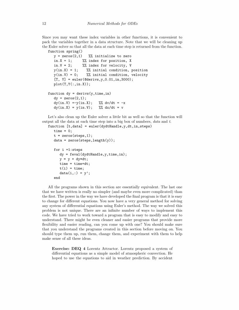
Since you may want these index variables in other functions, it is convenient topack the variables together in a data structure. Note that we will be cleaning upthe Euler solver so that all the data at each time step is returned from the function.

function spring()

y = zeros(2,1) %% initialize to zero

in.X = 1; %% index for position, X

in.V = 2; %% index for velocity, V

y(in.X) = 1; %% initial condition, position

y(in.V) = 0; %% initial condition, velocity

[T, Y] = euler(@derivs,y,0.01,in,3000);

plot(T,Y(:,in.X));

function dy = derivs(y,time,in)

dy = zeros(2,1);

dy(in.V) =-y(in.X); %% dv/dt = -x

dy(in.X) = y(in.V); %% dx/dt = v

Let’s also clean up the Euler solver a little bit as well so that the function willoutput all the data at each time step into a big box of numbers, data and t.

function [t,data] = euler(dydtHandle,y,dt,in,steps)

time = 0;

t = zeros(steps,1);

data = zeros(steps,length(y));

for i =1:steps

dy = feval(dydtHandle,y,time,in);

y = y + dy*dt;

time = time+dt;

t(i) = time;

data(i,:) = y’;

end

All the programs shown in this section are essentially equivalent. The last onethat we have written is really no simpler (and maybe even more complicated) thanthe first. The power in the way we have developed the final program is that it is easyto change for different equations. You now have a very general method for solvingany system of differential equations using Euler’s method. The way we solved thisproblem is not unique. There are an infinite number of ways to implement thiscode. We have tried to work toward a program that is easy to modify and easy tounderstand. There might be even cleaner and easier programs that provide moreflexibility and easier reading, can you come up with one? You should make surethat you understand the programs created in this section before moving on. Youshould type them up, run them, change them, and experiment with them to helpmake sense of all these ideas.

Exercise: DEQ 4 Lorentz Attractor. Lorentz proposed a system ofdifferential equations as a simple model of atmospheric convection. Hehoped to use the equations to aid in weather prediction. By accident


−20 −15 −10 −5 0 5 10 15 20 25 300

5

10

15

20

25

30

35

40

45

X

Z

Figure 7. Plot of X vs. Z produces the Lorentz ’butterfly’

he noticed that he when he solved his equations numerically, he gotcompletely different answers for only a small change in initial condition.He also noticed that while the variables plotted as a function of timeseemed random, the variables plotted against each other showed regularpatterns. You will use your Euler solver to reproduce some of Lorentz’sresults. The equations Lorentz derived were:

dx

dt= 10(y − x) (6.6)

dy

dt= x(20− z)− y (6.7)

dz

dt= xy −

8

3z (6.8)

We will not discuss the derivation of these equations but they werebased on physical arguments relating to atmospheric convection. Thevariables x, y, z represent physical quantities such as temperatures andflow velocities, while the numbers 10, 20, and 8/3 represent propertiesof the air.

Code up these equations using your Euler solver and explore their be-havior. Plot the time series for the variable X for an arbitrary initialcondition. Save the plot and show the behavior for a slightly changed(1 %) initial condition. Plot the variable x vs. z. You will know you areon the right track if that plot looks like Figure 7. Adjust the time stepand see if the solution is converging.

7. Error Estimates: Local Error

Let us return to the Taylor series approximation and use it to estimate the error inthe approximation to the derivative. If we assume that we have all the data (f and


it’s derivatives) at t=0, then the value of the function at time t = ∆t is given as

f(∆t) = f(t = 0) + ∆tdf

dt

∣

∣

∣

∣

t=0

+∆t2

2

d2f

dt2

∣

∣

∣

∣

t=0

+∆t3

6

d3f

dt3

∣

∣

∣

∣

t=0

+ ...∆tn

n!

dnf

dtn

∣

∣

∣

∣

t=0(7.1)

Rearranging this equation yields,

f(∆t)− f(t = 0)

∆t=

df

dt

∣

∣

∣

∣

t=0

+∆t

2

d2f

dt2

∣

∣

∣

∣

t=0

+∆t2

6

d3f

dt3

∣

∣

∣

∣

t=0

+...∆tn−1

n!

dnf

dtn

∣

∣

∣

∣

t=0

(7.2)

Since ∆t is small then the series of terms on the right hand side is dominated bythe term with the smallest power of ∆t, i.e.

f(∆t)− f(t = 0)

∆t=

df

dt

∣

∣

∣

∣

t=0

+∆t

2

d2f

dt2

∣

∣

∣

∣

t=0

+ ... (7.3)

Therefore, the Euler approximation to the derivative is off by a factor proportionalto ∆t. The good news is that the error goes to zero as smaller and smaller timesteps are taken. The bad news is that we need to take very small time steps to getgood answers. In the next section we will see that obtaining better accuracy doesnot require much extra work.

We call the error in the approximation to the derivative over one time step thelocal truncation error. This error occurs over one time step and can be estimatedfrom the Taylor series, as we have just shown.

Exercise: DEQ 5 Write a MATLAB program to solve

dy

dt= y (7.4)

using Euler’s method. Use the initial condition that y(t = 0) = 1, andsolve on the interval 0 < t < 1. The exact solution to this equation isy(t) = et. Try solving with a time step of 0.25, 0.1, 0.05, and 0.01. Plotthe error between the numerical solution and the analytical solution(y = et) as a function of ∆t. The result you should obtain is shown inFigure 8. Can you explain why the departure between the actual andpredicted error grows at large ∆t.

Let’s return to our original problem of the spring and see if we can understandwhy the first method that we tried worked so much better than the true Eulermethod in equation 5. If you recall the first implementation worked quite wellbecause it was not a true Euler method. The first algorithm that we tried can bewritten as

xN+1 = xN + vN∆t (7.5)

vN+1 = vN − kxN+1∆t (7.6)

Advancing to the next time step the equation for x becomes

xN+2 = xN+1 + vN+1∆t (7.7)


10−2

10−1

10−2

10−1

∆ t

Err

or

Figure 8. Error as the time step is changed for Euler’s method applied to dy/dt = y. Boththe error and the function error = ∆t/2 are plotted. One can see from Equation 7.3, thatthe error in the approximation is just as predicted, with slight departure for large timesteps. Note that we are plotting the difference between the true and numerical solution att = 1.

which can be rewritten as

xN+2 = xN + vN∆t+∆t(vN − k∆t(xN + vN∆t)). (7.8)

Collecting terms we obtain

xN+2 = xN + vN2∆t− kxN∆t2 − k∆t3vN∆t. (7.9)

using the fact that −kxN = d2x/dt2 and vN = dx/dt we can write the expressionfor xN+2 as

xN+2 = xN + 2∆tdx

dt

N

+∆t2d2x

dt2

N

+∆t3d3x

dt3

N

. (7.10)

The first 3 terms on the right hand side of this equation are the Taylor series forthe point xN+2: the ∆t3 term does not cancel. If we expand the velocity we willfind the same result. This method is formally accurate to terms of order ∆t2 ratherthan ∆t of the true Euler method. The method that was the easiest to program,in this case turned out to be a good one. Unfortunately, in general the easier themethod the less accurate!

8. Error Estimates: Global Error

In the last section we looked at how the error changed as we varied the step size. Wealso used the Taylor series to estimate the discretization error associated with thescheme that we were using. In addition to error at each time step, there is a globalerror associated with the accumulation of errors at each time step. Refer back to thespring problem and our attempt to apply the Euler method to the motion, Figure6. It is clear that in this case the error is accumulating. If we look at the results


0 5 10 15 20 25 30−0.5

−0.4

−0.3

−0.2

−0.1

0

0.1

0.2

0.3

0.4

0.5

time

Err

or

Figure 9. Error between numerical and true solution as a function of time for the mass onspring system. The straight line shows t∆t/2. We see that the error is primarily a simplesum of the truncation error at each time step. The non-linear behavior seen in the erroris due to the fact that the error depends on the solution, i.e. at long times the error willgrow exponentially.

for one cycle of the oscillation with the large step size we might think that thesolution has some error, but we might think that error is acceptable - it seems thatthe position is off by 10%. At the end of 4 oscillations the large step size is clearlygiving results that are not acceptable. Physically we know that the system shouldconserve energy and clearly the numerical solution is artificially gaining energy. Theaccumulation of error is known as global error.

In Figure 9 we show the global error (yn − yexact(tn)) as a function of time forthe mass-spring system. We find that the global error of the numerical approxi-mation is well estimated by the simple sum of the local truncation errors. We findthat the situation is somewhat worse since the local truncation error depends onthe second derivative of the function itself (see equation 7.3). Therefore, as theerror accumulates and the solution grows, even more error is introduced into theapproximation. At long times we find exponential growth of the error. It is clearthat accumulation of global error can be a severe problem for Euler’s method.

Now that we have discussed the impact of numerical truncation error we willbegin to look at schemes that are designed to be more accurate.

9. Midpoint method

When numerically solving differential equations, we want to find the best estimatefor the ’effective slope’ across the time step interval. So far we have used the valueof the slope at the start of the interval since this is the only location where we haveany information about the function. Consider figure 10 where we have plotted thefunction f(t) = et and various approximations for the derivative to shoot acrossthe interval 0 < t < 1. We clearly see that the simple Euler method shoots too low.If we somehow knew the value at the endpoint of the shooting interval (t = 1) and


0 0.5 1 1.5 21

2

3

4

5

6

7

8

time

F(t

)

1 + x

1 + x e0.5

1 + x e1

Figure 10. Midpoint approximation for f(t) = et

used that value, we would shoot too high. If we conjecture that using a value fromthe midpoint of the interval might be better representation of the effective slope ofacross the interval, we get a much better answer. The reason why can be derivedquite easily (and seen in Figure 10). The approximation that looks good in thisfigure is

f(∆t) = f(t = 0) + ∆tdf

dt

∣

∣

∣

∣

t=∆t/2

(9.1)

Expanding the derivative of f with respect to time using a Taylor series yields

df

dt

∣

∣

∣

∣

t=∆t/2

=df

dt

∣

∣

∣

∣

t=0

+∆t

2

d2f

dt2

∣

∣

∣

∣

t=0

+∆t2

4

d3f

dt3

∣

∣

∣

∣

t=0

+ ... (9.2)

Substituting this expression into equation 9.1 yields

f(∆t) = f(t = 0) + ∆t

(

df

dt

∣

∣

∣

∣

t=0

+∆t

2

d2f

dt2

∣

∣

∣

∣

t=0

+∆t2

4

d3f

dt3

∣

∣

∣

∣

t=0

+ ...

)

(9.3)

We see that the first three terms of the right-hand-side exactly match the Taylorseries approximation. Therefore the error of the approximation is on the order of∆t2. The problem with this method is that this method requires knowing data inthe future. The problem can be remedied with a simple approximation, we willuse the Euler method to shoot to an approximated midpoint. We will estimate thederivative there and then use the result to make the complete step. Specifically, themidpoint method works as follows.

yN+1/2 = yN +∆t

2

dy

dt

N

(9.4)

yN+1 = yN +∆tdy

dt

N+1/2

. (9.5)


0 0.2 0.4 0.6 0.8 11

1.2

1.4

1.6

1.8

2

2.2

2.4

2.6

2.8

Euler step across half interval, yN+1/2 = 1+0.5

Step across interval, yN+1 = 1 + (1+0.5)

Exact Solution

time

Y(t

)

Figure 11. Example of the midpoint method for y(t) = et, where ∆t = 1. First we take anEuler step to the midpoint of the interval. The ’effective slope’ for the interval is computedat this approximate midpoint location. The midpoint slope is used to take the full stepacross the interval.

The first step applies Euler’s method halfway across the interval. The values ofyN+1/2 and t = ∆t/2 are used to recompute the derivatives. The values of theestimated midpoint derivatives are then used to shoot across the entire domain. Aschematic is shown in Figure 11 for the equation dy/dt = y using a large time stepof ∆t = 1 in order to amplify the effects. The initial condition is y(t = 0) = 1, sotherefore dy/dt0 = 1 via the governing equation. Applying the governing equationand the initial condition

yN+1/2 = 1 + 1∆t/2 (9.6)

yN+1 = 1 +∆t(1 + ∆t/2) (9.7)

Exercise: DEQ 6 Write a MATLAB program similar to the Eulersolver that applies the midpoint method. The program should be generalso that you can apply it to any system of equations. The program shouldalso follow the same usage as the Euler solver so that in your programsyou could easily switch between methods.

Use your midpoint solver to solve your mass-spring system. Comparethe result to the Euler solver. Change the time step and assess the errorof the approximation by comparing to the exact solution.

10. Runge-Kutta Method

There are many, many, many different schemes for solving ODEs numerically. Someof them exist for a good reason, some are never used, some were relevant when com-puters were slow, some just aren’t very good. However, different types of equationsare better suited for different methods, we will discuss this more in the next section.The basic ideas, however are similar to the ones that we have already presented: the


schemes try to minimize the amount of error in estimating the slope that propagatesthe solution forward.

One of the standard workhorses for solving ODEs is the called the Runge-Kutta method. This method is simply a higher order approximation to the midpointmethod. Instead of shooting to the midpoint, estimating the derivative, the shootingacross the entire interval - the Runge-Kutta method takes four steps, shooting acrossone quarter of the interval, estimating the derivative, then shooting to the midpoint,and so on. We will not provide a formal derivation of the Runge-Kutta algorithm,instead we will present the method and implement it.

The general ODE that we are solving is given as,

dy

dt= f(y, t). (10.1)

The Runge-Kutta method can be defined as:

k1 = ∆tf(tN , yN ) (10.2)

k2 = ∆tf(tN +∆t/2, yN + k1/2) (10.3)

k3 = ∆tf(tN +∆t/2, yN + k2/2) (10.4)

k4 = ∆tf(tN +∆t, yN + k3) (10.5)

yN+1 = yN +k1

6+k2

3+k3

3+k4

6(10.6)

One should note the similarity to the midpoint method discussed in the previoussection. Also note that each time step requires 4 evaluations of the derivatives, i.e.the function f.

Since we have only given the equations to implement the Runge-Kutta methodit is not clear how the error behaves. Rather than perform the analysis, we willcompute the error by solving an equation numerically and compare the result toan exact solution as we vary the time step. To test the error we solve the modelproblem, dy/dt = −y, where y(0) = 1 and we integrate until time t = 1. In Figure12 we plot the error between the exact and numerical solutions at t = 1 as a functionof the time step size. We also plot a function f = C∆t4 on the same graph. Wefind that the error of the Runge-Kutta method scales as ∆t4. This is quite good -if we double the resolution (half the time step size) we get 16 times less error!.

Exercise: DEQ 7 Implement the Runge-Kutta method by writing afunction that works in the same way as your midpoint method and Eulersolvers, only using this new algorithm.

Use your Runge-Kutta solver to solve your mass-spring system. Com-pare the result to the Euler and midpoint solver. Compare the Runge-Kutta solution to the exact solution and plot the error on a log-logplot as you vary the time step size. How does this plot compare to onegenerated applying the midpoint method?


10−2

10−1

100

10−12

10−10

10−8

10−6

10−4

10−2

∆ t

erro

r

~∆ t4

Figure 12. The error between the Runge-Kutta method and exact solution as a functionof time step size. One the plot we also display a function that scales as ∆t4. We see thatthis fits the slop of the data quite well, therefore error in the Runge-Kutta approximationscales as ∆t4.

11. Stability and Stiff Equations: Backward Euler Method

So far we have only discussed accuracy of ODE solvers, but another importantissue is stability. In many situations we find that the algorithms we have thus fardiscussed will be unstable unless the time step is very small. By unstable, we meanthe solution will begin to oscillate or grow in an unphysical manner.

Consider the following set of coupled ODEs:

dy

dt= −100(x+ y) (11.1)

dx

dt= −x (11.2)

Equations of this form are common in chemistry where x and y are chemical speciesand the coefficients in the equation (100 & 1) are reaction rates. It is common inchemical systems to have reactions with varying rates of progress. Stiff equationsare have widely different time scales that can cause a numerical solution difficultyeven though the ’fast’ time scale might not be important for the final solution.

Exercise: DEQ 8 Set up equations 11.1 and 11.2 using your Eulersolver and the initial conditions that x(t = 0) = y(t = 0) = 1. Set yourtime step to 0.001 and take 2000 time steps. Plot the x(t) and y(t) onthe same graph.

If you completed the exercise then you should generate a plot that looks likeFigure 13. This behavior is very common in chemical systems, notice that one chem-ical (Y) goes from +1 to -1 very rapidly, then undergoes a much slower increased.The behavior is indicative of the two times scales present in the equations, 1/100and 1.


0 0.5 1 1.5 2−1

−0.8

−0.6

−0.4

−0.2

0

0.2

0.4

0.6

0.8

1

time

Y(t

), X

(t)

Figure 13. Solution to the stiff differential equations 11.1 and 11.2. Note the two timescales in the solution for y, there is the rapid decrease followed by the slow convergenceto zero.

Exercise: DEQ 9 Set up equations 11.1 and 11.2 using your Eulersolver and the initial conditions that x(t = 0) = 1, y(t = 0) = −1. Setyour time step to 0.001 and take 2000 time steps. Plot the x(t) and y(t)on the same graph.

After completing this exercise you should notice that the plot looks very similarto Figure 13, only the observation of the fast time scale is not present. In this casewe have set the initial condition such that the fast time scale does not influence theappearance of the solution to the equations. The fast time scale does influence thenumerical solution, however. Try the following exercise:

Exercise: DEQ 10 Set up equations 11.1 and 11.2 using your Eulersolver and the initial conditions that x(t = 0) = 1, y(t = 0) = −1. Setyour time step to 0.02001 and take 2000 time steps. Plot the x(t) andy(t) on the same graph.

Once you complete this exercise you should obtain a plot that looks like Figure14. The solution looks correct at early times, but then we find that the solution ofy begins to oscillate across zero after the solution has come close to its final steadystate solution of x = y = 0. The numerical solution is unstable. Try making ∆t justa little bit larger and you will notice that the solution is wildly unstable.

So what has happened, why has the solution gone unstable? A simple wayto view stability is consider the Euler method applied to the equation dy/dt =−Cy, y(t = 0) = 1. When we write out Euler’s method for this equation we obtain

yN+1 = (1− C∆t)yN . (11.3)

We know that the true solution of this ODE should decay from 1 to 0 on a timescale of 1/C. It is easy to see that if C∆t < 1 then the iterative equation 11.3


0 5 10 15 20 25 30 35 40 45−1

−0.8

−0.6

−0.4

−0.2

0

0.2

0.4

0.6

0.8

1

time

Y(t

), X

(t)

Figure 14. Solution to stiff equations showing unstable behavior.

has qualitatively the right behavior, each subsequent value of y is smaller than thelast. If C∆t > 1 then we see that the sign of y will change with each iteration,i.e. the equations are behaving in a non-physical manner. Further, if C∆t > 2then y will approach infinity as the number of iterations approaches infinity; eachsubsequent value of y is greater than the last. This stability problem is essentiallywhat has happened in our example of the the two coupled equations. The stabilityrequirements say that the equations must be integrated with the shortest timescale, regardless if that time scale is influencing the solution. This can be a seriouslimitation in many situations even on modern computers. In chemistry applicationsone often cares about the reactions that occur over several seconds where the fastesttime scale in the system might be a few nano-seconds. It would require 109 timesteps to solve this system, a lot of work even for a fast PC.

Fortunately methods exist for solving stiff equations. A very simple way tomake a system more stable is to use the Backward Euler method. This method usesinformation from the end of the time step interval to estimate the derivative, i.e.

yN+1 = yN +dy

dt

N+1

(11.4)

Applying the Backward Euler technique to the equation dy/dt = −Cy, y(t = 0) = 1yields,

yN+1 =yN

(1 + C∆t). (11.5)

It is easy to see from this equation that regardless of the time step size the systemwill always display the correct behavior: subsequent values of y will always besmaller than the last, and y will never go negative. Of course stability does notmean accuracy.

The difficulty with Backward Euler solvers is that they require information fromthe future and are therefore often more difficult (or impossible) to implement fornon-linear equations. However, for linear equations such as the simple system thatwe are dealing with in this section it is quite easy to implement the method directly.


Exercise: DEQ 11 Solve equations 11.1 and 11.2 using a BackwardEuler method with the initial conditions x(t = 0) = 1, y(t = 0) =−1. You do not need to write a general Backward Euler solver, justimplement a method specific for these equations. Set your time step to0.25 and take 40 time steps. Plot the x(t) and y(t) on the same graph.You should obtain a solution that looks quite reasonable. Notice thatyou can obtain the same solution at a fraction of the cost of the forwardEuler.

There are a variety semi-implicit methods that are effective for solving stiffsystems in both linear and non-linear equations. These semi-implicit methods arevery important in the solution of ODEs but we will not cover them in this class.

12. Using MATLAB

As mentioned previously, the backward Euler method is not convenient as a generalmethod since the discretized equations and ability to apply the method depend onthe problem that you are solving. Many general methods exist for stiff equations,but they are all based on the general idea of the backward Euler method, usinginformation from the future tends to stabilize the numerical method.

At this point it is worth introducing the ODE solvers that are built into MAT-LAB. These solvers are very general, employ adaptive time stepping (speed up orslow down when it needs to), and have the capability for handling stiff equations.So you ask, if MATLAB can do all this already then why did you make us write allthese programs? Well, it is very easy to employ packaged numerical techniques andobtain bad answers, especially in complex problems. It is also easy to use a packagethat works just fine, but the operator (i.e. you) makes a mistake and gets a badanswer. It is important to understand some of the basic issues of ODE solvers sothat you will be able to use them correctly and intelligently. On the other hand, ifother people have already spent a lot of time developing sophisticated techniquesthat work really well, why should we replicate all their work. We turn to these’canned’ routines at this point.

You have already developed a your own Runge-Kutta solver. MATLAB has asolver that is called ODE45 and the usage of the function will be very similar to theroutines that you wrote for the Euler method, midpoint method, and Runge-Kutta.The ODE45 command uses the same Runge-Kutta algorithm you developed, onlythe MATLAB version uses adaptive time stepping. At this point in this tutorial weare going to let you figure out how to use the ODE45 command. You can read thehelp (i.e. type help ode45), though that isn’t the best help out there. You can alsosurf the MATLAB web page documentation and find some examples of using theODE45 routine.

As mentioned, the ode45 command uses adaptive step sizes to control the error.With these algorithms you specify the error (there is a default) and the algorithmadjusts the time step size to maintain this at a constant level. Therefore, withadaptive algorithms you cannot generate a plot of error vs. time step size. In generalthese adaptive algorithms work by comparing the difference between taking a stepwith two methods that have different orders (i.e. midpoint (∆t2) and Runge-Kutta


(∆t4)). The difference is indicative of the error, and the time step is adjusted(increased or decreased) to hold the error constant.

Exercise: DEQ 12 Through the MATLAB documentation, figure outhow to use the ode45 command. Apply the ODE45 command to thespring equations that we discussed in previous sections. Compare theresults to those obtained with Euler, Midpoint, and Runge-Kutta solver.Compare the error between the true and numerical solutions. Try toadjust the error tolerance on the ODE45 command and see that thetolerance and the true error roughly agree.

MATLAB has other ODE solvers in addition to the ODE45. You can readthe help on the MATLAB web page about the different solvers. The two mostcommon that you will use are ode45 and ode23s. ODE23s is optimized for solvingstiff equations. Try the following exercise to really see the difference.

Exercise: DEQ 13 Apply the ODE45 and ODE23s command to equa-tions 11.1 and 11.2. Compare the results obtained with both methods,specifically note how many time steps each method took. Compare thedifference between the two methods for the same error tolerance.

13. Is your solution correct?

One of the big difficulties in using numerical methods is that takes very little timeto get an answer, it takes much longer to decide if it is right. Usually the first test isto check that the system is behaving physically. Usually before running simulationsit is best to use physics to try and understand qualitatively what you think yoursystem will do. Will it oscillate, will it grow, will it decay? Do you expect yoursolution to be bounded, i.e. if you start a pendulum swinging under free gravityyou would not expect that the height of the swing would grow.

We already encountered unphysical growth when we solved the mass-springmotion using Euler’s method in Figure 5 and 6. When the time step was large wenoticed unphysical behavior: the amplitude of the mass on the spring was growingwith time. This growth in oscillation amplitude is violating the conservation ofenergy principle, therefore we know that something is wrong.

One simple test of a numerical method is to change the time step and see whathappens. If you have implemented the method correctly (and its a good method)the answer should converge as the time step is decreased. If you know the orderof your approximation then you know how fast this decrease should happen. If themethod has an error proportional to ∆t then you know that cutting the time stepin half should cut the error in half. You should NEVER NEVER turn in resultsfrom a simulation where you do not check different time steps to make sure thatyour solution is converging. You should also note that just because the solutionconverges does not mean that your answer is correct.

The MATLAB routines use adaptive time stepping, therefore you should varythe error tolerance rather than the time step interval. You should always check theconvergence as you vary the error. Plot the difference between subsequent solu-tions as you vary the error tolerance. Further results on checking convergence andexamples of doing so will be given in the problem example supplement.


References

Boyce & DiPrima, 2001 Elementary Differential Equations and Boundary Value Problems,John Wiley and Sons. (This is your Math text).

Epperson, 2002 An Introduction to Numerical Methods and Analysis John Wiley andSonce.

Press, Tuekolsky, Vetterling, & Flannery, 1992 Numerical Recipes in C, Cambridge Uni-versity Press. See www.nr.com for free pdf version.

MATLAB Product Documentation www.mathworks.com.

NumericalMethodsforOrdinary … reason for rewriting the equations as a system of two coupled...

Documents

Transcript of NumericalMethodsforOrdinary … reason for rewriting the equations as a system of two coupled...