NUMERICAL STUDY OF VOLTERRA DIFFERENCE EQUATIONS OF … · 2018-03-14 · NUMERICAL STUDY OF...
119
NUMERICAL STUDY OF VOLTERRA DIFFERENCE EQUATIONS OF THE SECOND KIND By Said Ali Al-Garni A Thesis Presented to the DEANSHIP OF GRADUATE STUDIES In Partial Fullfillment of the Requirements for the degree Master of Science IN Mathematical Sciences KING FAHD UNIVERSITY OF PETROLEUM & MINERALS Dhahran, Saudi Arabia April, 2003
Transcript of NUMERICAL STUDY OF VOLTERRA DIFFERENCE EQUATIONS OF … · 2018-03-14 · NUMERICAL STUDY OF...
NUMERICAL STUDY OFVOLTERRA DIFFERENCE
EQUATIONS OF THE SECONDKIND
By
Said Ali Al-Garni
A Thesis Presented to theDEANSHIP OF GRADUATE STUDIES
In Partial Fullfillment of the Requirementsfor the degree
Master of ScienceIN
Mathematical Sciences
KING FAHD UNIVERSITYOF PETROLEUM & MINERALS
Dhahran, Saudi Arabia
April, 2003
KING FAHD UNVERSITY OF PETROLEUM & MINERALSDHAHRAN 31261, SAUDI ARABIA
DEANSHIP OF GRADUATE STUDIES
This thesis, written by Said Ali Al-Garni under the direction of his thesisadvisor and approved by his thesis committee, has been presented to and acceptedby the Dean of Graduate Studies, in partial fulfillment of the requirements of thedegree of MASTER OF SCIENCE IN MATHEMATICS.
Thesis Committee
Dr. Haydar Akca, Thesis Advisor
Dr. Basem Attili, Member
Dr. Abdulaziz Al-Shuaibi, Member
Dr. Khaled FuratiDepartment Chairman
Prof. Osama JannadiDean of Graduate Studies
Date
.
DedicationI wish to dedicate this thesis to my parents,
my brothers, my sisters, my wife, my kids andmy friends
iii

Acknowledgment
First of all I thank ”ALLAH” The Almighty for the knowledge, help and guidance
HE has showered on me. Thanks are also to our Prophet Mohammad (pbuh) who
encouraged us as Muslims to seek knowledge and stressed that science and Islam are
never separable.
My sincere appreciations are due to Prof. Hydar Akca, my main advisor, for his
help, support and encouragement in making this work possible. I am sincerely grate-
ful to my thesis members, Dr. Basem Attili and Dr. Abdulaziz Al-Shuaibi for their
helpful comments.
Acknowledgments are due to King Fahd University of Petroleum and Minerals for
giving me the opportunity to pursue my study. A special thank is due to Prof. Ali
Al-Daffa’ and Prof Mohammad Al-Bar for their support and help.
My sincere appreciation are due to Dr. Salim Masoudi, my academic advisor, Dr.
Khaled Furati, chairman, and all other faculty of the department of mathematical
sciences for their concern and encouragement.
Last but not least, I put in record myhigh appreciation to the support of my parents,
my brothers, my sisters, my wife, and my kids, Mohammad and Raghd, during the
study period.
iv
Contents
Dedication iii
Acknowledgment iv
List of Tables vii
Thesis Abstract viii
Arabic Abstract ix
Preface 1
1 Linear Difference Equations 31.1 Linear First Order Difference Equations . . . . . . . . . . . . . . . . 51.2 Linear Difference Equations of Higher Order . . . . . . . . . . . . . . 61.3 Linear Homogeneous Equations with Constant Coefficients . . . . . . 81.4 Linear Nonhomogeneous Equations . . . . . . . . . . . . . . . . . . . 91.5 Systems of Difference Equations . . . . . . . . . . . . . . . . . . . . . 101.6 Stability Theory . . . . . . . . . . . . . . . . . . . . . . . . . . . . . . 141.7 Liapunov′s Direct or Second Method . . . . . . . . . . . . . . . . . . 171.8 Z - Transform Method . . . . . . . . . . . . . . . . . . . . . . . . . . 19
2 Volterra Difference Equations 222.1 The Scalar Case of Volterra Difference Equations of Convolution Type 232.2 Equations of Nonconvolution Type . . . . . . . . . . . . . . . . . . . 282.3 Equations of Convolution Type . . . . . . . . . . . . . . . . . . . . . 342.4 A Criterion for Uniform Asymptotic Stability . . . . . . . . . . . . . 372.5 Boundedness of Solutions of Volterra Equations . . . . . . . . . . . . 412.6 Volterra Difference Equations with Degenerate Kernels . . . . . . . . 492.7 Nonlinear Volterra Difference Equations . . . . . . . . . . . . . . . . 57
v
3 Discretization of Volterra Equations 623.1 Discretization of Volterra Integral and Integro-differential Equations . 62
3.1.1 Existence and Uniqueness of the Solution . . . . . . . . . . . . 643.1.2 Boundedness of the Direct Quadrature Method . . . . . . . . 67
3.2 Discretization of Volterra Integral and Integro-differential EquationsUsing Linear Multistep Methods . . . . . . . . . . . . . . . . . . . . . 743.2.1 Applying the Linear Multistep Method . . . . . . . . . . . . . 753.2.2 Construction of Quadrature Rules . . . . . . . . . . . . . . . . 79
4 Estimation of Solutions of Volterra Equations 82
4.1 Estimation of Solutions of Linear Volterra Equations . . . . . . . . . 824.2 Estimation of Solutions of Nonlinear Volterra Equations . . . . . . . 87
5 Conclusion and Further Research 96
Appendices 98
A A program for solving VIE 98
B A program for solving VIDE 1 102
C A program for solving VIDE 2 104
References 106
Vita 110
vi
List of Tables
3.1 Results of Example 3.1.1 . . . . . . . . . . . . . . . . . . . . . . . . . 703.2 Results of Example 3.1.2 with Trapezoidal’s weights . . . . . . . . . . 733.3 Results of Example 3.1.2 with Simpson’s weights . . . . . . . . . . . . 74
vii
Thesis Abstract
Full Name Of Student : Said Ali Al-Garni
Title Of Study : Numerical Study of Volterra Difference
Equations of the Second Kind
Major Field : Mathematics
Date Of Degree : April 2003
In this thesis, we will consider Volterra difference equations of the second kind.
Three different kernels, nonconvolution, convolution and degenerate , are introduced.
Boundedness, periodicity, and stability are among the most properties of Volterra
difference equations discussed. We consider discretization of Volterra integral and
integro-differential equations using numerical methods. Specific programs are con-
structed to solve these equations using numerical methods. Finally, we give estima-
tions of solutions of both linear and nonlinear Volterra difference equations.
viii

ix
Preface
Volterra difference equations, whose solution is defined by the whole previous his-
tory, are widely used in the modeling of the processes in so many fields. In addition
to networks, Volterra equation has been successfully applied to specific problems in
such areas as communication, fluid mechanics, biophysics, optics, biomedical model-
ing, ecology (population dynamics), naval architecture, solid state, device modeling,
problem of control, biomechanics, combinatorics, epidemics and some schemes of nu-
merical solutions of integral and intgro-differential equations.
The work is organized as follows. Chapter 1 introduces the relevant basic defini-
tions and notations that are commonly used for linear difference equations. In ad-
dition, some needed results are presented. Chapter 2 introduces Volterra difference
equations. The scalar case, equations of nonconvolution, equations of convolution
and equations of degenerate kernels are considered. Also, boundedness, periodicity,
and stability are among the most properties of Volterra difference equations will be
discussed. Moreover, Chapter 2 includes some results of the nonlinear case. Next,
in Chapter 3, we consider discretization of Volterra integral and integro-differential
equations using numerical methods such as backward Euler, trapezoidal and linear
multistep methods. Specific programs are provided to solve these equations using
1

2
numerical methods. Finally, in Chapter 4, we discuss estimations of solutions of both
linear and nonlinear Volterra difference equations.
Chapter 1
Linear Difference Equations
Mathematical computions frequently are based on equations that allow us to com-
pute the value of a function recursively from a given set of values. Such equations
are called “difference equations”. These equations occur in numerous settings and
forms, both in mathematics itself and in its applications to statistics, computing,
electrical circuit analysis, dynamical systems, economics, biology, and other fields.
For example, if a certain population has discrete generations, the relation expresses
itself in the difference equation
x(n + 1) = f(x(n)), (1.1)
where x(n) is the size of population at the n the stage and one may consider n is a
year. We may use this example to introduce some notations. Starting from a point
x0 , one may generate the sequence
x0, f(x0), f(f(x0)), f(f(f(x0))), .... (1.2)
= x0, f(x0), f 2(x0), f 3(x0), ...
= x0, x1, x2, x3, ....
This iterative procedure is an example of a discrete dynamical system. Letting
3
Chapter 1. Linear Difference Equations 4
x(n) = fn(x0), we have
x(n + 1) = fn+1(x0) = f [fn(x0)] = f(x(n)).
Observe that x(0) = f 0(x0) = x0. If the function f in (1.1) is replaced by a function
g of two variables, that is g : Z+×R → R , where Z+ is the set of positive integers
and R is the set of real numbers, then we have
x(n + 1) = g(n, x(n)). (1.3)
Equation (1.3) is called nonautonomous or time-variant whereas (1.1) is called
autonomous or time-invariant. If an initial condition x(n0) = x0 is given, then
for n ≥ n0 there is a unique solution x(n) = x(n, n0, x0) of (1.3) such that
x(n0, n0, x0) = x0. This may be shown easily by iteration
x(n0 + 1, n0, x0) = g(n0, x(n0)) = g(n0, x0);
x(n0 + 2, n0, x0) = g(n0 + 1, x(n0 + 1)) = g(n0 + 1, f(n0, x0));
x(n0 + 3, n0, x0) = g(n0 + 2, x(n0 + 2)) = g[n0 + 2, f(n0 + 1, f(n0,x0))].
And inductively we get
x(n, n0, x0) = g[n− 1, x(n− 1, n0, x0)].
Chapter 1. Linear Difference Equations 5
1.1 Linear First Order Difference Equations
A typical linear homogeneous first-order equation is given by
x(n + 1) = a(n)x(n), x(n0) = x0 for n ≥ n0, (1.4)
and the associated nonhomogeneous equation given by
y(n + 1) = a(n)y(n) + g(n), y(n0) = y0 for n ≥ n0 ≥ 0, (1.5)
where in both equations, it is assumed that a(n) 6= 0 , a(n), and g(n) are real-
valued functions defined for n ≥ n0 ≥ 0. One may find the solution of (1.4) by simple
iteration.
Definition 1.1.1 A point x∗ in the domain of f is said to be an equilibrium point of
(1.1) if it is a fixed point of f, i.e., f(x∗) = x∗.
Definition 1.1.2
(i) The equilibrium point x∗ of (1.1) is stable if given ε > 0 there exists δ > 0 such
that |x0 − x∗| < δ implies |fn(x0)− x∗| < ε for all n > 0 . If x∗ is not stable, then
it is called unstable.
(ii) The point x∗ is an asymptotically stable (attracting)equilibrium point if it is
stable and there exists η > 0 such that |x(0)− x∗| < η implies limn→∞
x(n) = x∗. If
η = ∞ , x∗ is said to be globally asymptotically stable.
Definition 1.1.3 Let b be in the domain of f Then;
(i) b is called a periodic point of (1.1) if for some positive integer k, fk(b) = b . Hence
a point is k-periodic if it is a fixed point of fk , that is, if it is an equilibrium point
Chapter 1. Linear Difference Equations 6
of the difference equation
x(n + 1) = g(x(n)), (1.6)
where g = fk;
(ii) b is called eventually k periodic if for some positive integer m, fm(b) is a k
periodic point. In other words, b is eventually k-periodic if fm+k(b) = fm(b) .
1.2 Linear Difference Equations of Higher Order
The normal form of a k th-order nonhomogeneous linear difference equation is given
by
y(n + k) + p1(n)y(n + k − 1) + · · ·+ pk(n)y(n) = g(n) , (1.7)
where pi(n) and g(n) are real valued functions defined for n ≥ n0 and pk(n) 6= 0 for
all n ≥ n0 . If g(n) is identically zero then (1.7) is said to be a homogeneous equation.
By letting n = 0 in (1.7), we obtain y(k) in terms of y(k − 1), y(k − 2), ..., y(0).
Explicitly, we have
y(k) = −p1(0)y(k − 1)− p2(0)y(k − 2)− · · · − pky(0) + g(0).
Once y(k) is computed, we can find y(k + 1) . Repeating this process, it is possible
to evaluate all values of y(n) for n ≥ k.
A sequence y(n)∞n0or simply y(n) is said to be a solution of (1.7) if it satisfies
the equation. Observe that if we specify the initial data of the equation, we are led
to the corresponding initial value problem
y(n + k) + p1(n)y(n + k − 1) + · · ·+ pk(n)y(n) = g(n), (1.8)
Chapter 1. Linear Difference Equations 7
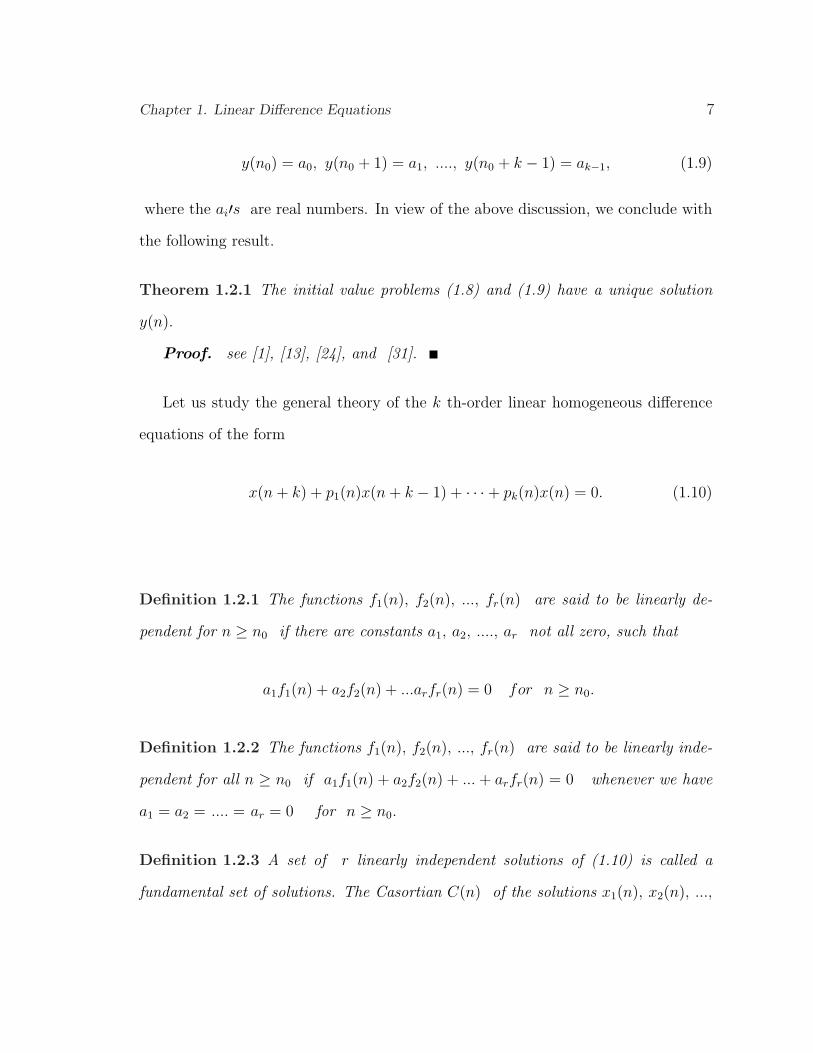
y(n0) = a0, y(n0 + 1) = a1, ...., y(n0 + k − 1) = ak−1, (1.9)
where the ai′s are real numbers. In view of the above discussion, we conclude with
the following result.
Theorem 1.2.1 The initial value problems (1.8) and (1.9) have a unique solution
y(n).
Proof. see [1], [13], [24], and [31].
Let us study the general theory of the k th-order linear homogeneous difference
equations of the form
x(n + k) + p1(n)x(n + k − 1) + · · ·+ pk(n)x(n) = 0. (1.10)
Definition 1.2.1 The functions f1(n), f2(n), ..., fr(n) are said to be linearly de-
pendent for n ≥ n0 if there are constants a1, a2, ...., ar not all zero, such that
a1f1(n) + a2f2(n) + ...arfr(n) = 0 for n ≥ n0.
Definition 1.2.2 The functions f1(n), f2(n), ..., fr(n) are said to be linearly inde-
pendent for all n ≥ n0 if a1f1(n) + a2f2(n) + ... + arfr(n) = 0 whenever we have
a1 = a2 = .... = ar = 0 for n ≥ n0.
Definition 1.2.3 A set of r linearly independent solutions of (1.10) is called a
fundamental set of solutions. The Casortian C(n) of the solutions x1(n), x2(n), ...,
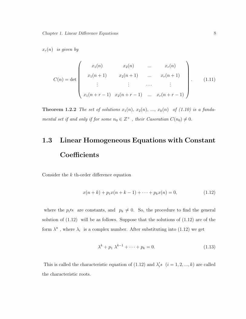
Chapter 1. Linear Difference Equations 8
xr(n) is given by
C(n) = det
x1(n) x2(n) ... xr(n)
x1(n + 1) x2(n + 1) ... xr(n + 1)
...... · · · ...
x1(n + r − 1) x2(n + r − 1) ... xr(n + r − 1)
. (1.11)
Theorem 1.2.2 The set of solutions x1(n), x2(n), ..., xk(n) of (1.10) is a funda-
mental set if and only if for some n0 ∈ Z+ , their Casoratian C(n0) 6= 0.
1.3 Linear Homogeneous Equations with Constant
Coefficients
Consider the k th-order difference equation
x(n + k) + p1x(n + k − 1) + · · ·+ pkx(n) = 0, (1.12)
where the pi′s are constants, and pk 6= 0. So, the procedure to find the general
solution of (1.12) will be as follows. Suppose that the solutions of (1.12) are of the
form λn , where λi is a complex number. After substituting into (1.12) we get
λk + p1 λk−1 + · · ·+ pk = 0. (1.13)
This is called the characteristic equation of (1.12) and λ′is (i = 1, 2, ..., k) are called
the characteristic roots.
Chapter 1. Linear Difference Equations 9
1.4 Linear Nonhomogeneous Equations
Consider (1.7) where pk(n) 6= 0 for all n ≥ n0 . The sequence g(n) is called the
forcing term, external force, the control, or input of the system.
Theorem 1.4.1 Any solution y(n) of (1.7) may be written as
y(n) = yp(n) +k∑
i=1
aixi(n),
where x1(n), x2(n), ..., xk(n) is a fundamental set of solutions of the homoge-
neous equation (1.10) and a solution of the nonhomogeneous equation (1.7) is called
a particular solution and denoted by yp(n). General solution of the nonhomogeneous
equation (1.7) as
y(n) = yc(n) + yp(n). (1.14)
To compute the particular solution yp(n) the method of undetermined coefficients
and variation of parameters are commonly using methods, see [1], [13], [24], and [31]
for different forms of g(n).
Example 1.4.1 Consider the following equation
y(n + 2) + y(n + 1)− 12y(n) = n2n.
The characteristic roots of the homogneous equation are λ1 = 3 and λ2 = −4. Hence,
yc(n) = c13n + c2(−4)n.
Chapter 1. Linear Difference Equations 10
And the particular solution
yp(n) = a12n + a2n2n.
Substituting this relation into our equation, we could find the values of a1 and a2.
Then the particular solution is
yp(n) =−5
182n − 1
6n2n,
and the general solution is
y(n) = c13n + c2(−4)n − 5
182n − 1
6n2n.
1.5 Systems of Difference Equations
Consider the following system of k linear first-order difference equations
x1(n + 1) = a11x1(n) + a12x2(n) + ... + a1kxk(n)
x2(n + 1) = a21x1(n) + a22x2(n) + ... + a2kxk(n)
...
xk(n + 1) = ak1x1(n) + ak2x2(n) + ... + akkxk(n)
. (1.15)
This system may be written in the vector form
x(n + 1) = Ax(n), (1.16)
where x(n) = (x1(n), x2(n), ..., xk(n))T ∈ Rk, and A = (aij) is a k× k real nonsin-
gular matrix. Since A does not depend on n so we called this system autonomous
Chapter 1. Linear Difference Equations 11
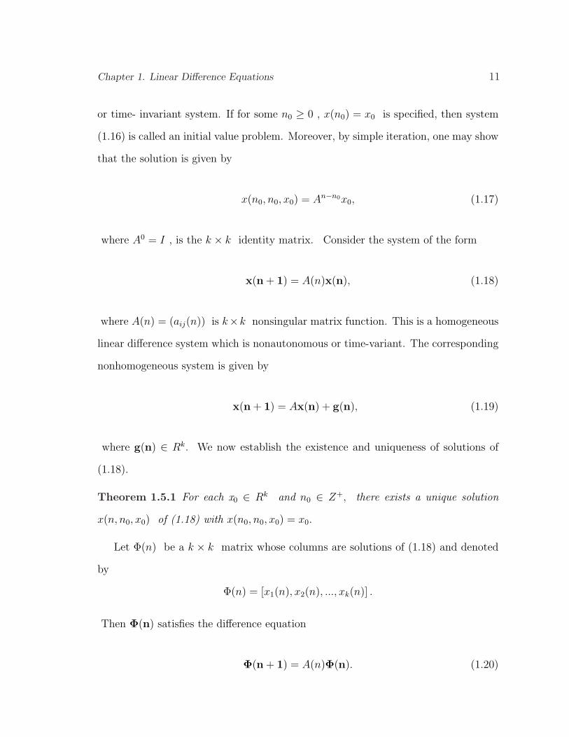
or time- invariant system. If for some n0 ≥ 0 , x(n0) = x0 is specified, then system
(1.16) is called an initial value problem. Moreover, by simple iteration, one may show
that the solution is given by
x(n0, n0, x0) = An−n0x0, (1.17)
where A0 = I , is the k × k identity matrix. Consider the system of the form
x(n + 1) = A(n)x(n), (1.18)
where A(n) = (aij(n)) is k×k nonsingular matrix function. This is a homogeneous
linear difference system which is nonautonomous or time-variant. The corresponding
nonhomogeneous system is given by
x(n + 1) = Ax(n) + g(n), (1.19)
where g(n) ∈ Rk. We now establish the existence and uniqueness of solutions of
(1.18).
Theorem 1.5.1 For each x0 ∈ Rk and n0 ∈ Z+, there exists a unique solution
x(n, n0, x0) of (1.18) with x(n0, n0, x0) = x0.
Let Φ(n) be a k × k matrix whose columns are solutions of (1.18) and denoted
by
Φ(n) = [x1(n), x2(n), ..., xk(n)] .
Then Φ(n) satisfies the difference equation
Φ(n + 1) = A(n)Φ(n). (1.20)
Chapter 1. Linear Difference Equations 12
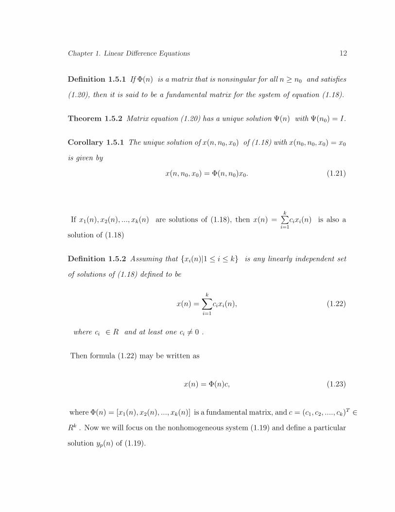
Definition 1.5.1 If Φ(n) is a matrix that is nonsingular for all n ≥ n0 and satisfies
(1.20), then it is said to be a fundamental matrix for the system of equation (1.18).
Theorem 1.5.2 Matrix equation (1.20) has a unique solution Ψ(n) with Ψ(n0) = I.
Corollary 1.5.1 The unique solution of x(n, n0, x0) of (1.18) with x(n0, n0, x0) = x0
is given by
x(n, n0, x0) = Φ(n, n0)x0. (1.21)
If x1(n), x2(n), ..., xk(n) are solutions of (1.18), then x(n) =k∑
i=1
cixi(n) is also a
solution of (1.18)
Definition 1.5.2 Assuming that xi(n)|1 ≤ i ≤ k is any linearly independent set
of solutions of (1.18) defined to be
x(n) =k∑
i=1
cixi(n), (1.22)
where ci ∈ R and at least one ci 6= 0 .
Then formula (1.22) may be written as
x(n) = Φ(n)c, (1.23)
where Φ(n) = [x1(n), x2(n), ..., xk(n)] is a fundamental matrix, and c = (c1, c2, ...., ck)T ∈
Rk . Now we will focus on the nonhomogeneous system (1.19) and define a particular
solution yp(n) of (1.19).
Chapter 1. Linear Difference Equations 13
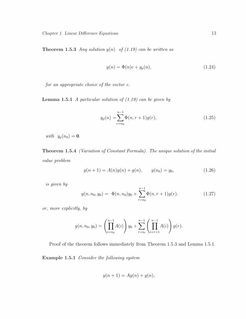
Theorem 1.5.3 Any solution y(n) of (1.19) can be written as
y(n) = Φ(n)c + yp(n), (1.24)
for an appropriate choice of the vector c.
Lemma 1.5.1 A particular solution of (1.19) can be given by
yp(n) =n−1∑r=n0
Φ(n, r + 1)g(r), (1.25)
with yp(n0) = 0.
Theorem 1.5.4 (Variation of Constant Formula). The unique solution of the initial
value problem
y(n + 1) = A(n)y(n) + g(n), y(n0) = y0, (1.26)
is given by
y(n, n0, y0) = Φ(n, n0)y0 +n−1∑r=n0
Φ(n, r + 1)g(r). (1.27)
or, more explicitly, by
y(n, n0, y0) =
(n−1∏i=n0
A(i)
)y0 +
n−1∑r=i0
(n−1∏
i=r+1
A(i)
)g(r).
Proof of the theorem follows immediately from Theorem 1.5.3 and Lemma 1.5.1.
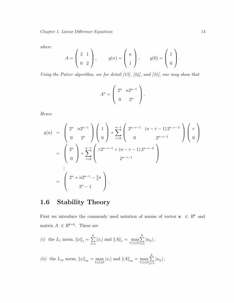
Example 1.5.1 Consider the following system
y(n + 1) = Ay(n) + g(n),
Chapter 1. Linear Difference Equations 14
where
A =
2 1
0 2
, g(n) =
n
1
, y(0) =
1
0
.
Using the Putzer algorithm, see for detail [13], [24], and [31], one may show that
An =
2n n2n−1
0 2n
.
Hence
y(n) =
2n n2n−1
0 2n
1
0
+
n−1∑r=0
2n−r−1 (n− r − 1) 2n−r−2
0 2n−r−1
r
0
=
2n
0
+
n−1∑r=0
r2n−r−1 + (n− r − 1) 2n−r−2
2n−r−1
...
=
2n + n2n−1 − 34n
2n − 1
.
1.6 Stability Theory
First we introduce the commonly used notation of norms of vector x ∈ Rk and
matrix A ∈ Rk×k. These are
(i) the L1 norm, ‖x‖1 =k∑
i=1
|xi| and ‖A‖1 = max1≤j≤k
k∑i=1
|aij| ;
(ii) the L∞ norm, ‖x‖∞ = max1≤i≤k
|xi| and ‖A‖∞ = max1≤i≤k
k∑j=1
|aij| ;
Chapter 1. Linear Difference Equations 15
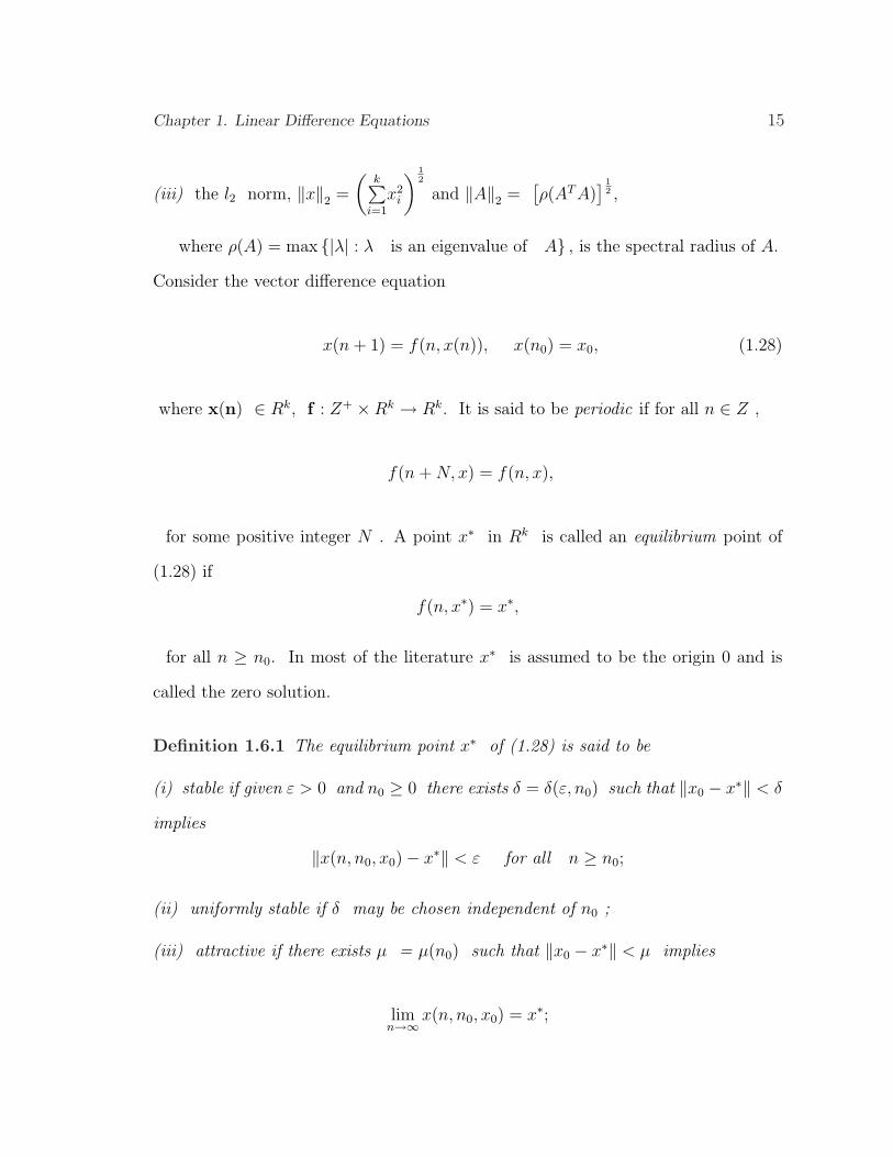
(iii) the l2 norm, ‖x‖2 =
(k∑
i=1
x2i
) 12
and ‖A‖2 =[ρ(AT A)
] 12 ,
where ρ(A) = max |λ| : λ is an eigenvalue of A , is the spectral radius of A.
Consider the vector difference equation
x(n + 1) = f(n, x(n)), x(n0) = x0, (1.28)
where x(n) ∈ Rk, f : Z+ ×Rk → Rk. It is said to be periodic if for all n ∈ Z ,
f(n + N, x) = f(n, x),
for some positive integer N . A point x∗ in Rk is called an equilibrium point of
(1.28) if
f(n, x∗) = x∗,
for all n ≥ n0. In most of the literature x∗ is assumed to be the origin 0 and is
called the zero solution.
Definition 1.6.1 The equilibrium point x∗ of (1.28) is said to be
(i) stable if given ε > 0 and n0 ≥ 0 there exists δ = δ(ε, n0) such that ‖x0 − x∗‖ < δ
implies
‖x(n, n0, x0)− x∗‖ < ε for all n ≥ n0;
(ii) uniformly stable if δ may be chosen independent of n0 ;
(iii) attractive if there exists µ = µ(n0) such that ‖x0 − x∗‖ < µ implies
limn→∞
x(n, n0, x0) = x∗;
Chapter 1. Linear Difference Equations 16
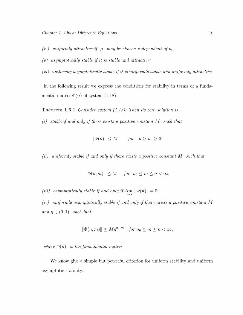
(iv) uniformly attractive if µ may be chosen independent of n0;
(v) asymptotically stable if it is stable and attractive;
(vi) uniformly asymptotically stable if it is uniformly stable and uniformly attractive.
In the following result we express the conditions for stability in terms of a funda-
mental matrix Φ(n) of system (1.18).
Theorem 1.6.1 Consider system (1.18). Then its zero solution is
(i) stable if and only if there exists a positive constant M such that
‖Φ(n)‖ ≤ M for n ≥ n0 ≥ 0;
(ii) uniformly stable if and only if there exists a positive constant M such that
‖Φ(n, m)‖ ≤ M for n0 ≤ m ≤ n < ∞;
(iii) asymptotically stable if and only if limn→∞
‖Φ(n)‖ = 0;
(iv) uniformly asymptotically stable if and only if there exists a positive constant M
and η ∈ (0, 1) such that
‖Φ(n,m)‖ ≤ Mηn−m for n0 ≤ m ≤ n < ∞,
where Φ(n) is the fundamental matrix.
We know give a simple but powerful criterion for uniform stability and uniform
asymptotic stability.
Chapter 1. Linear Difference Equations 17
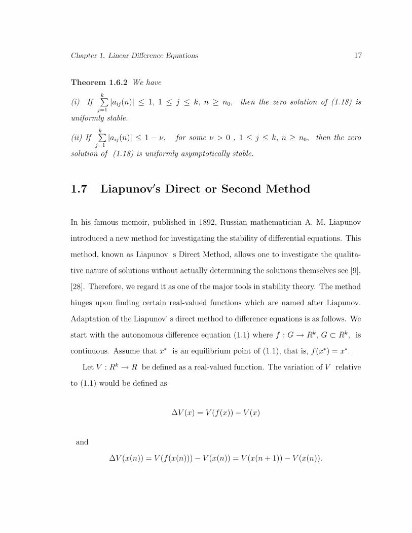
Theorem 1.6.2 We have
(i) Ifk∑
j=1
|aij(n)| ≤ 1, 1 ≤ j ≤ k, n ≥ n0, then the zero solution of (1.18) is
uniformly stable.
(ii) Ifk∑
j=1
|aij(n)| ≤ 1 − ν, for some ν > 0 , 1 ≤ j ≤ k, n ≥ n0, then the zero
solution of (1.18) is uniformly asymptotically stable.
1.7 Liapunov′s Direct or Second Method
In his famous memoir, published in 1892, Russian mathematician A. M. Liapunov
introduced a new method for investigating the stability of differential equations. This
method, known as Liapunov,s Direct Method, allows one to investigate the qualita-
tive nature of solutions without actually determining the solutions themselves see [9],
[28]. Therefore, we regard it as one of the major tools in stability theory. The method
hinges upon finding certain real-valued functions which are named after Liapunov.
Adaptation of the Liapunov,s direct method to difference equations is as follows. We
start with the autonomous difference equation (1.1) where f : G → Rk, G ⊂ Rk, is
continuous. Assume that x∗ is an equilibrium point of (1.1), that is, f(x∗) = x∗.
Let V : Rk → R be defined as a real-valued function. The variation of V relative
to (1.1) would be defined as
∆V (x) = V (f(x))− V (x)
and
∆V (x(n)) = V (f(x(n)))− V (x(n)) = V (x(n + 1))− V (x(n)).
Chapter 1. Linear Difference Equations 18
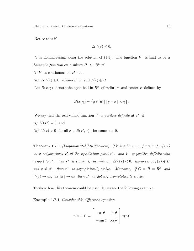
Notice that if
∆V (x) ≤ 0,
V is nonincreasing along the solution of (1.1). The function V is said to be a
Liapunov function on a subset H ⊂ Rk if
(i) V is continuous on H and
(ii) ∆V (x) ≤ 0 whenever x and f(x) ∈ H.
Let B(x, γ) denote the open ball in Rk of radius γ and center x defined by
B(x, γ) =y ∈ Rk| ‖y − x‖ < γ
.
We say that the real-valued function V is positive definite at x∗ if
(i) V (x∗) = 0 and
(ii) V (x) > 0 for all x ∈ B(x∗, γ), for some γ > 0.
Theorem 1.7.1 (Liapunov Stability Theorem). If V is a Liapunov function for (1.1)
on a neighborhood H of the equilibrium point x∗, and V is positive definite with
respect to x∗, then x∗ is stable. If, in addition, ∆V (x) < 0, whenever x, f(x) ∈ H
and x 6= x∗, then x∗ is asymptotically stable. Moreover, if G = H = Rk and
V (x) →∞, as ‖x‖ → ∞ then x∗ is globally asymptotically stable.
To show how this theorem could be used, let us see the following example.
Example 1.7.1 Consider this difference equation
x(n + 1) =
cos θ sin θ
− sin θ cos θ
x(n).
Chapter 1. Linear Difference Equations 19
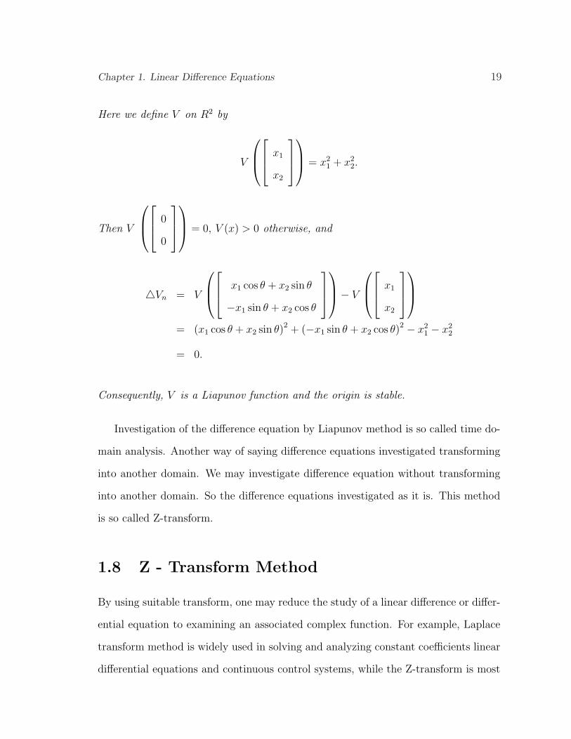
Here we define V on R2 by
V
x1
x2
= x2
1 + x22.
Then V
0
0
= 0, V (x) > 0 otherwise, and
4Vn = V
x1 cos θ + x2 sin θ
−x1 sin θ + x2 cos θ
− V
x1
x2
= (x1 cos θ + x2 sin θ)2 + (−x1 sin θ + x2 cos θ)2 − x21 − x2
2
= 0.
Consequently, V is a Liapunov function and the origin is stable.
Investigation of the difference equation by Liapunov method is so called time do-
main analysis. Another way of saying difference equations investigated transforming
into another domain. We may investigate difference equation without transforming
into another domain. So the difference equations investigated as it is. This method
is so called Z-transform.
1.8 Z - Transform Method
By using suitable transform, one may reduce the study of a linear difference or differ-
ential equation to examining an associated complex function. For example, Laplace
transform method is widely used in solving and analyzing constant coefficients linear
differential equations and continuous control systems, while the Z-transform is most
Chapter 1. Linear Difference Equations 20
suitable for linear difference equations and discrete systems. It is widely used in the
analysis and design of digital control, communication, and signal processing see [22],
[36]. The Z-transform technique is not new and may be traced back to De Moivre
around the year 1730.
The Z-transform of a sequence x(n) , which is identically zero for negative integers
n is defined
x(z) = Z(x(n)) =∞∑
j=0
x(j)z−j, (1.29)
where z is a complex number. The set of numbers z in the complex plane for which
(1.29) converges is called the region of convergence of x(z) . The most commonly
used method to find the region of convergence of (1.24) is the ratio test.
Let us discuss properties of the Z-transform.
(i) Linearity, let x(z) be the Z-transform of x(n) with radius of convergence R1
and let y(z) be the Z-transform of y(n) with radius of convergence R2. Then for
any complex numbers α, β we have
Z [αx(n) + βy(n)] = αx(z) + βy(z),
for some |z| > max(R1, R2).
(ii) Shifting , let R be the radius of convergence of x(z) . Then
(a) Right-shifting
Z [x(n− k)] = z−kx(z),
for |z| > R, where x(−i) = 0 for i = 1, 2, ..., k .
(b) Left-shifting
Z [x(n + k)] = zkx(z)−k−1∑r=0
x(r)zk−r,
Chapter 1. Linear Difference Equations 21
for |z| > R.
(iii) Convolution, a convolution ∗ of two sequences x(n), y(n) is defined by
x(n) ∗ y(n) =n∑
j=0
x(n− j) y(j) =n∑
j=0
x(j) y(n− j).
Moreover, we can obtain the sequence x(n) from x(z) using a process called the
inverse Z-transform. This process is denoted by
Z−1[x(z)
]= x(n).
Example 1.8.1 Find the Z-transform of the sequence x(n) = an .
x(z) = Z(x(n)) =∞∑
j=0
aj
zj=
∞∑j=0
(a
z
)k
=1
1− az
=z
z − a, |z| > |a| .
So far, we introduced basic theory and definitions of difference equations needed
for the coming chapters.
Chapter 2
Volterra Difference Equations
Introduction
Volterra difference equation (VDE) of the second type is of the form
x(n + 1) = Ax(n) +n∑
j=0
B(n, j)x(j), (2.1)
where A ∈ R and B : Z+ → R is a discrete function. This equation may be considered
as the discrete analogue of the famous Volterra integro-differential equations
x´(t) = Ax(t) +
t∫
0
B(t, s)x(s)ds. (2.2)
Equation (2.1) has been widely used as a mathematical model in population dy-
namics. Both equations (2.1) and (2.2) represent a system in which the future state
x(n + 1) does not depend only on the present state x(n) but also on all past states
x(n− 1), x(n− 2), ..., x(0) . Volterra difference equations (VDE) mainly arise in the
modeling process of some real phenomena or by applying a numerical method to a
Volterra integral or integro-differential equations. Actually much of their qualitative
theory remains to be developed. Stability, boundedness, and periodicity are among
the most important properties of the solution of Volterra difference equations see
22
Chapter 2. Volterra Difference Equations 23
[6]-[8], [21], [25]-[27], [29], [35], [43]. These properties will be covered in this chap-
ter. For applications of the Volterra difference equations in combinatorics see [2], in
Epidemics see [32], and in Numerical Methods for integro-differential equations see
[8].
Moreover, there is another form which is the discrete analogue of the famous
Volterra integral equations of the second type
x (t) = A +
t∫
0
B(t, s)x(s)ds, (2.3)
where A ∈ R and B : Z+ → R is a discrete function, which is
x(n) = A +n∑
j=0
B(n, j)x(j). (2.4)
We will discuss stability, asymptotic behavior, boundedness and existence of periodic
solutions of Volterra difference equations.
2.1 The Scalar Case of Volterra Difference Equa-
tions of Convolution Type
Consider the convolution type of (2.1)
x(n + 1) = Ax(n) +n∑
j=0
B(n− j)x(j), (2.5)
one of the most effective methods of dealing with (2.5) is the Z -transform method.
Chapter 2. Volterra Difference Equations 24
Let us rewrite (2.5) in the convolution form
x(n + 1) = Ax(n) + B ∗ x. (2.6)
Taking the Z-transform of both sides of (2.6), we get
zx(z)− zx(0) = Ax(z) + B(z)x(z),
which gives[z − A− B(z)
]x(z) = zx(0),
or
x(z) =zx(0)[
z − A− B(z)] . (2.7)
Let
g(z) = z − A− B(z). (2.8)
The complex function g(z) will play an important role in the stability analysis of
Volterra difference equations. It plays the role of the characteristic polynomials of
linear difference equations. In contrast to polynomials, the function g(z) may have
infinitely many zeros in the complex plane. The following lemma sheds some light on
the location of the zeros of g(z).
Lemma 2.1.1 The zeros of
g(z) = z − A− B(z),
all lie in the region |z| < c, for some real positive constant c . Moreover, g(z) has
finitely many zeros z with |z| ≥ 1 .
Chapter 2. Volterra Difference Equations 25
Proof. Suppose that all the zeros of g(z) do not lie in any region |z| < c for
any positive real number c . Then there exists a sequence zi of zeros of g(z) with
|zi| → ∞ as i →∞. Then
|zi − A| =∣∣∣B (zi)
∣∣∣ ≤∞∑
n=0
|B(n)| |zi|−n . (2.9)
Notice that the right-hand side of inequality (2.9) goes to B(0) as i → ∞, while
the left-hand side goes to ∞ as i → ∞, which is a contradiction. This proves the
first part of the lemma.
To prove the second part of the lemma, we first observe from the first part that
all zeros of g(z) with |z| ≥ 1 lie in the annulus 1 ≤ |z| ≤ c for some real number c
. We may conclude that g(z) is analytic in this annulus (1 ≤ |z| ≤ c ). Therefore,
g(z) has only finitely many zeros in the region |z| ≥ 1.
Theorem 2.1.1 The zero solution of (2.5) is uniformly asymptotically stable if and
only if
z − A− B(z) 6= 0, for all |z| ≥ 1. (2.10)
Proof. See [13].
Since locating the zeros of g(z) is impossible in most problems, to provide an
explicit conditions for the stability of (2.5), we have the following theorem.
Theorem 2.1.2 Suppose that B(n) does not change sign for n ∈ Z+. Then the zero
solution of (2.5) is asymptotically stable if
|A|+∣∣∣∣∣∞∑
n=0
B(n)
∣∣∣∣∣ < 1. (2.11)
Chapter 2. Volterra Difference Equations 26
Proof. Let β =∑∞
n=0 B(n) and D(n) = β−1B(n). Then∑∞
n=0 D(n) = 1.
Furthermore , D(1) = 1 and∣∣∣D(z)
∣∣∣ ≤ 1 for all |z| ≥ 1. Let us rewrite g(z) in the
form
g(z) = z − A− βD(z). (2.12)
To prove the asymptotic stability of zero solution of (2.5), it suffices to show that
g(z) has no zero z with |z| ≥ 1 . So assume that there exists a zero zr of g(z) with
|zr| ≥ 1. Then by (2.12) we obtain
|zr − A| =∣∣∣βD(z)
∣∣∣ ≤ |β| . (2.13)
Using condition (2.11) one concludes that
|zr| ≤ |A|+ |β| < 1,
which is a contradiction. This concludes the proof of the theorem.
Theorem 2.1.3 Suppose that B(n) does not change sign for n∈ Z+ . Then the zero
solution of (2.5) is not asymptotically stable if any one of the following conditions
hold:
i) A +∞∑
n=0
B(n) ≥ 1.
ii) A +∞∑
n=0
B(n) ≤ −1 and B(n) > 0 for some n ∈ Z+.
iii) A +∞∑
n=0
B(n) < −1 and B(n) < 0 for some n ∈ Z+,
and∞∑
n=0
B(n) is sufficiently small.
Chapter 2. Volterra Difference Equations 27
Proof. See [1], [13], [24], and [31].
The results of Theorem 2.1.2 are not extendable to uniform stability. To treat
the problem of uniform stability, the use of Liapunov functionals produce interesting
results.
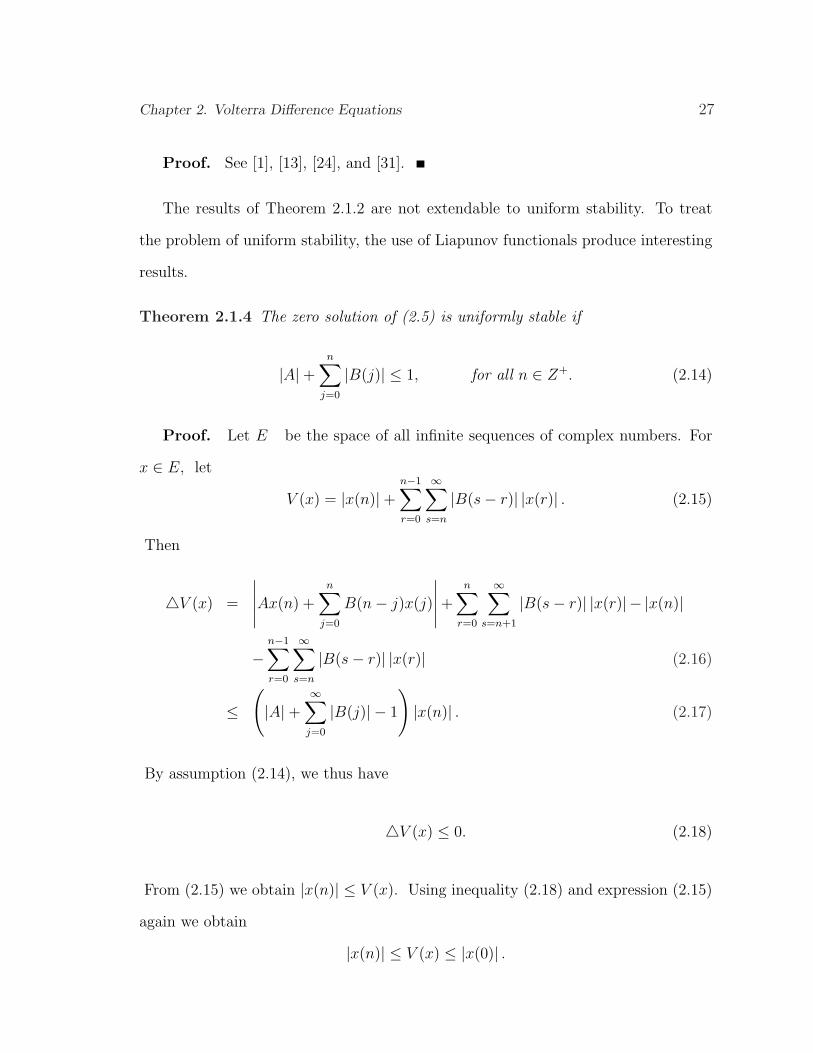
Theorem 2.1.4 The zero solution of (2.5) is uniformly stable if
|A|+n∑
j=0
|B(j)| ≤ 1, for all n ∈ Z+. (2.14)
Proof. Let E be the space of all infinite sequences of complex numbers. For
x ∈ E, let
V (x) = |x(n)|+n−1∑r=0
∞∑s=n
|B(s− r)| |x(r)| . (2.15)
Then
4V (x) =
∣∣∣∣∣Ax(n) +n∑
j=0
B(n− j)x(j)
∣∣∣∣∣ +n∑
r=0
∞∑s=n+1
|B(s− r)| |x(r)| − |x(n)|
−n−1∑r=0
∞∑s=n
|B(s− r)| |x(r)| (2.16)
≤(|A|+
∞∑j=0
|B(j)| − 1
)|x(n)| . (2.17)
By assumption (2.14), we thus have
4V (x) ≤ 0. (2.18)
From (2.15) we obtain |x(n)| ≤ V (x). Using inequality (2.18) and expression (2.15)
again we obtain
|x(n)| ≤ V (x) ≤ |x(0)| .
Chapter 2. Volterra Difference Equations 28
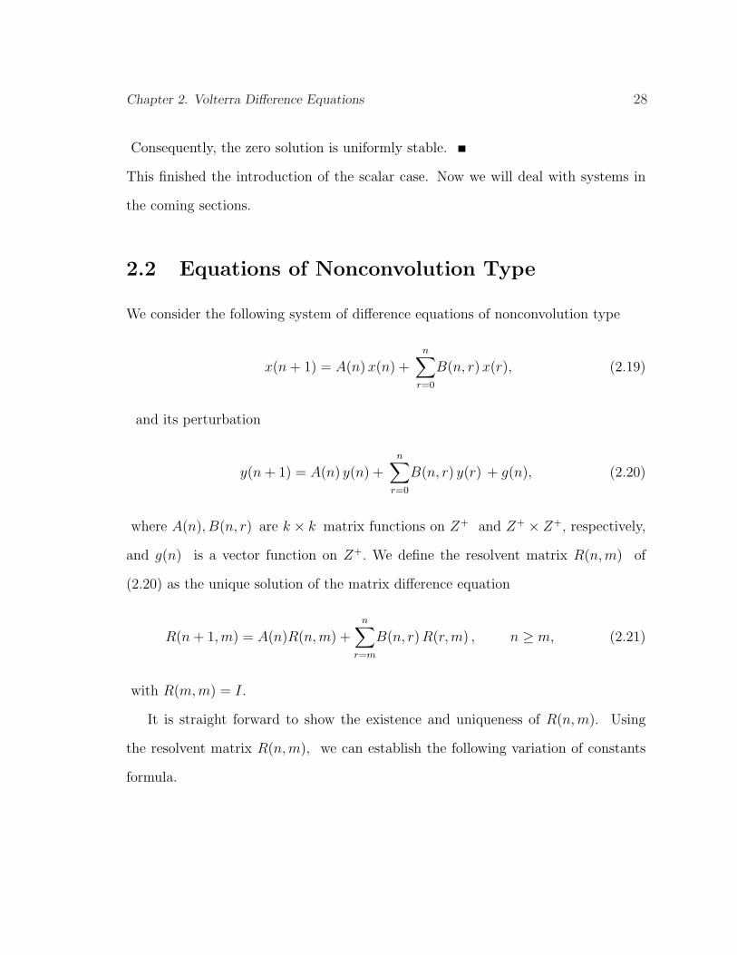
Consequently, the zero solution is uniformly stable.
This finished the introduction of the scalar case. Now we will deal with systems in
the coming sections.
2.2 Equations of Nonconvolution Type
We consider the following system of difference equations of nonconvolution type
x(n + 1) = A(n) x(n) +n∑
r=0
B(n, r) x(r), (2.19)
and its perturbation
y(n + 1) = A(n) y(n) +n∑
r=0
B(n, r) y(r) + g(n), (2.20)
where A(n), B(n, r) are k × k matrix functions on Z+ and Z+ × Z+, respectively,
and g(n) is a vector function on Z+. We define the resolvent matrix R(n,m) of
(2.20) as the unique solution of the matrix difference equation
R(n + 1,m) = A(n)R(n,m) +n∑
r=m
B(n, r) R(r,m) , n ≥ m, (2.21)
with R(m,m) = I.
It is straight forward to show the existence and uniqueness of R(n, m). Using
the resolvent matrix R(n,m), we can establish the following variation of constants
formula.
Chapter 2. Volterra Difference Equations 29
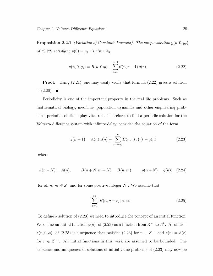
Proposition 2.2.1 (Variation of Constants Formula). The unique solution y(n, 0, y0)
of (2.20) satisfying y(0) = y0 is given by
y(n, 0, y0) = R(n, 0)y0 +n−1∑r=0
R(n, r + 1) g(r). (2.22)
Proof. Using (2.21), one may easily verify that formula (2.22) gives a solution
of (2.20).
Periodicity is one of the important property in the real life problems. Such as
mathematical biology, medicine, population dynamics and other engineering prob-
lems, periodic solutions play vital role. Therefore, to find a periodic solution for the
Volterra difference system with infinite delay, consider the equation of the form
z(n + 1) = A(n) z(n) +n∑
r=−∞B(n, r) z(r) + g(n), (2.23)
where
A(n + N) = A(n), B(n + N,m + N) = B(n,m), g(n + N) = g(n), (2.24)
for all n, m ∈ Z and for some positive integer N . We assume that
∞∑r=0
|B(n, n− r)| < ∞. (2.25)
To define a solution of (2.23) we need to introduce the concept of an initial function.
We define an initial function φ(n) of (2.23) as a function from Z− to Rk. A solution
z(n, 0, φ) of (2.23) is a sequence that satisfies (2.23) for n ∈ Z+ and z(r) = φ(r)
for r ∈ Z− . All initial functions in this work are assumed to be bounded. The
existence and uniqueness of solutions of initial value problems of (2.23) may now be
Chapter 2. Volterra Difference Equations 30
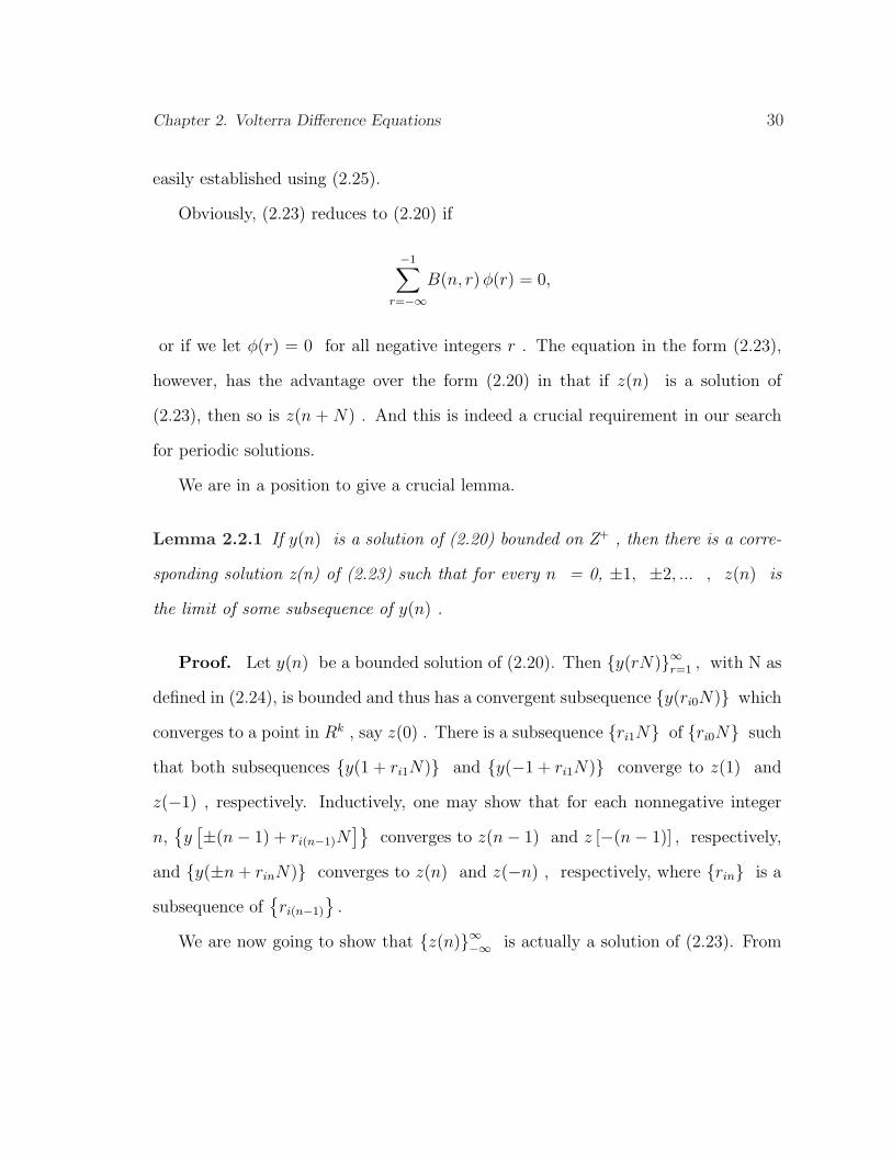
easily established using (2.25).
Obviously, (2.23) reduces to (2.20) if
−1∑r=−∞
B(n, r) φ(r) = 0,
or if we let φ(r) = 0 for all negative integers r . The equation in the form (2.23),
however, has the advantage over the form (2.20) in that if z(n) is a solution of
(2.23), then so is z(n + N) . And this is indeed a crucial requirement in our search
for periodic solutions.
We are in a position to give a crucial lemma.
Lemma 2.2.1 If y(n) is a solution of (2.20) bounded on Z+ , then there is a corre-
sponding solution z(n) of (2.23) such that for every n = 0, ±1, ±2, ... , z(n) is
the limit of some subsequence of y(n) .
Proof. Let y(n) be a bounded solution of (2.20). Then y(rN)∞r=1 , with N as
defined in (2.24), is bounded and thus has a convergent subsequence y(ri0N) which
converges to a point in Rk , say z(0) . There is a subsequence ri1N of ri0N such
that both subsequences y(1 + ri1N) and y(−1 + ri1N) converge to z(1) and
z(−1) , respectively. Inductively, one may show that for each nonnegative integer
n,y
[±(n− 1) + ri(n−1)N]
converges to z(n− 1) and z [−(n− 1)] , respectively,
and y(±n + rinN) converges to z(n) and z(−n) , respectively, where rin is a
subsequence ofri(n−1)
.
We are now going to show that z(n)∞−∞ is actually a solution of (2.23). From
Chapter 2. Volterra Difference Equations 31
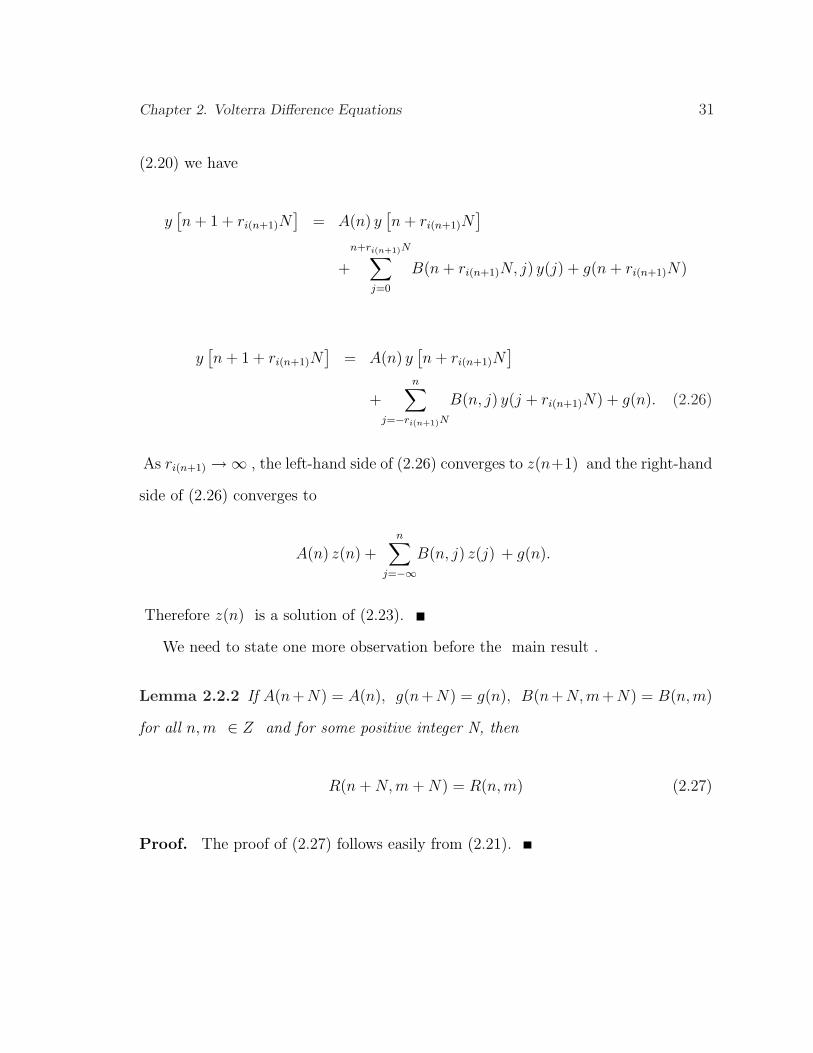
(2.20) we have
y[n + 1 + ri(n+1)N
]= A(n) y
[n + ri(n+1)N
]
+
n+ri(n+1)N∑j=0
B(n + ri(n+1)N, j) y(j) + g(n + ri(n+1)N)
y[n + 1 + ri(n+1)N
]= A(n) y
[n + ri(n+1)N
]
+n∑
j=−ri(n+1)N
B(n, j) y(j + ri(n+1)N) + g(n). (2.26)
As ri(n+1) →∞ , the left-hand side of (2.26) converges to z(n+1) and the right-hand
side of (2.26) converges to
A(n) z(n) +n∑
j=−∞B(n, j) z(j) + g(n).
Therefore z(n) is a solution of (2.23).
We need to state one more observation before the main result .
Lemma 2.2.2 If A(n+N) = A(n), g(n+N) = g(n), B(n+N, m+N) = B(n,m)
for all n,m ∈ Z and for some positive integer N, then
R(n + N,m + N) = R(n,m) (2.27)
Proof. The proof of (2.27) follows easily from (2.21).
Chapter 2. Volterra Difference Equations 32
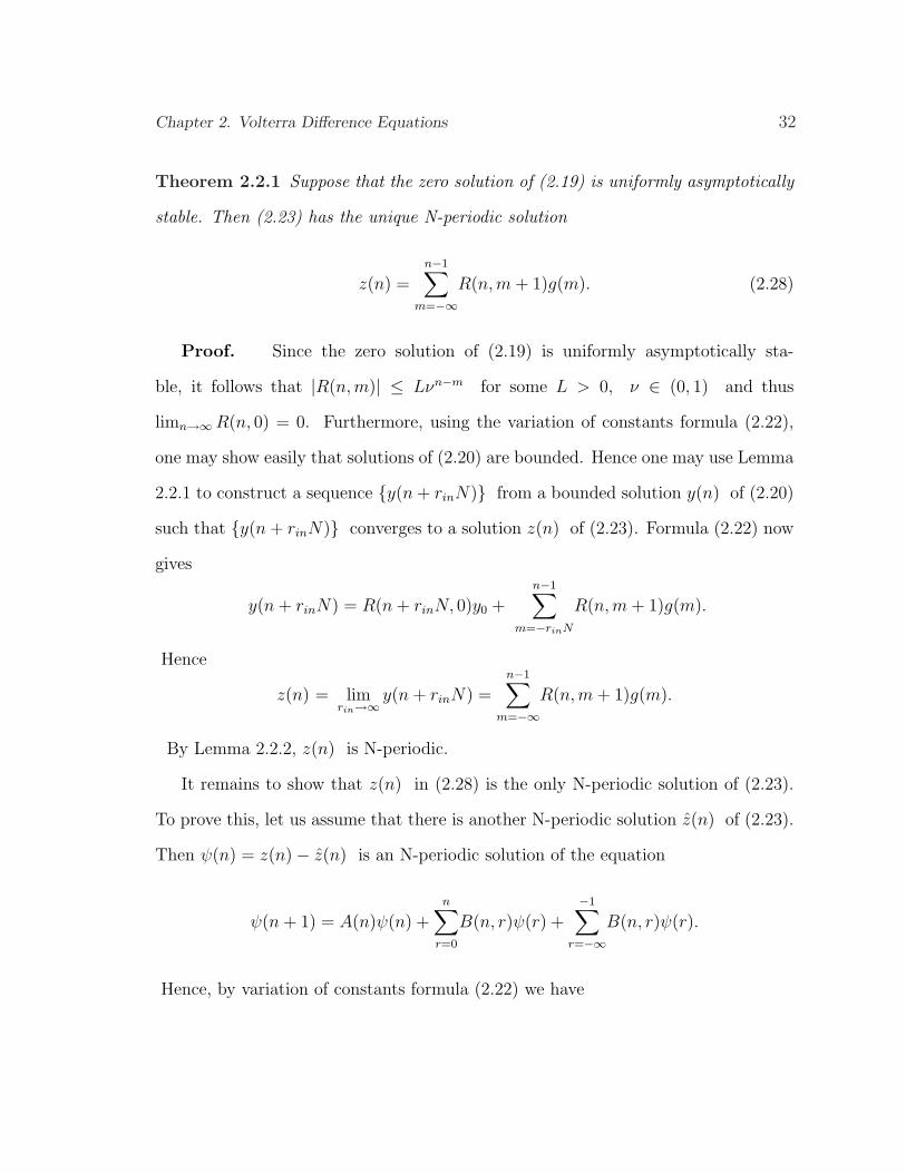
Theorem 2.2.1 Suppose that the zero solution of (2.19) is uniformly asymptotically
stable. Then (2.23) has the unique N-periodic solution
z(n) =n−1∑
m=−∞R(n, m + 1)g(m). (2.28)
Proof. Since the zero solution of (2.19) is uniformly asymptotically sta-
ble, it follows that |R(n,m)| ≤ Lνn−m for some L > 0, ν ∈ (0, 1) and thus
limn→∞ R(n, 0) = 0. Furthermore, using the variation of constants formula (2.22),
one may show easily that solutions of (2.20) are bounded. Hence one may use Lemma
2.2.1 to construct a sequence y(n + rinN) from a bounded solution y(n) of (2.20)
such that y(n + rinN) converges to a solution z(n) of (2.23). Formula (2.22) now
gives
y(n + rinN) = R(n + rinN, 0)y0 +n−1∑
m=−rinN
R(n,m + 1)g(m).
Hence
z(n) = limrin→∞
y(n + rinN) =n−1∑
m=−∞R(n,m + 1)g(m).
By Lemma 2.2.2, z(n) is N-periodic.
It remains to show that z(n) in (2.28) is the only N-periodic solution of (2.23).
To prove this, let us assume that there is another N-periodic solution z(n) of (2.23).
Then ψ(n) = z(n)− z(n) is an N-periodic solution of the equation
ψ(n + 1) = A(n)ψ(n) +n∑
r=0
B(n, r)ψ(r) +−1∑
r=−∞B(n, r)ψ(r).
Hence, by variation of constants formula (2.22) we have
Chapter 2. Volterra Difference Equations 33
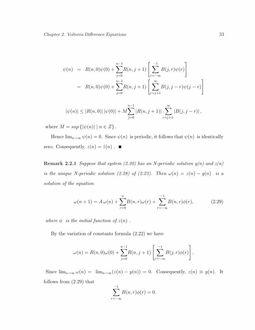
ψ(n) = R(n, 0)ψ(0) +n−1∑j=0
R(n, j + 1)
[ −1∑r=−∞
B(j, r)ψ(r)
]
= R(n, 0)ψ(0) +n−1∑j=0
R(n, j + 1)
[ ∞∑r=j+1
B(j, j − r)ψ(j − r)
]
|ψ(n)| ≤ |R(n, 0)| |ψ(0)|+ M
n−1∑j=0
|R(n, j + 1)| .
∞∑r=j+1
|B(j, j − r)| ,
where M = sup |ψ(n)| | n ∈ Z .
Hence limn→∞ ψ(n) = 0. Since ψ(n) is periodic, it follows that ψ(n) is identically
zero. Consequently, z(n) = z(n) .
Remark 2.2.1 Suppose that system (2.20) has an N-periodic solution y(n) and z(n)
is the unique N-periodic solution (2.28) of (2.23). Then ω(n) = z(n) − y(n) is a
solution of the equation
ω(n + 1) = Aω(n) +n∑
r=0
B(n, r)ω(r) +−1∑
r=−∞B(n, r)φ(r), (2.29)
where φ is the initial function of z(n) .
By the variation of constants formula (2.22) we have
ω(n) = R(n, 0)ω(0) +n−1∑j=0
R(n, j + 1)
[ −1∑r=−∞
B(j, r)φ(r)
].
Since limn→∞ ω(n) = limn→∞(z(n) − y(n)) = 0. Consequently, z(n) ≡ y(n). It
follows from (2.29) that−1∑
r=−∞B(n, r)φ(r) = 0.
Chapter 2. Volterra Difference Equations 34
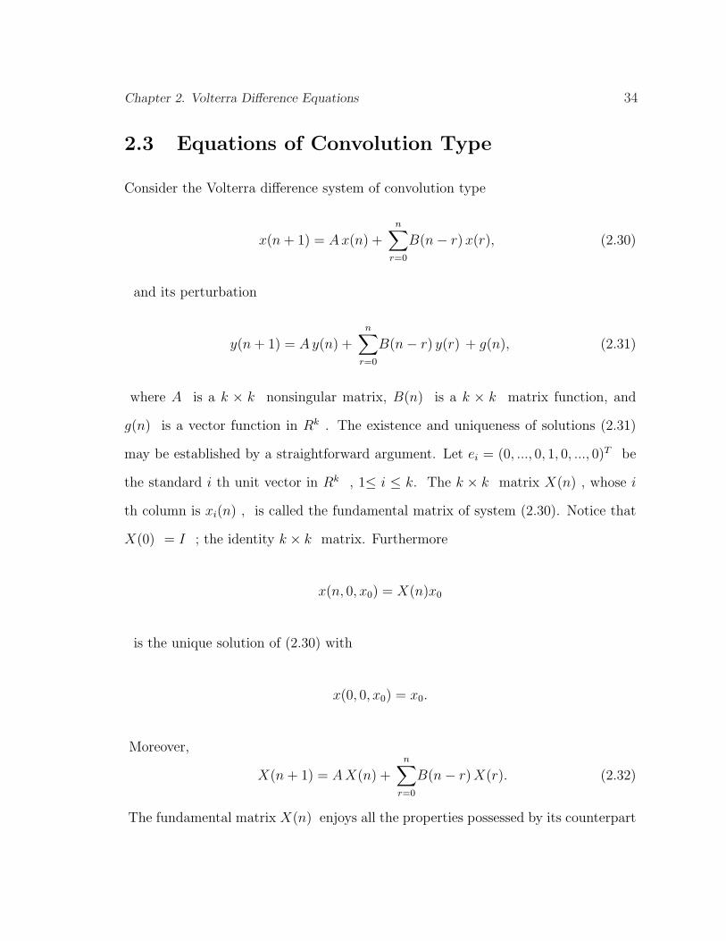
2.3 Equations of Convolution Type
Consider the Volterra difference system of convolution type
x(n + 1) = Ax(n) +n∑
r=0
B(n− r) x(r), (2.30)
and its perturbation
y(n + 1) = Ay(n) +n∑
r=0
B(n− r) y(r) + g(n), (2.31)
where A is a k × k nonsingular matrix, B(n) is a k × k matrix function, and
g(n) is a vector function in Rk . The existence and uniqueness of solutions (2.31)
may be established by a straightforward argument. Let ei = (0, ..., 0, 1, 0, ..., 0)T be
the standard i th unit vector in Rk , 1≤ i ≤ k. The k × k matrix X(n) , whose i
th column is xi(n) , is called the fundamental matrix of system (2.30). Notice that
X(0) = I ; the identity k × k matrix. Furthermore
x(n, 0, x0) = X(n)x0
is the unique solution of (2.30) with
x(0, 0, x0) = x0.
Moreover,
X(n + 1) = AX(n) +n∑
r=0
B(n− r) X(r). (2.32)
The fundamental matrix X(n) enjoys all the properties possessed by its counterpart
Chapter 2. Volterra Difference Equations 35
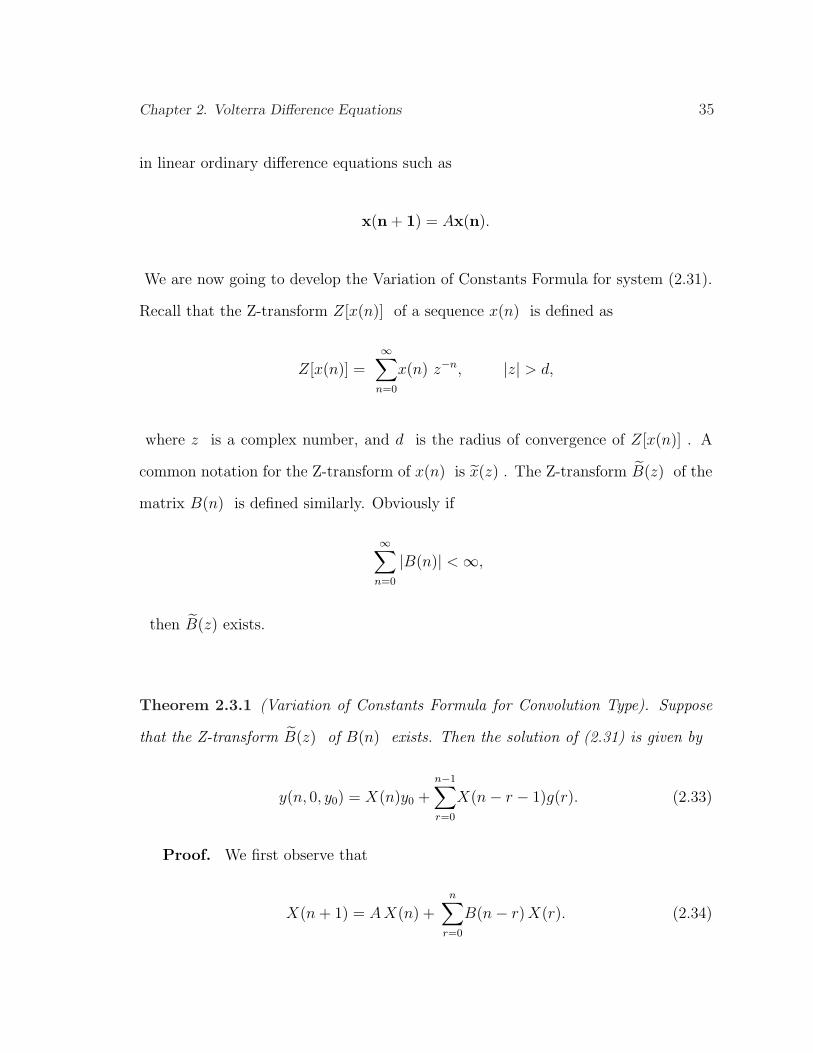
in linear ordinary difference equations such as
x(n + 1) = Ax(n).
We are now going to develop the Variation of Constants Formula for system (2.31).
Recall that the Z-transform Z[x(n)] of a sequence x(n) is defined as
Z[x(n)] =∞∑
n=0
x(n) z−n, |z| > d,
where z is a complex number, and d is the radius of convergence of Z[x(n)] . A
common notation for the Z-transform of x(n) is x(z) . The Z-transform B(z) of the
matrix B(n) is defined similarly. Obviously if
∞∑n=0
|B(n)| < ∞,
then B(z) exists.
Theorem 2.3.1 (Variation of Constants Formula for Convolution Type). Suppose
that the Z-transform B(z) of B(n) exists. Then the solution of (2.31) is given by
y(n, 0, y0) = X(n)y0 +n−1∑r=0
X(n− r − 1)g(r). (2.33)
Proof. We first observe that
X(n + 1) = AX(n) +n∑
r=0
B(n− r) X(r). (2.34)
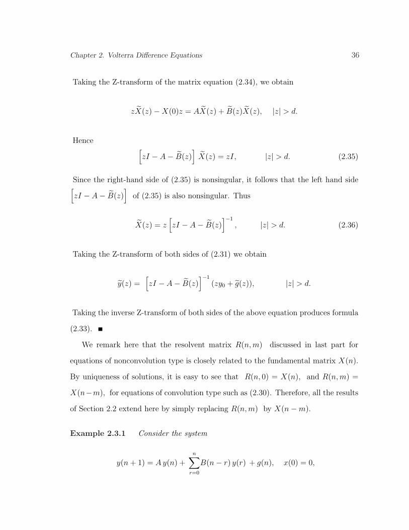
Chapter 2. Volterra Difference Equations 36
Taking the Z-transform of the matrix equation (2.34), we obtain
zX(z)−X(0)z = AX(z) + B(z)X(z), |z| > d.
Hence[zI − A− B(z)
]X(z) = zI, |z| > d. (2.35)
Since the right-hand side of (2.35) is nonsingular, it follows that the left hand side[zI − A− B(z)
]of (2.35) is also nonsingular. Thus
X(z) = z[zI − A− B(z)
]−1
, |z| > d. (2.36)
Taking the Z-transform of both sides of (2.31) we obtain
y(z) =[zI − A− B(z)
]−1
(zy0 + g(z)), |z| > d.
Taking the inverse Z-transform of both sides of the above equation produces formula
(2.33).
We remark here that the resolvent matrix R(n,m) discussed in last part for
equations of nonconvolution type is closely related to the fundamental matrix X(n).
By uniqueness of solutions, it is easy to see that R(n, 0) = X(n), and R(n,m) =
X(n−m), for equations of convolution type such as (2.30). Therefore, all the results
of Section 2.2 extend here by simply replacing R(n,m) by X(n−m).
Example 2.3.1 Consider the system
y(n + 1) = Ay(n) +n∑
r=0
B(n− r) y(r) + g(n), x(0) = 0,
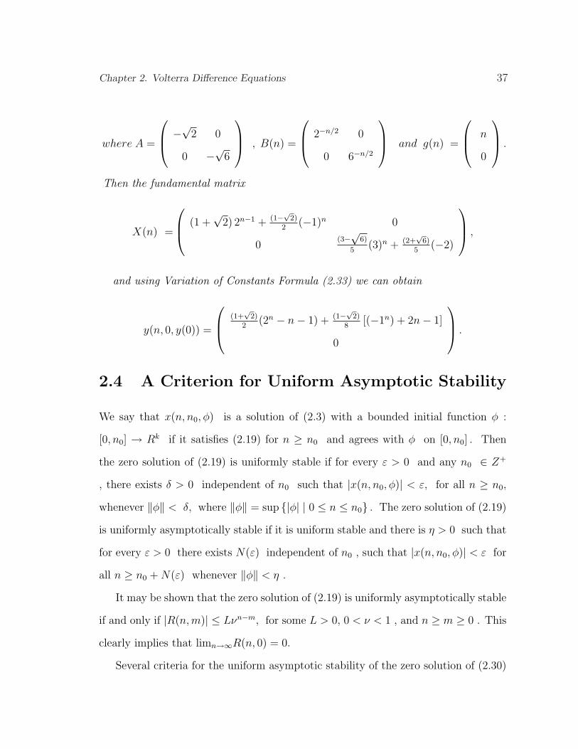
Chapter 2. Volterra Difference Equations 37
where A =
−√2 0
0 −√6
, B(n) =
2−n/2 0
0 6−n/2
and g(n) =
n
0
.
Then the fundamental matrix
X(n) =
(1 +√
2) 2n−1 + (1−√2)2
(−1)n 0
0(3−√
6)
5(3)n + (2+
√6)
5(−2)
,
and using Variation of Constants Formula (2.33) we can obtain
y(n, 0, y(0)) =
(1+√
2)2
(2n − n− 1) + (1−√2)8
[(−1n) + 2n− 1]
0
.
2.4 A Criterion for Uniform Asymptotic Stability
We say that x(n, n0, φ) is a solution of (2.3) with a bounded initial function φ :
[0, n0] → Rk if it satisfies (2.19) for n ≥ n0 and agrees with φ on [0, n0] . Then
the zero solution of (2.19) is uniformly stable if for every ε > 0 and any n0 ∈ Z+
, there exists δ > 0 independent of n0 such that |x(n, n0, φ)| < ε, for all n ≥ n0,
whenever ‖φ‖ < δ, where ‖φ‖ = sup |φ| | 0 ≤ n ≤ n0 . The zero solution of (2.19)
is uniformly asymptotically stable if it is uniform stable and there is η > 0 such that
for every ε > 0 there exists N(ε) independent of n0 , such that |x(n, n0, φ)| < ε for
all n ≥ n0 + N(ε) whenever ‖φ‖ < η .
It may be shown that the zero solution of (2.19) is uniformly asymptotically stable
if and only if |R(n,m)| ≤ Lνn−m, for some L > 0, 0 < ν < 1 , and n ≥ m ≥ 0 . This
clearly implies that limn→∞R(n, 0) = 0.
Several criteria for the uniform asymptotic stability of the zero solution of (2.30)
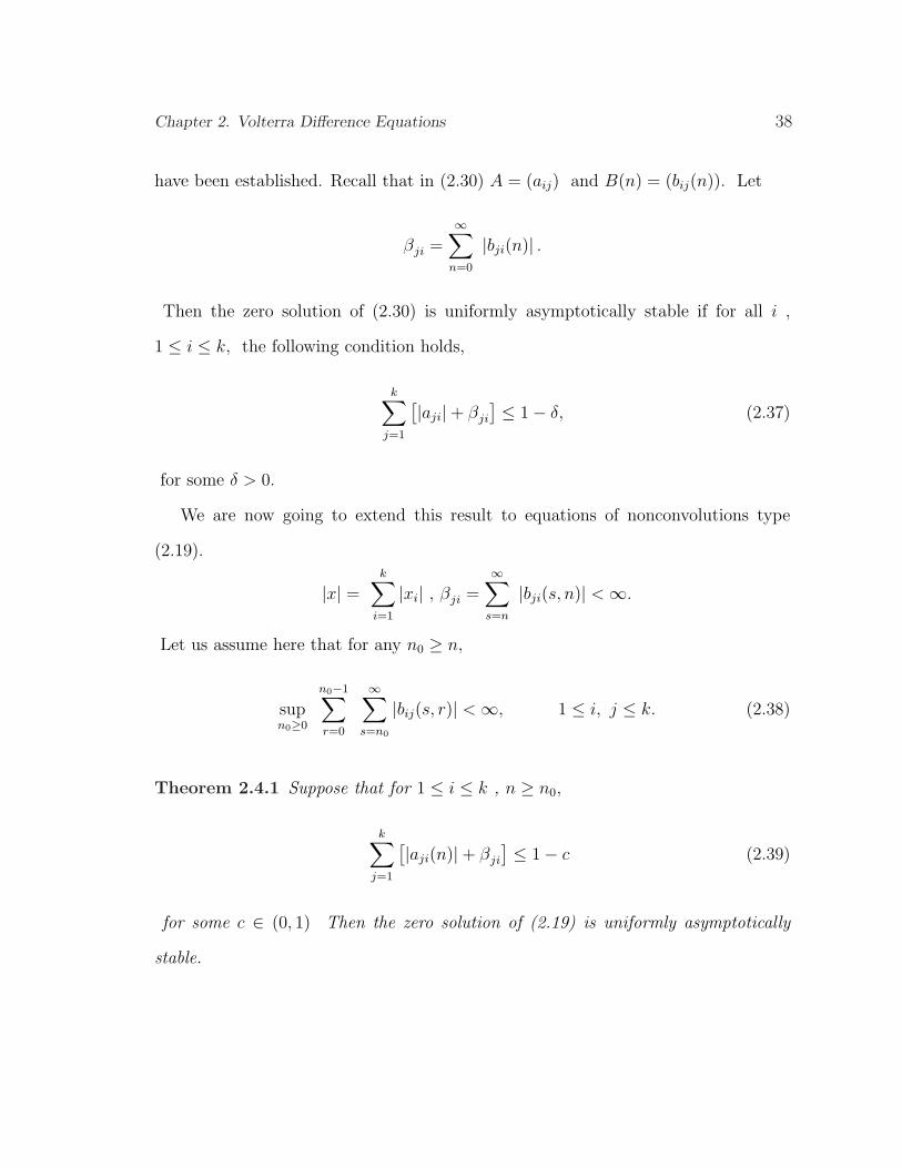
Chapter 2. Volterra Difference Equations 38
have been established. Recall that in (2.30) A = (aij) and B(n) = (bij(n)). Let
βji =∞∑
n=0
|bji(n)| .
Then the zero solution of (2.30) is uniformly asymptotically stable if for all i ,
1 ≤ i ≤ k, the following condition holds,
k∑j=1
[|aji|+ βji
] ≤ 1− δ, (2.37)
for some δ > 0.
We are now going to extend this result to equations of nonconvolutions type
(2.19).
|x| =k∑
i=1
|xi| , βji =∞∑
s=n
|bji(s, n)| < ∞.
Let us assume here that for any n0 ≥ n,
supn0≥0
n0−1∑r=0
∞∑s=n0
|bij(s, r)| < ∞, 1 ≤ i, j ≤ k. (2.38)
Theorem 2.4.1 Suppose that for 1 ≤ i ≤ k , n ≥ n0,
k∑j=1
[|aji(n)|+ βji
] ≤ 1− c (2.39)
for some c ∈ (0, 1) Then the zero solution of (2.19) is uniformly asymptotically
stable.
Chapter 2. Volterra Difference Equations 39
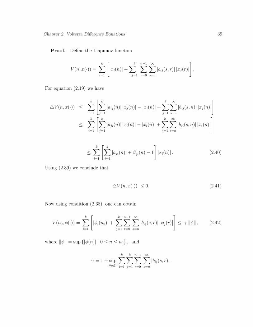
Proof. Define the Liapunov function
V (n, x(·)) =k∑
i=1
[|xi(n)|+
k∑j=1
n−1∑r=0
∞∑s=n
|bij(s, r)| |xj(r)|]
.
For equation (2.19) we have
4V (n, x(·)) ≤k∑
i=1
[k∑
j=1
|aij(n)| |xj(n)| − |xi(n)|+k∑
j=1
∞∑s=n
|bij(s, n)| |xj(n)|]
≤k∑
i=1
[k∑
j=1
|aji(n)| |xi(n)| − |xi(n)|+k∑
j=1
∞∑s=n
|bji(s, n)| |xi(n)|]
≤k∑
i=1
[k∑
j=1
|aji(n)|+ βji(n)− 1
]|xi(n)| . (2.40)
Using (2.39) we conclude that
4V (n, x(·)) ≤ 0. (2.41)
Now using condition (2.38), one can obtain
V (n0, φ(·)) =k∑
i=1
[|φi(n0)|+
k∑j=1
n−1∑r=0
∞∑s=n
|bij(s, r)|∣∣φj(r)
∣∣]≤ γ ‖φ‖ , (2.42)
where ‖φ‖ = sup |φ(n)| | 0 ≤ n ≤ n0 , and
γ = 1 + supn0≥0
k∑i=1
k∑j=1
n−1∑r=0
∞∑s=n
|bij(s, r)| .
Chapter 2. Volterra Difference Equations 40
By (2.41) and (2.42) we have
|x(n, n0, φ)| ≤ V (n, x(·)) ≤ V (n0, φ(·)) ≤ γ ‖φ‖ .
Using condition (2.39) in (2.40) yields
4V (n, x(·)) ≤ −c |x(n)| . (2.43)
This implies that the zero solution of (2.19) is uniformly asymptotically stable.
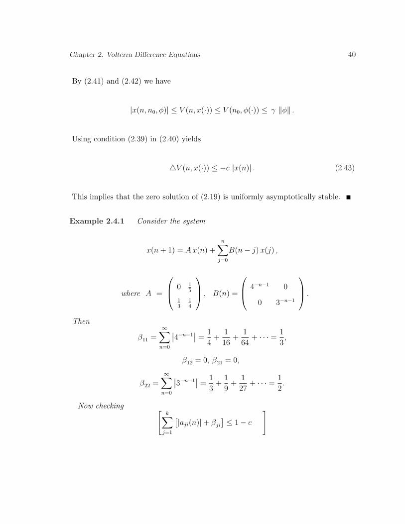
Example 2.4.1 Consider the system
x(n + 1) = Ax(n) +n∑
j=0
B(n− j) x(j) ,
where A =
0 15
13
14
, B(n) =
4−n−1 0
0 3−n−1
.
Then
β11 =∞∑
n=0
∣∣4−n−1∣∣ =
1
4+
1
16+
1
64+ · · · = 1
3,
β12 = 0, β21 = 0,
β22 =∞∑
n=0
∣∣3−n−1∣∣ =
1
3+
1
9+
1
27+ · · · = 1
2.
Now checking [k∑
j=1
[|aji(n)|+ βji
] ≤ 1− c
]
Chapter 2. Volterra Difference Equations 41
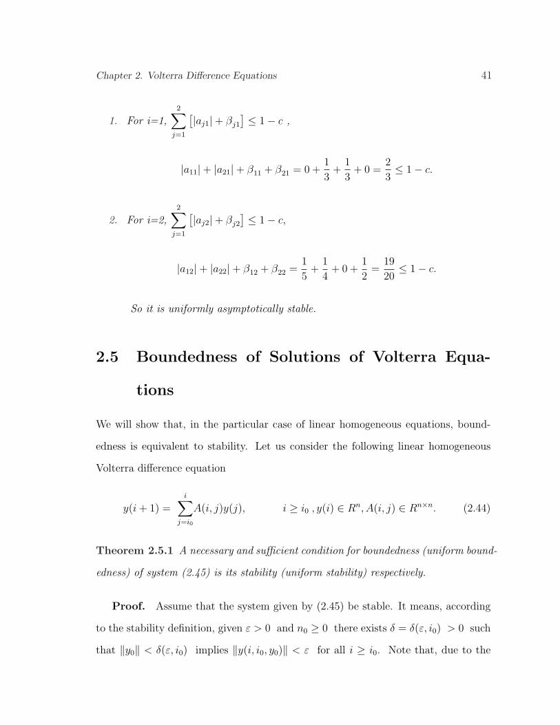
1. For i=1,2∑
j=1
[|aj1|+ βj1
] ≤ 1− c ,
|a11|+ |a21|+ β11 + β21 = 0 +1
3+
1
3+ 0 =
2
3≤ 1− c.
2. For i=2,2∑
j=1
[|aj2|+ βj2
] ≤ 1− c,
|a12|+ |a22|+ β12 + β22 =1
5+
1
4+ 0 +
1
2=
19
20≤ 1− c.
So it is uniformly asymptotically stable.
2.5 Boundedness of Solutions of Volterra Equa-
tions
We will show that, in the particular case of linear homogeneous equations, bound-
edness is equivalent to stability. Let us consider the following linear homogeneous
Volterra difference equation
y(i + 1) =i∑
j=i0
A(i, j)y(j), i ≥ i0 , y(i) ∈ Rn, A(i, j) ∈ Rn×n. (2.44)
Theorem 2.5.1 A necessary and sufficient condition for boundedness (uniform bound-
edness) of system (2.45) is its stability (uniform stability) respectively.
Proof. Assume that the system given by (2.45) be stable. It means, according
to the stability definition, given ε > 0 and n0 ≥ 0 there exists δ = δ(ε, i0) > 0 such
that ‖y0‖ < δ(ε, i0) implies ‖y(i, i0, y0)‖ < ε for all i ≥ i0. Note that, due to the
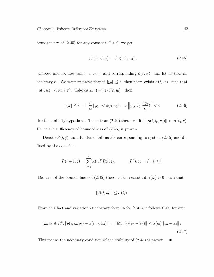
Chapter 2. Volterra Difference Equations 42
homogeneity of (2.45) for any constant C > 0 we get,
y(i, i0, Cy0) = Cy(i, i0, y0) . (2.45)
Choose and fix now some ε > 0 and corresponding δ(ε, i0) and let us take an
arbitrary r . We want to prove that if ‖y0‖ ≤ r then there exists α(i0, r) such that
‖y(i, i0)‖ < α(i0, r). Take α(i0, r) = rε/δ(ε, i0), then
‖y0‖ ≤ r =⇒ ε
α‖y0‖ < δ(α, i0) =⇒
∥∥∥y(i, i0,εy0
α)∥∥∥ < ε (2.46)
for the stability hypothesis. Then, from (2.46) there results ‖ y(i, i0, y0)‖ < α(i0, r).
Hence the sufficiency of boundedness of (2.45) is proven.
Denote R(i, j) as a fundamental matrix corresponding to system (2.45) and de-
fined by the equation
R(i + 1, j) =i∑
l=j
A(i, l)R(l, j), R(j, j) = I , i ≥ j.
Because of the boundedness of (2.45) there exists a constant α(i0) > 0 such that
‖R(i, i0)‖ ≤ α(i0).
From this fact and variation of constant formula for (2.45) it follows that, for any
y0, x0 ∈ Rn, ‖y(i, i0, y0)− x(i, i0, x0)‖ = ‖R(i, i0)(y0 − x0)‖ ≤ α(i0) ‖y0 − x0‖ .
(2.47)
This means the necessary condition of the stability of (2.45) is proven.
Chapter 2. Volterra Difference Equations 43
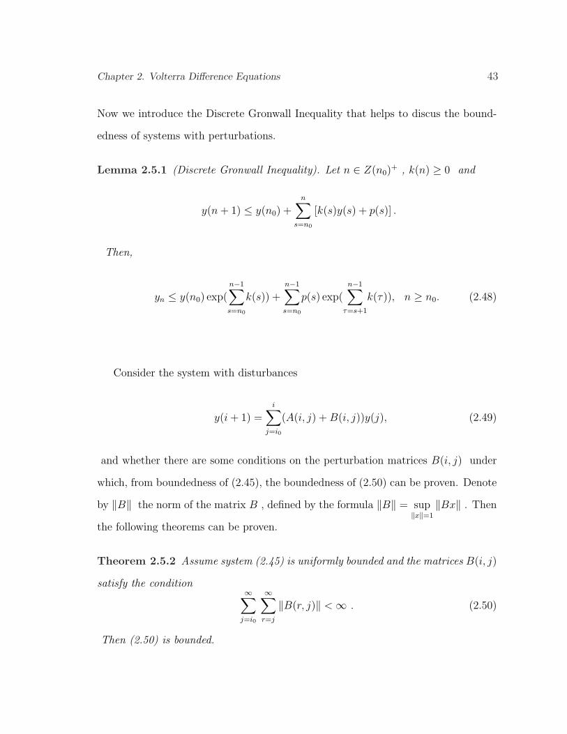
Now we introduce the Discrete Gronwall Inequality that helps to discus the bound-
edness of systems with perturbations.
Lemma 2.5.1 (Discrete Gronwall Inequality). Let n ∈ Z(n0)+ , k(n) ≥ 0 and
y(n + 1) ≤ y(n0) +n∑
s=n0
[k(s)y(s) + p(s)] .
Then,
yn ≤ y(n0) exp(n−1∑s=n0
k(s)) +n−1∑s=n0
p(s) exp(n−1∑
τ=s+1
k(τ)), n ≥ n0. (2.48)
Consider the system with disturbances
y(i + 1) =i∑
j=i0
(A(i, j) + B(i, j))y(j), (2.49)
and whether there are some conditions on the perturbation matrices B(i, j) under
which, from boundedness of (2.45), the boundedness of (2.50) can be proven. Denote
by ‖B‖ the norm of the matrix B , defined by the formula ‖B‖ = sup‖x‖=1
‖Bx‖ . Then
the following theorems can be proven.
Theorem 2.5.2 Assume system (2.45) is uniformly bounded and the matrices B(i, j)
satisfy the condition∞∑
j=i0
∞∑r=j
‖B(r, j)‖ < ∞ . (2.50)
Then (2.50) is bounded.
Chapter 2. Volterra Difference Equations 44
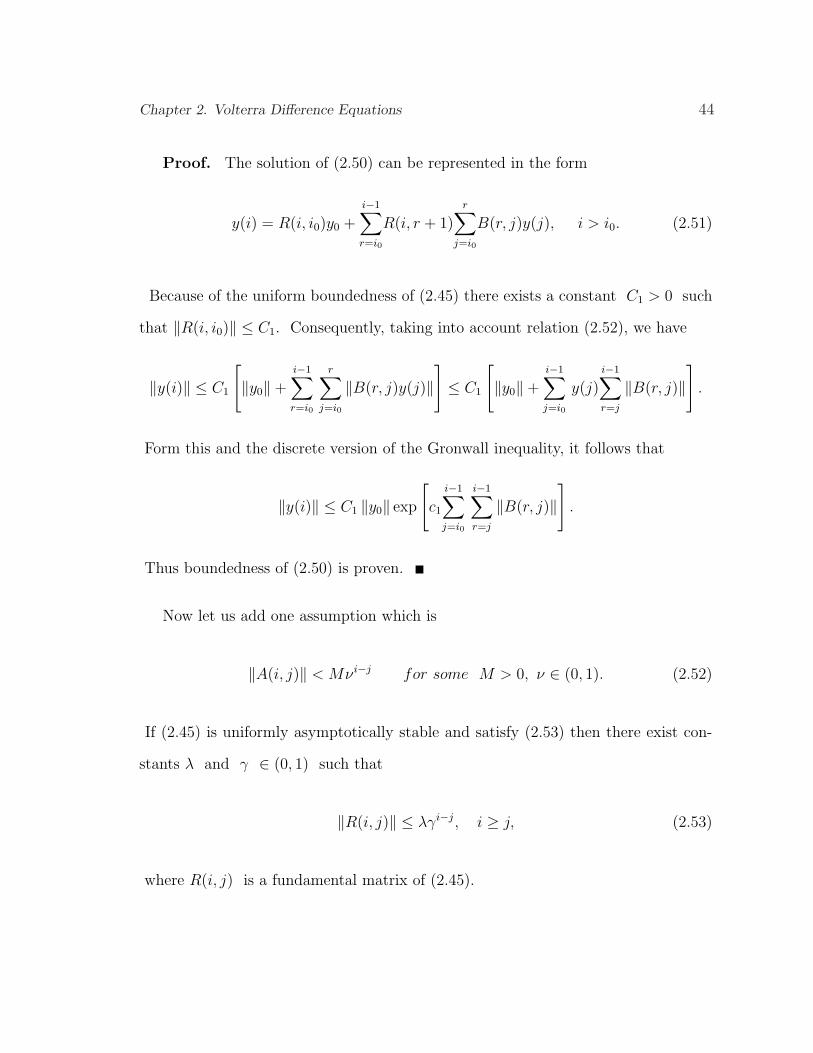
Proof. The solution of (2.50) can be represented in the form
y(i) = R(i, i0)y0 +i−1∑r=i0
R(i, r + 1)r∑
j=i0
B(r, j)y(j), i > i0. (2.51)
Because of the uniform boundedness of (2.45) there exists a constant C1 > 0 such
that ‖R(i, i0)‖ ≤ C1. Consequently, taking into account relation (2.52), we have
‖y(i)‖ ≤ C1
[‖y0‖+
i−1∑r=i0
r∑j=i0
‖B(r, j)y(j)‖]≤ C1
[‖y0‖+
i−1∑j=i0
y(j)i−1∑r=j
‖B(r, j)‖]
.
Form this and the discrete version of the Gronwall inequality, it follows that
‖y(i)‖ ≤ C1 ‖y0‖ exp
[c1
i−1∑j=i0
i−1∑r=j
‖B(r, j)‖]
.
Thus boundedness of (2.50) is proven.
Now let us add one assumption which is
‖A(i, j)‖ < Mνi−j for some M > 0, ν ∈ (0, 1). (2.52)
If (2.45) is uniformly asymptotically stable and satisfy (2.53) then there exist con-
stants λ and γ ∈ (0, 1) such that
‖R(i, j)‖ ≤ λγi−j, i ≥ j, (2.53)
where R(i, j) is a fundamental matrix of (2.45).
Chapter 2. Volterra Difference Equations 45
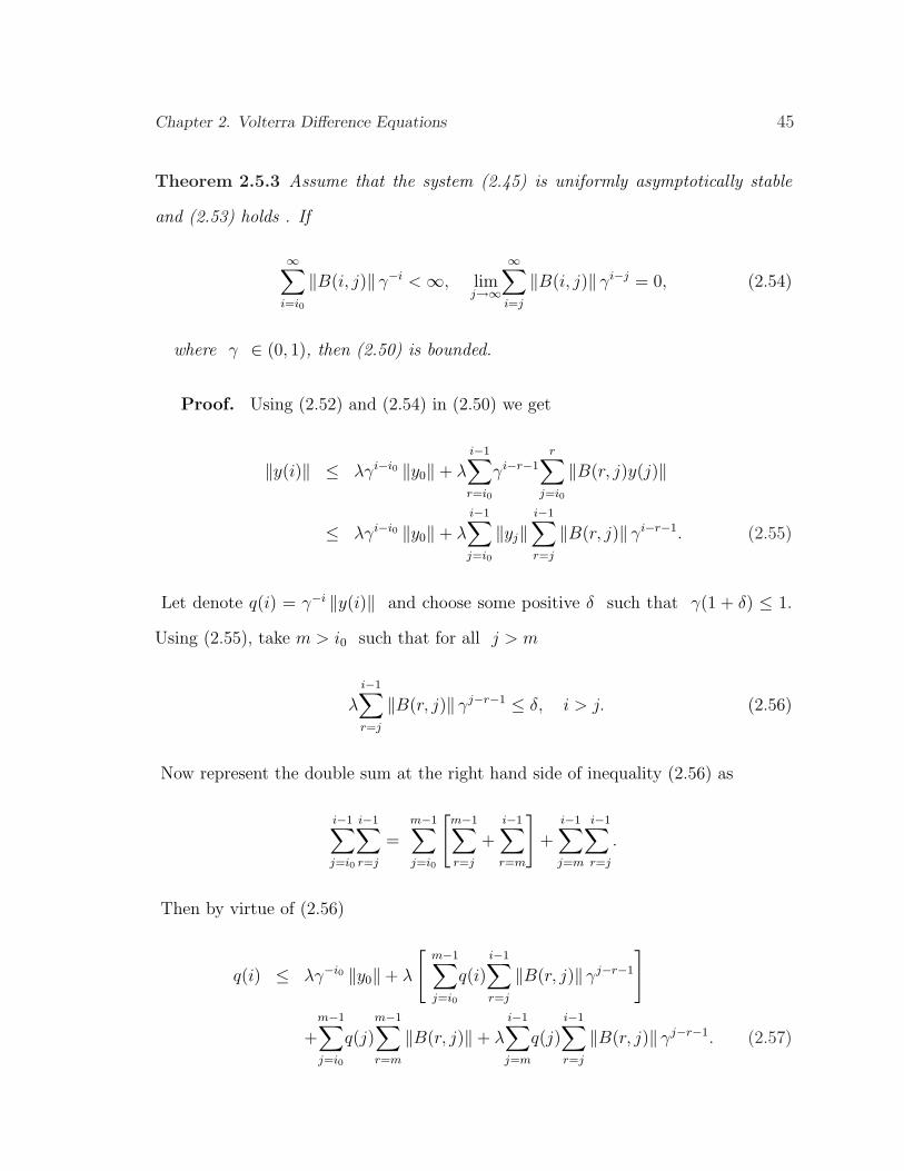
Theorem 2.5.3 Assume that the system (2.45) is uniformly asymptotically stable
and (2.53) holds . If
∞∑i=i0
‖B(i, j)‖ γ−i < ∞, limj→∞
∞∑i=j
‖B(i, j)‖ γi−j = 0, (2.54)
where γ ∈ (0, 1), then (2.50) is bounded.
Proof. Using (2.52) and (2.54) in (2.50) we get
‖y(i)‖ ≤ λγi−i0 ‖y0‖+ λ
i−1∑r=i0
γi−r−1
r∑j=i0
‖B(r, j)y(j)‖
≤ λγi−i0 ‖y0‖+ λ
i−1∑j=i0
‖yj‖i−1∑r=j
‖B(r, j)‖ γi−r−1. (2.55)
Let denote q(i) = γ−i ‖y(i)‖ and choose some positive δ such that γ(1 + δ) ≤ 1.
Using (2.55), take m > i0 such that for all j > m
λ
i−1∑r=j
‖B(r, j)‖ γj−r−1 ≤ δ, i > j. (2.56)
Now represent the double sum at the right hand side of inequality (2.56) as
i−1∑j=i0
i−1∑r=j
=m−1∑j=i0
[m−1∑r=j
+i−1∑r=m
]+
i−1∑j=m
i−1∑.
r=j
Then by virtue of (2.56)
q(i) ≤ λγ−i0 ‖y0‖+ λ
[m−1∑j=i0
q(i)i−1∑r=j
‖B(r, j)‖ γj−r−1
]
+m−1∑j=i0
q(j)m−1∑r=m
‖B(r, j)‖+ λ
i−1∑j=m
q(j)i−1∑r=j
‖B(r, j)‖ γj−r−1. (2.57)
Chapter 2. Volterra Difference Equations 46
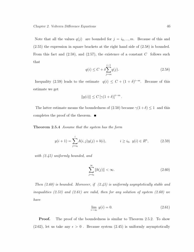
Note that all the values q(j) are bounded for j = i0, ...,m. Because of this and
(2.55) the expression in square brackets at the right hand side of (2.58) is bounded.
From this fact and (2.58), and (2.57), the existence of a constant C follows such
that
q(i) ≤ C + δ
i−1∑j=m
q(j). (2.58)
Inequality (2.59) leads to the estimate q(i) ≤ C + (1 + δ)i−m. Because of this
estimate we get
‖y(i)‖ ≤ C [γ(1 + δ)]i−m .
The latter estimate means the boundedness of (2.50) because γ(1+ δ) ≤ 1 and this
completes the proof of the theorem.
Theorem 2.5.4 Assume that the system has the form
y(i + 1) =i∑
j=i0
A(i, j)y(j) + b(i), i ≥ i0, y(i) ∈ Rn, (2.59)
with (2.45) uniformly bounded, and
∞∑j=i0
‖b(j)‖ < ∞. (2.60)
Then (2.60) is bounded. Moreover, if (2.45) is uniformly asymptotically stable and
inequalities (2.53) and (2.61) are valid, then for any solution of system (2.60) we
have
limi→∞
y(i) = 0. (2.61)
Proof. The proof of the boundedness is similar to Theorem 2.5.2. To show
(2.62), let us take any ε > 0 . Because system (2.45) is uniformly asymptotically
Chapter 2. Volterra Difference Equations 47
stable, inequality (2.54) is fulfilled. Now take and fix any N such that
λ
∞∑j=N
‖b(j)‖ < ε.
Further, similar to (2.56) using representation (2.52) we get
‖y(i)‖ ≤ λγi−i0 ‖y0‖+ λ
N∑j=i0
γi−j−1 ‖b(j)‖+ λ
∞∑j=N
‖b(j)‖ .
So, for all sufficiently large i,|y(i)| ≤ ε, for arbitrary ε > 0.
Consider equation (2.20) in the nonconvolution form, which is
y(n + 1) = A(n) y(n) +n∑
r=0
B(n, r) y(r) + g(n).
The result on the boundedness of these equations are based on growth properties of
the resolvent matrix of a linear Volterra difference equations.
First Let us introduce these assumptions:
(i) Assume that (2.54) holds for a constant γ > 1 and αF (n, u) ≤ F (n, αu), with
0 < α < 1, for all (n, x) ∈ Z+ ×R+;
(ii) Assume that (2.54) holds for a constant γ, 0 < γ < 1 and βF (n, u) ≤ F (n, βu),
β > 1 for all (n, u) ∈ Z+ ×R+;
(iii) Assume that (2.54) holds for a constant γ = 1.
Then we have the following theorem.
Theorem 2.5.5 Assume that ‖g(n, x)‖ ≤ F (n, ‖x‖), for all (n, x) ∈ Z+×Rq, where
F : Z+ × R → R+ is a monotone nondecreasing continuous function with respect
to the second variable for each fixed n ∈ Z+. Furthermore, suppose that one of the
Chapter 2. Volterra Difference Equations 48
assumptions is satisfied. Then, all solution y(n) of (2.20) such that
‖y(n0)‖ <γn0
λz(n0)
satisfies
‖y(n)‖ < γn z(n)
for all n ∈ Z+, where z(n) is a solution of the difference equation
z(n) = z(n0) +n−1∑j=n0
λ
γF (j, z(j)), z(n0) = z0.
Proof. Let us assume condition (i) holds. From the Variation of Constants
Formula for (2.20), we have
y(n) = R(n, n0)y0 +n−1∑j=n0
R(n, j + 1)g(j, y(j)), n ∈ Z+.
Thus, from the first line of the theorem, it follows that
‖y(n)‖ ≤ ‖R(n, n0)‖ ‖y(n0)‖+n−1∑j=n0
‖R(n, j + 1)‖ ‖g(j, y(j))‖
≤ λγn−n0 ‖y(n0)‖+n−1∑j=n0
λγn−j−1.F (j, ‖y(n)‖).
Hence
‖y(n)‖ γ−n ≤ λ ‖y(n0)‖ γ−n0 +n−1∑j=n0
λ.
γF (j, ‖y(n)‖ γ−j).
Chapter 2. Volterra Difference Equations 49
By the assumption λ ‖y(n0)‖ < z(n0)γn0 , we infer that
‖y(n)‖ γ−n −n−1∑j=n0
λ
γF (j, ‖y(n)‖ γ−j) < z(n)−
n−1∑j=n0
λ
γF (j, z(n)),
from which, it follows that
‖y(n)‖ < z(n)γn, n ∈ Z+,
because ‖y(n0)‖ γ−n0 < z(n0) and F (r, u) is a monotone nondecreasing continuous
function with respect to u for each r ∈ Z+.
In the case that (ii) or (iii) holds, the proof is carried out similarly, which
completes the proof of the theorem.
2.6 Volterra Difference Equations with Degener-
ate Kernels
In this section, new form will be discussed which is the implicit form of Volterra
difference equations with degenerate kernels. Stability criteria are derived. The main
tool to find the stability criteria in this analysis is the use of the new representation
formula which allows us to express the solution of Volterra difference equations with
degenerate kernels in terms of the fundamental matrix of the corresponding first-
order system of the difference equations. First, we will introduce definitions of the
degenerate kernels.
Chapter 2. Volterra Difference Equations 50
Definition 2.6.1 The kernels k is said to be degenerate or of Pincherle-Gourast type
(PG kernel) if there exist continuous q × q− matrix functions A(i, t) and B(i, s) ,
i = 1, 2, . . . , p, such that
k(t, s) =
p∑i=1
A(i, t)B(i, s). (2.62)
Consider the equation
y(n) = g(n) +n∑
j=n0
k(n, j)y(j), n ≥ n0, (2.63)
y(n) and g(n) ∈ Rq, k(n, j) ∈ Rq×q, where the kernel k(n, j) is of PG-type, i.e.,
k(n, j) =
p∑i=1
A(i, n)B(i, j), (2.64)
for some matrix sequences A(i, n) and B(i, j) ∈ Rq×q .
Consider the matrix equation
u(m,n) = I +n∑
j=m
k(n, j)u(m, j). (2.65)
Here u(m,n) is a q× q matrix which is the fundamental matrix for (2.64). Observe
that u(n+1, n) = I. This equation has a solution if, ‖k(n, j)‖ < 1. It can be checked
by direct substitution that the solution y(n) to (2.64) with n0 = 0 can be written
as
y(n) = g(n)−n∑
j=0
(u(j + 1, n)− u(j, n))g(j), n ≥ 0. (2.66)
Chapter 2. Volterra Difference Equations 51
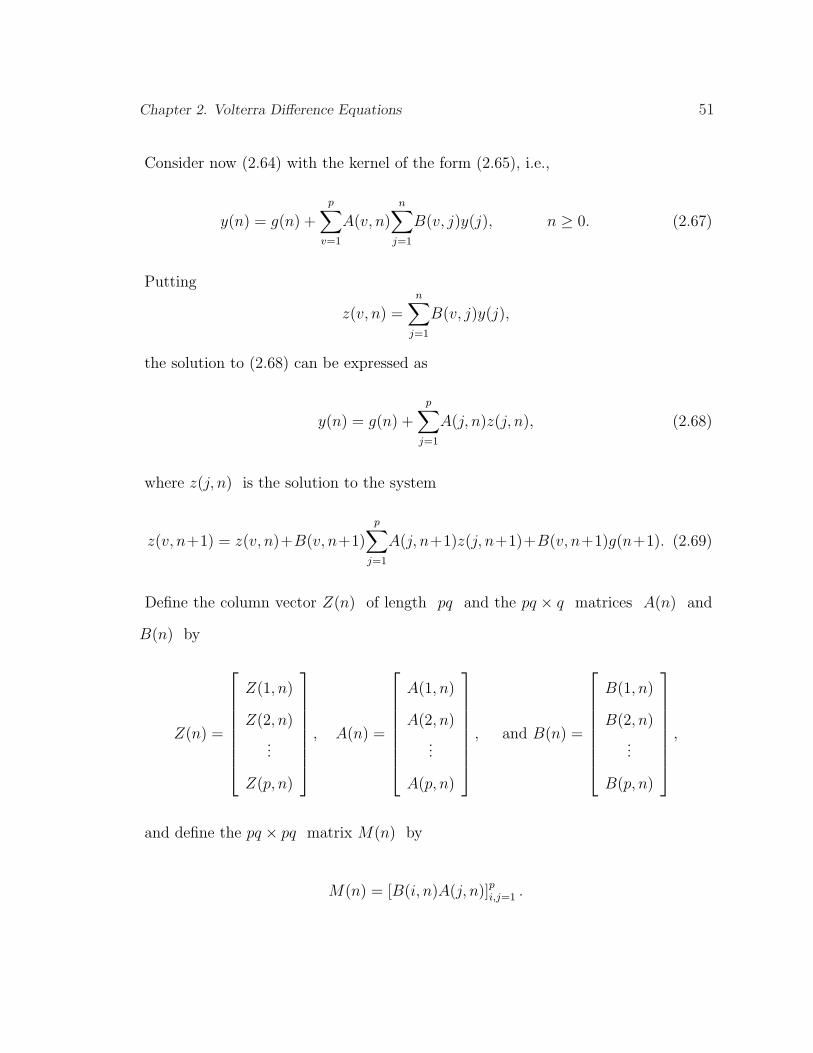
Consider now (2.64) with the kernel of the form (2.65), i.e.,
y(n) = g(n) +
p∑v=1
A(v, n)n∑
j=1
B(v, j)y(j), n ≥ 0. (2.67)
Putting
z(v, n) =n∑
j=1
B(v, j)y(j),
the solution to (2.68) can be expressed as
y(n) = g(n) +
p∑j=1
A(j, n)z(j, n), (2.68)
where z(j, n) is the solution to the system
z(v, n+1) = z(v, n)+B(v, n+1)
p∑j=1
A(j, n+1)z(j, n+1)+B(v, n+1)g(n+1). (2.69)
Define the column vector Z(n) of length pq and the pq × q matrices A(n) and
B(n) by
Z(n) =
Z(1, n)
Z(2, n)
...
Z(p, n)
, A(n) =
A(1, n)
A(2, n)
...
A(p, n)
, and B(n) =
B(1, n)
B(2, n)
...
B(p, n)
,
and define the pq × pq matrix M(n) by
M(n) = [B(i, n)A(j, n)]pi,j=1 .
Chapter 2. Volterra Difference Equations 52
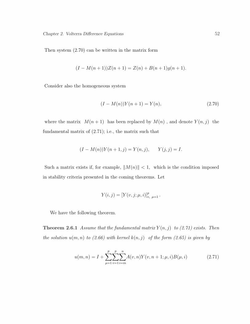
Then system (2.70) can be written in the matrix form
(I −M(n + 1))Z(n + 1) = Z(n) + B(n + 1)g(n + 1).
Consider also the homogeneous system
(I −M(n))Y (n + 1) = Y (n), (2.70)
where the matrix M(n + 1) has been replaced by M(n) , and denote Y (n, j) the
fundamental matrix of (2.71); i.e., the matrix such that
(I −M(n))Y (n + 1, j) = Y (n, j), Y (j, j) = I.
Such a matrix exists if, for example, ‖M(n)‖ < 1, which is the condition imposed
in stability criteria presented in the coming theorems. Let
Y (i, j) = [Y (v, j; µ, i)]pv, µ=1 .
We have the following theorem.
Theorem 2.6.1 Assume that the fundamental matrix Y (n, j) to (2.71) exists. Then
the solution u(m,n) to (2.66) with kernel k(n, j) of the form (2.65) is given by
u(m,n) = I +
p∑µ=1
p∑v=1
n∑i=m
A(v, n)Y (v, n + 1; µ, i)B(µ, i) (2.71)
Chapter 2. Volterra Difference Equations 53
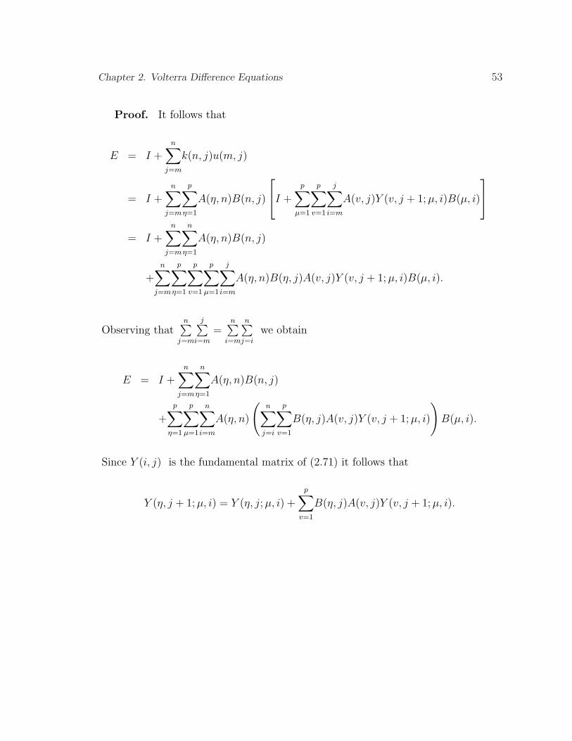
Proof. It follows that
E = I +n∑
j=m
k(n, j)u(m, j)
= I +n∑
j=m
p∑η=1
A(η, n)B(n, j)
I +
p∑µ=1
p∑v=1
j∑i=m
A(v, j)Y (v, j + 1; µ, i)B(µ, i)
= I +n∑
j=m
n∑η=1
A(η, n)B(n, j)
+n∑
j=m
p∑η=1
p∑v=1
p∑µ=1
j∑i=m
A(η, n)B(η, j)A(v, j)Y (v, j + 1; µ, i)B(µ, i).
Observing thatn∑
j=m
j∑i=m
=n∑
i=m
n∑j=i
we obtain
E = I +n∑
j=m
n∑η=1
A(η, n)B(n, j)
+
p∑η=1
p∑µ=1
n∑i=m
A(η, n)
(n∑
j=i
p∑v=1
B(η, j)A(v, j)Y (v, j + 1; µ, i)
)B(µ, i).
Since Y (i, j) is the fundamental matrix of (2.71) it follows that
Y (η, j + 1; µ, i) = Y (η, j; µ, i) +
p∑v=1
B(η, j)A(v, j)Y (v, j + 1; µ, i).
Chapter 2. Volterra Difference Equations 54
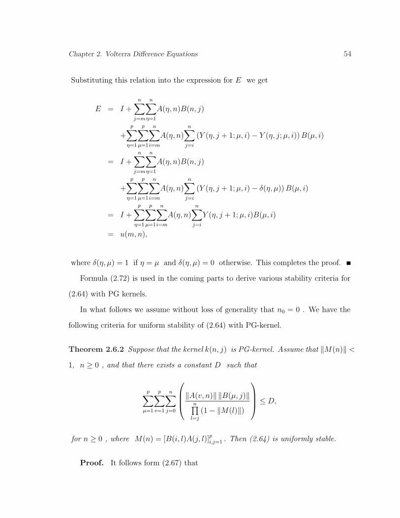
Substituting this relation into the expression for E we get
E = I +n∑
j=m
n∑η=1
A(η, n)B(n, j)
+
p∑η=1
p∑µ=1
n∑i=m
A(η, n)n∑
j=i
(Y (η, j + 1; µ, i)− Y (η, j; µ, i)) B(µ, i)
= I +n∑
j=m
n∑η=1
A(η, n)B(n, j)
+
p∑η=1
p∑µ=1
n∑i=m
A(η, n)n∑
j=i
(Y (η, j + 1; µ, i)− δ(η, µ)) B(µ, i)
= I +
p∑η=1
p∑µ=1
n∑i=m
A(η, n)n∑
j=i
Y (η, j + 1; µ, i)B(µ, i)
= u(m,n),
where δ(η, µ) = 1 if η = µ and δ(η, µ) = 0 otherwise. This completes the proof.
Formula (2.72) is used in the coming parts to derive various stability criteria for
(2.64) with PG kernels.
In what follows we assume without loss of generality that n0 = 0 . We have the
following criteria for uniform stability of (2.64) with PG-kernel.
Theorem 2.6.2 Suppose that the kernel k(n, j) is PG-kernel. Assume that ‖M(n)‖ <
1, n ≥ 0 , and that there exists a constant D such that
p∑µ=1
p∑v=1
n∑j=0
‖A(v, n)‖ ‖B(µ, j)‖
n∏l=j
(1− ‖M(l)‖)
≤ D,
for n ≥ 0 , where M(n) = [B(i, l)A(j, l)]pi,j=1 . Then (2.64) is uniformly stable.
Proof. It follows form (2.67) that
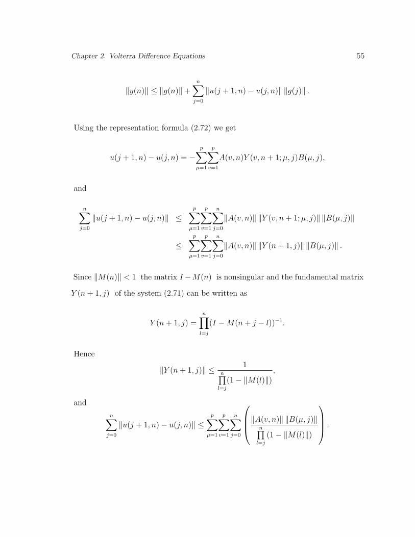
Chapter 2. Volterra Difference Equations 55
‖y(n)‖ ≤ ‖g(n)‖+n∑
j=0
‖u(j + 1, n)− u(j, n)‖ ‖g(j)‖ .
Using the representation formula (2.72) we get
u(j + 1, n)− u(j, n) = −p∑
µ=1
p∑v=1
A(v, n)Y (v, n + 1; µ, j)B(µ, j),
and
n∑j=0
‖u(j + 1, n)− u(j, n)‖ ≤p∑
µ=1
p∑v=1
n∑j=0
‖A(v, n)‖ ‖Y (v, n + 1; µ, j)‖ ‖B(µ, j)‖
≤p∑
µ=1
p∑v=1
n∑j=0
‖A(v, n)‖ ‖Y (n + 1, j)‖ ‖B(µ, j)‖ .
Since ‖M(n)‖ < 1 the matrix I−M(n) is nonsingular and the fundamental matrix
Y (n + 1, j) of the system (2.71) can be written as
Y (n + 1, j) =n∏
l=j
(I −M(n + j − l))−1.
Hence
‖Y (n + 1, j)‖ ≤ 1n∏
l=j
(1− ‖M(l)‖),
and
n∑j=0
‖u(j + 1, n)− u(j, n)‖ ≤p∑
µ=1
p∑v=1
n∑j=0
‖A(v, n)‖ ‖B(µ, j)‖
n∏l=j
(1− ‖M(l)‖)
.
Chapter 2. Volterra Difference Equations 56
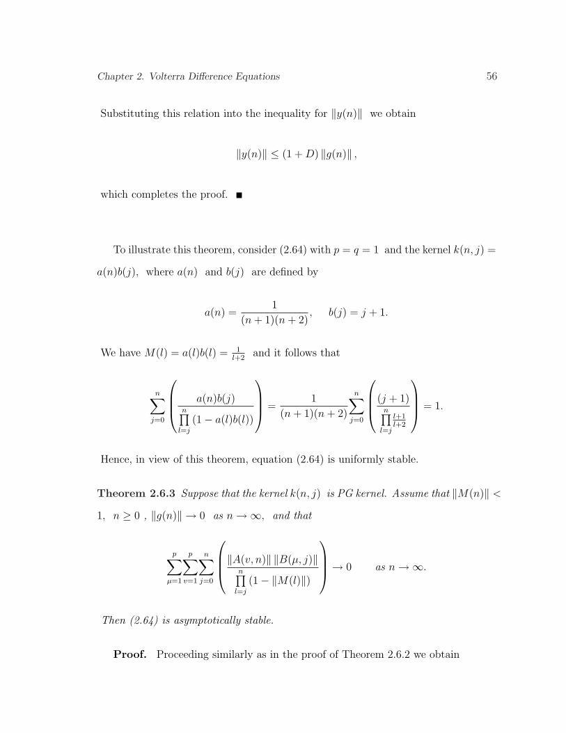
Substituting this relation into the inequality for ‖y(n)‖ we obtain
‖y(n)‖ ≤ (1 + D) ‖g(n)‖ ,
which completes the proof.
To illustrate this theorem, consider (2.64) with p = q = 1 and the kernel k(n, j) =
a(n)b(j), where a(n) and b(j) are defined by
a(n) =1
(n + 1)(n + 2), b(j) = j + 1.
We have M(l) = a(l)b(l) = 1l+2
and it follows that
n∑j=0
a(n)b(j)n∏
l=j
(1− a(l)b(l))
=
1
(n + 1)(n + 2)
n∑j=0
(j + 1)n∏
l=j
l+1l+2
= 1.
Hence, in view of this theorem, equation (2.64) is uniformly stable.
Theorem 2.6.3 Suppose that the kernel k(n, j) is PG kernel. Assume that ‖M(n)‖ <
1, n ≥ 0 , ‖g(n)‖ → 0 as n →∞, and that
p∑µ=1
p∑v=1
n∑j=0
‖A(v, n)‖ ‖B(µ, j)‖
n∏l=j
(1− ‖M(l)‖)
→ 0 as n →∞.
Then (2.64) is asymptotically stable.
Proof. Proceeding similarly as in the proof of Theorem 2.6.2 we obtain
Chapter 2. Volterra Difference Equations 57
p∑µ=1
p∑v=1
n∑j=0
‖A(v, n)‖ ‖B(µ, j)‖
n∏l=j
(1− ‖M(l)‖)
→ 0 as n →∞,
and completes the proof of the theorem.
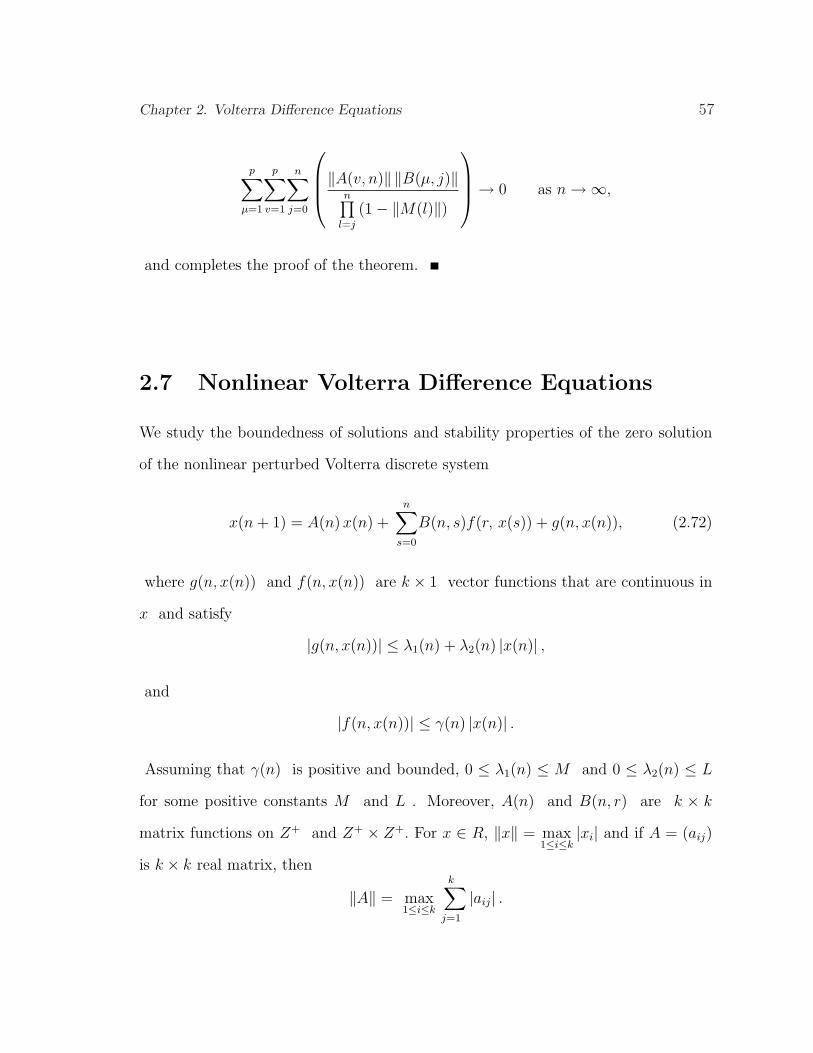
2.7 Nonlinear Volterra Difference Equations
We study the boundedness of solutions and stability properties of the zero solution
of the nonlinear perturbed Volterra discrete system
x(n + 1) = A(n) x(n) +n∑
s=0
B(n, s)f(r, x(s)) + g(n, x(n)), (2.72)
where g(n, x(n)) and f(n, x(n)) are k × 1 vector functions that are continuous in
x and satisfy
|g(n, x(n))| ≤ λ1(n) + λ2(n) |x(n)| ,
and
|f(n, x(n))| ≤ γ(n) |x(n)| .
Assuming that γ(n) is positive and bounded, 0 ≤ λ1(n) ≤ M and 0 ≤ λ2(n) ≤ L
for some positive constants M and L . Moreover, A(n) and B(n, r) are k × k
matrix functions on Z+ and Z+ × Z+. For x ∈ R, ‖x‖ = max1≤i≤k
|xi| and if A = (aij)
is k × k real matrix, then
‖A‖ = max1≤i≤k
k∑j=1
|aij| .
Chapter 2. Volterra Difference Equations 58
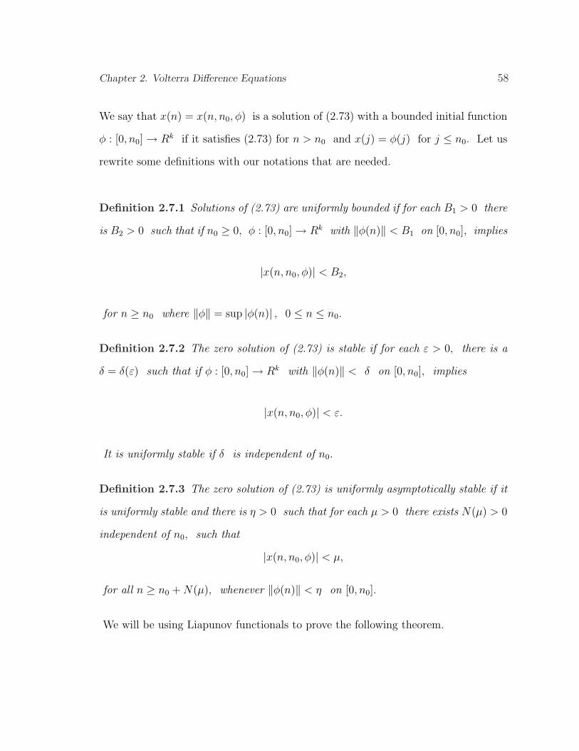
We say that x(n) = x(n, n0, φ) is a solution of (2.73) with a bounded initial function
φ : [0, n0] → Rk if it satisfies (2.73) for n > n0 and x(j) = φ(j) for j ≤ n0. Let us
rewrite some definitions with our notations that are needed.
Definition 2.7.1 Solutions of (2.73) are uniformly bounded if for each B1 > 0 there
is B2 > 0 such that if n0 ≥ 0, φ : [0, n0] → Rk with ‖φ(n)‖ < B1 on [0, n0], implies
|x(n, n0, φ)| < B2,
for n ≥ n0 where ‖φ‖ = sup |φ(n)| , 0 ≤ n ≤ n0.
Definition 2.7.2 The zero solution of (2.73) is stable if for each ε > 0, there is a
δ = δ(ε) such that if φ : [0, n0] → Rk with ‖φ(n)‖ < δ on [0, n0], implies
|x(n, n0, φ)| < ε.
It is uniformly stable if δ is independent of n0.
Definition 2.7.3 The zero solution of (2.73) is uniformly asymptotically stable if it
is uniformly stable and there is η > 0 such that for each µ > 0 there exists N(µ) > 0
independent of n0, such that
|x(n, n0, φ)| < µ,
for all n ≥ n0 + N(µ), whenever ‖φ(n)‖ < η on [0, n0].
We will be using Liapunov functionals to prove the following theorem.
Chapter 2. Volterra Difference Equations 59
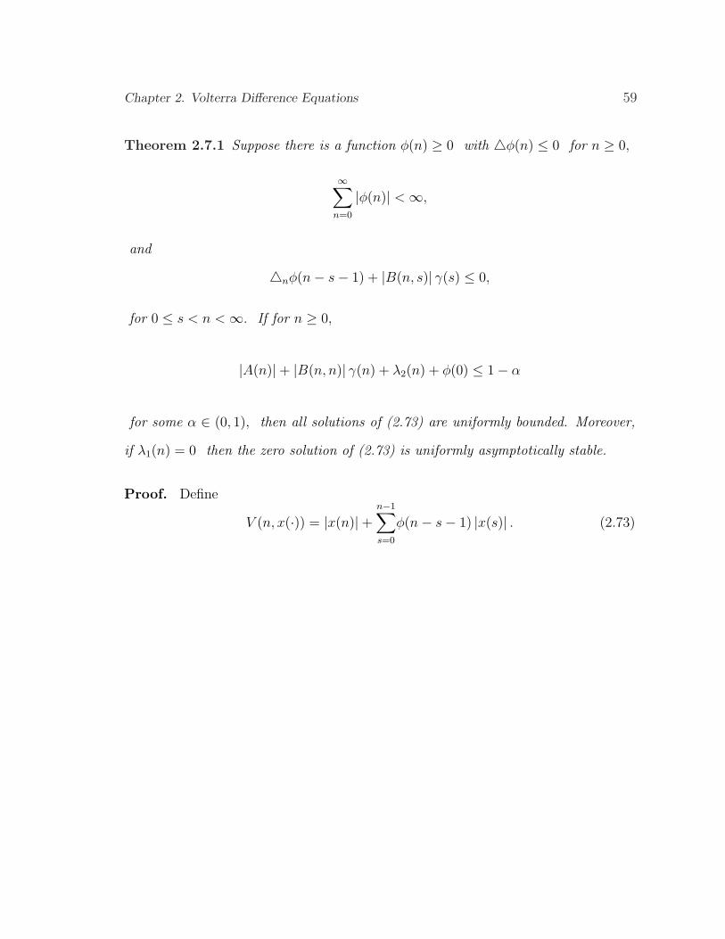
Theorem 2.7.1 Suppose there is a function φ(n) ≥ 0 with 4φ(n) ≤ 0 for n ≥ 0,
∞∑n=0
|φ(n)| < ∞,
and
4nφ(n− s− 1) + |B(n, s)| γ(s) ≤ 0,
for 0 ≤ s < n < ∞. If for n ≥ 0,
|A(n)|+ |B(n, n)| γ(n) + λ2(n) + φ(0) ≤ 1− α
for some α ∈ (0, 1), then all solutions of (2.73) are uniformly bounded. Moreover,
if λ1(n) = 0 then the zero solution of (2.73) is uniformly asymptotically stable.
Proof. Define
V (n, x(·)) = |x(n)|+n−1∑s=0
φ(n− s− 1) |x(s)| . (2.73)
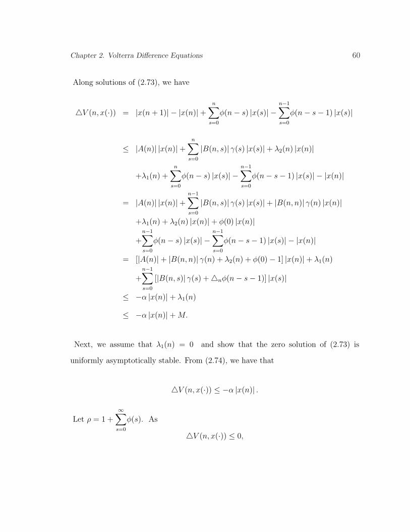
Chapter 2. Volterra Difference Equations 60
Along solutions of (2.73), we have
4V (n, x(·)) = |x(n + 1)| − |x(n)|+n∑
s=0
φ(n− s) |x(s)| −n−1∑s=0
φ(n− s− 1) |x(s)|
≤ |A(n)| |x(n)|+n∑
s=0
|B(n, s)| γ(s) |x(s)|+ λ2(n) |x(n)|
+λ1(n) +n∑
s=0
φ(n− s) |x(s)| −n−1∑s=0
φ(n− s− 1) |x(s)| − |x(n)|
= |A(n)| |x(n)|+n−1∑s=0
|B(n, s)| γ(s) |x(s)|+ |B(n, n)| γ(n) |x(n)|
+λ1(n) + λ2(n) |x(n)|+ φ(0) |x(n)|
+n−1∑s=0
φ(n− s) |x(s)| −n−1∑s=0
φ(n− s− 1) |x(s)| − |x(n)|
= [|A(n)|+ |B(n, n)| γ(n) + λ2(n) + φ(0)− 1] |x(n)|+ λ1(n)
+n−1∑s=0
[|B(n, s)| γ(s) +4nφ(n− s− 1)] |x(s)|
≤ −α |x(n)|+ λ1(n)
≤ −α |x(n)|+ M.
Next, we assume that λ1(n) = 0 and show that the zero solution of (2.73) is
uniformly asymptotically stable. From (2.74), we have that
4V (n, x(·)) ≤ −α |x(n)| .
Let ρ = 1 +∞∑
s=0
φ(s). As
4V (n, x(·)) ≤ 0,
Chapter 2. Volterra Difference Equations 61
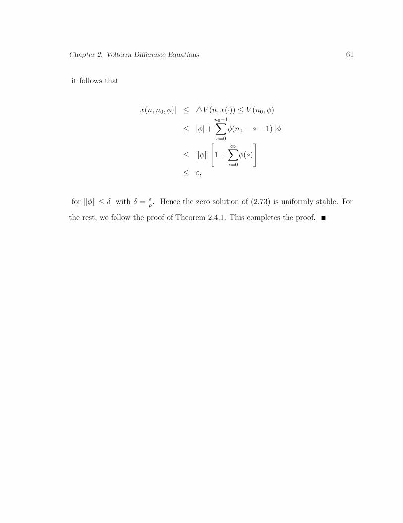
it follows that
|x(n, n0, φ)| ≤ 4V (n, x(·)) ≤ V (n0, φ)
≤ |φ|+n0−1∑s=0
φ(n0 − s− 1) |φ|
≤ ‖φ‖[1 +
∞∑s=0
φ(s)
]
≤ ε,
for ‖φ‖ ≤ δ with δ = ερ. Hence the zero solution of (2.73) is uniformly stable. For
the rest, we follow the proof of Theorem 2.4.1. This completes the proof.
Chapter 3
Discretization of Volterra
Equations
In this chapter we will establish the discrete form of the Volterra integral equa-
tions and the Volterra integro-differential equations by the generation of quadrature
weights of Backward Euler, Trapezoidal, and Simpson & Trapezoidal method and
the Linear Multistep methods. For existence, uniqueness, and stability properties of
these methods see [3], [5], [11], [20], [37], [39], [40].
3.1 Discretization of Volterra Integral and Integro-
differential Equations
Let us consider the scalar linear Volterra integral equation
y(t) = g(t) +
t∫
t0
k(t, s) y(s)ds, t ∈ [t0, T ], y, g, k ∈ R. (3.1)
The application of a Direct Quadrature method to (3.1) leads to
yn = gn + h
n∑
l=0
wn,l kn,l yl, n ≥ n0, (3.2)
62
Chapter 3. Discretization of Volterra Equations 63
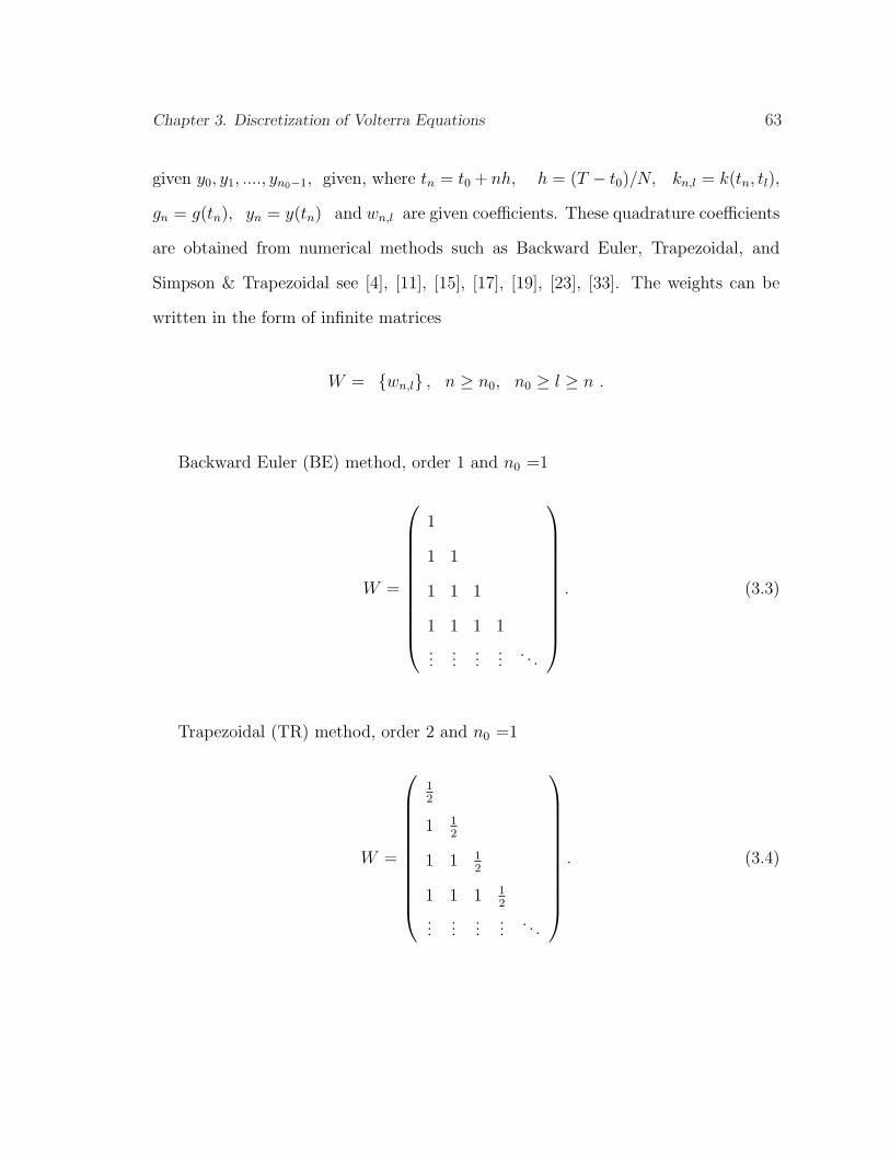
given y0, y1, ...., yn0−1, given, where tn = t0 + nh, h = (T − t0)/N, kn,l = k(tn, tl),
gn = g(tn), yn = y(tn) and wn,l are given coefficients. These quadrature coefficients
are obtained from numerical methods such as Backward Euler, Trapezoidal, and
Simpson & Trapezoidal see [4], [11], [15], [17], [19], [23], [33]. The weights can be
written in the form of infinite matrices
W = wn,l , n ≥ n0, n0 ≥ l ≥ n .
Backward Euler (BE) method, order 1 and n0 =1
W =
1
1 1
1 1 1
1 1 1 1
......
......
. . .
. (3.3)
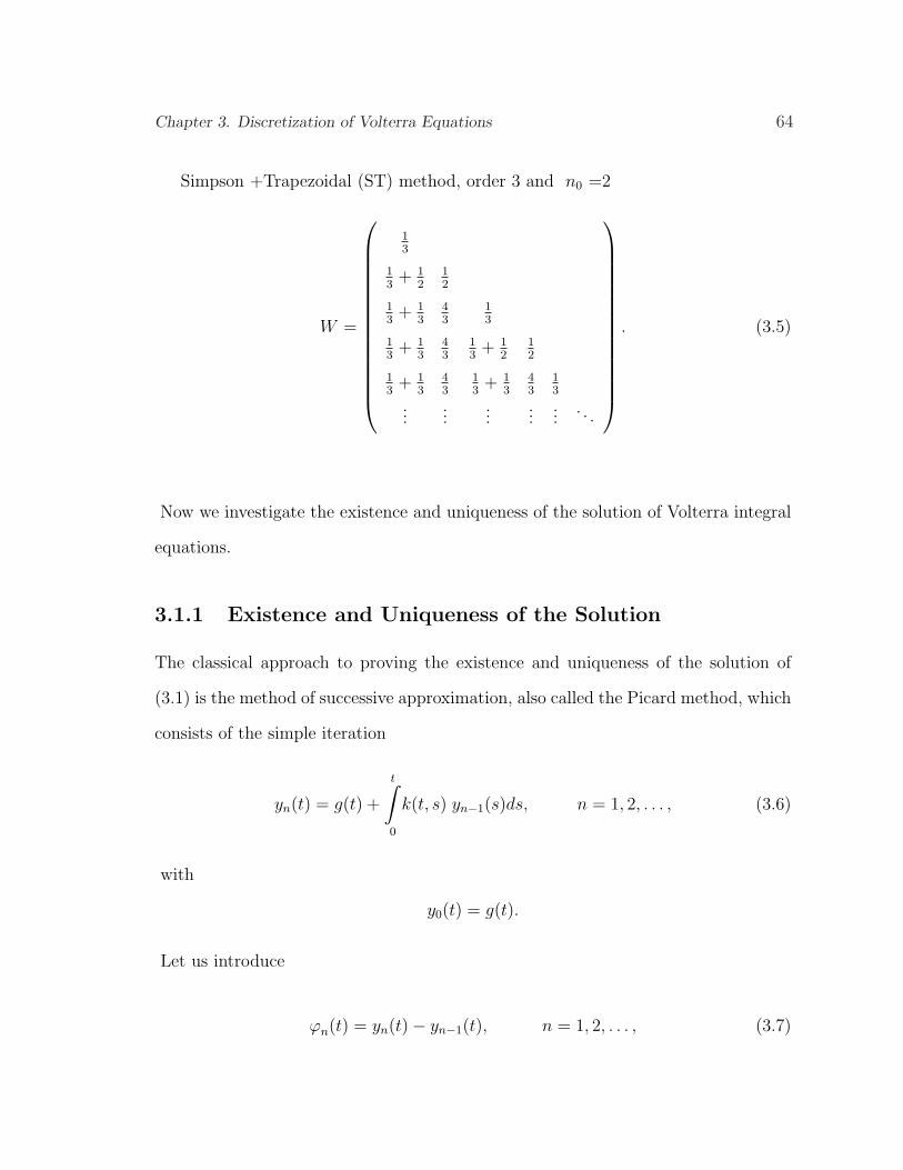
Trapezoidal (TR) method, order 2 and n0 =1
W =
12
1 12
1 1 12
1 1 1 12
......
......
. . .
. (3.4)
Chapter 3. Discretization of Volterra Equations 64
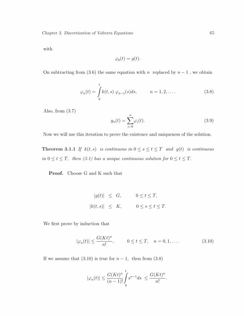
Simpson +Trapezoidal (ST) method, order 3 and n0 =2
W =
13
13
+ 12
12
13
+ 13
43
13
13
+ 13
43
13
+ 12
12
13
+ 13
43
13
+ 13
43
13
......
......
.... . .
. (3.5)
Now we investigate the existence and uniqueness of the solution of Volterra integral
equations.
3.1.1 Existence and Uniqueness of the Solution
The classical approach to proving the existence and uniqueness of the solution of
(3.1) is the method of successive approximation, also called the Picard method, which
consists of the simple iteration
yn(t) = g(t) +
t∫
0
k(t, s) yn−1(s)ds, n = 1, 2, . . . , (3.6)
with
y0(t) = g(t).
Let us introduce
ϕn(t) = yn(t)− yn−1(t), n = 1, 2, . . . , (3.7)
Chapter 3. Discretization of Volterra Equations 65
with
ϕ0(t) = g(t).
On subtracting from (3.6) the same equation with n replaced by n− 1 , we obtain
ϕn(t) =
t∫
0
k(t, s) ϕn−1(s)ds, n = 1, 2, . . . . (3.8)
Also, from (3.7)
yn(t) =n∑
i=0
ϕi(t). (3.9)
Now we will use this iteration to prove the existence and uniqueness of the solution.
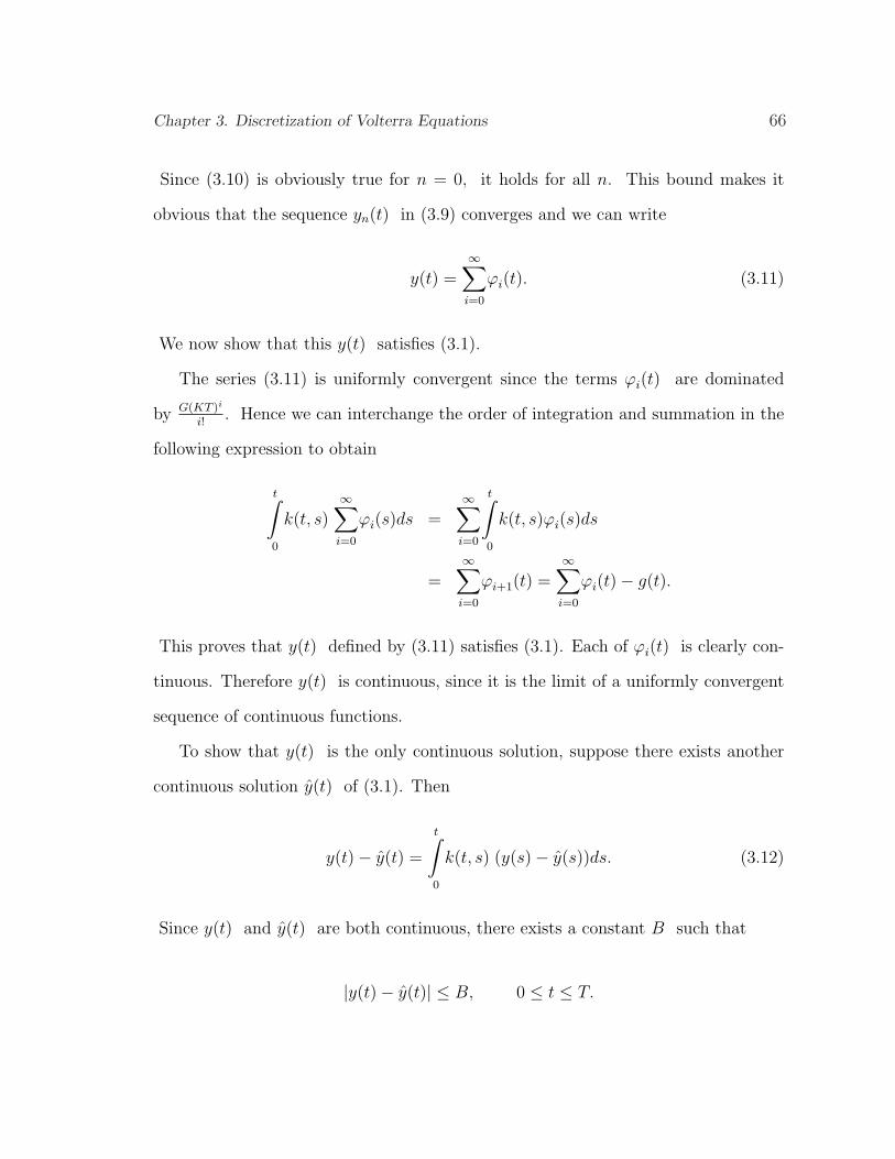
Theorem 3.1.1 If k(t, s) is continuous in 0 ≤ s ≤ t ≤ T and g(t) is continuous
in 0 ≤ t ≤ T, then (3.1) has a unique continuous solution for 0 ≤ t ≤ T.
Proof. Choose G and K such that
|g(t)| ≤ G, 0 ≤ t ≤ T,
|k(t, s)| ≤ K, 0 ≤ s ≤ t ≤ T.
We first prove by induction that
|ϕn(t)| ≤ G(Kt)n
n!, 0 ≤ t ≤ T, n = 0, 1, . . . . (3.10)
If we assume that (3.10) is true for n− 1, then from (3.8)
|ϕn(t)| ≤ G(Kt)n
(n− 1)!
t∫
0
sn−1ds ≤ G(Kt)n
n!.
Chapter 3. Discretization of Volterra Equations 66
Since (3.10) is obviously true for n = 0, it holds for all n. This bound makes it
obvious that the sequence yn(t) in (3.9) converges and we can write
y(t) =∞∑i=0
ϕi(t). (3.11)
We now show that this y(t) satisfies (3.1).
The series (3.11) is uniformly convergent since the terms ϕi(t) are dominated
by G(KT )i
i!. Hence we can interchange the order of integration and summation in the
following expression to obtain
t∫
0
k(t, s)∞∑i=0
ϕi(s)ds =∞∑i=0
t∫
0
k(t, s)ϕi(s)ds
=∞∑i=0
ϕi+1(t) =∞∑i=0
ϕi(t)− g(t).
This proves that y(t) defined by (3.11) satisfies (3.1). Each of ϕi(t) is clearly con-
tinuous. Therefore y(t) is continuous, since it is the limit of a uniformly convergent
sequence of continuous functions.
To show that y(t) is the only continuous solution, suppose there exists another
continuous solution y(t) of (3.1). Then
y(t)− y(t) =
t∫
0
k(t, s) (y(s)− y(s))ds. (3.12)
Since y(t) and y(t) are both continuous, there exists a constant B such that
|y(t)− y(t)| ≤ B, 0 ≤ t ≤ T.
Chapter 3. Discretization of Volterra Equations 67
Substituting this into (3.12)
|y(t)− y(t)| ≤ KBt, 0 ≤ t ≤ T,
and repeating the step shows that
|y(t)− y(t)| ≤ B(Kt)n
n!, 0 ≤ t ≤ T,
for any n. For large enough n , the right-hand side is arbitrarily small, so that we
must have
y(t) = y(t), 0 ≤ t ≤ T,
and there is only one continuous solution.
3.1.2 Boundedness of the Direct Quadrature Method
As we know, because of the linearity of the problem (3.1), the global error
en = y(tn)− yn
of the method satisfies an analogous Volterra difference equations
en = Tn(h) + h
n∑
l=0
wn,l kn,l el, n ≥ n0, (3.13)
where Tn(h) represents the local discretization error see [18] and it is assumed that
Tn(h) < T ∗, n ≥ n0. (3.14)
Chapter 3. Discretization of Volterra Equations 68
We will introduce the stability of the Direct Quadrature Method in the sense of
boundedness of global error. In order to show this, we first rewrite (3.13) in the
following form
en = gn +n∑
l=n0
an,l el, n ≥ n0, (3.15)
with
gn = Tn(h) +
n0−1∑
l=0
wn,l kn,l el, an,l = hwn,l kn,l.
Now by assuming that e0, e1, ..., en0−1 are given and recalling (3.15), we have the
result that the global error satisfies a Volterra difference equations of the form (2.4)
with
| gn| < g, n ≥ n0. (3.16)
Theorem 3.1.2 Assume that
i) k(t, s) ≤ 0, t ≥ t0, t0 ≤ s ≤ t,
ii) ∂k(t,s)∂t
≥ 0, t ≥ t0, t0 ≤ s ≤ t,
iii) |k(t, s)| ≤ φ(t),
iv) φ′(t) ≤ 0,
v)∞∫t0
φ(t)dt = k∗ < ∞,
vi) hφ(t0) ≤ c1.
Then the global error of the Direct Quadrature Method under consideration satis-
fies
|en| ≤ g(1 + c2k∗).
Proof. We give only the proof for the case of the TR Method since remain-
ing methods can be handled analogously. The Volterra difference equation (3.15)
Chapter 3. Discretization of Volterra Equations 69
representing the global error of the Trapezoidal Method satisfies
xn = gn +n∑
l=n0
an,l xl, n ≥ n0,
an.n 6= 1, n ≥ n0,
with
an,l =
hkn,l, 1 ≤ l ≤ n− 1h2kn,n, l = n
, n ≥ 1
and hence an+1,l ≥ an,l, 1 ≤ l ≤ n − 1. From (vi) and taking into account (iii)
and (i) one finds
h
2|kn,n| < 1,
and thus
hkn+1,n − h
2kn,n ≥ h
2kn,n > −1, n ≥ 1.
This assures that
an+1,n − an,n ≥ −1, n ≥ 1.
Then by the application of Theorem 2.2 in [39] and taking into account that
∞∑
l=1
|al+1,l| ≤ h
∞∑
l=1
|kl,l| ≤∞∫
t0
φ(t)dt = k∗,
we have that the fundamental matrix of (3.15) satisfies
n−1∑m=1
|um+1,n − um,n| ≤ 2k∗.
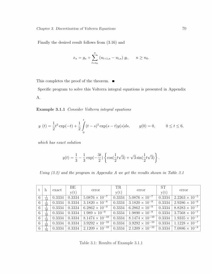
Chapter 3. Discretization of Volterra Equations 70
Finally the desired result follows from (3.16) and
xn = gn +n∑
l=n0
(ul+1,n − ul,n) gl, n ≥ n0.
This completes the proof of the theorem.
Specific program to solve this Volterra integral equations is presented in Appendix
A.
Example 3.1.1 Consider Volterra integral equations
y (t) =1
2t2 exp(−t) +
1
2
t∫
0
(t− s)2 exp(s− t)y(s)ds, y(0) = 0, 0 ≤ t ≤ 6,
which has exact solution
y(t) =1
3− 1
3exp(−3t
2)
cos(
1
2t√
3) +√
3 sin(1
2t√
3)
.
Using (3.2) and the program in Appendix A we get the results shown in Table 3.1
t h exactBEy(t)
errorTRy(t)
errorSTy(t)
error
6 110
0.3334 0.3334 5.0876× 10⁻⁷ 0.3334 5.0876× 10⁻⁷ 0.3334 2.2263× 10⁻⁵
6 120
0.3334 0.3334 3.1820× 10⁻⁸ 0.3334 3.1820× 10⁻⁸ 0.3334 2.9286× 10⁻⁶
6 130
0.3334 0.3334 6.2862× 10⁻⁹ 0.3334 6.2862× 10⁻⁹ 0.3334 8.8283× 10⁻⁷
6 140
0.3334 0.3334 1.989× 10⁻⁹ 0.3334 1.9890× 10⁻⁹ 0.3334 3.7568× 10⁻⁷
6 150
0.3334 0.3334 8.1474× 10⁻¹⁰ 0.3334 8.1474× 10⁻¹⁰ 0.3334 1.9335× 10⁻⁷
6 160
0.3334 0.3334 3.9292× 10⁻¹⁰ 0.3334 3.9292× 10⁻¹⁰ 0.3334 1.1228× 10⁻⁷
6 170
0.3334 0.3334 2.1209× 10⁻¹⁰ 0.3334 2.1209× 10⁻¹⁰ 0.3334 7.0886× 10⁻⁸
Table 3.1: Results of Example 3.1.1
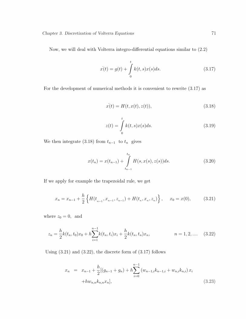
Chapter 3. Discretization of Volterra Equations 71
Now, we will deal with Volterra integro-differential equations similar to (2.2)
x´(t) = g(t) +
t∫
0
k(t, s)x(s)ds. (3.17)
For the development of numerical methods it is convenient to rewrite (3.17) as
x´(t) = H(t, x(t), z(t)), (3.18)
z(t) =
t∫
0
k(t, s)x(s)ds. (3.19)
We then integrate (3.18) from tn−1 to tn gives
x(tn) = x(tn−1) +
tn∫
tn−1
H(s, x(s), z(s))ds. (3.20)
If we apply for example the trapezoidal rule, we get
xn = xn−1 +h
2
H(t
n−1, xn−1 , zn−1) + H(tn , xn , zn)
, x0 = x(0), (3.21)
where z0 = 0, and
zn =h
2k(tn, t0)x0 + h
n−1∑i=1
k(tn, ti)xi +h
2k(tn, tn)xn, n = 1, 2, .... (3.22)
Using (3.21) and (3.22), the discrete form of (3.17) follows
xn = xn−1 +h
2[(gn−1 + gn) + h
n−1∑i=0
(wn−1,ikn−1,i + wn,ikn,i) xi
+hwn,nkn,nxn], (3.23)
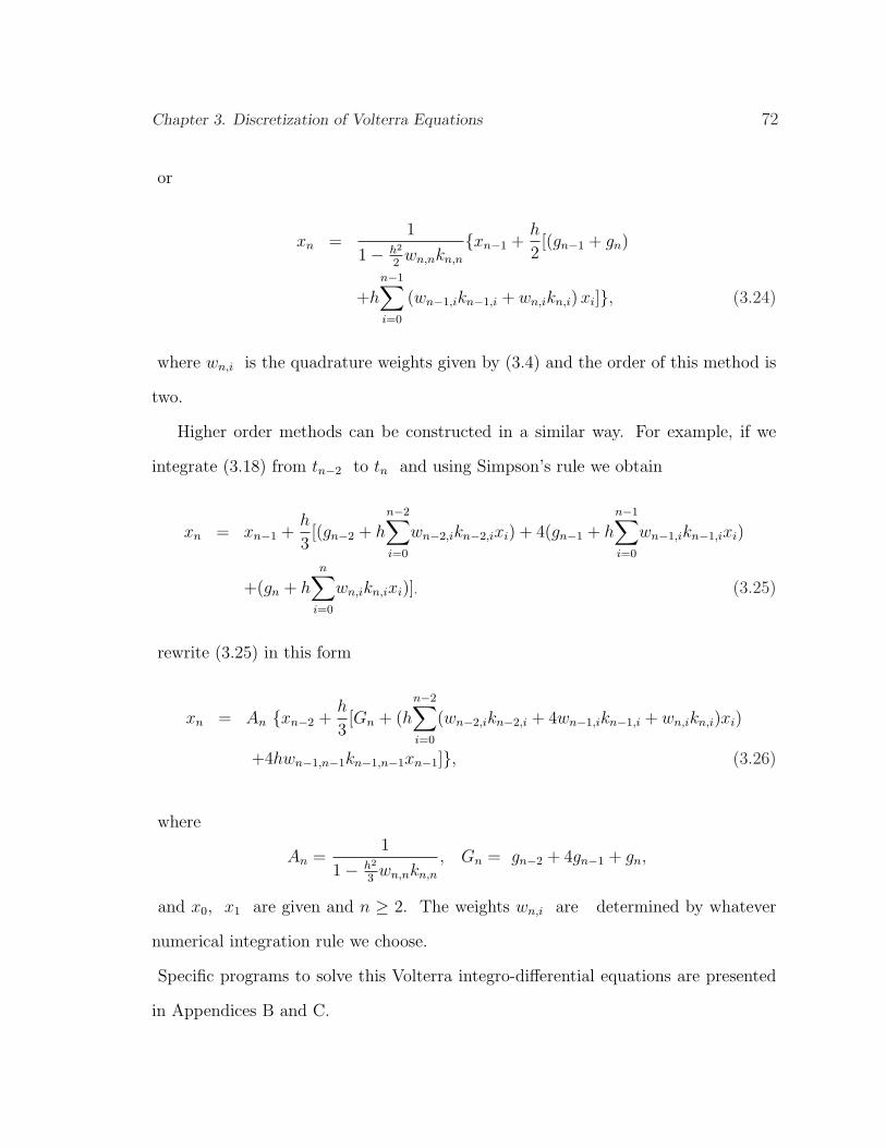
Chapter 3. Discretization of Volterra Equations 72
or
xn =1
1− h2
2wn,nkn,n
xn−1 +h
2[(gn−1 + gn)
+h
n−1∑i=0
(wn−1,ikn−1,i + wn,ikn,i) xi], (3.24)
where wn,i is the quadrature weights given by (3.4) and the order of this method is
two.
Higher order methods can be constructed in a similar way. For example, if we
integrate (3.18) from tn−2 to tn and using Simpson’s rule we obtain
xn = xn−1 +h
3[(gn−2 + h
n−2∑i=0
wn−2,ikn−2,ixi) + 4(gn−1 + h
n−1∑i=0
wn−1,ikn−1,ixi)
+(gn + h
n∑i=0
wn,ikn,ixi)], (3.25)
rewrite (3.25) in this form
xn = An xn−2 +h
3[Gn + (h
n−2∑i=0
(wn−2,ikn−2,i + 4wn−1,ikn−1,i + wn,ikn,i)xi)
+4hwn−1,n−1kn−1,n−1xn−1], (3.26)
where
An =1
1− h2
3wn,nkn,n
, Gn = gn−2 + 4gn−1 + gn,
and x0, x1 are given and n ≥ 2. The weights wn,i are determined by whatever
numerical integration rule we choose.
Specific programs to solve this Volterra integro-differential equations are presented
in Appendices B and C.
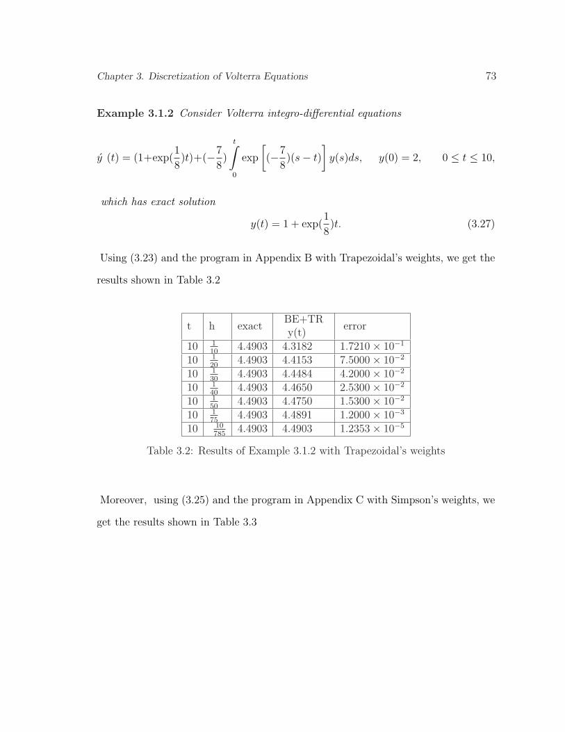
Chapter 3. Discretization of Volterra Equations 73
Example 3.1.2 Consider Volterra integro-differential equations
y (t) = (1+exp(1
8)t)+(−7
8)
t∫
0
exp
[(−7
8)(s− t)
]y(s)ds, y(0) = 2, 0 ≤ t ≤ 10,
which has exact solution
y(t) = 1 + exp(1
8)t. (3.27)
Using (3.23) and the program in Appendix B with Trapezoidal’s weights, we get the
results shown in Table 3.2
t h exactBE+TRy(t)
error
10 110
4.4903 4.3182 1.7210× 10⁻¹
10 120
4.4903 4.4153 7.5000× 10⁻²
10 130
4.4903 4.4484 4.2000× 10⁻²
10 140
4.4903 4.4650 2.5300× 10⁻²
10 150
4.4903 4.4750 1.5300× 10⁻²
10 175
4.4903 4.4891 1.2000× 10⁻³
10 10785
4.4903 4.4903 1.2353× 10⁻⁵
Table 3.2: Results of Example 3.1.2 with Trapezoidal’s weights
Moreover, using (3.25) and the program in Appendix C with Simpson’s weights, we
get the results shown in Table 3.3
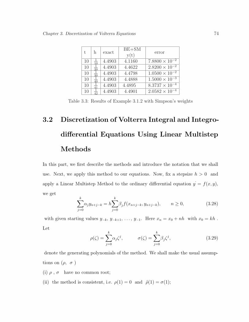
Chapter 3. Discretization of Volterra Equations 74
t h exactBE+SM
y(t)error
10 110
4.4903 4.1160 7.8800× 10⁻²
10 120
4.4903 4.4622 2.8200× 10⁻²
10 130
4.4903 4.4798 1.0500× 10⁻²
10 140
4.4903 4.4888 1.5000× 10⁻³
10 141
4.4903 4.4895 8.3737× 10⁻⁴
10 142
4.4903 4.4901 2.0582× 10⁻⁴
Table 3.3: Results of Example 3.1.2 with Simpson’s weights
3.2 Discretization of Volterra Integral and Integro-
differential Equations Using Linear Multistep
Methods
In this part, we first describe the methods and introduce the notation that we shall
use. Next, we apply this method to our equations. Now, fix a stepsize h > 0 and
apply a Linear Multistep Method to the ordinary differential equation y´ = f(x, y),
we getk∑
j=0
αjyn+j−k = h
k∑j=0
βjf(xn+j−k, yn+j−k), n ≥ 0, (3.28)
with given starting values y−k, y−k+1, . . . , y−1. Here xn = x0 + nh with x0 = kh .
Let
ρ(ζ) =k∑
j=0
αjζj, σ(ζ) =
k∑j=0
βjζj, (3.29)
denote the generating polynomials of the method. We shall make the usual assump-
tions on (ρ, σ )
(i) ρ , σ have no common root;
(ii) the method is consistent, i.e. ρ(1) = 0 and ρ(1) = σ(1);
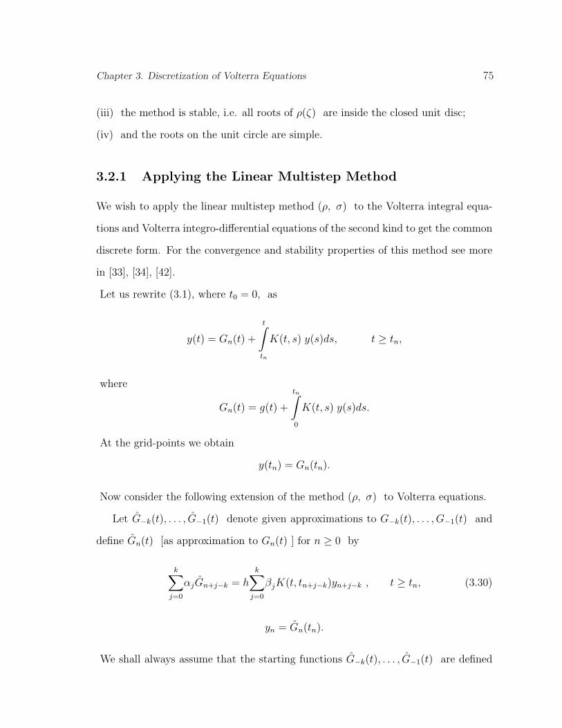
Chapter 3. Discretization of Volterra Equations 75
(iii) the method is stable, i.e. all roots of ρ(ζ) are inside the closed unit disc;
(iv) and the roots on the unit circle are simple.
3.2.1 Applying the Linear Multistep Method
We wish to apply the linear multistep method (ρ, σ) to the Volterra integral equa-
tions and Volterra integro-differential equations of the second kind to get the common
discrete form. For the convergence and stability properties of this method see more
in [33], [34], [42].
Let us rewrite (3.1), where t0 = 0, as
y(t) = Gn(t) +
t∫
tn
K(t, s) y(s)ds, t ≥ tn,
where
Gn(t) = g(t) +
tn∫
0
K(t, s) y(s)ds.
At the grid-points we obtain
y(tn) = Gn(tn).
Now consider the following extension of the method (ρ, σ) to Volterra equations.
Let G−k(t), . . . , G−1(t) denote given approximations to G−k(t), . . . , G−1(t) and
define Gn(t) [as approximation to Gn(t) ] for n ≥ 0 by
k∑j=0
αjGn+j−k = h
k∑j=0
βjK(t, tn+j−k)yn+j−k , t ≥ tn, (3.30)
yn = Gn(tn).
We shall always assume that the starting functions G−k(t), . . . , G−1(t) are defined
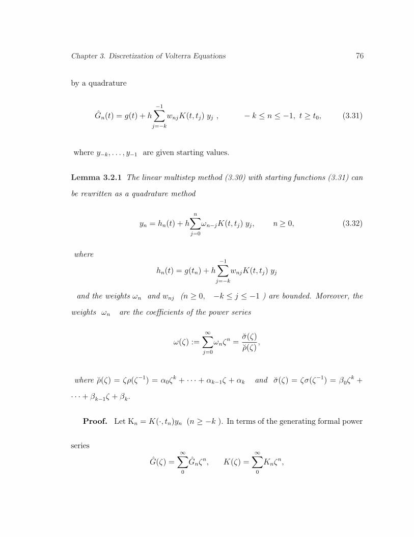
Chapter 3. Discretization of Volterra Equations 76
by a quadrature
Gn(t) = g(t) + h
−1∑
j=−k
wnjK(t, tj) yj , − k ≤ n ≤ −1, t ≥ t0, (3.31)
where y−k, . . . , y−1 are given starting values.
Lemma 3.2.1 The linear multistep method (3.30) with starting functions (3.31) can
be rewritten as a quadrature method
yn = hn(t) + h
n∑j=0
ωn−jK(t, tj) yj, n ≥ 0, (3.32)
where
hn(t) = g(tn) + h
−1∑
j=−k
wnjK(t, tj) yj
and the weights ωn and wnj (n ≥ 0, −k ≤ j ≤ −1 ) are bounded. Moreover, the
weights ωn are the coefficients of the power series
ω(ζ) :=∞∑
j=0
ωnζn =
σ(ζ)
ρ(ζ),
where ρ(ζ) = ζρ(ζ−1) = α0ζk + · · · + αk−1ζ + αk and σ(ζ) = ζσ(ζ−1) = β0ζ
k +
· · ·+ βk−1ζ + βk.
Proof. Let Kn = K(·, tn)yn (n ≥ −k ). In terms of the generating formal power
series
G(ζ) =∞∑0
Gnζn, K(ζ) =
∞∑0
Knζn,
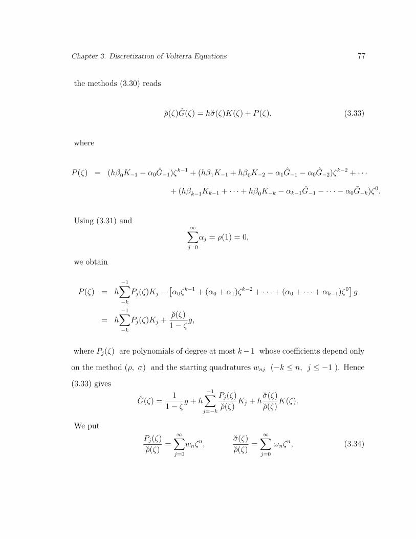
Chapter 3. Discretization of Volterra Equations 77
the methods (3.30) reads
ρ(ζ)G(ζ) = hσ(ζ)K(ζ) + P (ζ), (3.33)
where
P (ζ) = (hβ0K−1 − α0G−1)ζk−1 + (hβ1K−1 + hβ0K−2 − α1G−1 − α0G−2)ζ
k−2 + · · ·
+ (hβk−1Kk−1 + · · ·+ hβ0K−k − αk−1G−1 − · · · − α0G−k)ζ0.
Using (3.31) and∞∑
j=0
αj = ρ(1) = 0,
we obtain
P (ζ) = h
−1∑
−k
Pj(ζ)Kj −[α0ζ
k−1 + (α0 + α1)ζk−2 + · · ·+ (α0 + · · ·+ αk−1)ζ
0]g
= h
−1∑
−k
Pj(ζ)Kj +ρ(ζ)
1− ζg,
where Pj(ζ) are polynomials of degree at most k−1 whose coefficients depend only
on the method (ρ, σ) and the starting quadratures wnj (−k ≤ n, j ≤ −1 ). Hence
(3.33) gives
G(ζ) =1
1− ζg + h
−1∑
j=−k
Pj(ζ)
ρ(ζ)Kj + h
σ(ζ)
ρ(ζ)K(ζ).
We put
Pj(ζ)
ρ(ζ)=
∞∑j=0
wnζn,
σ(ζ)
ρ(ζ)=
∞∑j=0
ωnζn, (3.34)
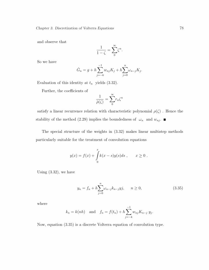
Chapter 3. Discretization of Volterra Equations 78
and observe that
1
1− ζ=
∞∑0
ζn.
So we have
Gn = g + h
−1∑
j=−k
wnjKj + h
n∑j=0
ωn−jKj.
Evaluation of this identity at tn yields (3.32).
Further, the coefficients of
1
ρ(ζ)=
∞∑0
rnζn
satisfy a linear recurrence relation with characteristic polynomial ρ(ζ) . Hence the
stability of the method (2.29) implies the boundedness of ωn and wnj.
The special structure of the weights in (3.32) makes linear multistep methods
particularly suitable for the treatment of convolution equations
y(x) = f(x) +
x∫
0
k(x− s)y(s)ds , x ≥ 0 .
Using (3.32), we have
yn = fn + h
n∑j=0
ωn−jkn−jyj, n ≥ 0, (3.35)
where
kn = k(nh) and fn = f(tn) + h
−1∑
j=−k
wnjKn−j yj.
Now, equation (3.35) is a discrete Volterra equation of convolution type.
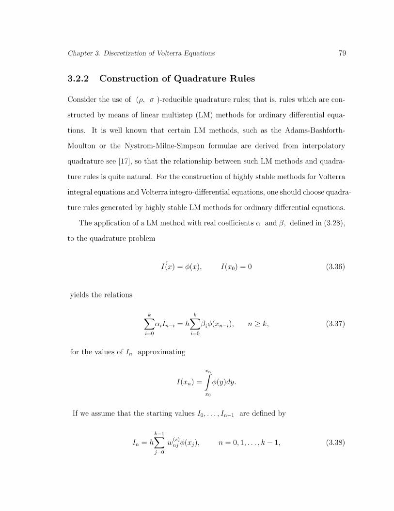
Chapter 3. Discretization of Volterra Equations 79
3.2.2 Construction of Quadrature Rules
Consider the use of (ρ, σ )-reducible quadrature rules; that is, rules which are con-
structed by means of linear multistep (LM) methods for ordinary differential equa-
tions. It is well known that certain LM methods, such as the Adams-Bashforth-
Moulton or the Nystrom-Milne-Simpson formulae are derived from interpolatory
quadrature see [17], so that the relationship between such LM methods and quadra-
ture rules is quite natural. For the construction of highly stable methods for Volterra
integral equations and Volterra integro-differential equations, one should choose quadra-
ture rules generated by highly stable LM methods for ordinary differential equations.
The application of a LM method with real coefficients α and β, defined in (3.28),
to the quadrature problem
I (x) = φ(x), I(x0) = 0 (3.36)
yields the relations
k∑i=0
αiIn−i = h
k∑i=0
βiφ(xn−i), n ≥ k, (3.37)
for the values of In approximating
I(xn) =
xn∫
x0
φ(y)dy.
If we assume that the starting values I0, . . . , In−1 are defined by
In = h
k−1∑j=0
w(s)nj φ(xj), n = 0, 1, . . . , k − 1, (3.38)
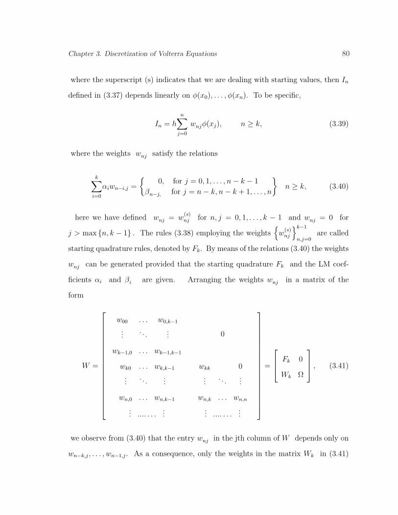
Chapter 3. Discretization of Volterra Equations 80
where the superscript (s) indicates that we are dealing with starting values, then In
defined in (3.37) depends linearly on φ(x0), . . . , φ(xn). To be specific,
In = h
n∑j=0
wnjφ(xj), n ≥ k, (3.39)
where the weights wnj satisfy the relations
k∑i=0
αiwn−i,j =
0, for j = 0, 1, . . . , n− k − 1
βn−j, for j = n− k, n− k + 1, . . . , n
n ≥ k, (3.40)
here we have defined wnj = w(s)nj for n, j = 0, 1, . . . , k − 1 and wnj = 0 for
j > max n, k − 1 . The rules (3.38) employing the weights
w(s)nj
k−1
n,j=0are called
starting quadrature rules, denoted by Fk. By means of the relations (3.40) the weights
wnj can be generated provided that the starting quadrature Fk and the LM coef-
ficients αi and βi are given. Arranging the weights wnj in a matrix of the
form
W =
w00 . . . w0,k−1
.... . .
...
wk−1,0 . . . wk−1,k−1
0
wk0 . . . wk,k−1
.... . .
...
wn,0 . . . wn,k−1
... .... . . ....
wkk 0
.... . .
...
wn,k . . . wn,n
... .... . . ....
=
Fk 0
Wk Ω
, (3.41)
we observe from (3.40) that the entry wnj in the jth column of W depends only on
wn−k,j, . . . , wn−1,j. As a consequence, only the weights in the matrix Wk in (3.41)
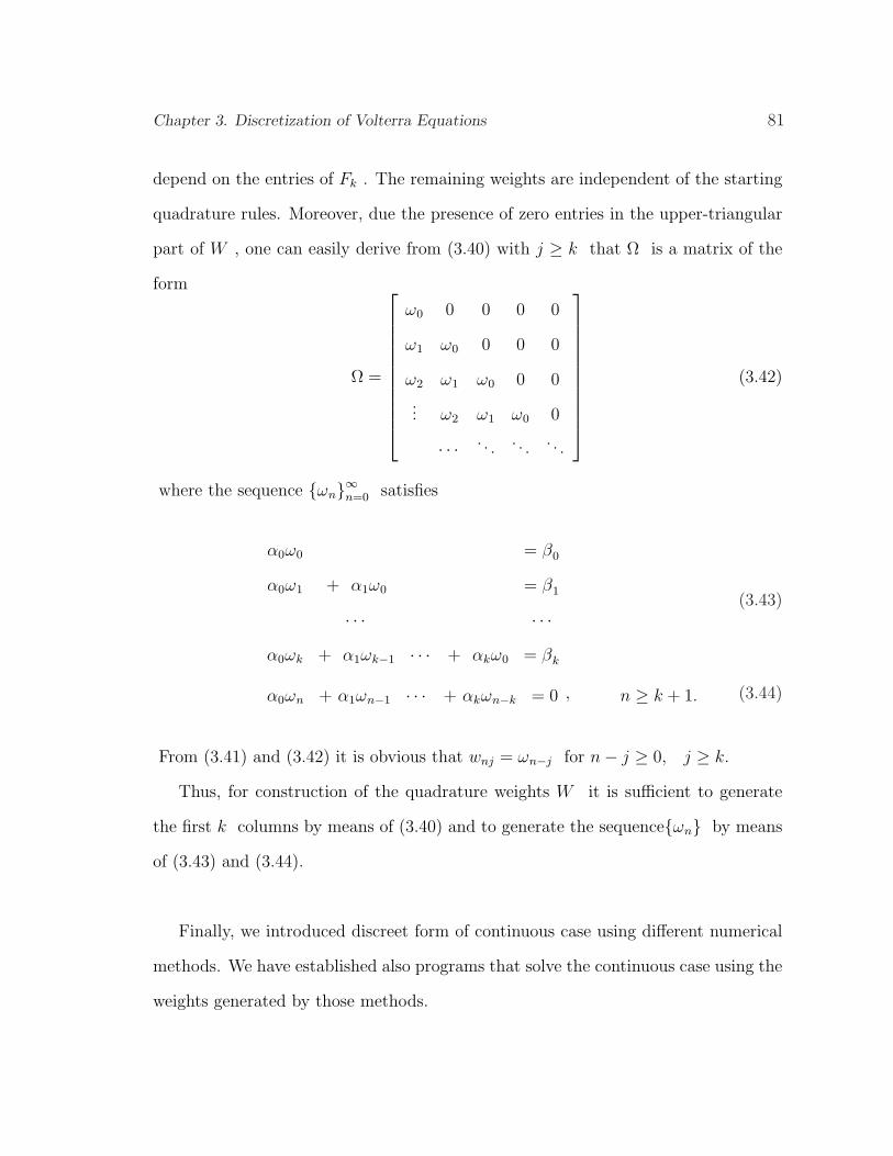
Chapter 3. Discretization of Volterra Equations 81
depend on the entries of Fk . The remaining weights are independent of the starting
quadrature rules. Moreover, due the presence of zero entries in the upper-triangular
part of W , one can easily derive from (3.40) with j ≥ k that Ω is a matrix of the
form
Ω =
ω0 0 0 0 0
ω1 ω0 0 0 0
ω2 ω1 ω0 0 0
... ω2 ω1 ω0 0
· · · . . . . . . . . .
(3.42)
where the sequence ωn∞n=0 satisfies
α0ω0 = β0
α0ω1 + α1ω0 = β1
· · · · · ·α0ωk + α1ωk−1 · · · + αkω0 = βk
(3.43)
α0ωn + α1ωn−1 · · · + αkωn−k = 0 , n ≥ k + 1. (3.44)
From (3.41) and (3.42) it is obvious that wnj = ωn−j for n− j ≥ 0, j ≥ k.
Thus, for construction of the quadrature weights W it is sufficient to generate
the first k columns by means of (3.40) and to generate the sequenceωn by means
of (3.43) and (3.44).
Finally, we introduced discreet form of continuous case using different numerical
methods. We have established also programs that solve the continuous case using the
weights generated by those methods.
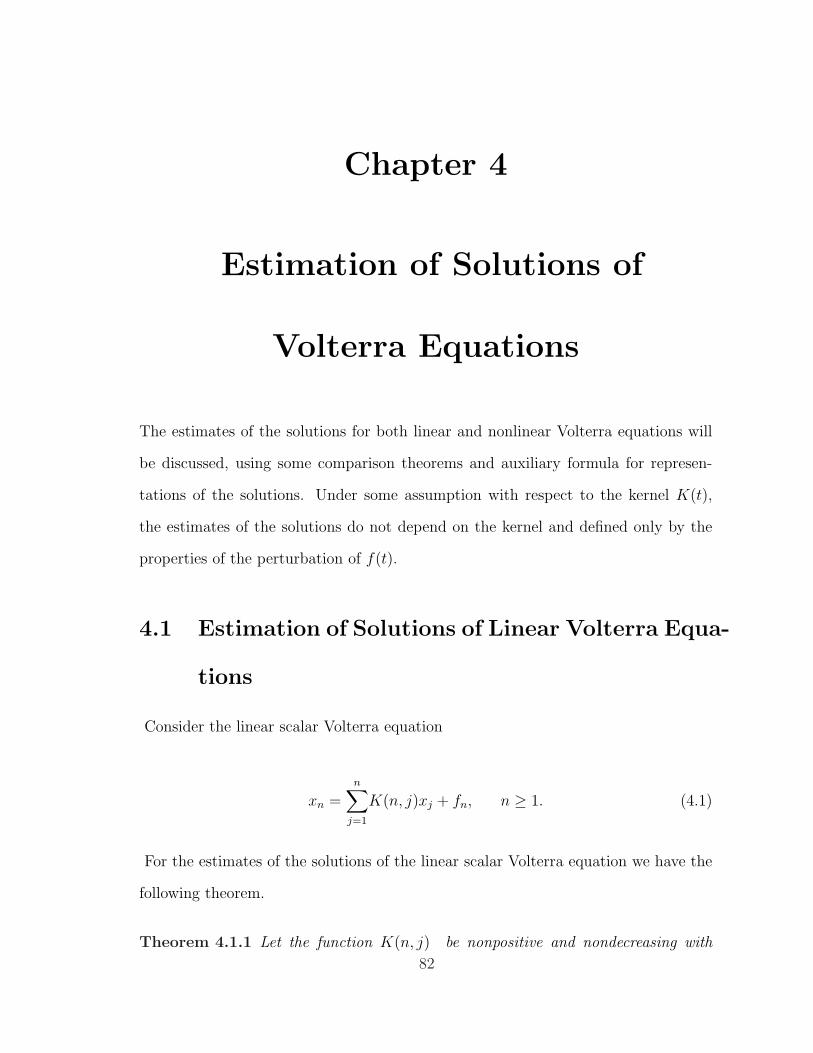
Chapter 4
Estimation of Solutions of
Volterra Equations
The estimates of the solutions for both linear and nonlinear Volterra equations will
be discussed, using some comparison theorems and auxiliary formula for represen-
tations of the solutions. Under some assumption with respect to the kernel K(t),
the estimates of the solutions do not depend on the kernel and defined only by the
properties of the perturbation of f(t).
4.1 Estimation of Solutions of Linear Volterra Equa-
tions
Consider the linear scalar Volterra equation
xn =n∑
j=1
K(n, j)xj + fn, n ≥ 1. (4.1)
For the estimates of the solutions of the linear scalar Volterra equation we have the
following theorem.
Theorem 4.1.1 Let the function K(n, j) be nonpositive and nondecreasing with
82
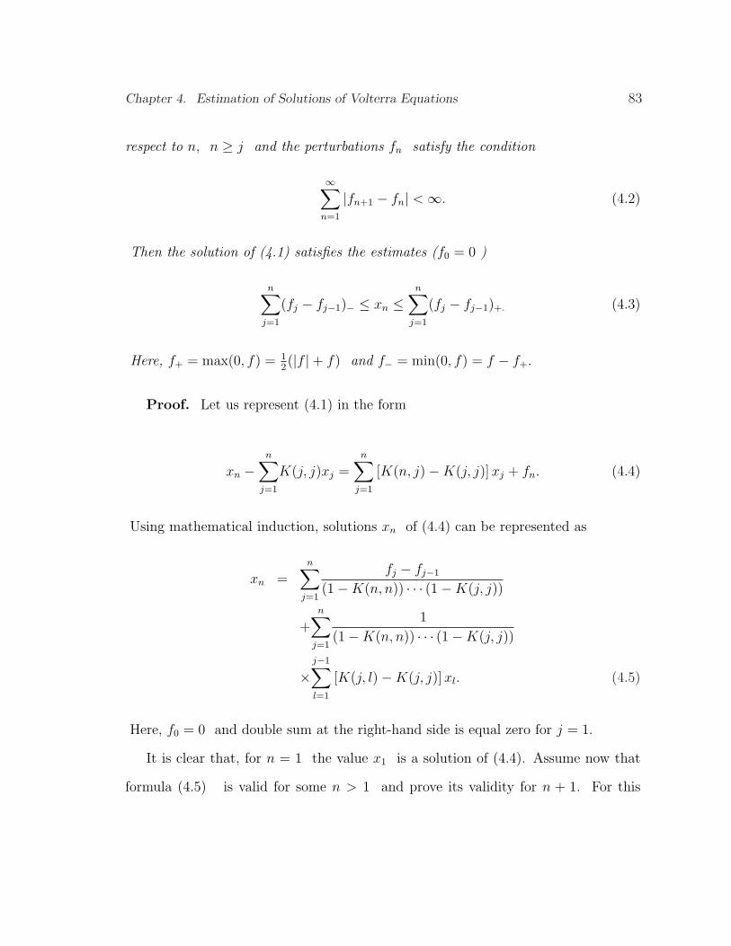
Chapter 4. Estimation of Solutions of Volterra Equations 83
respect to n, n ≥ j and the perturbations fn satisfy the condition
∞∑n=1
|fn+1 − fn| < ∞. (4.2)
Then the solution of (4.1) satisfies the estimates (f0 = 0 )
n∑j=1
(fj − fj−1)− ≤ xn ≤n∑
j=1
(fj − fj−1)+. (4.3)
Here, f+ = max(0, f) = 12(|f |+ f) and f− = min(0, f) = f − f+.
Proof. Let us represent (4.1) in the form
xn −n∑
j=1
K(j, j)xj =n∑
j=1
[K(n, j)−K(j, j)] xj + fn. (4.4)
Using mathematical induction, solutions xn of (4.4) can be represented as
xn =n∑
j=1
fj − fj−1
(1−K(n, n)) · · · (1−K(j, j))
+n∑
j=1
1
(1−K(n, n)) · · · (1−K(j, j))
×j−1∑
l=1
[K(j, l)−K(j, j)] xl. (4.5)
Here, f0 = 0 and double sum at the right-hand side is equal zero for j = 1.
It is clear that, for n = 1 the value x1 is a solution of (4.4). Assume now that
formula (4.5) is valid for some n > 1 and prove its validity for n + 1. For this
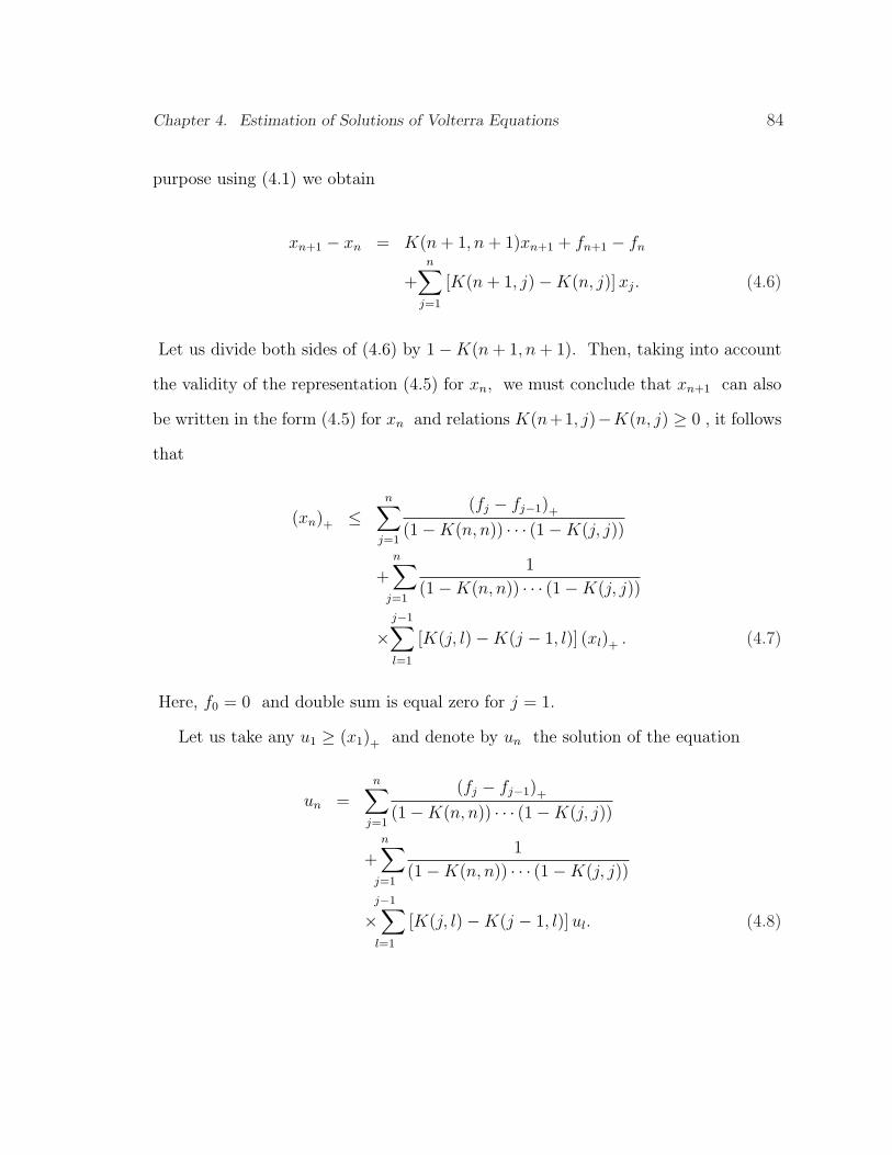
Chapter 4. Estimation of Solutions of Volterra Equations 84
purpose using (4.1) we obtain
xn+1 − xn = K(n + 1, n + 1)xn+1 + fn+1 − fn
+n∑
j=1
[K(n + 1, j)−K(n, j)] xj. (4.6)
Let us divide both sides of (4.6) by 1−K(n + 1, n + 1). Then, taking into account
the validity of the representation (4.5) for xn, we must conclude that xn+1 can also
be written in the form (4.5) for xn and relations K(n+1, j)−K(n, j) ≥ 0 , it follows
that
(xn)+ ≤n∑
j=1
(fj − fj−1)+
(1−K(n, n)) · · · (1−K(j, j))
n
+∑
j=1
1
(1−K(n, n)) · · · (1−K(j, j))
×j−1∑
l=1
[K(j, l)−K(j − 1, l)] (xl)+ . (4.7)
Here, f0 = 0 and double sum is equal zero for j = 1.
Let us take any u1 ≥ (x1)+ and denote by un the solution of the equation
un =n∑
j=1
(fj − fj−1)+
(1−K(n, n)) · · · (1−K(j, j))
n
+∑
j=1
1
(1−K(n, n)) · · · (1−K(j, j))
j−1
×∑
l=1
[K(j, l)−K(j − 1, l)] ul. (4.8)
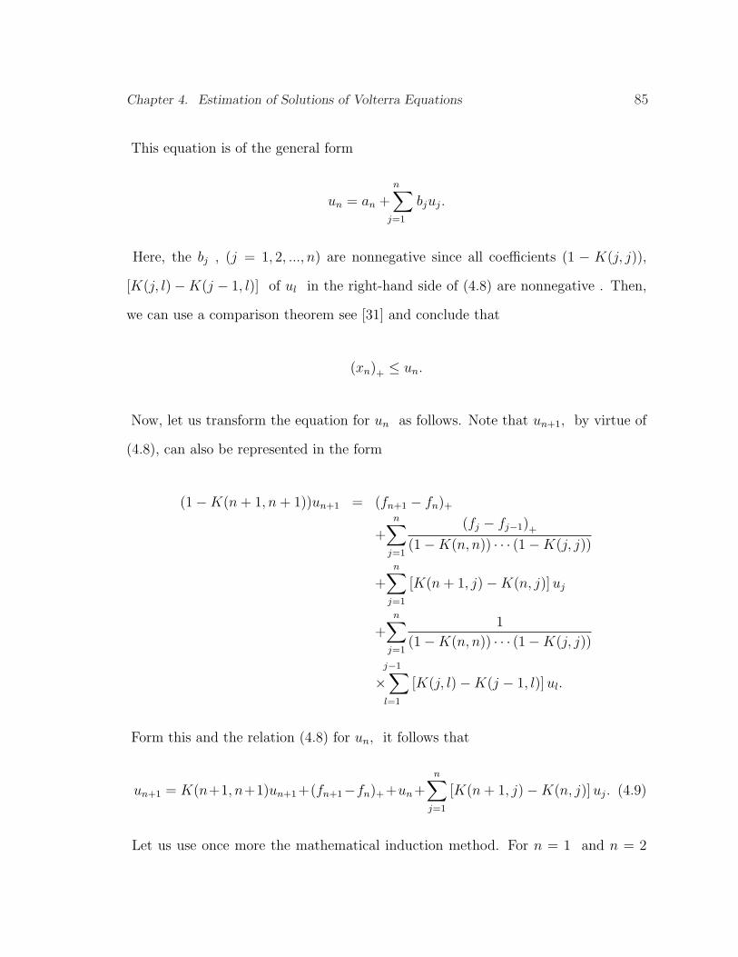
Chapter 4. Estimation of Solutions of Volterra Equations 85
This equation is of the general form
un = an
n
+∑
j=1
bjuj.
Here, the bj , (j = 1, 2, ..., n) are nonnegative since all coefficients (1 − K(j, j)),
[K(j, l)−K(j − 1, l)] of ul in the right-hand side of (4.8) are nonnegative . Then,
we can use a comparison theorem see [31] and conclude that
(xn)+ ≤ un.
Now, let us transform the equation for un as follows. Note that un+1, by virtue of
(4.8), can also be represented in the form
(1−K(n + 1, n + 1))un+1 = (fn+1 − fn)+
+n∑
j=1
(fj − fj−1)+
(1−K(n, n)) · · · (1−K(j, j))
+n∑
j=1
[K(n + 1, j)−K(n, j)] uj
+n∑
j=1
1
(1−K(n, n)) · · · (1−K(j, j))
j−1
×∑
l=1
[K(j, l)−K(j − 1, l)] ul.
Form this and the relation (4.8) for un, it follows that
un+1 = K(n+1, n+1)un+1+(fn+1−fn)++un+n∑
j=1
[K(n + 1, j)−K(n, j)] uj. (4.9)
Let us use once more the mathematical induction method. For n = 1 and n = 2
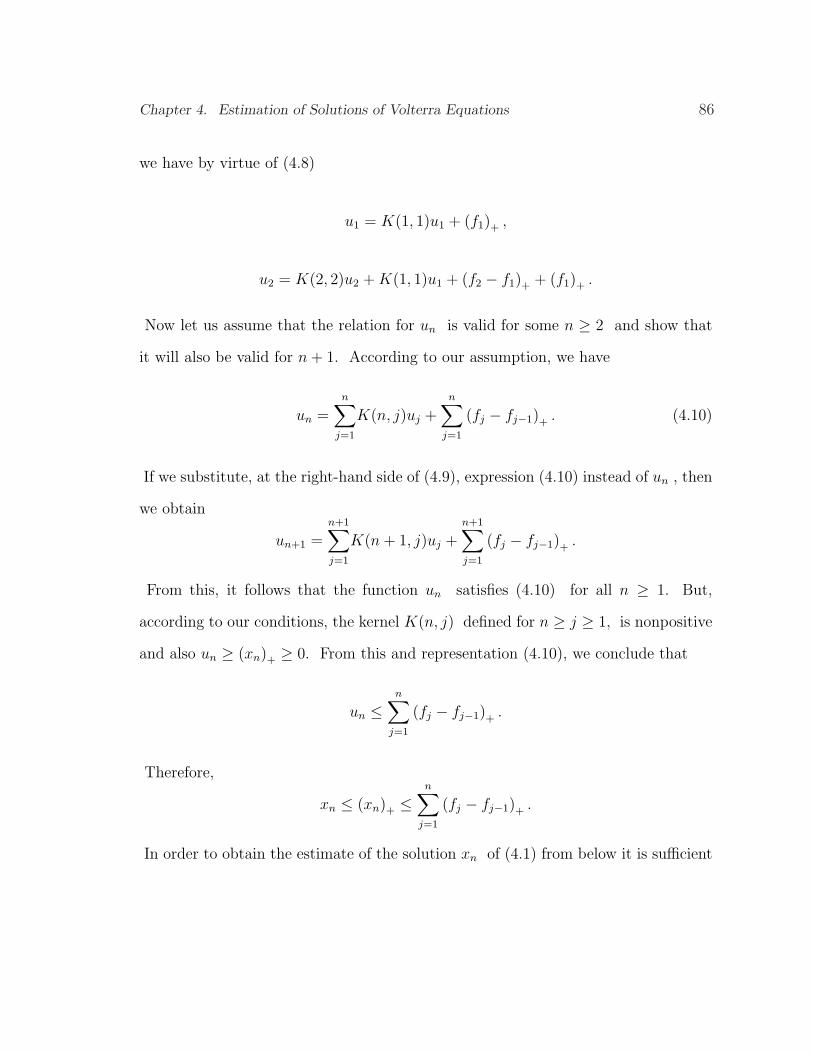
Chapter 4. Estimation of Solutions of Volterra Equations 86
we have by virtue of (4.8)
u1 = K(1, 1)u1 + (f1)+ ,
u2 = K(2, 2)u2 + K(1, 1)u1 + (f2 − f1)+ + (f1)+ .
Now let us assume that the relation for un is valid for some n ≥ 2 and show that
it will also be valid for n + 1. According to our assumption, we have
un =n∑
j=1
K(n, j)uj +n∑
j=1
(fj − fj−1)+ . (4.10)
If we substitute, at the right-hand side of (4.9), expression (4.10) instead of un , then
we obtain
un+1 =n+1∑j=1
K(n + 1, j)uj +n+1∑j=1
(fj − fj−1)+ .
From this, it follows that the function un satisfies (4.10) for all n ≥ 1. But,
according to our conditions, the kernel K(n, j) defined for n ≥ j ≥ 1, is nonpositive
and also un ≥ (xn)+ ≥ 0. From this and representation (4.10), we conclude that
un ≤n∑
j=1
(fj − fj−1)+ .
Therefore,
xn ≤ (xn)+ ≤n∑
j=1
(fj − fj−1)+ .
In order to obtain the estimate of the solution xn of (4.1) from below it is sufficient
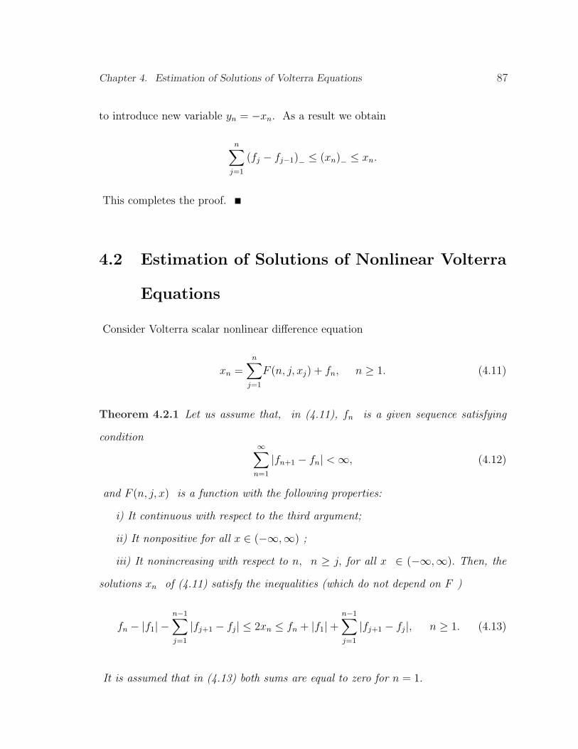
Chapter 4. Estimation of Solutions of Volterra Equations 87
to introduce new variable yn = −xn. As a result we obtain
n∑j=1
(fj − fj−1)− ≤ (xn)− ≤ xn.
This completes the proof.
4.2 Estimation of Solutions of Nonlinear Volterra
Equations
Consider Volterra scalar nonlinear difference equation
xn =n∑
j=1
F (n, j, xj) + fn, n ≥ 1. (4.11)
Theorem 4.2.1 Let us assume that, in (4.11), fn is a given sequence satisfying
condition∞∑
n=1
|fn+1 − fn| < ∞, (4.12)
and F (n, j, x) is a function with the following properties:
i) It continuous with respect to the third argument;
ii) It nonpositive for all x ∈ (−∞,∞) ;
iii) It nonincreasing with respect to n, n ≥ j, for all x ∈ (−∞,∞). Then, the
solutions xn of (4.11) satisfy the inequalities (which do not depend on F )
fn − |f1| −n−1∑j=1
|fj+1 − fj| ≤ 2xn ≤ fn + |f1|+n−1∑j=1
|fj+1 − fj|, n ≥ 1. (4.13)
It is assumed that in (4.13) both sums are equal to zero for n = 1.
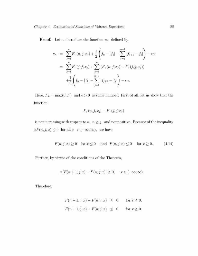
Chapter 4. Estimation of Solutions of Volterra Equations 88
Proof. Let us introduce the function un defined by
un =n∑
j=1
F+(n, j, xj) +1
2
(fn − |f1| −
n−1∑j=1
|fj+1 − fj|)− εn
=n∑
j=1
F+(j, j, xj) +n∑
j=1
(F+(n, j, xj)− F+(j, j, xj))
+1
2
(fn − |f1| −
n−1∑j=1
|fj+1 − fj|)− εn.
Here, F+ = max(0, F ) and ε > 0 is some number. First of all, let us show that the
function
F+(n, j, xj)− F+(j, j, xj)
is nonincreasing with respect to n, n ≥ j, and nonpositive. Because of the inequality
xF (n, j, x) ≤ 0 for all x ∈ (−∞,∞), we have
F (n, j, x) ≥ 0 for x ≤ 0 and F (n, j, x) ≤ 0 for x ≥ 0. (4.14)
Further, by virtue of the conditions of the Theorem,
x [F (n + 1, j, x)− F (n, j, x)] ≥ 0, x ∈ (−∞,∞).
Therefore,
F (n + 1, j, x)− F (n, j, x) ≤ 0 for x ≤ 0,
F (n + 1, j, x)− F (n, j, x) ≤ 0 for x ≥ 0.
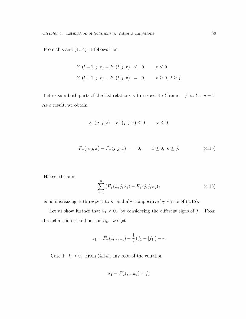
Chapter 4. Estimation of Solutions of Volterra Equations 89
From this and (4.14), it follows that
F+(l + 1, j, x)− F+(l, j, x) ≤ 0, x ≤ 0,
F+(l + 1, j, x)− F+(l, j, x) = 0, x ≥ 0, l ≥ j.
Let us sum both parts of the last relations with respect to l froml = j to l = n− 1.
As a result, we obtain
F+(n, j, x)− F+(j, j, x) ≤ 0, x ≤ 0,
F+(n, j, x)− F+(j, j, x) = 0, x ≥ 0, n ≥ j. (4.15)
Hence, the sumn∑
j=1
(F+(n, j, xj)− F+(j, j, xj)) (4.16)
is nonincreasing with respect to n and also nonpositive by virtue of (4.15).
Let us show further that u1 < 0, by considering the different signs of f1. From
the definition of the function un, we get
u1 = F+(1, 1, x1) +1
2(f1 − |f1|)− ε.
Case 1: f1 > 0. From (4.14), any root of the equation
x1 = F (1, 1, x1) + f1
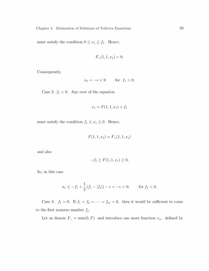
Chapter 4. Estimation of Solutions of Volterra Equations 90
must satisfy the condition 0 ≤ x1 ≤ f1. Hence,
F+(1, 1, x1) = 0.
Consequently,
u1 = −ε < 0 for f1 > 0.
Case 2: f1 < 0. Any root of the equation
x1 = F (1, 1, x1) + f1
must satisfy the condition f1 ≤ x1 ≤ 0. Hence,
F (1, 1, x1) = F+(1, 1, x1)
and also
−f1 ≥ F (1, 1, x1) ≥ 0.
So, in this case
u1 ≤ −f1 +1
2(f1 − |f1|)− ε = −ε < 0, for f1 < 0.
Case 3: f1 = 0. If f1 = f2 = · · · = fm = 0, then it would be sufficient to come
to the first nonzero number fj.
Let us denote F− = min(0, F ) and introduce one more function υn, defined by
Chapter 4. Estimation of Solutions of Volterra Equations 91
the relation
υn = −n∑
j=1
F−(j, j, xj)−n∑
j=1
(F−(n, j, xj)− F−(j, j, xj))
−1
2
(fn − |f1| −
n−1∑j=1
|fj+1 − fj|)− εn,
for n ≥ 1, ε > 0. Let us check that υ1 < 0, by using the same arguments as above
for the proof that u1 < 0. We have
υ1 = −F−(1, 1, x1)− 1
2(f1 − |f1|)− ε.
If f1 > 0, then any root of the equation
x1 = F (1, 1, x1) + f1
must satisfy the condition 0 ≤ x1 ≤ f1. Hence,
F−(1, 1, x1) = F (1, 1, x1)
and, moreover,
−f1 ≤ F−(1, 1, x1) ≤ 0, i.e., 0 ≤ −F−(1, 1, x1) ≤ f1.
Therefore,
υ1 ≤ −f1 +1
2(f1 − |f1|)− ε = −ε < 0.
Chapter 4. Estimation of Solutions of Volterra Equations 92
If f1 < 0, then any root of the equation
x1 = F (1, 1, x1) + f1
will satisfy the condition f1 ≤ x1 ≤ 0, i.e., F−(1, 1, x1) = 0. It means that υ =
−ε < 0. As a result, for all cases, υ1 = −ε < 0. Let us show that the function
F−(n, j, xj)− F (j, j, xj),
is a nondecreasing function of n. Since the function xF (n, j, x) is nondecreasing for
all x ∈ (−∞,∞) , we can conclude that
x [F (n + 1, j, x)− F (n, j, x)] ≥ 0.
Therefore,
F (n + 1, j, x)− F (n, j, x) ≥ 0, x ≥ 0.
Besides,
F−(n, j, x) = F (n, j, x), x ≥ 0.
It means that
F−(n + 1, j, x)− F−(n, j, x) ≥ 0.
From this, it follows that the function
F−(n, j, x)− F−(j, j, x) ≥ 0, n ≥ j,
Chapter 4. Estimation of Solutions of Volterra Equations 93
is a nonnegative and nondecreasing function of n, n ≥ j. Hence, the sum
n∑j=1
[F−(n, j, x)− F−(j, j, x)] (4.17)
is nondecreasing with respect to n and nonnegative. Let us remark also that, form
the definitions of the functions un, υn and (4.11), it follows that
xn =n∑
j=1
(F+(n, j, xj)− F−(n, j, xj)) + fn = un − υn. (4.18)
Further, the sum (4.16) is nonincreasing with respect to n , then because of (4.18),
we get
un+1 − un ≤ F+(n + 1, n + 1, xn+1)− ε +1
2(fn+1 − fn − |fn+1 − fn|)
≤ F+(n + 1, n + 1, xn+1)− ε
= F+(n + 1, n + 1, un+1 − υn+1)− ε. (4.19)
Similarly, because the sum (4.17) is nondecreasing with respect to n , we obtain for
the difference υn+1 − υn the estimate
υn+1 − υn ≤ −F−(n + 1, n + 1, xn+1)− ε
= −F−(n + 1, n + 1, un+1 − υn+1)− ε. (4.20)
As a result, we have obtained that u1 < 0 , υ1 < 0 and both inequalities (4.19),
(4.20) are valid. Now, we have three possibilities.
Chapter 4. Estimation of Solutions of Volterra Equations 94
Case 1: If u1 < 0 , υ1 < 0 for all n ≥ 1 then by virtue of (4.18) and conditions
F+(n, j, xj) ≥ 0, F−(n, j, xj) ≤ 0,
we obtain
1
2
(fn − |f1| −
n−1∑j=1
|fj+1 − fj|)− εn ≤ un ≤ un − υn = xn ≤ υn
≤ 1
2
(fn + |f1|+
n−1∑j=1
|fj+1 − fj|)
+ εn.
From this and arbitrariness of ε > 0, we derive the estimates (4.13).
Now consider two cases when inequalities un < 0 and υn < 0 are not valid for
all n > 1.
Case 2: Assume that there exists a first moment n0 > 1 such that
un < 0, 1 ≤ n ≤ n0, un0+1 ≥ 0, υn ≤ 0, 1 ≤ n ≤ n0,
but un0+1 − υn0+1 ≥ 0. Then we have
un0+1 − un0 ≥ 0.
On the other hand, by virtue of (4.19) and (4.14)
un0+1 − un0 ≤ F+(n0 + 1, n0 + 1, un0+1 − υn0+1)− ε = −ε < 0.
Case 3: Consider now the second possible case when there exists a first moment
Chapter 4. Estimation of Solutions of Volterra Equations 95
n0 > 1 such that
υn < 0, 1 ≤ n ≤ n0, υn0+1 ≥ 0, un ≤ 0, 1 ≤ n ≤ n0,
and besides υn0+1 − un0+1 ≥ 0. Then we have
υn0+1 − υn0 ≥ 0.
On the other hand, due to (4.20) and (4.14)
υn0+1 − υn0 ≤ −F−(n0 + 1, n0 + 1, un0+1 − υn0+1)− ε = −ε.
Since Cases 2 and 3 lead to contradictions, the remaining Case 1 proves the estimates
(4.13) and proof of the theorem complete.
Chapter 5
Conclusion and Further Research
We introduced linear difference equations, which occur in numerous settings and
forms, both in mathematics itself and its applications. Mainly we concentrated on
Volterra difference equations of the second type.
Volterra difference equations of the second type have been discussed in many
aspects. With different types of kernels, stability, periodicity, and boundedness have
been studied. Results on the boundedness and stability of solutions of these equations
based on the growth properties of the fundamental matrix and the resolvent matrix.
Using these properties we found an explicit criteria. In the coming days, we expect
generalization of some results work on the implicit form. Also, nonhomogeneous cases
of Volterra type will be discussed in terms of their perturbations.
Also, how to change continuous case to a discrete case presented through out
numerical methods. Specific programs have been constructed with different methods
that solve both Volterra integrals and intgro-differential equations. For the future,
we should look for quadrature rules generated by specific weights to construct highly
stable methods.
We defined estimations of the solutions, of both cases linear and nonlinear not
depending on the kernel. These estimations are defined only by the properties of the
perturbation terms.
96

In conclusion we suggest the construction of an algorithm that specify all in-
formation that are needed, stability, periodicity, boundedness, and estimations, by
simply entering kernel and perturbation function of Volterra difference equations of
the second kind.
97
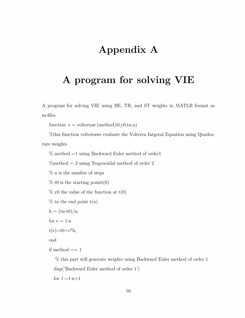
Appendix A
A program for solving VIE
A program for solving VIE using BE, TR, and ST weights in MATLB format as
m-files.
function s = volterraw (method,t0,y0,tn,n)
%this function volterrawe evaluate the Volterra Intgeral Equation using Quadra-
ture weights
% method =1 using Backward Euler method of order1
%method = 2 using Trapezoidal method of order 2
% n is the number of steps
% t0 is the starting pointt(0)
% y0 the value of the function at t(0)
% tn the end point t(n)
h = (tn-t0)/n;
for e = 1:n
t(e)=t0+e*h;
end
if method == 1
% this part will generate weights using Backward Euler method of order 1
disp(’Backward Euler method of order 1’)
for l =1:n+1
98
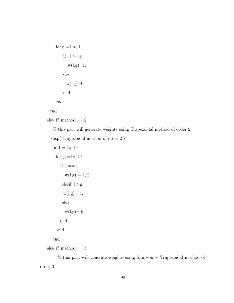
for g =1:n+1
if l >=g
w(l,g)=1;
else
w(l,g)=0;
end
end
end
else if method ==2
% this part will generate weights using Trapezoidal method of order 2
disp(’Trapezoidal method of order 2’)
for l = 1:n+1
for g =1:n+1
if l == j
w(l,g) = 1/2;
elseif l >g
w(l,g) =1;
else
w(l,g)=0;
end
end
end
else if method ==3
% this part will generate weights using Simpson + Trapezoidal method of
order 3
99
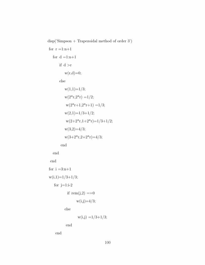
disp(’Simpson + Trapezoidal method of order 3’)
for r =1:n+1
for d =1:n+1
if d >r
w(r,d)=0;
else
w(1,1)=1/3;
w(2*r,2*r) =1/2;
w(2*r+1,2*r+1) =1/3;
w(2,1)=1/3+1/2;
w(2+2*r,1+2*r)=1/3+1/2;
w(3,2)=4/3;
w(3+2*r,2+2*r)=4/3;
end
end
end
for i =3:n+1
w(i,1)=1/3+1/3;
for j=1:i-2
if rem(j,2) ==0
w(i,j)=4/3;
else
w(i,j) =1/3+1/3;
end
end
100
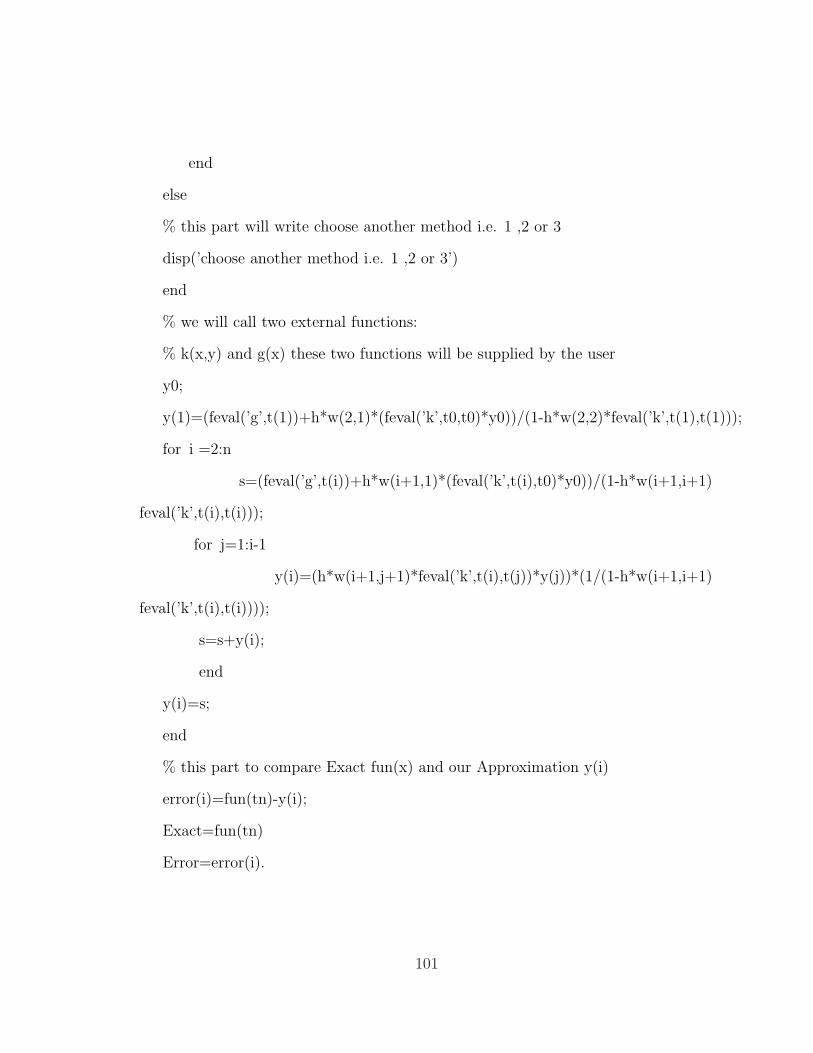
end
else
% this part will write choose another method i.e. 1 ,2 or 3
disp(’choose another method i.e. 1 ,2 or 3’)
end
% we will call two external functions:
% k(x,y) and g(x) these two functions will be supplied by the user
y0;
y(1)=(feval(’g’,t(1))+h*w(2,1)*(feval(’k’,t0,t0)*y0))/(1-h*w(2,2)*feval(’k’,t(1),t(1)));
for i =2:n
s=(feval(’g’,t(i))+h*w(i+1,1)*(feval(’k’,t(i),t0)*y0))/(1-h*w(i+1,i+1)
feval(’k’,t(i),t(i)));
for j=1:i-1
y(i)=(h*w(i+1,j+1)*feval(’k’,t(i),t(j))*y(j))*(1/(1-h*w(i+1,i+1)
feval(’k’,t(i),t(i))));
s=s+y(i);
end
y(i)=s;
end
% this part to compare Exact fun(x) and our Approximation y(i)
error(i)=fun(tn)-y(i);
Exact=fun(tn)
Error=error(i).
101
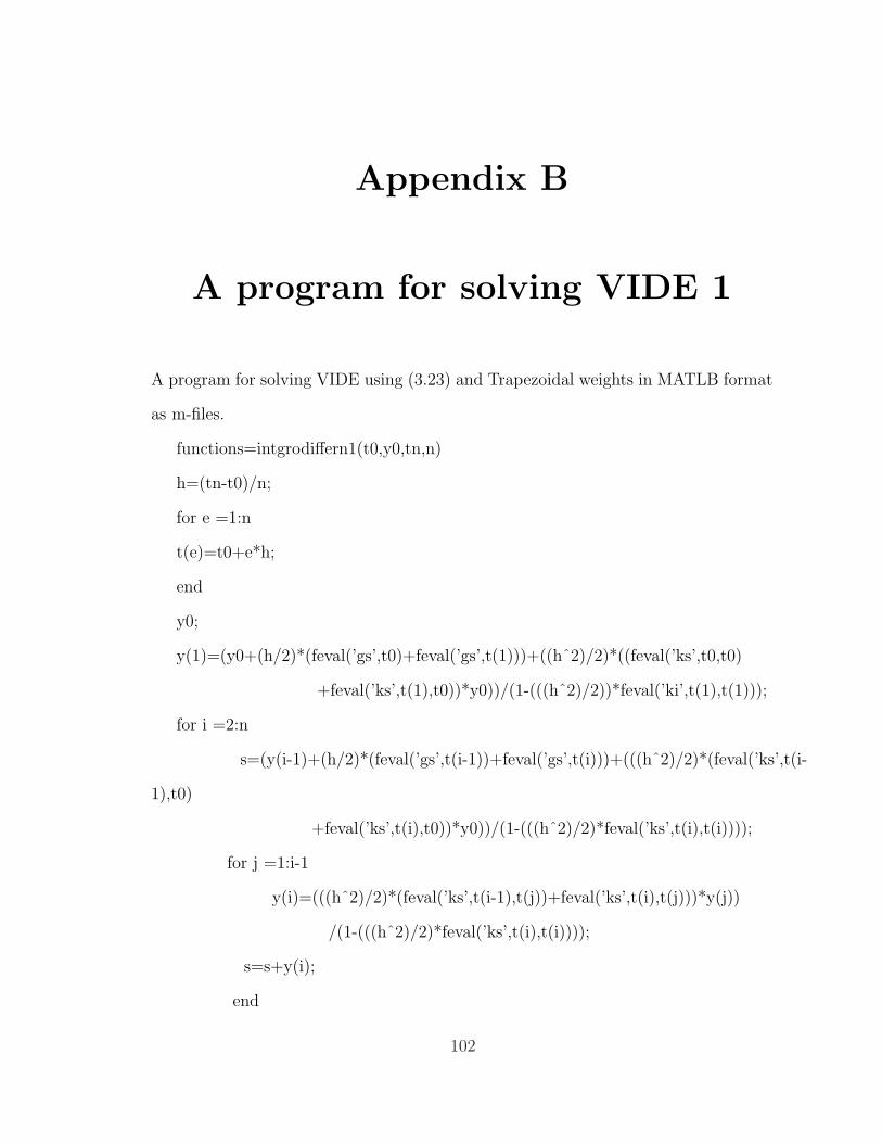
Appendix B
A program for solving VIDE 1
A program for solving VIDE using (3.23) and Trapezoidal weights in MATLB format
as m-files.
functions=intgrodiffern1(t0,y0,tn,n)
h=(tn-t0)/n;
for e =1:n
t(e)=t0+e*h;
end
y0;
y(1)=(y0+(h/2)*(feval(’gs’,t0)+feval(’gs’,t(1)))+((hˆ2)/2)*((feval(’ks’,t0,t0)
+feval(’ks’,t(1),t0))*y0))/(1-(((hˆ2)/2))*feval(’ki’,t(1),t(1)));
for i =2:n
s=(y(i-1)+(h/2)*(feval(’gs’,t(i-1))+feval(’gs’,t(i)))+(((hˆ2)/2)*(feval(’ks’,t(i-
1),t0)
+feval(’ks’,t(i),t0))*y0))/(1-(((hˆ2)/2)*feval(’ks’,t(i),t(i))));
for j =1:i-1
y(i)=(((hˆ2)/2)*(feval(’ks’,t(i-1),t(j))+feval(’ks’,t(i),t(j)))*y(j))
/(1-(((hˆ2)/2)*feval(’ks’,t(i),t(i))));
s=s+y(i);
end
102
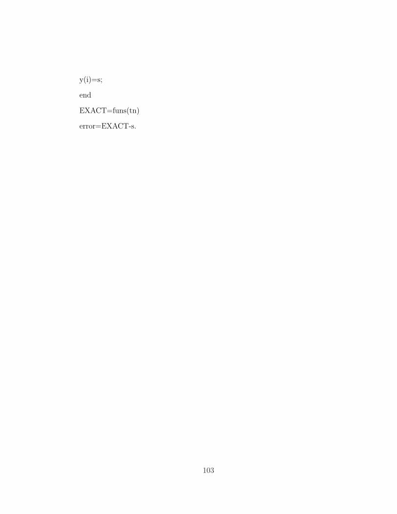
y(i)=s;
end
EXACT=funs(tn)
error=EXACT-s.
103
Appendix C
A program for solving VIDE 2
A program for solving VIDE using (3.25) and Simpson’s weights in MATLAB formate
as m-files.
functions =intgrodiffern2(t0,y0,y1,tn,n)
%this function intgro evaluate the Volterra Intgero-differential Equation using BE
weights
% t0 is the starting point t(0)
% y0 the value of the function at t(0)
%y1 the value of the function at t(1)
% tn the end point t(n)
% n is the number of steps
h=(tn-t0)/n;
for e=1:n+5;
t(e)=t0+e*h;
end
y0;
y(1)=y1;
y(2)=(1/(1-((hˆ2)/3)*feval(’ks’,t(2),t(2))))*(y0+((h/3)*(feval(’gs’,t0)
+4*feval(’gs’,t(1))+feval(’gs’,t(2))))+((h/3)*h*(4*feval(’ks’,t(1),t(1))
+feval(’ks’,t(2),t(1)))*y(1))+((h/3)*h*(feval(’ks’,t0,t0)+4*feval(’ks’,t(1),t0)
104
+feval(’ks’,t(2),t0))*y0));
for i=3:n
s=(1/(1-((hˆ2)/3)*feval(’ks’,t(i),t(i))))*(y(i-2)+((h/3)*(feval(’gs’,t(i-2))
+4*feval(’gs’,t(i-1))+feval(’gs’,t(i)))+((h/3)*h*(4*feval(’ks’,t(i-1),t(i-1))
+feval(’ks’,t(i),t(i-1)))*y(i-1))+((h/3)*h*(feval(’ks’,t(i-2),t0)+4*feval(’ks’,t(i-
1),t0)
+feval(’ks’,t(i),t0))*y0)));
for j=1:i-2
y(i)=(1/(1-((hˆ2)/3)*feval(’ks’,t(i),t(i))))*((h/3)*h*(feval(’ks’,t(i-
2),t(j))+4*feval(’ks’,t(i-1),t(j))
+feval(’ks’,t(i),t(j))))*y(j);
s=s+y(i);
end
y(i)=s;
end
Exact=funs(tn)
error=funs(tn)-y(i).
105
References
[1] P. Agarwal and Patricia J. Wong, Advanced Topics in Difference Equations,Kulwer Academic Puiblishers, 1997.
[2] L. Babai and T. Lengyel, A convergence for recurrent sequences with applicationsto the partition lattice, Analysis 12 (1992), 109–119.
[3] H. Brunner, Iterated collocation methods and their discretizations for Volterraintegral equations, SIAM J. Numer. Anal. 21 (1984), 1132–1145.
[4] Burden and J. Faires, Numerical Analysis, 6. ed., International Thomson Pub-lishing company, Pacific Grove, 1997.
[5] T. A. Burton, Volterra Integral and Differential Equations, Academic Press, NewYork, 1983.
[6] C. Corduneanu and I. W. Sandberg, Volterra Equations and Applications, 2000.
[7] M. R. Crisci, Stability analysis of discrete recurrence equations of Volterra typewith degenerate kernels, Journal of Math. Analysis and Applications 162 (1991),49–62.
[8] M. R. Crisci, V. B. Kolmanovskii, E. Russo, and A.Vecchio, Boundedness ofdiscrete Volterra equations, J. Math. Anal. Appl. 211 (1997), 106–130.
[9] , Stability of the difference Volterra equations: Direct Liapunov methodand numerical procedure, Computers Math. Applic. 36 (1998), 77–97.
[10] , Asymptotic properties of solutions of Volterra difference equations withfinite linear part, Dynamic Systems and Application 8 (1999), 1–20.
[11] L. M. Delves and J. L. Mohamed, Computational Methods for Integral Equations,Combridge University Press, 1985.
[12] S. Elaydi, Periodicity and stability of linear Volterra difference systems, J. Math.anal. Appl. 181 (1994), 483–492.
[13] , An Introduction to Difference Equations, 2. ed., Springer-Verlag, NewYork, 1999.
[14] P. W. Eloe, M. N. Islam, and Y. N. Raffoul, Advences of uniform asymptoticstability in nonlinear Volterra discrete systems, Journal of Difference Equations,(to be appear).
[15] C. Gear, Numerical Initial Value Problems in Ordinary Differential Equations,Prentice-Hall, London, 1971.
[16] M. I. Gil and Rigoberto Medina, Boundedness of solution of matrix nonlinearVolterra difference equations, 7 (2002), 19–22.
[17] P. Henrici, Discrete Variable Methods in Ordinary Differential Equations, JohnWiley & Sons, New York, 1962.
[18] , Error Propagation for Difference Methods, Robert E. Krieger Publishingcompany, New York, 1977.
[19] E. Isaacson and H. Keller, Analysis of Numerical Methods, John Wiley & Sons,New York, 1966.
[20] M. N. Islam and Y. N. Raffoul, Stability properties of linear Volterra integro-differential equations with nonlinear perturbation, (to be appear).
[21] , Uniform asymptotic stability in linear Volterra difference equations,Panamerican mathematical Journal 11 (2001), 61–73.
[22] A. J. Jerri, Linear Difference Equations with Discrete Transform Methods, Kul-wer Academic Puiblishers, 1996.
[23] L. Johnson and R. Riess, Numerical Analysis, 2. ed., Addison-Wesley Publishingcompany, New York, 1982.
[24] W. G. Kelley and A. C. Peterson, Difference Equations: An Introduction withApplications, Academic Press, New York, 2001.
[25] T. M. Khandaker and Y. N. Raffoul, Stability properties of linear Volterra dis-crete systems with nonlinear perturbation, journal of difference equations andapplications, 8 (2002), 857–874.
[26] V. B. Kolmanovskii, Asymptotic properties of solutions for discrete Volterraequations, personal communication.
[27] , On the exponential stability of some Volterra difference equations, Au-tomation and Remote Control 58 (1997), No. 7.
107
[28] V. B. Kolmanovskii and N. P. Kosreva, One method of Liapunov functionalsconstruction, proceedings of dynamic systems and Applications 3 (2001), 343–350.
[29] V. B. Kolmanovskii and A. I. Mataso, Duality theory in filtering problem fordiscrete Volterra equations, 15th Triennial World Congress, Barcelona, Spain.
[30] V. B. Kolmanovskii and J. P. Richard, Estimation of solutions of Volterra dif-ference equations, J. Math. Anal. Appl. 273 (2002), 618–626.
[31] V. Lakshmikantham and D. Trigiante, Theory of Difference Equations: Numer-ical Methods and Applications, Academic Press, New York, 1988.
[32] H. Lauwerier, Mathematical Models of Epidemcs, Math. Centrum, Amsterdam,1981.
[33] P. Linz, Analytical and Numerical Methods for Volterra Equations, SIAM,Philadelphia, 1985.
[34] Ch. Lubich, On the stability of linear multistep methods for Volterra convolutionequations, IMA Journal of Numerical Analysis 3 (1983), 439–465.
[35] R. Medina, Boundedness of perturbed Volterra discrete equations, Proceeding ofDynamic Systems and Application 3 (2001), 417–424.
[36] E. J. Muth, Transform Methods with Application to Engineering and OperationsResearch, Prentice-Hall Inc, London, 1977.
[37] Y. N. Raffoul, Uniform asymptotic stability in linear Volterra systems with non-linear perturbation, Intl. Journal of Difference Equations, (to be appear).
[38] Y. N. Raffoul and Youssef M. Dib, Boundedness and stability in nonlinear dis-crete systems with nonlinear perturbation, Intl. Journal of Difference Equations,(to be appear).
[39] A. Vecchio, Stability of direct quadrature methods for system of Volterra integralequations, Dynam. Systems Appl. 7 (1998), 501–518.
[40] , On the resolvent kernel of Volterra discrete equations, Functional Dif-ferential Eqautions 6 (1999), 187–197.
[41] , Volterra discrete equations: summability of the fundamental matrix,Journal of Numer. Math. 89 (2001), 783–794.
[42] P. H. M. Wolkenfelt, The construction of reducible quadrature rules for Volterraintegral and integro-differential equations, IMA Journal of Numerical Analysis 2(1982), 131–152.
108
[43] S. Zhang, The unique existence of periodic solutions of linear Volterra differenceequations, J. Math. anal. Appl. 193 (1995), 419–430.
109
Vita
- Said Ali Al-Garni.
- Born in Thoqba, in March 1974, in Saudi Arabia.
- Received B. S. of Science degree in Mathematics in May 1997.
- Joined Mathematical Science Department as a Graduate Assistant.
- Received M. Sc. of Science Degree in Mathematics in April 2003.
- Homepage: http://users.kfupm.edu.sa/math/garnis/
- E mail: [email protected]