Numerical study of the trapped and extended Bose-Hubbard ...
97
Institute for Theoretical Physics Master thesis Numerical study of the trapped and extended Bose-Hubbard models Author: Tommaso Comparin Supervisor: Prof. dr. Cristiane Morais Smith (ITP, Utrecht University) Co-supervisors: Marco Di Liberto MSc (ITP, Utrecht University) Dr. Federico Becca (CNR-IOM and ISAS-SISSA) August 2013
Transcript of Numerical study of the trapped and extended Bose-Hubbard ...

Institute for Theoretical Physics
Master thesis
Numerical study of the trapped
and extended Bose-Hubbard
models
Author:
Tommaso Comparin
Supervisor:
Prof. dr. Cristiane Morais Smith
(ITP, Utrecht University)
Co-supervisors:
Marco Di Liberto MSc(ITP, Utrecht University)
Dr. Federico Becca
(CNR-IOM and ISAS-SISSA)
August 2013

Abstract
The Bose-Hubbard model describes the physics of a systemof bosonic ultracold atoms in an optical lattice, in which a phasetransition is present between a superfluid phase and a Mott insu-lator one. The exact solution of this Hamiltonian is only feasibleto find the ground-state of small systems, while other techniques(as mean-field schemes or quantum Monte Carlo) are necessaryto study systems of larger size.
As a first application, we study the trapped model – relevantfor the comparison with current experiments – through an in-homogeneous mean-field scheme. We describe some signaturesof the phase crossover between superfluid and Mott insulator.In particular, the visibility of the quasimomentum distributionshows some kinks as a function of the lattice depth; we describethese features and we link them with the ones observed in otherworks in the literature.
As a second application, we use quantum Monte Carlo tech-niques to study the one-dimensional Bose-Hubbard model withlong-range interactions and we focus on the appearance of theHaldane insulating phase, distinguishable from the Mott onethrough the presence of non-local hidden order. Non-local corre-lation functions are also used to describe the difference betweenthe superfluid phase and the Mott insulator one.
i

Contents
Abstract i
Introduction 1
1 Bose-Hubbard Model 4
1.1 Lattice Hamiltonian . . . . . . . . . . . . . . . . . . . . . . . 41.2 Wannier functions and harmonic approximation . . . . . . . . 71.3 Band structure calculation of J . . . . . . . . . . . . . . . . . 91.4 Homogeneous phase diagram . . . . . . . . . . . . . . . . . . 121.5 Inhomogeneous system: shell structure . . . . . . . . . . . . . 151.6 Time-of-flight measurements . . . . . . . . . . . . . . . . . . . 171.7 Extended Bose-Hubbard model . . . . . . . . . . . . . . . . . 18
2 Visibility in the trapped system 22
2.1 Visibility . . . . . . . . . . . . . . . . . . . . . . . . . . . . . 232.2 First observation of kinks in V . . . . . . . . . . . . . . . . . 242.3 Interpretation by QMC in 1D . . . . . . . . . . . . . . . . . . 252.4 Other QMC studies . . . . . . . . . . . . . . . . . . . . . . . 282.5 Kinks in the triangular lattice . . . . . . . . . . . . . . . . . . 30
3 Numerical techniques 32
3.1 Exact diagonalization . . . . . . . . . . . . . . . . . . . . . . 333.2 Mean-field approaches . . . . . . . . . . . . . . . . . . . . . . 35
3.2.1 Bogoliubov approximation . . . . . . . . . . . . . . . . 353.2.2 Site-decoupled mean-field approach . . . . . . . . . . . 373.2.3 Gutzwiller ansatz . . . . . . . . . . . . . . . . . . . . . 383.2.4 Numerical scheme . . . . . . . . . . . . . . . . . . . . 41
3.3 Validation of the mean-field scheme . . . . . . . . . . . . . . . 423.3.1 Homogeneous system . . . . . . . . . . . . . . . . . . . 433.3.2 Inhomogeneous system . . . . . . . . . . . . . . . . . . 45
3.4 Quantum Monte Carlo . . . . . . . . . . . . . . . . . . . . . . 533.4.1 Variational Monte Carlo . . . . . . . . . . . . . . . . . 533.4.2 Green’s Function Monte Carlo . . . . . . . . . . . . . 57
ii
CONTENTS iii
4 Trapped model: mean-field results 62
4.1 1D system . . . . . . . . . . . . . . . . . . . . . . . . . . . . . 624.2 2D system . . . . . . . . . . . . . . . . . . . . . . . . . . . . . 67
5 Extended model: QMC results 73
5.1 Validation of the GFMC scheme . . . . . . . . . . . . . . . . 745.2 Results . . . . . . . . . . . . . . . . . . . . . . . . . . . . . . . 76
5.2.1 Insulating phases . . . . . . . . . . . . . . . . . . . . . 765.2.2 Superfluid phase . . . . . . . . . . . . . . . . . . . . . 79
Conclusions 82
Acknowledgements 85

Introduction
The research in the field of cold atoms in optical lattices has attracted muchattention in the last decade, due to major experimental and theoretical ad-vances. This is the study of particles moving in a “crystal of light” (theoptical lattice), created by interfering laser beams. There is a direct cor-respondence with the case of electrons in the ionic lattice (as in a typicalsolid state system), and in fact some identical approaches are often used,as for instance the tight-binding model. However, the optical lattice set-uphas some advantages with respect to solid state systems. First, light-crystalstructures are very clean and host few defects; second, in a cold-atomicsystem the parameters of the model are usually highly tunable, whereas insolid state they are set by chemical properties of the components. The largedegree of control experimentally achievable on the parameters of the latticehas opened the idea of using cold atoms in optical lattices to realize quan-tum simulators, i.e. experiments designed to simulate specific models fromcondensed matter and reproduce their physical behaviour, following ideasby Feynman [1].
A successful description for a system of bosonic atoms in an optical lat-tice is the Bose-Hubbard model, theoretically introduced in 1989 by MatthewFisher and collaborators [2]. The phase diagram of this system at zero tem-perature includes a superfluid phase and a Mott-insulator one, separated bya quantum phase transition. In 1998 it was proposed that this model can besimulated in cold-atomic experiments [3], and in 2002 Markus Greiner andcollaborators have observed the first signature of the Mott phase transitionin such a set-up [4]. Together with the choice of new systems to study,recently there have also been advances in the precision of measurements,leading for instance to a resolution and control of the system at the level ofa single-site [5, 6, 7].
In this thesis we have studied two realizations of the Bose-Hubbardmodel. In the first case we have added an external inhomogeneous potentialto the original (homogeneous) model; this allows a closer comparison withexperiments, in which a confining potential is required to keep the atomsinside a limited region of space. Because of the inhomogeneity, the systemis not in a single global phase but it includes different domains. In particu-
1

INTRODUCTION 2
lar, for an isotropic harmonic potential one can observe the formation of astructure of concentric shells of different phases. The structure and size ofthese shells – depending on a competition between the trapping potentialand the interactions between particles – are relevant to explain some exper-imental results, as the coherence measurements that are obtained throughtime-of-flight imaging.
As a second case, we have studied the presence of non-local order insome phases of the Bose-Hubbard model. Inspired by research about spinsystems started around 30 years ago, in 2006 it has been proposed [8] that ina one-dimensional Bose-Hubbard model a long-range repulsion can stabilizea topological phase (the Haldane insulator). The phase characterization ofthe system takes place by measuring some non-local correlation functionsand it has been later used in the numerical or analytic studies of similarmodels [9, 10, 11]. Parts of this description have been recently confirmedin experiments with bosonic atoms [12], while the case of fermions is onlydescribed theoretically [13], by now.
As for other strongly-correlated systems, there is no exact analytic solu-tion for the ground state of the Bose-Hubbard model; for this reason, thishas been frequently used as a playground to introduce and test new solu-tion techniques (exact or approximated). In this thesis we make use of twotechniques. The first one is a site-decoupled mean-field technique (corre-sponding to the Gutzwiller ansatz). This is computationally inexpensiveand allows the study of large and inhomogeneous systems, i.e. the experi-mentally relevant ones. However, it gives only an approximate solution, andin particular the description of the Mott insulator phase does not accountcorrectly for fluctuations. The quantum Monte Carlo (QMC) approach in-cludes a wide class of techniques, some of which are statistically exact (in thesense that they give unbiased estimates of physical quantities). In partic-ular, QMC schemes for bosonic problems without frustration are generallynot affected by the so called sign problem, that makes the study of fermionicsystems more complex. Two common QMC schemes for the study of theBose-Hubbard model are the Green’s Function QMC (used in this thesis)and the Worm algorithm [14] (in the framework of the Path Integral QMC[15]). We also mention the Density Matrix Renormalization Group (DMRG)technique [16] (not used here), that provides precise results in the study of1D systems. Recently, this approach has been reinterpreted as part of theclass of Matrix Product State schemes [17], and connected to the broaderclass of Tensor Network techniques [18].
We also mention here some of the extensions of the Bose-Hubbard modelthat have been proposed and studied, both theoretically and experimentally.When the optical lattice includes a site-dependent disorder term, this canlead to a localization of the bosons and to the appearance of another phase

INTRODUCTION 3
(the Bose glass); this was theoretically predicted in 1989 [2] and its firstexperimental signature was observed in 2007 [19]. In the context of time-dependent models, the use of Floquet theory [20] has introduced a way toobtain effective Hamiltonians with peculiar features, as a rescaling of thetunneling parameter or the inclusion of correlated hopping processes; notethat the original Hamiltonians can be realized in experiments by “shak-ing” the lattice, i.e. through a perturbation that is periodic in time. An-other example in the context of time-dependent models is reported in Ref.[21], where the resulting effective Hamiltonian includes an artificial magneticfield. This is linked to a class of systems that have been actively studiedin the last years, namely the ones including an artificial gauge field for coldatoms in optical lattices [22]. A suitable design of the experimental set-upallows to simulate these models, in which the neutral atoms feel the effect ofa gauge field in a way analogous to the Aharonov-Bohm effect for chargedparticles in electromagnetic fields. The directions of research in this subjectinclude the characterization of quantum Hall states, the simulation of (pos-sibly non-Abelian) lattice gauge theories, and even the study of topologicalfield theory or Quark confinement in Quantum Chromodynamics.
General reviews about ultracold atoms in optical lattices can be foundin Refs [23, 24, 25, 26], while the reviews in Refs [27] and [22] are aboutsystems of dipolar bosonic atoms and artificial gauge fields, respectively.
The outline of this thesis is the following: we begin in chapter 1 with ageneral description of the Bose-Hubbard model, in which the lattice Hamilto-nian is derived and its parameters are linked to the microscopic ones; we alsodescribe the phase diagram of the homogeneous system and how it changeswhen an external trapping potential is included. In chapter 2, we introducethe motivation for our mean-field study of the trapped system. This comesfrom to the observation of certain features in the visibility of the quasi-momentum distribution (a measure of the coherence of the system); thesefeatures are observed both in experimental and numerical results. Somenumerical methods that can be used to study the Bose-Hubbard model aredescribed in chapter 3. We explain the reason why the exact diagonaliza-tion of the Hamiltonian is not feasible for large systems, and we describe amean-field approach (valid for the homogeneous and trapped system) andsome QMC techniques. In chapter 4 we present the results of our mean-fieldstudy of trapped systems in 1D and 2D; in particular, we show the den-sity profiles for different choices of the parameters and the correspondingresults for the visibility. In chapter 5 we show the results of our QMC studyof the one-dimensional model with nearest-neighbour interactions and wepresent the characterization of some of the phases of the system, based onthe measurement of non-local correlation functions. In the end we summa-rize the conclusions of this work and give an outlook about possible futuredevelopments.

Chapter 1
Bose-Hubbard Model
In this chapter we describe some general features of the Bose-Hubbard modeland introduce some quantities that are used to characterize its phases. Insection 1.1 we show how the Hamiltonian can be derived as a low temper-ature effective model for a gas of ultracold atoms in an optical lattice; insections 1.2 and 1.3 we give more details about how the parameters of themodel depend on the microscopic ones; in sections 1.4 and 1.5 we describethe theoretical phase diagram of the system and how it explains the shellstructure of the inhomogeneous model; in section 1.6 we describe the typi-cal measurements performed in experiments; in section 1.7 we describe anextended version of the Bose-Hubbard model, relevant to describe dipolarparticles.
1.1 Lattice Hamiltonian
In this section we consider a system of cold atoms in continuous space andwe show how the addition of a potential generated through interfering laserbeams leads to a lattice model.
We consider the following second-quantized Hamiltonian in terms of thebosonic atomic field ψ(x)
H =
∫
dx ψ†(x)
(
− ~2
2m∇2 + VOL(x) + VT (x)− µ
)
ψ(x)+
+1
2
∫
dx dx′ ψ†(x)ψ†(x′)V (x− x′)ψ(x′)ψ(x),
(1.1)
in which m is the atomic mass. This Hamiltonian includes a single-particlepart (kinetic term, optical lattice potential VOL, trapping potential VT andchemical potential µ) and an interaction potential V (x − x′). We considerthe s-wave scattering approximation (valid for low energy scattering) and
4

CHAPTER 1. BOSE-HUBBARD MODEL 5
Figure 1.1: Examples of laser beams interfering to create the optical latticepotential. The resulting potential is a 2D array of 1D tubes (a), or a 3Dlattice of tightly confining harmonic oscillator potentials on each site (b).Figure extracted from Ref. [23].
we replace the general interaction potential with a contact interaction
V (x− x′) =4πas~
2
mδ(x− x′), (1.2)
in which as is the s-wave scattering length. The trapping potential hasgenerally the following form
VT (r) =m
2
3∑
j=1
(
ωTj xj)2, (1.3)
in which the three trap frequencies ωTj are not necessarily the same.The optical lattice potential VOL(x) is produced through the interfer-
ence of counter-propagating laser beams [23]. In the simple case of a cubiclattice1, the resulting potential is
VOL(x) =3∑
j=1
Vj,0 sin2(kLxj), (1.4)
1More complicated lattice structures can be obtained by putting the laser beams atcertain angles; see for instance Ref. [28].

CHAPTER 1. BOSE-HUBBARD MODEL 6
where kL ≡ 2π/λ and λ is the wave length of the laser beams generating thelattice. Each one of the terms Vj,0 sin
2(kLxj) is obtained by superimposingtwo polarized electromagnetic waves (see Fig. 1.1); the induced atomic dipolecouples with the external electric field and this results in the confinement ofthe atoms around certain positions, forming a lattice with spacing a = λ/2.
Since this potential is periodic in space, the fields can be expanded interms of Bloch’s wave functions ψn,k(x), that have the same periodicityof the lattice and are labeled through the band index n and the quasi-momentum k. Starting from the Bloch basis, we introduce the Wannierbasis through
Wn(x− xj) =1√V
∑
k∈BZψn,k(x)e
−ik·(x−xj), (1.5)
where xj is a lattice site, BZ represents the first Brillouin zone and V isthe volume. From now on, we only consider the Wannier state with lowestenergy: W (x − xj) ≡ W0(x − xj). This assumption is justified when thegap to the first excited state W1 is large if compared with the energy scaleof interactions and of thermal fluctuations, and this is generally satisfied inpractice [3]. Given the Wannier basis, the fields ψ and ψ† can be expandedas the following sums over all the lattice sites
ψ†(x) =∑
j
W ∗(x− xj) b†j ,
ψ(x) =∑
j
W (x− xj) bj ,(1.6)
where b†i (bi) is the operator that creates (annihilates) a particle in the state
W (x − xi). While rewriting the Hamiltonian in terms of the operators biand b†i , we make use of the following assumptions:
1. the hopping processes between sites that are not nearest-neighboursare negligible w.r.t. the ones between nearest neighbours (this will bejustified in section 1.3);
2. the interaction between particles on different sites is much smaller thanthe on-site one, and can be neglected. In section 1.7, the model withlonger-ranged interactions will be described.
Given these assumptions, the original Hamiltonian (Eq. 1.1) reduces to theBose-Hubbard Hamiltonian:
H = −J∑
〈i,j〉b†i bj +
U
2
∑
i
b†i b†i bibi +
∑
i
(ǫi − µ)b†i bi, (1.7)

CHAPTER 1. BOSE-HUBBARD MODEL 7
where 〈i, j〉 denotes nearest neighbouring sites and where we have defined
J =
∫
dx W ∗(x− xi)
(
− ~2
2m∇2 + VOL(x)
)
W (x− xj), (1.8)
U =4πas~
2
m
∫
dx |W (x)|4, (1.9)
ǫi =
∫
dx VT (x)|W (x− xi)|2 ≈ VT (xi). (1.10)
Note that the expressions for the hopping coefficient J and for the on-site re-pulsion U are exact, but we will need some approximations (see sections 1.2and 1.3) to evaluate them explicitly. The last step of Eq. (1.10) is based onthe assumption that the characteristic length on which the trapping poten-tial changes is much larger than the spatial extent of the Wannier functionW (x− xi).
1.2 Wannier functions and harmonic approxima-
tion
In this section we derive an approximate expression for the Wannier func-tions of the lattice and we use it to estimate the value of U , the on-siterepulsive interaction coefficient.
We consider the lattice potential in Eq. (1.4); this potential has the prop-erty of being separable, i.e. it can be written as the sum of terms dependingonly on one component of x. Therefore the corresponding Wannier functionW (x) in each site can be factorized as
W (x) = w1(x)w2(y)w3(z). (1.11)
The three one-dimensional Wannier functions w1, w2 and w3 have the sameexpression and in the case of an isotropic lattice (with V0,1 = V0,2 = V0,3)they are exactly the same.
By expanding the potential around the minimum of the well, we find
VOL(x) =3∑
j=1
V0,j sin2(kLxj) ≃
3∑
j=1
V0,jk2Lx
2j =
m
2
3∑
j=1
ν2j x2j , (1.12)
where we have introduced the frequencies
νj =
√
2k2Lm
V0,j =~k2Lm
√
V0,jER
, (1.13)
and where the recoil energy is defined as ER = ~2k2L/(2m). For the potential
in Eq. (1.12), the state with lowest energy is the product of normalized

CHAPTER 1. BOSE-HUBBARD MODEL 8
Gaussian wave functions
wα(xα) =1
(πd2α)1/4
exp
[
−1
2
(
xαdα
)2]
, (1.14)
for α ∈ {1, 2, 3}; the characteristic length dα depends on the lattice depth
1
dα=
√
m
~
(
2V0,αk2L
m
)1/4
=
(
2V0,αk2Lm
~2
)1/4
. (1.15)
By making use of Eqs (1.9) and (1.14) and by introducing
U0 =4πas~
2
m, (1.16)
we can compute the on-site interaction U
U ≡ U0
∫
R3
dx|W (x)|4 = U0
3∏
α=1
∫
R
dx|wα(x)|4 =
= U0
3∏
α=1
1
πd2α
∫
R
dx exp
[
−2
(
x
dα
)2]
= U0
3∏
α=1
1
πd2αdα
√
π
2=
= U01
(2π)3/2
3∏
α=1
1
dα= U0
1
(2π)3/2
3∏
α=1
(
2V0,αk2Lm
~2
)1/4
=
=4πas~
2
m√8π3
(
2k2Lm
~2
~2k2L2m
)3/4 3∏
α=1
(
V0,αER
)1/4
=
=4πas~
2
m√8π
k3L
3∏
α=1
(
V0,αER
)1/4
=8π√8π3
~2k2L2m
kLas
3∏
α=1
(
V0,αER
)1/4
=
= ER
√
8
πkLas
3∏
α=1
(
V0,αER
)1/4
.
(1.17)
Therefore, the final result for the on-site interaction coefficient in the har-monic approximation is
U
ER=
√
8
π(kLas)
3∏
α=1
(
V0,αER
)1/4
, (1.18)
that becomesU
ER=
√
8
π(kLas)
(
V0ER
)3/4
, (1.19)
in the case of an isotropic lattice (V0,j = V0 for any j ∈ {1, 2, 3}).
CHAPTER 1. BOSE-HUBBARD MODEL 9
For a later purpose, we note that the Wannier function in momentumspace (i.e. the Fourier transform of Eq. 1.14) reads
wα(kα) =1
(πσ2α)1/4
exp
[
−1
2
(
kασα
)2]
, (1.20)
where the characteristic size is the inverse of dα:
σα =1
dα=
2π
λ
(
V0,αER
)1/4
. (1.21)
1.3 Band structure calculation of J
In this section we describe a scheme to derive the hopping coefficient J ,based on the calculation of the band structure of the lattice. We start fromthe following one-particle Hamiltonian in one-dimension
H1 =−~
2
2m∇2 + V0 sin
2(πx
a
)
=
=
(−~2
2m∇2 +
V02
)
− V04
(
e+i2πxa + e−i
2πxa
)
,
(1.22)
the eigenfunctions of which can be written through Bloch’s theorem as
ψq(x) = eiqxu(x), (1.23)
where q is the quasi-momentum and we are dropping the band index n sincewe are considering a single-band model (as explained in section 1.1). Thefunction u(x) has the same periodicity of the potential, i.e. u(x+a) = u(x),thus its Fourier decomposition reads
u(x) =∑
p
dpe2πapx, (1.24)
where p is an integer index.The Schrodinger equation H1ψq(x) = E(q)ψq(x) can be rewritten as
{[
− ~2
2m
(
2π
ap+ q
)2
+V02
]
δp,p′ −V04
(
δp−1,p′ + δp+1,p′)
}
dp′ = E(q)dp,
(1.25)by making use of Eqs (1.23) and (1.24) and of the orthogonality prop-erty of plane waves. Eq. (1.25) is an eigenvalue problem, from which wecan find the lowest eigenvalue E0(q) and the corresponding eigenstate ~d(both as functions of the quasi-momentum q). Note that a certain inter-val {−pmax, .., 0, ..,+pmax} has to be chosen for p and p′, so that comput-ing the bands for one choice of q corresponds to the diagonalization of a
CHAPTER 1. BOSE-HUBBARD MODEL 10
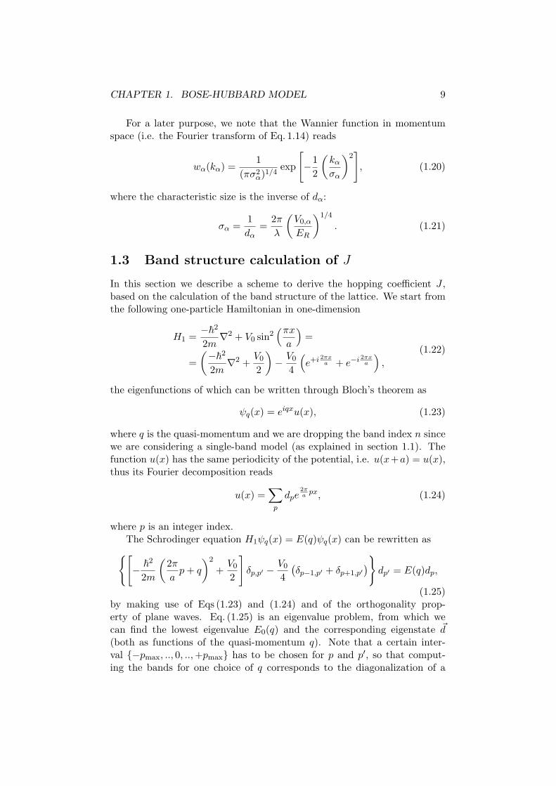
Figure 1.2: Band dispersion for different lattice depths s ≡ V0/ER, com-puted solving Eq. (1.25) for different values of qa and pmax = 5 (see text).
(2pmax + 1) × (2pmax + 1) matrix. Some examples of the band energy dis-persion En(q) are shown in Fig. 1.2; it can be noted that the single-bandapproximation is not a good assumption for very shallow lattice, in whichthe gap to the first band is smaller.
The energy spectrum is related to the hopping parameter JR betweentwo sites at distance Ra by the following relation [25]
∑
R
eiqaR = E0(q), (1.26)
where we are only considering the lowest energy level E0 on each site. IfEq. (1.26) is evaluated for a certain number D of values of q, this leads toa linear system of D equations in D variables that can be solved to find{J1, .., JD}. In our calculation we have chosen D = 6, after verifying thata larger value of D does not change the results for JR (with R ≤ 3). InTable 1.1 we show the results for the nearest-neighbour and next-nearest-neighbour coefficients J1 and J2, that are in agreement with the ones in Ref.[29]. We notice that J1 is always negative, meaning that there is a gain inenergy in nearest-neighbour hopping, whereas the next-nearest-neighbourhopping is not energetically favourable. Moreover, |J2| is always smallerthan |J1| and for realistic lattice depths the ratio |J2/J1| is lower than 1/10;

CHAPTER 1. BOSE-HUBBARD MODEL 11
Figure 1.3: Nearest neighbour hopping parameter (in semilog scale) asa function of the lattice depth. Results are obtained through Eq. (1.27)(dashed line) and band structure calculations (solid line).
in the same way, the values of JR are strongly suppressed for larger R. Thisis a justification for neglecting all the hopping processes with R ≥ 2.
V0/ER J1/ER J2/ER2 -0.14276 0.020394 -0.08549 0.006158 -0.03080 0.0006412 -0.01225 0.0000916 -0.00533 0.00001
Table 1.1: Nearest-neighbour and next-nearest-neighbour hopping coeffi-cients J1 and J2 for different lattice depths.
So far, we have only considered the energy dispersion and hopping pa-rameters for a one dimensional system. In the case of a separable lattice, thedimensionality does not affect the value of the hopping parameter; this isbecause we restrict our model to nearest-neighbour hopping processes, thathappen only along one of the possible directions. Thus one only needs toknow the value of J1 for the 1D model. On the contrary, for a non-separablelattice the hopping coefficients would have to be computed explicitly for thesystem with the correct dimensionality.
Considering the case of a separable isotropic lattice, an approximateexpression for the nearest-neighbour hopping coefficient J based on the so-lution of the Mathieu equation is given in Ref. [30]:
J
ER=
4√π
(
V0ER
)3/4
exp
(
−2
√
V0ER
)
. (1.27)

CHAPTER 1. BOSE-HUBBARD MODEL 12
In Figure 1.3 we compare the formula in Eq. (1.27) with the results of ourband-structure calculation.
1.4 Homogeneous phase diagram
It was first predicted by Matthew Fisher and collaborators in 1989 (Ref. [2])that the zero temperature phase diagram of the homogeneous Bose-Hubbardmodel
H = −J∑
〈i,j〉b†i bj +
U
2
∑
i
b†i b†i bibi − µ
∑
i
b†i bi, (1.28)
includes two different phases: a Mott-insulator phase in which a fixed (in-teger) number of particles are localized on every site and a superfluid phasein which particles are delocalized over a large region of the lattice. Here wedescribe the characteristic of the two phases and give some results for thephase diagram.
Large U/J : Mott insulating phase
If the repulsive on-site interaction is dominating (U/J ≥ 1) and the numberof particlesN is commensurate with the number of sitesNs, the ground stateof Eq. (1.28) is a Mott insulator. The extreme case is the one of vanishinghopping coefficient (J ≡ 0), that has the ideal Mott insulator state as anexact solution. This is the product of local Fock states with the same numbern0 (n0 ≡ N/Ns) of particles on every site
|ψMI〉 ≡ |ψMI〉J=0 ∝Ns∏
i=1
(
b†i
)n0
|0〉. (1.29)
This state has no occupation number fluctuations, all the sites host exactlyn0 particles. For a small but finite value of J/U , perturbation theory [31]leads to a state that is a dilute gas of particle/hole pairs immersed in a “sea”of sites with local density ni = n0
|ψMI〉J/U ≈ |ψMI〉+J
U
∑
〈i,j〉b†i bj |ψMI〉, (1.30)
where particle/hole excitations (also called doublon/holon) are only local-ized on neighbouring sites (up to first order in J/U).
Some features of the Mott state are: (a) the order parameter ψ ≡ 〈bi〉vanishes; (b) there is a gap in the excitation spectrum because the lowestexcitation is the creation of a particle-hole pair (corresponding to an energyof n0U); (c) the compressibility κ = ∂n
∂µ vanishes, i.e. the density remainsconstant as the chemical potential increases (in a certain range) and (d) thefluctuations of the number of particles per site are suppressed.

CHAPTER 1. BOSE-HUBBARD MODEL 13
Figure 1.4: Local occupation number distribution in the ideal superfluidstate (Eq. 1.31), for U/J = 0.
Small U/J : superfluid phase
If the kinetic term is dominating, the system reaches a superfluid phase, inwhich each single-particle state is delocalized over the lattice. For the idealcase of vanishing interaction (U/J = 0), the exact many-particle ground-state is
|ψSF〉 ∝(
b†k=0
)N|0〉 ∝
(
Ns∑
i=1
b†i
)N
|0〉. (1.31)
In this state, the local density distribution P (n) is a binomial distribution(see Ref. [32])
P (n) =e−N/Ns
n!
(
N
Ns
)n
. (1.32)
Some examples of this distribution are shown in Fig. 1.4, where it can benoticed that P (n) is not sharply peaked on a single local density n0. As acomparison, in the ideal Mott state (Eq. 1.29) we have P (n) = δn,n0
.The presence of local density fluctuations is one of the features of the
superfluid phase, not only in the ideal case of vanishing interactions. Otherfeatures include (a) the absence of an energy gap, (b) the finiteness of thecompressibility (this is seen in the monotonic increase of the density forincreasing chemical potential) and (c) the finiteness of the order parameter:|ψ| > 0.
Phase diagram
As we have described, the limit of weak interaction (strong interaction andcommensurate filling) corresponds to a superfluid (Mott insulator) phase.

CHAPTER 1. BOSE-HUBBARD MODEL 14
Figure 1.5: Left: phase diagram of the homogeneous one-dimensional Bose-Hubbard model (t corresponds to the hopping coefficient J); squares areQMC results (Ref. [33]), circles are DMRG results (Ref. [34]), the solidline is a strong-coupling expansion. Figure extracted from Ref. [35]. Right:boundaries of the first Mott lobe in the phase diagram of the homogeneoustwo-dimensional Bose-Hubbard model, obtained through QMC calculations.The inset shows a detailed view of the region of the tip. Figure adapted fromRef. [36].
Varying the ratio U/J or changing the chemical potential µ can lead to aphase transition.
In particular, we consider the (J/U)−(µ/U) phase diagram, that is char-acterized by some lobes (for low values of J/U) inside which the system is inthe Mott phase with an integer filling factor; outside these lobes, the systemis in the superfluid phase. The lines of fixed density do not correspond tolines of fixed chemical potential. In Fig. 1.5 we show accurate calculations ofthe first Mott lobe (i.e. the one with local density pinned to n0 = 1) in 1Dand 2D. They are qualitatively different, while the one in 3D is qualitativelythe same as in 2D. When the boundary of a lobe is crossed, a quantum phasetransition takes place. Depending on whether the crossing happens at fixeddensity or at fixed U/J , the transition has different universality properties[2].
In a site-decoupled mean-field approach (see section 3.2.2), the dimen-sionality of the system only enters the mean-field Hamiltonian through arescaling of J by the connectivity z, that is the number of nearest neigh-bours of each site (z = 2d for a d-dimensional hypercubic lattice). For thisreason, the mean-field (zJ/U) − (µ/U) phase diagram does not depend onthe dimensionality. In Fig. 1.6 we show the first Mott lobes computed bythis mean-field approach; by a comparison with Fig. 1.5 it can be notedthat the 1D mean-field phase diagram is qualitatively different from the realone, while in higher dimensions there is only a quantitative difference in theposition of the lobe tips.

CHAPTER 1. BOSE-HUBBARD MODEL 15
The phase diagram changes when other effects are taken into account.The inclusion of longer-range interactions is described in section 1.7 and hasbeen treated for instance in Refs [34, 8, 10]. The way in which the phasediagram changes for finite temperatures has been studied in Refs [37, 38, 39].
1.5 Inhomogeneous system: shell structure
As mentioned in section 1.1, in an experimental set-up the atoms are con-fined in space by a magnetic trap. In this section we describe the trappingpotential and the resulting shell structure in the local observables. Themain point here is that the trapping potential (i.e. the term
∑
i ǫini in thefull Hamiltonian Eq. 1.7) breaks the homogeneity of the system; thereforethere is not a single global phase of the system, but coexistence of differentphases is allowed. For the same reason, the superfluid-Mott insulator phasetransition is replaced by a phase crossover.
The trapping potential includes two different contributions: an externalmagnetic trap and the confinement due to the waist of the laser beams thatare used to create the optical lattice. For an optical lattice as in Eq. (1.4)and for a trapping potential as in Eq. (1.3), the frequency of the harmonictrap along the x direction is
ωTx =
√
ω2m +
4
m
(
V0,yw2y
+V0,zw2z
)
, (1.33)
where ωm is the frequency of the (isotropic) external magnetic trap and wy(wz) is the waist of the laser beam along the y (z) direction. Analogousrelations hold for ωTy and ωTz . In case of an isotropic lattice (with the samelattice depth V0 and the same beam waist w in every direction), the trappingfrequency reads [40]
ωT =
√
ω2m +
8V0mw2
. (1.34)
In Ref. [41], a correction to this expression has been proposed, to take intoaccount “the modification of the vibrational ground state energy in each welldue to the spatial variations of the laser intensities on the scale w”. Thecorrected expression for the isotropic case reads
ωT =
√
ω2m +
4(2V0 −√V0)
mw2. (1.35)
Independently from the strength of the trapping potential, its presencemakes it favourable an accumulation of the particles close to the center ofthe trap. When the local density in the center is larger than one, thereis a competition between the trapping potential and the repulsive on-site

CHAPTER 1. BOSE-HUBBARD MODEL 16
Figure 1.6: Left: mean-field phase diagram for the homogeneous system(solid lines), chemical potential in the center of the trap (cross mark), ef-fective local chemical potential in the trapped system (dashed vertical line).Right: radial dependence of the density (filled circles) and order parame-ter (crosses), obtained through the inhomogeneous site-decoupled mean-fieldapproach described in section 3.2.2.
interaction, since the latter favours a spread of the density over a largerregion. This competition leads to a shell structure for the density profile,meaning that along the radial direction the system is in a sequence of Mottand superfluid shells.
A first way of understanding this structure is the use of the Local DensityApproximation, based on the fact that the trapping potential changes slowlyon the typical system size. In this approximation, the trapping potential isincluded in an effective local chemical potential µi
µi = µ− ǫi, (1.36)
and for each site i the homogeneous system with chemical potential µi isstudied. In this approximation, the effective chemical potential in the centerof the trap corresponds to µ, while in all the other sites µi < µ and µidecreases with the distance from the center. If we put this set of effectivechemical potentials in the homogeneous phase diagram (see Fig. 1.6) we seethat for certain values of J/U this vertical line crosses different regions(corresponding to different phases).
This approximate explanation for the shell structure of the inhomoge-neous Bose-Hubbard model is confirmed by approaches that take into ac-count the inhomogeneity by studying the full Hamiltonian. In Figure 1.6an example is shown of the shell structure, computed through the inhomo-geneous mean-field approach described in Chapter 3. The formation of astructure including shells of different phases has been studied both numeri-cally (Refs [42, 43]) and in experiments (Ref. [44]).

CHAPTER 1. BOSE-HUBBARD MODEL 17
1.6 Time-of-flight measurements
One of the experimental techniques most frequently used to study a systemof cold atoms in an optical lattice is the measurement of the momentum dis-tribution via time-of-flight images. This is part of the following experimentalsequence
1. a Bose-Einstein condensate is prepared at low temperature (order of100− 102 nK), and a trapping potential is used to confine it in a finiteregion;
2. the laser beams needed to produce the optical lattice are slowly turnedon and their intensity is increased up to the required value of V0;
3. the system is kept on hold for a certain time interval;
4. all the potentials (the trapping potential and the lattice created bylaser beams) are suddenly turned off; the particles are now free andmove as plane-waves with a certain momentum k;
5. after a certain time interval τ , the particles are detected on a camerathrough absorption imaging of the atom cloud, leading to a map ofthe optical density distribution.
What is observed through this images is a density distribution in real spaceNtof(r). Assuming that when all the potentials are turned off the motion ofthe particle is free, this interference pattern in real space is interpreted as adistribution of momentum
Ntof(r)|k=mr
~τ=(m
~τ
)
|W (k)|2 S(k), (1.37)
where S(k) is defined as
S(k) ≡∑
i,j
eik·(ri−rj)〈b†i bj〉, (1.38)
and n(k) is the product of S(k) and the Wannier envelope
n(k) = |W (k)|2S(k). (1.39)
Some approximations are implied, when mapping the optical densityobserved in real space to the interference pattern n(k), as done in Eq. (1.37).This approach neglects the role of interaction during the expansion (after thetrap and lattice are turned off, the motion of particles is assumed to be free)and corrections due to the finiteness of the time interval τ . According to Ref.[45], these measurements are analogous to the observation of an interferencepattern in classical optics, in which a far-field condition is usually assumed.

CHAPTER 1. BOSE-HUBBARD MODEL 18
The corresponding far-field condition in case of time-of-flight measurementsis that τ should be much larger than a time-scale τff proportional to thecharacteristic coherence length. For a shallow lattice (i.e. for a small U/J)the coherence length is large and τff would be larger than the one typicallyused (see Ref. [45]).
We note that the difference between n(k) and S(k) is the Wannier en-velope |W (k)|2. Given the results derived in section 1.2, we are able toevaluate this envelope explicitely (in the harmonic approximation for thelattice wells) for any value of k.
Another feature of time-of-flight measurements is that only a 2D imageis detected in the experiments, rather than a map of the full 3D n(k). Whatis measured is n⊥(kx, ky), defined as the integral of n(k) along the probeline kz:
n⊥(kx, ky) =∫ +∞
−∞n(k)dkz =
∫ +∞
−∞|W (k)|2S(k)dkz. (1.40)
In the same way, S⊥(kx, ky) is defined as
S⊥(kx, ky) =n⊥(kx, ky)
|w1(kx)w2(ky)|2. (1.41)
The time-of-flight measurements that we have described have representedthe first experimental signature of the phase transition introduced in section1.4. In fact in the ideal superfluid phase there is a large phase coherenceand n(k) shows some sharp interference peaks, while in the Mott state thenumber of particles is fixed on every site and the phase fluctuates, leadingto a flat interference pattern (up to some small fluctuations).
In 2002, Markus Greiner and collaborators (Ref. [4]) performed this kindof measurements for different lattice depths. The results (Fig. 1.7) show thatfor increasing values of V0 (corresponding to increasing values of U/J) theinterference peaks smear out and only a uniform background remains. FromFig. 1.7 it can be also noted that what is observed is n(k) and not S(k), sincethe Wannier envelope suppresses the secondary peaks w.r.t. the central one.
1.7 Extended Bose-Hubbard model
For a system of atoms or molecules with a large dipole momentum, dipole-dipole long-range interactions are present in addition to the on-site repulsion(see Ref. [27] for an extended review). Here we consider the one-dimensionalextended Bose-Hubbard model for N bosons on a L-sites chain with periodicboundary conditions (PBC), described by the Hamiltonian
H = −tL∑
i=1
(
b†ibi+1 + b†i+1bi
)
+U
2
L∑
i=1
ni(ni − 1) + VL∑
i=1
nini+1, (1.42)

CHAPTER 1. BOSE-HUBBARD MODEL 19
Figure 1.7: Time-of-flight measurements of n⊥(kx, ky) for different latticedepths, from (a) to (h) V0/ER = 0, 3, 7, 10, 13, 14, 16, 20. Figure extractedfrom Ref. [4].
in which the term proportional to V corresponds to a repulsive interactionbetween bosons on neighbouring sites, due to dipole-dipole interactions.
Because of the presence of the long-range repulsion, the phase diagramincludes also a charge density wave (CDW) phase, in addition to the super-fluid and Mott insulator ones; this phase is characterized by periodic densityfluctuations around the average filling. In Ref. [34], this system was studiedin the gran-canonical ensemble (i.e. with a chemical potential µ to regulatethe number of particles) and it was shown how the phase diagram describedin section 1.4 changes to include lobes of CDW phase (Fig. 1.8).
More recently, in a series of work (Refs [8, 9, 10]) the extended Bose-Hubbard model in one dimension has been studied at unit filling and ithas been proposed that the long-range repulsion (either truncated to a dis-tance of one or three) can stabilize a fourth phase (the Haldane insulator),that is insulating but distinct from the Mott phase. In Fig. 1.9 the T = 0phase diagram is shown (for the case of repulsion truncated to the nearestneighbours).
In order to characterize the different phases of this system, we introducethe following set of correlation functions
CSF(r) = 〈b†j bj+r〉, (1.43)
CDW(r) = (−1)r〈δnjδnj+r〉, (1.44)
Cpar(r) =
⟨
exp
iπ
j+r−1∑
p=j
δnp
⟩
, (1.45)
Cstr(r) =
⟨
δnj exp
iπ
j+r−1∑
p=j
δnp
δnj+r
⟩
, (1.46)
where we have defined δnj ≡ (nj−1) and nj ≡ b†j bj . The first two correlators

CHAPTER 1. BOSE-HUBBARD MODEL 20
Figure 1.8: Phase diagram of the homogeneous one-dimensional Bose-Hubbard model with nearest-neighbour repulsive interaction(t ≡ J , U = 1,V = 0.4). The phases are: Mott insulator with filling one (MI), charge den-sity wave with filling one half (CDW) and superfluid (SF). Circles representDMRG results. Figure extracted from Ref. [34].
are local, i.e. they are of the form
C(r) = C(j, j + r) = 〈A(j)B(j + r)〉, (1.47)
whereas the parity and string correlation functions (Eqs 1.45 and 1.46) arenon-local, i.e. C(j, j + r) depends on all the sites between the sites j and(j + r).
The classification of the phases of the system is based on the infinite-distance limit of the correlation functions introduced in Eqs (1.43) - (1.46); inpractice most numerical methods deal with finite systems, thus the infinite-rlimit is replaced by the maximum distance rmax allowed on the lattice anda finite size scaling of the results is performed afterwards. The classificationof the phases based on the order parameters is the following [11]
phase CSF(∞) CDW(∞) Cpar(∞) Cstr(∞)
superfluid 6= 0 0 0 0Mott insulator 0 0 6= 0 0
Haldane insulator 0 0 0 6= 0density wave 0 6= 0 6= 0 6= 0
In Fig. 1.9 we show the phase diagram of this model obtained throughDMRG, from Ref. [10]. This is computed with a maximum occupationnumber of 3 bosons per site and using open boundary conditions (two op-

CHAPTER 1. BOSE-HUBBARD MODEL 21
Figure 1.9: Phase diagram of the extended Bose-Hubbard model (Eq. 1.42),from Ref. [10]. Energies in units of J .
posite biases have been added at the left and right boundaries of the chain,in order to lift the ground state degeneracy).

Chapter 2
Visibility in the trapped
system
As described in section 1.5, the presence of a trapping potential leads toa coexistence of different phases in the system. For very small values ofU/J (corresponding to a shallow lattice), the system is a single superfluiddomain; as U/J increases (corresponding to an increase of the lattice depthV0/ER), the Mott shells with integer filling appear.
In order to characterize the phase diagram of the system, there has beena large effort aimed at finding some experimentally measurable quantitiesthat can be used to probe the appearance of Mott domains. In many of theexperiments, time-of-flight images are taken, and the integrated interferencepattern n⊥(kx, ky) is measured. Different quantities can be extracted fromthese data: in some studies (Refs [4, 46]) the width of the interference peakhas been considered, while other authors have used the integral of the peak(Refs [47, 48]) or the peak weight (Ref. [49]).
Another way of characterizing the phase crossover is the visibility V ofthe interference pattern, that is a measure of the coherence of the system;this has been used for instance in Refs [31, 40, 50, 45, 51, 28].
In this chapter we first define and describe this quantity (section 2.1)and we review an experimental work (Ref. [31]) in which the visibility givessignatures of the appearance of Mott shells; this is linked to the presenceof non-smooth features (kinks) in the plot of V as a function of V0/ER.The results from Ref. [31] have been later compared with different numeri-cal simulations. QMC simulations of one-dimensional systems (reviewed insection 2.3) have been used to study the origin of the kinks. More recentQMC studies have achieved a quantitative description of the visibility bysimulating 2D or 3D systems of experimentally relevant sizes, but no kinkshave been observed; these studies are reviewed in section 2.4. In section 2.5we mention the presence of kinks in the visibility for another experimentalset-up, namely a triangular optical lattice (Ref. [28]).
22

CHAPTER 2. VISIBILITY IN THE TRAPPED SYSTEM 23
Figure 2.1: Position of kmax (filled circle) and kmin (empty circle); theshaded area corresponds to the first Brillouin zone.
2.1 Visibility
Given the definition of the integrated interference pattern n⊥(kx, ky) (Eq.1.40), we define its visibility V as in Ref. [31]:
V =n⊥(kmax)− n⊥(kmin)
n⊥(kmax) + n⊥(kmin), (2.1)
where
kmax =
(
2π
a, 0
)
, (2.2)
kmin =
(
2π
a√2,2π
a√2
)
, (2.3)
and where a is the lattice spacing. The definition of kmax and kmin is suchthat kmax is the center of one of the interference peaks of n⊥ (since this isthe center of the second Brillouin zone), while kmin is part of the incoherentbackground of n⊥. Therefore, the visibility is a contrast measurement be-tween the maximum and minimum values of n⊥. The reason for the specificchoice of kmin and kmax is that the Wannier functions in these two pointsare equal
|w1(kx)w2(ky)|2kmin= |w1(kx)w2(ky)|2kmax
, (2.4)

CHAPTER 2. VISIBILITY IN THE TRAPPED SYSTEM 24
because they are at the same distance from the origin (as shown in Fig. 2.1).Therefore, the Wannier envelope factorizes and cancels in Eq. (2.1) and thevisibility reads
V =(S⊥(kmax)− S⊥(kmin)) |w1(kx)w2(ky)|2kmax
(S⊥(kmax) + S⊥(kmin)) |w1(kx)w2(ky)|2kmax
=
=S⊥(kmax)− S⊥(kmin)
S⊥(kmax) + S⊥(kmin).
(2.5)
This quantity is a measure of the coherence of the system, useful to char-acterize its phase. In the superfluid phase there is coherence among particleson different sites and n⊥(kx, ky) shows sharp interference peaks; this leadsto a visibility close to unity (or identically one, for the homogeneous systemin the thermodynamic limit). On the contrary, for a homogeneous system inthe ideal Mott phase (J/U = 0) the local number of particles is fixed whilethe local phase is not; this leads to a homogeneous n⊥(kx, ky) distributionand to a vanishing visibility. In the trapped system there is not a singleglobal phase, thus the visibility can in principle take any intermediate valuebetween V = 0 and V = 1.
Moreover, the experimental results for the visibility V typically includealso other effects
• when extracting n⊥(kmax) and n⊥(kmin), these are averaged over acertain region around the specific points (e.g. in Ref. [31] this is aregion of 3× 3 pixels), to reduce the signal-to-noise ratio;
• n⊥(kmax) and n⊥(kmin) are averaged over the four copies of kmax andkmin obtained by rotations of π/2, π and 3π/2;
• these quantities are also averaged over different time-of-flight images,extracted from successive measurements.
2.2 First observation of kinks in VRefs [31, 40] are the first works in which the visibility of the quasimomentumdistribution is used to study the Mott-insulator transition of a bosonic gasin an optical lattice. The experimental set-up consists in a system of 87Rbatoms (scattering length as ≃ 5.45 nm) in a 3D optical lattice (laser wave-length λ = 850 nm, lattice spacing a = 425 nm, recoil energy ER ≈ h× 3.2KHz). The number of particles is of the order of 105 − 106, correspondingto approximately 3 particles per site in the center of the trap. The intensityof lattice potential is varied in the range V0/ER ∈ [5, 30].
The results for the visibility (Fig. 2.2) show the expected behaviour, i.e.V is close to unity for shallow lattices and it decreases for large values of V0.

CHAPTER 2. VISIBILITY IN THE TRAPPED SYSTEM 25
Figure 2.2: Visibility as a function of the lattice depth for a system of3.6×105 atoms (gray circles) and 5.9×10⁵ atoms (black circle). The seconddataset is vertically shifted for clarity. Figure adapted from Ref. [31].
In particular the behaviour for large V0 is in agreement with the estimate
V ∝ J
U, (2.6)
obtained perturbatively for the homogeneous system via a first order ex-pansion in terms of J/U (corresponding to the wave function in Eq. 1.30).Other details about the regime of deep lattice wells are given by the sameauthors in Ref. [40], in which a better estimate of the visibility is obtainedby computing it through the Green’s function within the Random-PhaseApproximation.
Another feature that can be observed in Fig. 2.2 is the presence of kinks inthe visibility, i.e. points in which the decay of V is not smooth; these can beeasily recognized by looking at the numerical derivative of the data. Thesekinks are “systematically observed” in “reproducible positions”, and theyappear at values of V0/ER close to the ones at which the Mott shells with n =2 or n = 3 particles per site are supposed to form. The explanation proposedby the authors is that “the observed kinks are linked to a redistribution inthe density as the superfluid shells transform into MI regions with severalatoms per site”.
2.3 Interpretation by QMC in 1D
After the experimental results described in the previous section were pub-lished, P. Sengupta and collaborators (Ref. [50]) proposed an explanation

CHAPTER 2. VISIBILITY IN THE TRAPPED SYSTEM 26
of the kinks in the visibility, based on a QMC study of the one dimensionalBose-Hubbard model in the trap 1.
The authors perform a study for fixed number of particles and describetwo different cases: in the first one the local occupation number does notreach two, so that only the Mott domain with n = 1 can form, whereas inthe second case also the Mott domain with n = 2 is present.
In the first case, for increasing U/J two kinks are observed in the (de-creasing) visibility: a less evident one at U/J = 6.3 and a second one aroundU/J = 7.1 (see Fig. 2.3(a)). The first kink is related to the emergence oftwo Mott plateaux on the sides of the central superfluid region, while thesecond one is related to the formation of a full Mott domain in the middleof the trap.
Figure 2.3: Left: 40 bosons on 80 sites, trapping potential VT(i) =(0.01 J)i2, less than two particles per site. (a) Visibility V and (maxS(k)),kinks at U/J ≃ 6.3 and 7.1. (b) Density profiles for different values of U/J(t corresponds to the hopping parameter J). Right: 60 bosons on 80 sites,trapping potential VT(i) = (0.06 J)i2. (c) Visibility V (d) Number of parti-cles Nc in the center of the trap, i.e. the sites i ∈ [−10, 10]. Figures adaptedfrom Ref. [50].
For intermediate values of U/J (i.e. between the two kinks), the densityprofile does not change (see Fig. 2.3(b)). This might seem in contrast withthe finite compressibility of the superfluid domain in the center of the trap,but the reason is that this domain is trapped between the Mott regions.Thus, particles can move from the center to the boundaries (where the
1In the previous section we have explained how the choice of the points kmin and kmax
matters in the definition of the visibility; in 1D the Brillouin zone is just the interval[−π
a, π
a] and there are no such points with the property of being at the same distance from
the origin. Moreover, in the theoretical works described in this section the system is trulyone-dimensional, thus no integration over kz is needed. Therefore, the visibility in 1D isdefined directly as in Eq. (2.5), by replacing S⊥(kmax) and S⊥(kmin) with the maximumand minimum of S(k).
CHAPTER 2. VISIBILITY IN THE TRAPPED SYSTEM 27
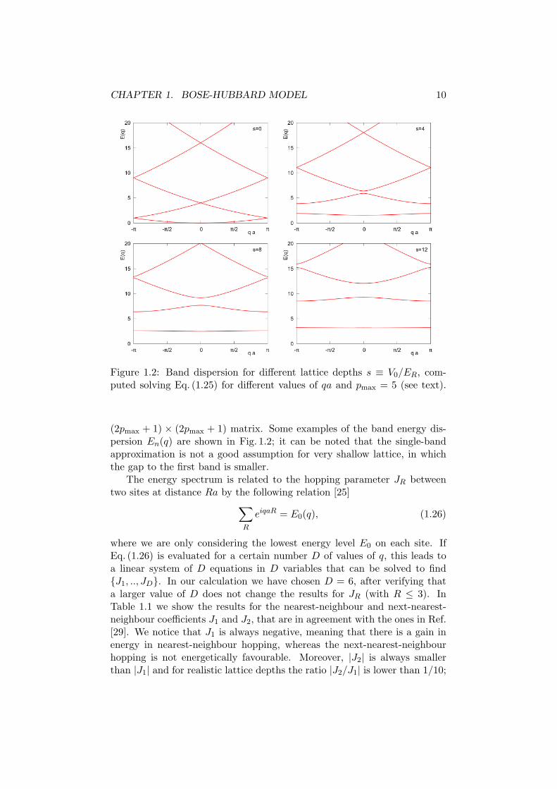
Figure 2.4: Canonical flows (i.e. lines with constant number of particles) inthe homogeneous phase diagram for the 1D system with VT (i) = 0.008 i2.Figure adapted from Ref. [52].
trapping energy is larger) only after U/J increases of a certain finite amount.In the range U/J = 6.3 − 6.8, also other quantities do not vary much (thetotal trapping energy, the interaction energy, the chemical potential).
In the simulation described in the second part of Ref. [50], also the Mottregion with two particles per site can form. Up to a certain value of U/J(U/J ∼ 13) the visibility has features similar to the previous case (see Fig.2.3(c)), while for larger values of U/J there are more kinks; these correspondto features in Nc (number of particle in the 20 central sites). These kinksdo not result from the formation of new Mott domains, but rather froma redistribution of bosons between the two existing Mott regions n = 2and n = 1. Such a redistribution happens discontinuously, leading to thefeatures in V. Moreover, the competition between the trapping potentialand the repulsive interaction is such that the size of the superfluid shoulderswith 1 < n < 2 is not always monotonously decreasing with U/J , and thiscan lead to an increase in V (e.g. the kink at U/t = 14.6).
Also a purely one-dimensional effect takes place, for larger values of U/J .When the Mott with n = 2 melts (i.e. there is a superfluid in the centerof the trap), correlations develop between the two disconnected superfluidshoulders with 1 < n < 2, and V increases. This would not happen in higherdimensionalities, since the superfluid region surrounding the center wouldbe a shell (or a ring, in 2D), and it would be already connected.
In Ref. [52], some of the same authors of Ref. [50] give more details toexplain the behaviour of the visibility. In particular, they map the canonicaltrajectories (i.e. the lines with fixed number of particles) on the homoge-neous phase diagram (as shown in Fig. 2.4) and they use this to interpretthe results for the visibility.
Following for instance the trajectory with N = 50 in Fig. 2.4 and com-

CHAPTER 2. VISIBILITY IN THE TRAPPED SYSTEM 28
Figure 2.5: Visibility in the 1D trapped system with VT (i) = 0.008 i2, for40 (squares) and 50 (triangles) particles. Figure adapted from Ref. [52].
paring it with the corresponding visibility (Fig. 2.5), it is clear that thesecond kink in the visibility V happens when the chemical potential in thecenter of the trap (i.e. µ, and not the effective local chemical potential µi)enters a Mott lobe. This corresponds to the closing of a Mott region in thecenter of the trap. On the other side, the position of the first kink in thevisibility is not directly read from the phase diagram. One would expect itsappearance for the first value of J/U lower than the tip of the Mott lobe(J/U < (J/U)c); however this happens for a smaller J/U . This means thatthe first kink does not correspond to the first appearance of the Mott re-gions, but rather to the value of U/J for which these regions gain a relevantsize.
2.4 Other QMC studies
The QMC studies described in the previous section are limited to one di-mension, thus they cannot achieve a quantitative agreement with results ofexperiments in 3D (Ref. [31]). In this section we review other QMC studies,more relevant for the direct comparison with experiments.
QMC in 2D
Ref. [53] is a QMC study in 1D and 2D, in which isentropical lines arefollowed, rather than lines at constant temperatures. The reason for this isthat what is constant during an experiment is the entropy, rather than thetemperature. The aim of this work is the study of the change of temperatureduring an experiment, also with the goal of verifying the typical assumptionsabout the adiabaticity of the lattice loading procedure.
The authors show the results (reported in Fig. 2.6) of a calculation
CHAPTER 2. VISIBILITY IN THE TRAPPED SYSTEM 29
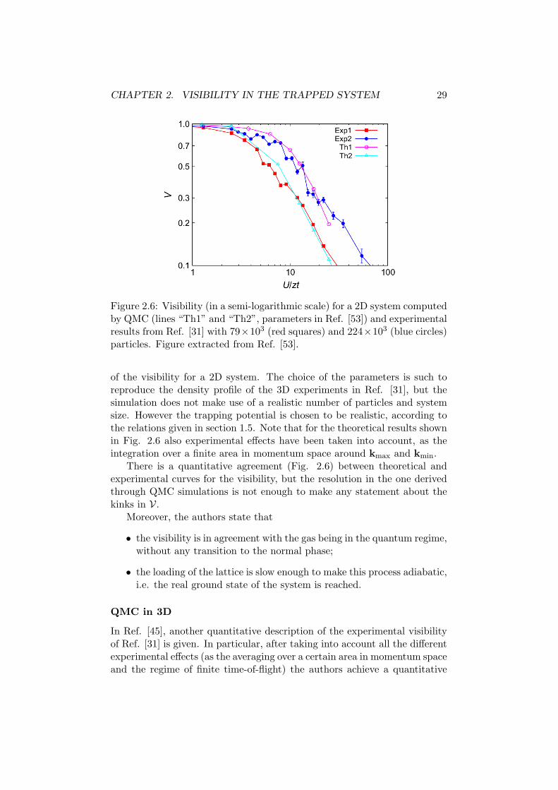
Figure 2.6: Visibility (in a semi-logarithmic scale) for a 2D system computedby QMC (lines “Th1” and “Th2”, parameters in Ref. [53]) and experimentalresults from Ref. [31] with 79×103 (red squares) and 224×103 (blue circles)particles. Figure extracted from Ref. [53].
of the visibility for a 2D system. The choice of the parameters is such toreproduce the density profile of the 3D experiments in Ref. [31], but thesimulation does not make use of a realistic number of particles and systemsize. However the trapping potential is chosen to be realistic, according tothe relations given in section 1.5. Note that for the theoretical results shownin Fig. 2.6 also experimental effects have been taken into account, as theintegration over a finite area in momentum space around kmax and kmin.
There is a quantitative agreement (Fig. 2.6) between theoretical andexperimental curves for the visibility, but the resolution in the one derivedthrough QMC simulations is not enough to make any statement about thekinks in V.
Moreover, the authors state that
• the visibility is in agreement with the gas being in the quantum regime,without any transition to the normal phase;
• the loading of the lattice is slow enough to make this process adiabatic,i.e. the real ground state of the system is reached.
QMC in 3D
In Ref. [45], another quantitative description of the experimental visibilityof Ref. [31] is given. In particular, after taking into account all the differentexperimental effects (as the averaging over a certain area in momentum spaceand the regime of finite time-of-flight) the authors achieve a quantitative

CHAPTER 2. VISIBILITY IN THE TRAPPED SYSTEM 30
Figure 2.7: The two upper lines are calculations for finite (dashed line) andinfinite (dotted-dashed line) time of flight, without considering experimentalresolution. The visibility for a 3D system (including the corrections for finiteexperimental resolution) are shown, as computed by QMC (solid line) andin experiments (Ref. [31], circles). Figure extracted from Ref. [45].
agreement of the experimental visibility with the curve obtained by QMCsimulations in 3D. This is shown in Fig. 2.7.
To conclude, in Ref. [53] and Ref. [45], a quantitative description of theexperimental visibility results from Ref. [31] is achieved; however, no kinksare observed in V. This could also be a by-product of the low resolution onthe U/J axis, in Figures 2.6 and 2.7.
2.5 Kinks in the triangular lattice
In Ref. [28] a different experimental set-up is presented, in which the opticallattice is a triangular one in two dimensions. This geometry is achieved by adifferent positioning of the laser beams and it is an example of the possibilityof describing different models with cold atoms in optical lattices.
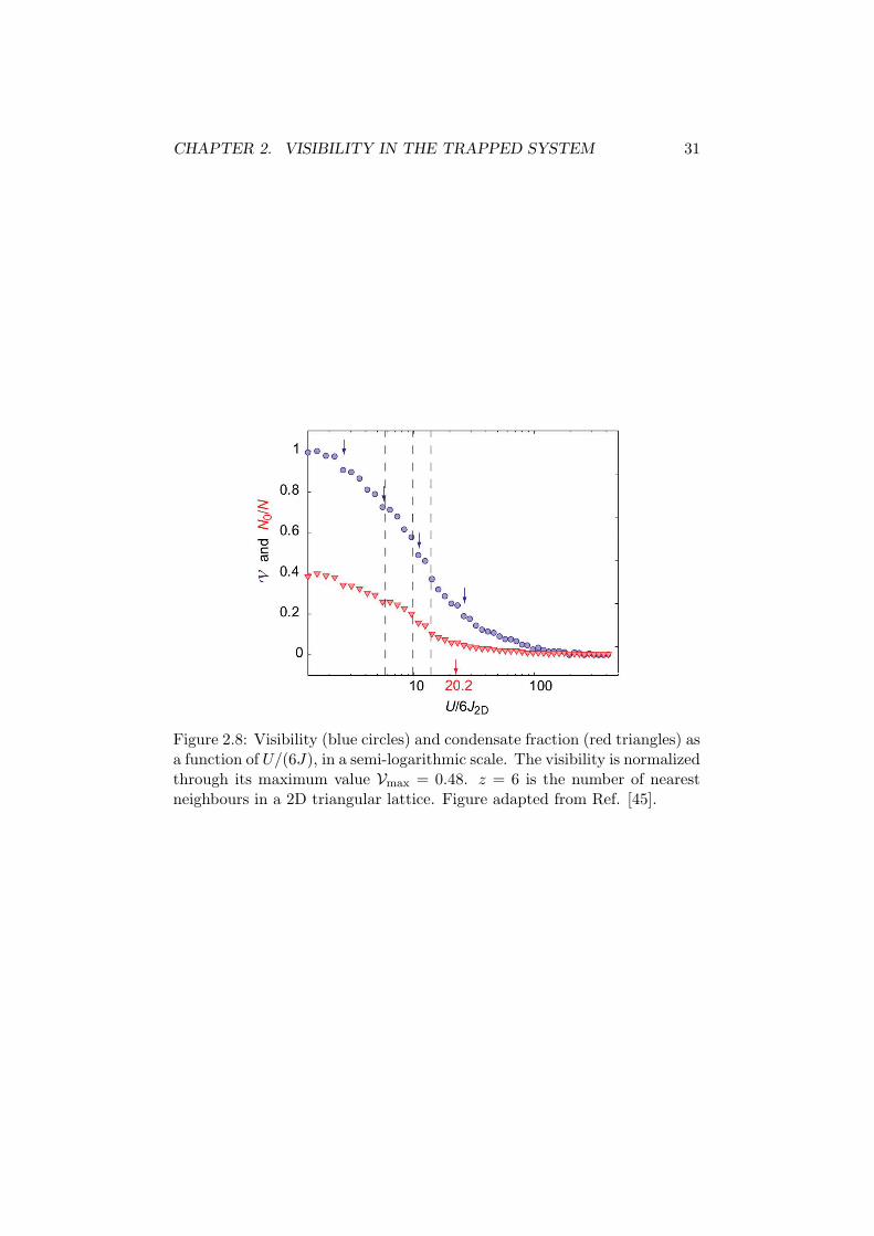
In Fig. 2.8, the visibility is shown for this system. Some kinks in Vare present, similar to the ones described in section 2.2. Unexpectedly, thepositions of these kinks are in close agreement with the positions of themean-field values of the critical coupling U/J (described in section 3.2).
Note that the number of nearest neighbours of a site in a triangularlattice is z = 6; this leads to a better agreement (as compared with thesquare lattice, where z = 4) of the mean-field results with the exact ones.
CHAPTER 2. VISIBILITY IN THE TRAPPED SYSTEM 31
Figure 2.8: Visibility (blue circles) and condensate fraction (red triangles) asa function of U/(6J), in a semi-logarithmic scale. The visibility is normalizedthrough its maximum value Vmax = 0.48. z = 6 is the number of nearestneighbours in a 2D triangular lattice. Figure adapted from Ref. [45].

Chapter 3
Numerical techniques
Since when fermionic Hubbard model and its bosonic equivalent were in-troduced, they have been often used as prototypical models to developand test new analytical and numerical solution techniques in the physicsof condensed-matter and many-body systems. For the bosonic model, thiseffort increased after its relation with cold-atomic systems was clarified, andit has been some times inspired from the study of the equivalent model forfermions.
In this chapter, we describe a few of the numerical schemes that canbe used to find the ground-state of the bosonic model and characterize itby evaluating correlation functions. As we mention at the end of this in-troduction, the list of techniques that have been developed is very large.We concentrate on the ones that we have used in this thesis, namely thesite-decoupled mean-field approach and the quantum Monte Carlo one.
In section 3.1 we describe the basic way of solving exactly any Hamilto-nian, and we explain why this approach cannot be used for large systems,that is linked to the exponentially growing dimension of the Hilbert space.A first solution of this problem is the decoupling of some terms in the Hamil-tonian, to reduce the complexity of the problem. The Bogoliubov approachdescribed in section 3.2.1 is based on the decoupling of the interaction term,but it does not describe correctly the Mott phase transition. On the contrary,the site-decoupled mean-field scheme described in section 3.2.2 is based onthe decoupling of the hopping term and succeeds in giving a description ofthe phase transition, although an approximate one. This method was firstproposed in Ref. [54] to study the homogeneous model and only recentlyit has been applied to the inhomogeneous one (Ref. [55]). It can be shownthat this approach is analogous to the use of the Gutzwiller variational wavefunction, that was first introduced to study the fermionic Hubbard modeland then adapted to the bosonic case (Refs [56, 3]). In section 3.2.3 wedescribe this ansatz and show its relation with the mean-field approach. Toconclude the description of the site-decoupled mean-field approach, in sec-
32

CHAPTER 3. NUMERICAL TECHNIQUES 33
tion 3.2.4 we explain some details on how to implement the it numericallyand in section 3.3 we compare its results with some known ones. In Section3.4 we describe two QMC approaches: the variational Monte Carlo (VMC)scheme and the Green’s Function Monte Carlo (GFMC) scheme. The resultsof the latter do not depend on initial assumptions about the ground-stateand are in principle unbiased (for bosonic problems).
In general, the numerical techniques applied to study the Bose-Hubbardmodel (and the analogous models with a trapping potential, long-range in-teractions, disorder, or finite temperature) have included a large set of ap-proaches. As a partial list, we mention some works based on the maintechniques
• Gutzwiller wave function and corresponding mean-field theory (for ho-mogeneous and trapped systems), Refs [56, 54, 57, 58, 59, 60, 61, 55];
• cluster mean-field theory, Refs [62, 63, 64];
• a large set of different QMC schemes (including VMC, GFMC, PathIntegral Monte Carlo, Strong Series Expansion), Refs [65, 66, 50, 37,67, 52, 36, 68, 53, 49, 69, 14, 11];
• DMRG (introduced in Ref. [16]), Refs [34, 70, 71, 8, 9, 72, 10];
• Matrix Product States, Ref. [12];
• Dynamical Mean Field Theory for bosons, Refs [73, 74, 75];
• exact diagonalization schemes, Refs [76, 3, 77].
3.1 Exact diagonalization
In this section we describe an exact diagonalization (ED) scheme to ob-tain the full spectrum and eigenstates of the Hamiltonian. We stress thatanother ED scheme exists (the one based on the Lanczos algorithm, not de-scribed here), that targets only the lowest eigenvalues and the correspondingeigenstates of the Hamiltonian. Since this method requires less CPU timeand memory, it allows to study larger systems and it would be the mostappropriate choice for a study only based on ED. We do not consider it herebecause we will use ED only as a benchmark for other methods.
The general procedure for diagonalizing the full Hamiltonian is the fol-lowing
• choose a basis {|φj〉}j=1,..,D of the Hilbert space of the system and listits D states;
• construct the D ×D matrix representation of the Hamiltonian in thechosen basis, according to Hi,j = 〈φi|H|φj〉;

CHAPTER 3. NUMERICAL TECHNIQUES 34
• diagonalize the matrix Hi,j , in order to get the full set of eigenvaluesand eigenvectors {Ej , ~vj}j=1,..,D.
At the end of this procedure, the lowest eigenvalue is identified with theground state energy and the corresponding eigenvector is the ground statewave function in the basis {|φj〉}j=1,..,D
Egs = minj
(Ej), (3.1)
H~vgs = Egs~vgs. (3.2)
and any observable expressed as an expectation value on the ground state|ψ0〉 can be computed as
〈ψ0|A|ψ0〉 =D∑
j=1
|vjgs|2〈φj |A|φj〉. (3.3)
In the case of a system of N bosons on a lattice of L sites, we choose theoccupation numbers basis
|x〉 = |n1, n2, ..., nL〉 ≡ |n1〉1 ⊗ |n2〉2 ⊗ ..⊗ |nL〉L. (3.4)
The number D of terms in the basis (i.e. the dimension of the Hilbert space)grows as
D =
(
N + L− 1
L− 1
)
=(N + L− 1)!
N !(L− 1)!. (3.5)
As an example, in Table 3.1 we show the number of states at unit filling(N = L) for some system sizes:
N D N D
4 35 10 923786 462 20 689232644108 6435 30 59132290782430712
Table 3.1: Number of states for a system of N indistinguishable bosons inN sites.
This makes it clear that the full ED approach can only work for smallsystems.
Notice that in the matrix representation of H many entries are zero (allthe ones corresponding to two different states not connected through a hop-ping process). Nevertheless, also the Lanczos algorithm will face the problemof the exponential growth of D, making the study of large system impossi-ble. For this reason, we will not use ED to study the physical properties ofthe system in the thermodynamic limit (N,L→ ∞, N/L = const), but onlyas a benchmark for other methods. Notice that ED finds applications alsoas a part of more complex methods, like Numerical Renormalization Groupand Dynamical Mean Field Theory.

CHAPTER 3. NUMERICAL TECHNIQUES 35
3.2 Mean-field approaches
We present here some mean-field approaches for the homogeneous and inho-mogeneous Bose-Hubbard models introduced in Eqs (1.7) and (1.28). Thefirst approach that we describe is the Bogoliubov approximation (for thehomogeneous system), that is based on the decoupling of the interactionterm; this technique is not able to correctly describe the Mott phase transi-tion. In section 3.2.2 we describe another mean-field scheme, based on thedecoupling of the hopping term in the Hamiltonian. This approach succeedsin predicting the Mott phase transition, although in an approximate way.It has been shown later that using this mean-field approach corresponds toa variational calculation based Gutzwiller ansatz. This link is described insection 3.2.3 and it explains why this approach is more suitable (as comparedto ED) to study large systems. More concretely, in sections 3.2.4 and 3.3we describe the numerical scheme we used and we validate it by comparisonwith known results in the literature.
3.2.1 Bogoliubov approximation
The Bogoliubov transformation is a general method that allows to diagonal-ize some Hamiltonians, the most common example being in the context ofthe BCS theory of superconductivity. In this section (mainly based on Ref.[57]), we consider the homogeneous Bose-Hubbard model on a d-dimensional
hypercubic lattice with spacing a. By introducing the operators c†k and ckthrough
bi =1√Ns
∑
k
cke−ik·xi (3.6)
(where Ns is the total number of sites), the Hamiltonian can be written inmomentum space as
H =∑
k
(−ǫk − µ)c†kck +1
2
U
Ns
∑
k,k′
∑
k′′,k′′′
c†kc†k′ ck′′ ck′′′δk+k′δk′′+k′′′ , (3.7)
where ǫk = 2J∑d
j=1 cos(kja) is the dispersion related to the kinetic term.We note here that for U = 0 this Hamiltonian is diagonal and its ground-state is the one with N bosons in the k = 0 minimum of ǫk:
(
c†k=0
)N|0〉, (3.8)
corresponding to the ideal superfluid state introduced in Eq. (1.31).
Assuming that the number of condensate atoms N0 = 〈c†0c0〉 is muchlarger than unity (assumption valid in the weakly interacting limit) and
choosing the expectation values of c†0 and c0 to be real, the Bogoliubov

CHAPTER 3. NUMERICAL TECHNIQUES 36
approach consists in replacing these operators with their average plus afluctuation (that we call with the same names)
c0 →√
N0 + c0,
c†0 →√
N0 + c†0.(3.9)
Substituting Eq. (3.9) into Eq. (3.7) and setting to zero the part of the
Hamiltonian that is linear in the fluctuation terms c†0 and c0, we find thecondition
µ = UN0/Ns − zJ (3.10)
(in which z = 2d is the number of nearest neighbours of a site) and thefollowing effective Hamiltonian
Heff =− 1
2Un0N0 −
1
2
∑
k
(ǫk + Un0)+
+1
2
∑
k
(c†k, c−k)
[
ǫk + Un0 Un0Un0 ǫk + Un0
](
ckc†−k
)
,
(3.11)
in which we have introduced ǫk = zJ − ǫk and n0 = N0/Ns and we havekept only terms up to second order in the fluctuations. This Hamiltonian isdiagonalized by means of the substitution
(
dkd†−k
)
=
[
uk vkv∗k u∗k
](
ckc†−k
)
, (3.12)
in which the condition |uk|2−|vk|2 = 1 is required so that the new operators
d†k and dk satisfy the bosonic commutation relations. This leads to thediagonal Hamiltonian
Heff = −1
2Un0N0 +
1
2
∑
k
[~ωk − (ǫk + Un0)] +∑
k
~ωkd†kdk, (3.13)
with the dispersion relation
~ωk =√
ǫ2k + 2Un0ǫk, (3.14)
and the following values of the coefficients
|vk|2 = |uk|2 − 1 =1
2
(
ǫk + Un0~ωk
− 1
)
. (3.15)
CHAPTER 3. NUMERICAL TECHNIQUES 37
For this effective Hamiltonian, the total density is given by the sum of thecondensate density n0 and the density due to the excitations
n =1
Ns
∑
k
〈c†kck〉eff =
= n0 +1
Ns
∑
k 6=0
[
(|uk|2 + |vk|2)〈d†kdk〉eff + |vk|2]
=
= n0 +1
Ns
∑
k 6=0
[
(|uk|2 + |vk|2)1
eβ~ωk − 1+ |vk|2
]
,
(3.16)
where 〈..〉eff denote the expectation value calculated with the effective Hamil-tonian Heff . In the limit of zero temperature the first term in the summandvanishes and the following relation can be obtained in the continuum limit
n = n0 +1
2
+1/2∫
−1/2
dq
(
ǫq + Un0~ωq
− 1
)
, (3.17)
with ǫq =∑d
j=1[1− cos(2πqj)] and ~ωq = (ǫ2q + 2Un0ǫq)1/2.
Eq. (3.17) has been used in Ref. [57] to compute the condensate fractionn0/n for different filling factors n and for different values of U/J . Numer-ical results for integer and non-integer filling factor do not show relevantdifferences and in both cases there is no critical value of U/J above whichthe condensate fraction vanishes. This is a sign of the fact that Bogoliubovapproximation does not predict the phase transition to the Mott insulatorphase, the reason being that the approximated treatment of interactionscannot be used when describing a strongly depleted condensate. Neverthe-less, this approach turns out useful in the regime of weak interactions, whereit is mostly effective to compute observables that are defined in momentumspace.
3.2.2 Site-decoupled mean-field approach
In this section we describe a mean-field approach based on the decouplingof the hopping part of the Hamiltonian, introduced by K. Sheshadri andcollaborators in 1993 (Ref. [54]). Considering the inhomogeneous Bose-Hubbard Hamiltonian (Eq. 1.7), we use the following decoupling
b†i bj = 〈b†i 〉bj + b†i 〈bj〉 − 〈b†i 〉〈bj〉 = ψibj + ψj b†i − ψiψj , (3.18)
where we have introduced the real order parameter ψi ≡ 〈bi〉. Note that thechoice of ψi ∈ R is arbitrary, but it is justified by the fact that the phaseof ψi does not enter explicitly in the procedure for finding the ground-state.

CHAPTER 3. NUMERICAL TECHNIQUES 38
By using Eq. (3.18), the Hamiltonian becomes a sum of local terms
H =∑
i
HMFi (ψi, {ψj}nni), (3.19)
where the local mean-field Hamiltonian HMFi on the site i depends on the
other sites only through the order parameters ψj on the sites j that arenearest neighbours of i (i.e. j ∈ nni). The explicit expression is
HMFi = J
∑
j∈nniψj
(
ψi − b†i − bi
)
+
(
U
2ni(ni − 1) + (ǫi − µ)ni
)
. (3.20)
We will now describe the difference between the homogeneous (ǫi = 0)and inhomogeneous (ǫi 6= 0) cases. In the homogeneous case, the observ-ables are not site-dependent and in particular ψi = ψ. Therefore the localHamiltonians are completely decoupled and equivalent, and each one of themreads
HMF(ψ) = Jzψ(
ψ − b† − b)
+
[
U
2n(n− 1)− µn
]
. (3.21)
This can be expressed as a tridiagonal matrix in the occupation numberbasis {|n〉}:
〈p|HMF|q〉 =[
zJ |ψ|2 − qµ+U
2q(q − 1)
]
δq,p−zJψ√pδq,p−1−zJψ
√qδp,q−1.
(3.22)A maximum number nmax of bosons per site has to be chosen; as an example,the matrix representation with nmax = 4 is:
zJ |ψ|2 −zJψ 0 0 0
−zJψ zJ |ψ|2 − µ −√2zJψ 0 0
0 −√2zJψ zJ |ψ|2 − 2µ+ U −
√3zJψ 0
0 0 −√3zJψ zJ |ψ|2 − 3µ+ 3U −2zJψ
0 0 0 −2zJψ zJ |ψ|2 − 4µ+ 6U
.
(3.23)In the inhomogeneous case (not treated in Ref. [54], but recently de-
scribed in Ref. [55]) the order parameter depends on the site index, andtherefore also the matrix in Eq. (3.23) does. Hence, the local Hamiltoni-ans HMF
i (ψi, {ψj}nni) are no longer decoupled (because the hopping termdepends on the values of the order parameter in the neighbouring sites)and all of them have to be diagonalized simultaneously. In section 3.2.4 wedescribe a self-consistent approach that allows us to do so.
3.2.3 Gutzwiller ansatz
The Gutzwiller wave function is a variational ansatz that was first introducedto study the fermionic Hubbard model. It has then been applied also in

CHAPTER 3. NUMERICAL TECHNIQUES 39
the context of the bosonic model (Refs [78, 56]), in which it has also beenmodified to a different version, that is the one we are presenting here. Thevariational ansatz is the following product of independent states on everysite
|ψg〉 =Ns∏
i=1
[ ∞∑
ni=0
f (i)ni|ni〉]
, (3.24)
where the coefficients f(i)ni are to be optimized in the variational procedure.
This choice of the wave function restricts the dimensionality D of the Hilbertspace to
D = Ns × (nmax + 1), (3.25)
where nmax is the already mentioned maximum on-site occupation number.This quantity (D) increases only linearly with the system size (to be com-pared with the exponential growth in Eq. 3.5), thus making it possible tostudy larger system, as compared to the ones that can be studied by EDmethods. The drawback is that the Gutzwiller wave function includes nocorrelations between different sites; this approximation is particularly poorin the description of the Mott state, since the state at finite J is replacedwith the ideal state (correct only for J/U ≡ 0). This problem will be thereason for a lack of agreement with QMC results in some specific cases (seesection 3.3).
Using this ansatz, the following expectation values can be computed in
terms of the coefficients{
f(i)ni
}
:
ρij ≡ 〈b†i bj〉g =( ∞∑
ni=0
f(i)∗ni+1f
(i)ni
√ni + 1
)
∞∑
nj=0
f (j)∗njf(j)nj+1
√
nj + 1
,
(3.26)
〈b†i bi〉g =∞∑
ni=0
∣
∣
∣f (i)ni
∣
∣
∣
2ni, (3.27)
〈b†i b†i bibi〉g =
∞∑
ni=0
∣
∣
∣f (i)ni
∣
∣
∣
2ni(ni − 1), (3.28)
〈bi〉g =∞∑
ni=0
f (i)∗nif(i)ni+1
√ni + 1. (3.29)
From these results, we can compute the expectation value of the Bose-

CHAPTER 3. NUMERICAL TECHNIQUES 40
Hubbard Hamiltonian (Eq. 1.7) on the state |ψg〉:
〈H〉g =− J∑
〈i,j〉
( ∞∑
ni=0
f(i)∗ni+1f
(i)ni
√ni + 1
)
∞∑
nj=0
f (j)∗njf(j)nj+1
√
nj + 1
+
+U
2
Ns∑
i=1
∞∑
ni=0
∣
∣
∣f (i)ni
∣
∣
∣
2ni(ni − 1) +
Ns∑
i=1
(ǫi − µ)∞∑
ni=0
∣
∣
∣f (i)ni
∣
∣
∣
2ni.
(3.30)As we did for the site-decoupled mean-field approach, we stress the differ-
ence in the application of this scheme to the homogeneous or inhomogeneousHamiltonian. In the homogeneous case (ǫi = 0), the coefficients fn are notfunction of the site index; thus Eq. (3.30) becomes
〈H〉gNs
=
[
−zJ∞∑
n=1
∞∑
m=1
f∗nfn−1f∗m−1fm
√nm+
∞∑
n=0
|fn|2(
U
2n(n− 1)− µn
)
]
.
(3.31)In order to describe the ground state of the system, the coefficients in theGutzwiller state have to be the ones that minimize this expectation value.This is a function of (nmax+1) variables; for typical values of nmax, the min-imization can easily be performed numerically. Once the fn coefficients areknown, observables can be computed through Eqs (3.26)-(3.29) and analo-gous expressions.
In principle the same approach can be used also in the inhomogeneouscase, but it has to be applied to the full Hamiltonian (Eq. 3.30); thus theminimization involves (nmax + 1)×Ns variables, while in the homogeneouscase these are only (nmax + 1). As an example, the number of variables fora 5× 5× 5 lattice with a cut-off nmax = 4 is 5 in the homogeneous case and625 in the inhomogeneous one. Note that the symmetries of the trappingpotential can be used to reduce this number in the inhomogeneous case. Forinstance, we have typically restricted our calculations to the sites (i, j, k)with i, j, k ≥ 0, making use of the symmetry of VT (x) under rotations todescribe the rest of the lattice.
Link with the mean-field approach
When the total Hamiltonian of the system is written as a sum of local termsas in Eq. (3.19), the Gutzwiller ansatz (Eq. 3.24) is the most general form
of the eigenstates. Hence, the coefficients ~f i = {f (i)n } correspond to theeigenvectors of the mean-field local Hamiltonian matrix (Eq. 3.22) and thesite-decoupled mean-field approach is equivalent to the minimization basedon the Gutzwiller ansatz. Therefore the two methods (the diagonalizationof the mean-field Hamiltonian and the minimization of the Gutzwiller en-ergy) are equivalent. We choose to use the diagonalization of the mean-field
CHAPTER 3. NUMERICAL TECHNIQUES 41
Hamiltonian in order to avoid the task of minimizing functions of manyvariables, and we use the Gutzwiller coefficients to compute expectationvalues.
3.2.4 Numerical scheme
In this section we explain more in detail the possible schemes to use themean-field/Gutzwiller approach that we have described.
Homogeneous case
The study of the homogeneous system does not involve large calculations,for the reasons explained before. In any case different schemes can be used:
1. one choice is that of considering the Hamiltonian in Eq. (3.22), findingits (nmax+1) eigenvalues Eα(ψ) analytically and minimizing the lowestone w.r.t. the order parameter ψ. This corresponds to finding
minψ
minα∈{0,..,nmax}
Eα(ψ). (3.32)
2. a second possible choice is that of using a self-consistent loop. TheHamiltonianHMF is diagonalized for a certain value of ψ, after which anew value ψnew of the order parameter is computed by Eq. (3.29). If thetwo quantities are not equal (up to a certain numerical tolerance), ψ isconveniently changed and the procedure is repeated till convergence.
Inhomogeneous case
Also in the inhomogeneous case the same two schemes (conveniently gener-alized from a single site to the full lattice) can be used. Both methods canbe applied when the chemical potential µ is fixed (i.e. only the Gutzwillercoefficients {~f i} are unknown) or when the number of particles is fixed (i.e.also the chemical potential is unknown).
We begin by considering the case of fixed chemical potential. The mini-mization procedure is performed in the following way
• diagonalize the local Hamiltonian in the truncated basis on each site(this is a (nmax + 1) × (nmax + 1) matrix that is real, symmetric andtridiagonal);
• identify the lowest eigenvalue Eg({ψi}) of the total Hamiltonian (sumof all the local ones);
• minimize Eg with respect to {ψi};
• compute local observables through the Gutzwiller coefficients {~f i}.

CHAPTER 3. NUMERICAL TECHNIQUES 42
The self-consistent loop approach is the following
• initialize the set of values of the order parameter on the entire lattice{ψi}old;
• diagonalize the local Hamiltonian in the truncated basis on each site;
• compute the new order parameters {ψi}new, through the Gutzwillercoefficients (Eq. 3.29);
• compare {ψi}old and {ψi}new by evaluating the norm of their differencein R
Ns
– if they differ more than a certain chosen tolerance, update theorder parameters with the new values and repeat the diagonal-ization;
– if they are close enough, keep the new values of the order pa-rameters and Gutzwiller coefficients and use them to computeobservables.
The scheme to work at a fixed number of particles (valid for both meth-ods) is the following
• initialize the chemical potential µ;• perform either the minimization or the self-consistent loop;• compute the number of particles N through the Gutzwiller coefficients(Eq. 3.27);
• compare N and N : if they differ less than a certain tolerance then thecalculation stops, otherwise µ has to be modified and the previous twosteps have to be repeated until convergence.
In particular, we use the secant method to decide how to modify µ in orderto make |N −N | decrease and vanish.
As we discussed before, in the inhomogeneous case the minimizationinvolves a large number of variables. For this reason, we have used theminimization approach only in the homogeneous case, to validate the resultsof the self-consistent approach. In section 3.3.1 we report a comparison ofthe two methods for the homogeneous system, while for the inhomogeneouscase we have only used the self-consistent approach.
3.3 Validation of the mean-field scheme
In this section we show the results of some calculations used to test andvalidate the mean-field approach. In particular, in section 3.3.1 we comparethe two methods described in section 3.2.4; in section 3.3.1 we study thevisibility of the homogeneous system and compare the results with the ones

CHAPTER 3. NUMERICAL TECHNIQUES 43
Figure 3.1: Left: Mean-field calculation of the density n and the condensatedensity n0 ≡ |ψ|2 as functions of the chemical potential µ, for a fixed valueof U = 12zJ and with nmax = 5. The results for n0 are obtained through theself-consistent loop scheme (solid line) and through the minimization scheme(points); the difference between the two is hardly visible. Right: (a) phasediagram and (b) density along the line with U = 12 (energies expressed inunits of zJ). Figure extracted from Ref. [54].
from Ref. [79]; in section 3.3.2 we show that our results are in qualitativeagreement with mean-field calculation from Refs [58, 59], which comparewell with QMC results from Ref. [65].
3.3.1 Homogeneous system
Self-consistent loop vs minimization
In section 3.2.4 we described two methods to find the ground state of themean-field Hamiltonian, namely a minimization w.r.t. the order parame-ter ψ and the scheme based on the self-consistent loop. In Fig. 3.1 weshow the results for the density n and condensate density n0 as functionsof the chemical potential; we set U = 12zJ , in order to compare the resultswith those in Ref. [54]. As expected, we observe the presence of the Mottphase characterized by integer filling, incompressibility (vanishing derivativeof n = n(µ)) and vanishing condensate density. The condensate density iscomputed with the two methods described in 3.2.4 and the difference be-tween the results is hardly visible in the plot. The density as a function ofµ is in agreement with results in Ref. [54], also shown in Fig. 3.1.
Calculations of visibility
In this section we compare results obtained in different ways for the visibilityof a 3D homogeneous Bose-Hubbard model, in a region of the phase diagram

CHAPTER 3. NUMERICAL TECHNIQUES 44
close to the tip or the Mott lobe with filling one. This point is
(
U
zJ
)
c
≃ 5.83,
( µ
zJ
)
c≃ 0.4
(
U
zJ
)
c
= 2.33,
(3.33)
as given in Refs [80, 57].Our goal is to compare the visibility of the interference pattern computed
in two different ways:
• the standard definition introduced in section 2.1 (see Refs [65, 45]),that remains valid also in the inhomogeneous case;
• the expression (specific for the homogeneous case) derived in Ref. [79].
In both approaches, the finiteness of the system has an effect on n(k) andthen on the visibility; for this reason we have repeated the calculations fordifferent lattice sizes and compared the results.
Here we repeat some of the steps used in Ref. [79] to derive an expressionfor the visibility. From the mean-field decoupling (Eq. 3.18), we have that
〈b†i bj〉 ={
|ψ|2 (i 6=j)n (i=j)
, (3.34)
and this leads to the following rewriting of S(k) (defined in Eq. 1.38):
S(k) =∑
i
n+∑
i
eik·ri∑
j 6=ie−ik·rj |ψ2| = N + |ψ2|
∑
i
eik·ri
−e−ik·ri +∑
j
e−ik·rj
=
= N + |ψ2|∑
i
eik·ri∑
j
e−ik·rj − |ψ|2∑
i
1 = (N −N0) + |ψ|2∣
∣
∣
∣
∣
∑
i
eik·ri
∣
∣
∣
∣
∣
2
≡
≡ (N −N0) + |ψ|2f(k),(3.35)
where N (N0) is the number of particles (condensed particles). We haveintroduced
f(k) =
∣
∣
∣
∣
∣
∑
i
eik·ri
∣
∣
∣
∣
∣
2
=3∏
j=1
∣
∣
∣
∣
∣
∣
L∑
j=1
eikjja
∣
∣
∣
∣
∣
∣
2
=3∏
j=1
F (kj), (3.36)
where a is the lattice spacing; for cubic L× L× L lattice, F (k) reads
F (k) =
(
sin(kLa/2)
sin(ka/2)
)2
, (3.37)

CHAPTER 3. NUMERICAL TECHNIQUES 45
and it satisfies:F (0) = L2,
F (2π/a) = L2,
F (√2π/(2a)) ≪ L2.
(3.38)
We now make use of the Gaussian form of the Wannier functions (approxi-mation introduced in section 1.2), in which σ is the characteristic spread ofthe Gaussian in momentum space. Thus the visibility defined in Eq. (2.1)can be rewritten as
V =n⊥(2π/a, 0)− n⊥(2π/(
√2a), 2π/(
√2a))
n⊥(2π/a, 0) + n⊥(2π/(√2a), 2π/(
√2a))
=
=|ψ|2
[
F (0)F(
2πa
)
− F(√
2π2a
)
F(√
2π2a
)]
∫
dqzF (qz)|w(qz)|2
2(N −N0) + |ψ|2[
F (0)F(
2πa
)
+ F(√
2π2a
)
F(√
2π2d
)]
∫
dqzF (qz)|w(qz)|2≃
≃ |ψ|2L4∫
dqzF (qz)|w(qz)|22(N −N0) + |ψ|2L4
∫
dqzF (qz)|w(qz)|2=
|ψ|2|ψ|2 + (N −N0)y
,
(3.39)where y is introduced as
y =2
L4
1∫
dqz|w(qz)|2F (qz)(3.40)
and it is approximated as
y ≈ σa
L5√π. (3.41)
In Fig. 3.2, we show the visibility computed by the standard definitionand by Eq. (3.39), for different lattice sizes. There is a good agreementbetween the different results, that are both based on the same mean-fielddecoupling. Note that Eq. (3.39) includes an approximation for y (Eq. 3.41).
We stress that the size of the system does not play any role in determin-ing the ground-state (i.e. the Gutzwiller coefficients), but it matters in thecomputation of the Fourier transforms required in the momentum distribu-tion. In the thermodynamic limit, the peaks in the momentum distributionwould be very sharp (δ-like) in the superfluid phase, while in the Mott phasen(k) would be completely flat. Therefore the visibility would have a sharptransition between V = 1 (superfluid phase) and V = 0 (Mott phase). Asshown in Fig. 3.2, results obtained with both approaches change in thecorrect way for increasing system size.
3.3.2 Inhomogeneous system
In Refs [58, 59, 60], the results of mean-field calculations in the 3D trappedcase are shown and compared with the same results computed by QMC(Ref. [65]). The quantities that are computed include the density profiles

CHAPTER 3. NUMERICAL TECHNIQUES 46
Figure 3.2: Visibility of a L × L × L homogeneous system computed usingthe standard definition in Eq. (2.1) (crosses) and the expression in Eq. (3.39)from Ref. [79] (open circles). The expected mean-field critical value of U/zJis also shown (dashed line).
and the momentum distribution S(k) (Eq. 1.38) for six different sets ofparameters. In this section we show the agreement of our calculation withthe other mean-field ones and we comment about the comparison with theQMC results.
In Fig. 3.3, we show the agreement of density profiles computed by amean-field approach and by QMC. This does not directly lead to an agree-ment in the results for S(k), as shown in Fig. 3.4. In particular, for thechoice (d) of the parameters, the QMC and mean-field S(k) are qualitativelydifferent. This is because in this situation there is almost no superfluid frac-tion in the accurate (i.e. QMC) results; therefore the order parameter ψi iszero on most of the lattice sites and this makes the mean-field decoupling apoor approximation in this case. Apart from this case, the mean-field resultsfor S(k) are quite accurate.
Moreover, we show the following comparisons of our results with mean-field ones from the literature:
• in Figures 3.5 and 3.6 we show the results of our scheme for the den-sity profiles and momentum distributions, in good agreement with the

CHAPTER 3. NUMERICAL TECHNIQUES 47
other mean-field results (Figures 3.3 and 3.4);• in Fig. 3.7 we compare our results with those in Ref. [58];• in Fig. 3.8 we compare our results for the integrated momentum dis-tribution S⊥(kx, ky) (Eq. 1.41) with the ones from Ref. [60].

CHAPTER 3. NUMERICAL TECHNIQUES 48
Figure 3.3: Left: density profiles computed by QMC, figure from Ref. [65].Right: density profiles computed by the mean-field approach, figure fromRef. [59]. The sets of parameters are the same as in Fig. 3.5 .
Figure 3.4: Top: momentum distribution S(k) computed by QMC, figurefrom Ref. [65]. Bottom: momentum distribution S(k) computed by themean-field approach, figure from Ref. [59]. The sets of parameters are thesame as in Fig. 3.5 .
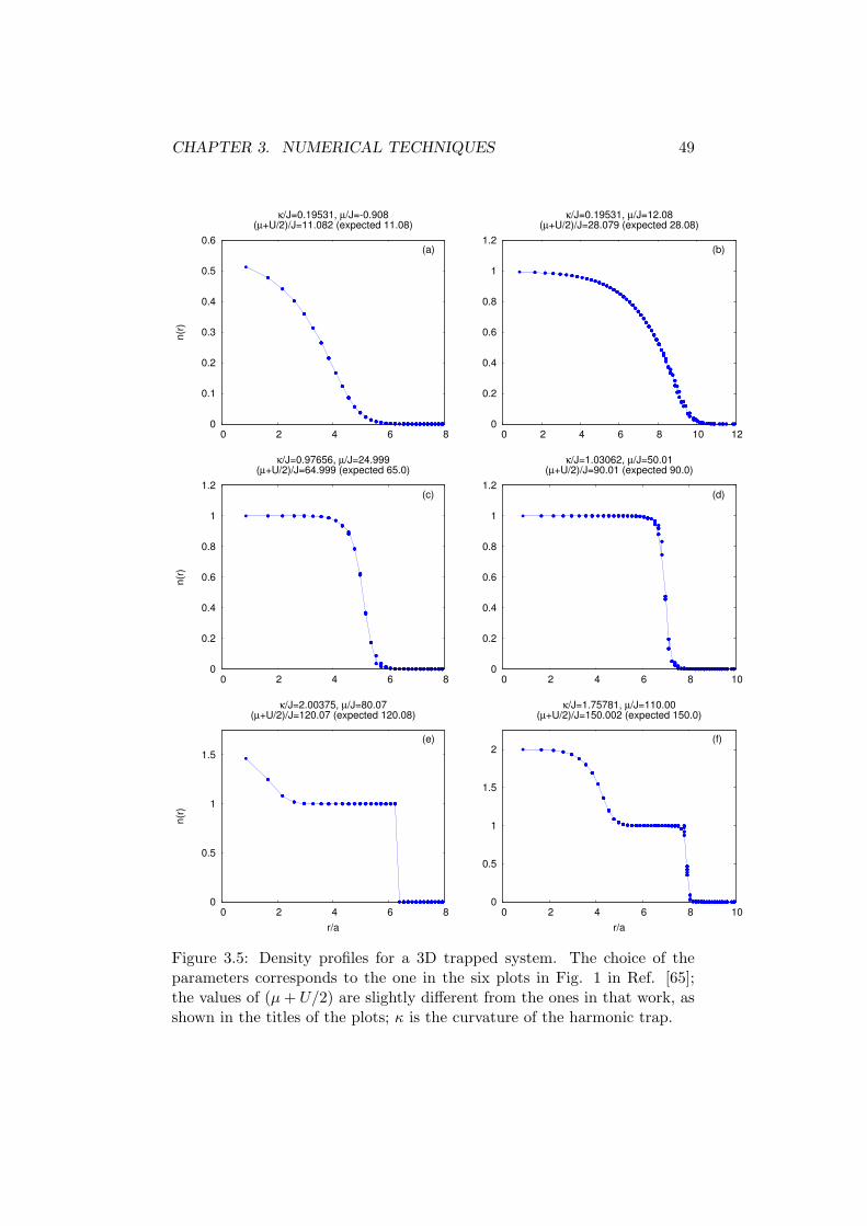
CHAPTER 3. NUMERICAL TECHNIQUES 49
0
0.1
0.2
0.3
0.4
0.5
0.6
0 2 4 6 8
n(r
)
κ/J=0.19531, µ/J=-0.908(µ+U/2)/J=11.082 (expected 11.08)
(a)
0
0.2
0.4
0.6
0.8
1
1.2
0 2 4 6 8 10 12
κ/J=0.19531, µ/J=12.08(µ+U/2)/J=28.079 (expected 28.08)
(b)
0
0.2
0.4
0.6
0.8
1
1.2
0 2 4 6 8
n(r
)
κ/J=0.97656, µ/J=24.999(µ+U/2)/J=64.999 (expected 65.0)
(c)
0
0.2
0.4
0.6
0.8
1
1.2
0 2 4 6 8 10
κ/J=1.03062, µ/J=50.01(µ+U/2)/J=90.01 (expected 90.0)
(d)
0
0.5
1
1.5
0 2 4 6 8
n(r
)
r/a
κ/J=2.00375, µ/J=80.07(µ+U/2)/J=120.07 (expected 120.08)
(e)
0
0.5
1
1.5
2
0 2 4 6 8 10
r/a
κ/J=1.75781, µ/J=110.00(µ+U/2)/J=150.002 (expected 150.0)
(f)
Figure 3.5: Density profiles for a 3D trapped system. The choice of theparameters corresponds to the one in the six plots in Fig. 1 in Ref. [65];the values of (µ+ U/2) are slightly different from the ones in that work, asshown in the titles of the plots; κ is the curvature of the harmonic trap.

CHAPTER 3. NUMERICAL TECHNIQUES 50
0
30000
60000
0 1 2 3
S(k
,0,0
)
κ/J=0.19531, µ/J=-0.908(µ+U/2)/J=11.082 (expected 11.08)
(a)
0
1e+06
2e+06
3e+06
0 1 2 3
κ/J=0.19531, µ/J=12.08(µ+U/2)/J=28.079 (expected 28.08)
(b)
0
20000
40000
60000
0 1 2 3
S(k
,0,0
)
κ/J=0.97656, µ/J=24.999(µ+U/2)/J=64.999 (expected 65.0)
(c)
0
40000
80000
0 1 2 3
κ/J=1.03062, µ/J=50.01(µ+U/2)/J=90.01 (expected 90.0)
(d)
1000
2000
3000
0 1 2 3
S(k
,0,0
)
k a
κ/J=2.00375, µ/J=80.07(µ+U/2)/J=120.07 (expected 120.08)
(e)
0
100000
200000
300000
0 1 2 3
k a
κ/J=1.75781, µ/J=110.00(µ+U/2)/J=150.002 (expected 150.0)
(f)
Figure 3.6: S(k) along a cut k = (k, 0, 0) for a 3D trapped system. Theparameters correspond to the ones in Fig. 3.5.

CHAPTER 3. NUMERICAL TECHNIQUES 51
0
500
1000
1500
2000
0 π/8 π/4 3π/8 π/2
S(k
,0,0
)
k a
N=378, κ/U=0.02, µ/U=0.400, J/U=0.0050N=803, κ/U=0.03, µ/U=1.005, J/U=0.0075N=376, κ/U=0.02, µ/U=0.401, J/U=0.0200
(x 1/25)
Figure 3.7: S(k) along a cut k = (k, 0, 0) for a 3D trapped system. Top:figure from [58] (empty symbols are results from mean-field, full ones includeperturbative corrections). Bottom: results from the present work (α ≡ κ isthe curvature of the harmonic trap).

CHAPTER 3. NUMERICAL TECHNIQUES 52
Figure 3.8: Top: integrated momentum distribution n⊥(kx, ky) along a cutk⊥ = (k, 0); figure adapted from Ref. [60]. Bottom: results from thepresent work (59×59×59 lattice, lattice depth V0/ER = 22, trap curvatureκ = 0.00131 and number of particles N = 94172), with or without theGaussian Wannier envelope.

CHAPTER 3. NUMERICAL TECHNIQUES 53
3.4 Quantum Monte Carlo
As we mentioned in section 3.1, the exponential growth of the Hilbert spacedimension D with the system size makes the computation of the exactground state wave function impossible for a large system; but even knowingthis wave function (and being able to store it on a computer) would not beenough, because computing any physical observable would require a sum-mation of D terms. We will describe here two Monte Carlo schemes thatprovide a way of dealing with this task.
The VMC approach is based on a certain choice of a trial wave func-tion, including a set of variational coefficients that have to be optimizedto minimize the expectation value of the Hamiltonian. This method de-pends heavily on the choice of the trial wave function, but despite givingonly approximate results it can provide some physical information about thesystem. Moreover it is often needed as a starting point for more accuratemethods. The GFMC scheme is a stochastic implementation of the powermethod, in which a projector operator is applied repeatedly to an initialwave function to filter out the high energy components and find the groundstate. This method is in principle exact, up to the statistical error.
3.4.1 Variational Monte Carlo
The VMC method is based on a certain choice of a trial wave function |ψα〉,depending on a set of parameters {α} and expressed in terms of a certainbasis {|x〉}. A VMC scheme includes the following operations
• computing the expectation value of the energy for a certain choice ofthe coefficients α;
• optimizing the coefficients in order to minimize this expectation value,thus obtaining the best estimate of the ground state energy and wavefunction;
• computing the relevant observables on this state.
Considering the wave function |ψ〉 (for a fixed set of parameters), the ex-pectation value of the Hamiltonian can be written as
E[ψ] =〈ψ|H|ψ〉〈ψ|ψ〉 =
∑
x eL(x)ψ2(x)
∑
x ψ2(x)
=∑
x
eL(x)px, (3.42)
by introducing the local energy
eL(x) =〈x|H|ψ〉〈x|ψ〉 (3.43)

CHAPTER 3. NUMERICAL TECHNIQUES 54
and the (normalized, non-negative) probability distribution
px =ψ2(x)
∑
y ψ2(y)
. (3.44)
Therefore, computing the energy in a state corresponds to taking the averageof the local energy eL(x), weighted with the probability distribution px. Ifwe can construct a sequence of configurations {|xn〉} distributed accordingto the probability px, then the expectation value of the local energy can becomputed as
E[ψ] = limN→∞
(
1
N
N∑
n=1
eL(xn)
)
. (3.45)
One way of sampling the sequence of states {|xn〉} in such a way thatthe states are distributed according to the probability p(x) is the one basedon the Metropolis algorithm (Ref. [81]), in which a move from an initialstate |xi〉 to a final state |xf 〉 is proposed with a rate
T (xi → xf ) = T (xf → xi), (3.46)
and accepted with probability
A(xi → xf ) = min
(
1,p(xf )
p(xi)
)
= min
(
1,
∣
∣
∣
∣
〈xf |ψ〉〈xi|ψ〉
∣
∣
∣
∣
2)
. (3.47)
This scheme satisfies the “detailed balance” condition
p(xi)T (xi → xf )A(xi → xf ) = p(xf )T (xf → xi)A(xf → xi). (3.48)
With this procedure, it is possible to use Eq. (3.45) to compute E[ψα]for any choice of the coefficients {α} of the trial wave function |ψα〉.
The next step consists in finding the optimal set of α’s, for which E[ψα]is minimum. We will now describe an example of the simplest case, in whichthe wave function depends only on one coefficient (g) and the optimal statecan be estimated by directly comparing the energies for different values ofg. More efficient optimization schemes have to be used for variational wavefunctions depending on a larger number of parameters.
Example
Here we give an example of the explicit calculation of the terms in the localenergy in a simple case. We consider the homogeneous Bose-Hubbard for afixed number N of bosons
H = −J2
L∑
i=1
(
b†i bi+1 + b†i+1bi
)
+U
2
L∑
i=1
ni(ni − 1), (3.49)
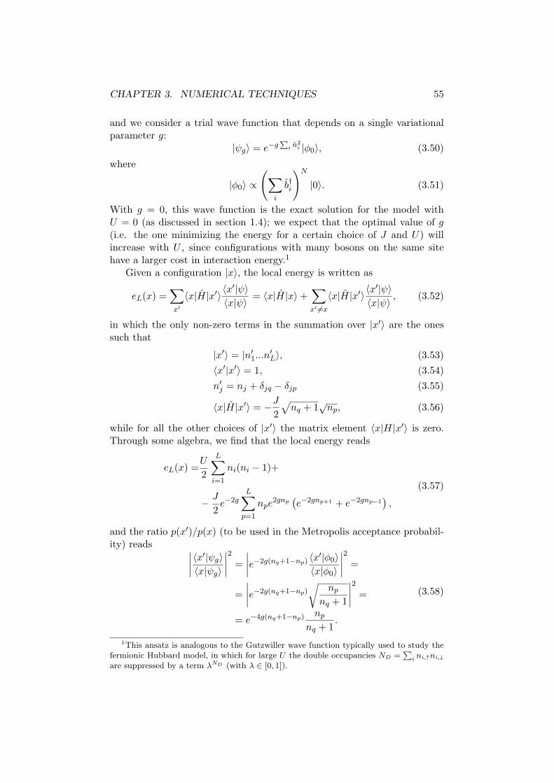
CHAPTER 3. NUMERICAL TECHNIQUES 55
and we consider a trial wave function that depends on a single variationalparameter g:
|ψg〉 = e−g∑
i n2i |φ0〉, (3.50)
where
|φ0〉 ∝(
∑
i
b†i
)N
|0〉. (3.51)
With g = 0, this wave function is the exact solution for the model withU = 0 (as discussed in section 1.4); we expect that the optimal value of g(i.e. the one minimizing the energy for a certain choice of J and U) willincrease with U , since configurations with many bosons on the same sitehave a larger cost in interaction energy.1
Given a configuration |x〉, the local energy is written as
eL(x) =∑
x′
〈x|H|x′〉〈x′|ψ〉
〈x|ψ〉 = 〈x|H|x〉+∑
x′ 6=x〈x|H|x′〉〈x
′|ψ〉〈x|ψ〉 , (3.52)
in which the only non-zero terms in the summation over |x′〉 are the onessuch that
|x′〉 = |n′1...n′L〉, (3.53)
〈x′|x′〉 = 1, (3.54)
n′j = nj + δjq − δjp (3.55)
〈x|H|x′〉 = −J2
√
nq + 1√np, (3.56)
while for all the other choices of |x′〉 the matrix element 〈x|H|x′〉 is zero.Through some algebra, we find that the local energy reads
eL(x) =U
2
L∑
i=1
ni(ni − 1)+
− J
2e−2g
L∑
p=1
npe2gnp
(
e−2gnp+1 + e−2gnp−1)
,
(3.57)
and the ratio p(x′)/p(x) (to be used in the Metropolis acceptance probabil-ity) reads
∣
∣
∣
∣
〈x′|ψg〉〈x|ψg〉
∣
∣
∣
∣
2
=
∣
∣
∣
∣
e−2g(nq+1−np) 〈x′|φ0〉〈x|φ0〉
∣
∣
∣
∣
2
=
=
∣
∣
∣
∣
e−2g(nq+1−np)√
npnq + 1
∣
∣
∣
∣
2
=
= e−4g(nq+1−np) npnq + 1
.
(3.58)
1This ansatz is analogous to the Gutzwiller wave function typically used to study thefermionic Hubbard model, in which for large U the double occupancies ND =
∑ini,↑ni,↓
are suppressed by a term λND (with λ ∈ [0, 1]).

CHAPTER 3. NUMERICAL TECHNIQUES 56
Figure 3.9: Variational energy for a system of 8 bosons on 8 sites, as afunction of the coefficient g. J is set equal to 1, U is different in the fourplots. The optimal energy is marked with a full circle. The statistical errorsare smaller than the symbols.
Eqs. (3.57) and (3.58) are the basis for a VMC approach. In this case weuse a trivial optimization scheme, i.e. we compute the energy for differentchoices of the variational parameter g in a mesh. Results for different valuesof U are shown in Fig. 3.9, from which it can be noticed that the optimalvalue of g is larger when the on-site repulsive interaction is stronger. Thisis an example of a situation in which a physical information (i.e. the factthat for larger U the multiple occupancies are suppressed) is already clearfrom a variational approach, while in a more sophisticated (and accurate)approach this might not be directly available.
Remarks
In the previous example we have used a trivial optimization scheme to findthe optimal g; more efficient schemes have to be used for variational wavefunctions depending on a larger number of parameters. In particular theVMC calculation on which the results in chapter 5 are based makes use ofthe stochastic optimization algorithm introduced in Ref. [82].
We stress that the applicability of a VMC approach of this kind to the

CHAPTER 3. NUMERICAL TECHNIQUES 57
model of interest is based on the fact that (a) for each state |x〉 there isa limited number (of the order of the number of sites) of non-zero matrixelements 〈x|H|x′〉 and (b) there is an efficient way of computing these matrixelements.
A general feature of VMC is the so called zero variance property, i.e.in case the chosen trial wave function is an eigenstate of the Hamiltonianthen the fluctuations of the local energy are identically zero (eL(x) does notdepend on |x〉). This is specially useful when some analytical results areknown, in order to validate the QMC approach.
3.4.2 Green’s Function Monte Carlo
The GFMC technique is a stochastic implementation of the power method,in which a projector operator is applied repeatedly to an initial wave func-tion to filter out the high energy components and find the ground state.In this section we first introduce the power method and then describe thesimpler version of GFMC (the single walker formulation). A more detailedexplanation can be found in Ref. [83].
Power method
Given an initial state |ψ0〉 that is not orthogonal to the ground state (i.e.such that 〈ψ0|ψGS〉 6= 0), we show how to construct a sequence of statesconverging to |ψGS〉. We define this sequence as
〈x|ψn+1〉 =∑
x′
(
Λδx,x′ − 〈x|H|x′〉)
〈x′|ψn〉, (3.59)
where Λ is a positive number. Considering a basis of eigenstates |φi〉 of theHamiltonian
H|φi〉 = Ei|φi〉, (3.60)
we rewrite the initial state of the sequence as
|ψ0〉 =∑
i
|φi〉〈φi|ψ0〉. (3.61)
For the first iteration in the sequence we have
〈x|ψ1〉 =∑
i
∑
x′
(
Λδx,x′ − 〈x|H|x′〉)
〈x′|φi〉〈φi|ψ0〉 =
=∑
i
(
Λ〈x|φi〉 − 〈x|H|φi〉)
〈φi|ψ0〉 =
=∑
i
〈φi|ψ0〉(Λ− Ei)〈x|φi〉,
(3.62)

CHAPTER 3. NUMERICAL TECHNIQUES 58
and the n-th state reads
|ψn〉 =∑
i
〈φi|ψ0〉(Λ− Ei)n|φi〉. (3.63)
If Λ is large enough, we have that
|Λ− EGS | = maxi
|Λ− Ei| , (3.64)
and all the components of ψn not corresponding to the ground state areexponentially suppressed for large n. Thus we have proved that the sequenceconverges to the ground state: |ψn〉 → |ψGS〉.
We stress that this method does not include any approximation, but itcannot be applied in practice because the number of basis states |x〉 of whichone has to keep track grows exponentially when new states are generated byusing Eq. (3.63).
Single walker GFMC
The goal of this technique is to reproduce the power method in a stochasticway, in which we do not need to keep track of an exponentially increasingnumber of states; this is achieved by performing the n-th step of a powermethod
〈x|ψn〉 = 〈x|(Λ− H)n|ψ0〉 (3.65)
in a stochastic way. The basic element of this approach is the so calledwalker, that is determined by a state |x〉 and a weight w ≥ 0. Given an initialwalker configuration (x0, w0), we introduce a rule to generate (xn+1, wn+1)in terms of (xn, wn); this defines a Markov chain with elements distributedwith a probability Pn(xn, wn). In order to use this chain to evaluate ψn(x),we require that
∫
dwwPn(x,w) = 〈x|ψn〉, (3.66)
so that for n→ ∞ we have a way of getting to the ground state, even thoughwe are only interested in computing expectation values and not in 〈x|ψGS〉itself.
In order to construct the correct Markov chain, we introduce the Green’sfunction
Gx′,x = Λδx′,x − 〈x′|H|x〉 (3.67)
and we have to assume that Gx′,x ≥ 0 so that it can be interpreted as aprobability. For the diagonal terms Gx,x, we can choose Λ large enoughto satisfy this requirement, but the off-diagonal terms Gx′,x only dependon the Hamiltonian. If the requirement of Gx′,x ≥ 0 is not satisfied, theHamiltonian has the so called sign problem (typically present for fermionic
CHAPTER 3. NUMERICAL TECHNIQUES 59
Hamiltonians or in frustrated lattices) and the approach described here can-not be directly used. Once we assume that there is no sign-problem, we cansplit G in the following way
bx =∑
x′
Gx′,x,
px′,x =Gx′,xbx
,
Gx′,x = px′,xbx,
(3.68)
so that px′,x is a stochastic matrix (i.e. px′,x ≥ 0 and∑
x′ px′,x = 1). Thisdecomposition of Gx′,x allows us to construct the Markov chain by definingthe following rules for generating (xn+1, wn+1) from (xn, wn)
• generate xn+1 with probability pxn+1,xn ,
• multiply the old weight by bxn to obtain the new one: wn+1 = wnbxn .
It can be proven that the resulting Markov chain satisfies Eq. (3.66).
Importance sampling
The present GFMC scheme does not satisfy the zero variance property,that in turn is satisfied by the VMC scheme described in section 3.4.1. Thisproperty corresponds to the fact that if the variational wave function is anexact eigenstate of the Hamiltonian then the local energy eL(x) is a constant(not depending on |x〉) and it has no statistical fluctuations. In order torecover this property in the GFMC scheme, we consider the importancesampling Green’s function
Gx′,x = Gx′,xψg(x
′)ψg(x)
, (3.69)
where the so called guiding function ψg is a guess of the ground state wavefunction, obtained before using the GFMC (for instance this can be theoutcome of a VMC calculation). The same decomposition of Eq. (3.68) canbe applied to G
Gx′,x = px′,xbx,
px′,x =Gx′,xbx
,
bx =∑
x′
Gx′,x = Λ−∑
x′ ψg(x′)Hx′,x
ψg(x)= Λ− eL(x),
(3.70)
and the Markov chain can be defined in the same way. With these definitions,if the guiding function is the correct ground state wave function (ψg(x) =ψGS(x)) we have that the local energy eL(x) is a constant and statisticalfluctuations vanish. Thus we have recovered the zero variance property.

CHAPTER 3. NUMERICAL TECHNIQUES 60
Observables
The ground state energy is obtained as the large n limit of the weightedaverage of the local energies, i.e.
EGS = limn→∞
〈wneL(xn)〉〈wn〉
= limn→∞
〈ψg|H(Λ− H)n|φ〉〈ψg|(Λ− H)n|φ〉
, (3.71)
where |φ〉 is defined as the state such that 〈x|φ〉 ≡ bxψg(x).In practice, it is enough to stop the iteration at a finite number of itera-
tions n = n. In order to have a statistically relevant expectation value, onecould generate many Markov chains of n steps and consider their average.However, it is more convenient to generate a single Markov chain ofM steps(with M ≫ n) and use the expression
EGS = limn→∞
〈ψg|H(Λ− H)n|φ〉〈ψg|(Λ− H)n|φ〉
=
M∑
n=n0
Gn,neL(xn)
M∑
n=n0
Gn,n
, (3.72)
where n0 is the number of steps required to get to the equilibrium and thecoefficients Gn,n are defined as
Gn,n =
n∏
i=1
bxn−i. (3.73)
In Fig. 3.10 the result of such a calculation for the Hamiltonian in Eq. (1.42)is compared with the exact value, to show the convergence in terms of n.
We now consider other observables; if they are diagonal in the occupationnumber basis, the analogue of the local energy is just the correspondingeigenvalue
〈ψg|A|x〉〈ψg|x〉
= Ax. (3.74)
It can be verified that the analogue of Eq. (3.71) is
〈wnAxn−m〉
〈wn〉=
〈ψg|(Λ−H)mA(Λ−H)n−m|φ〉〈ψg|(Λ−H)n|φ〉 , (3.75)
where n−m is the iteration at which the operator is applied. Thus Eq. (3.72)becomes
〈ψGS |A|ψGS〉 ≃
M∑
n=n0
Gn,nAxn−m
M∑
n=n0
Gn,n
, (3.76)

CHAPTER 3. NUMERICAL TECHNIQUES 61
Figure 3.10: Points: GFMC energy (Eq. 3.72) of the Hamiltonian inEq. (1.42), as a function of n. The solid horizontal line corresponds to theexact energy, computed by the ED scheme described in section 3.1. Systemof 8 bosons on 8 sites, with (J, U, V ) = (1, 5, 4).
that is valid for n≫ 1 and m≫ 1.The scheme described here can be generalized to use many walkers si-
multaneously. If one wants to keep the number of walkers fixed, a reconfig-uration scheme has to be used to avoid that a few walkers gain a very largeweight compared to the others. The results shown in chapter 5 are obtainedthrough a many-walkers GFMC scheme that makes use of the stochasticreconfiguration technique (see Ref. [84]).

Chapter 4
Trapped model: mean-field
results
In this chapter, we show the results of the mean-field approach described insection 3.2.2 for the trapped Bose-Hubbard model. In particular, we measurethe visibility of the quasimomentum distribution (introduced in section 2.1)and we describe which features are found in the mean-field results.
In section 4.1, we consider a 1D system and we show how the choice ofdifferent trapping potentials leads to different visibility curves. The resultsfor 2D systems are shown in section 4.2, where we describe both a pure 2Dsystem and a 2D system that constitutes the central layer of a 3D one.
4.1 1D system
In this section we show the results of our calculations in a one-dimensionalsystem. In particular we have studied (for different values of U/J) thefollowing two systems
• system of N = 80 bosons in Ns = 79 lattice sites, trapping potentialVT (i) = (0.06 J) i2;
• system of N = 80 bosons in Ns = 79 lattice sites, trapping potentialVT (i) = (0.003 U) i2.
Throughout this section we set the lattice constant a to one.In the weakly interacting regime (small U/J) the entire system is in
the superfluid phase; for larger values of U/J , we observe the formationof the Mott domains with n = 1; for even stronger interactions, the twoMott regions with n = 2 appear around the central superfluid domain, andthey get connected when the interactions increase further. The first way ofobserving this phase structure comes by looking at the local density profileni, that is pinned to integer values in the Mott domains (examples are shown
62
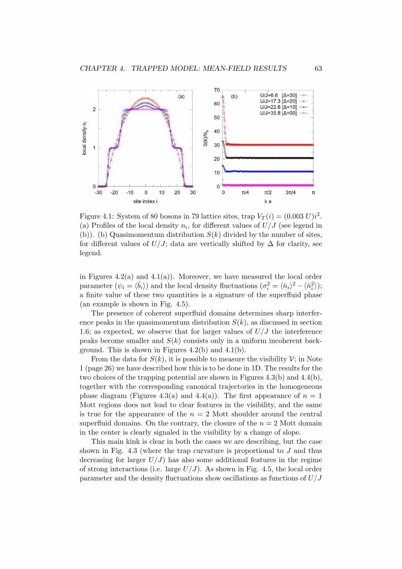
CHAPTER 4. TRAPPED MODEL: MEAN-FIELD RESULTS 63
Figure 4.1: System of 80 bosons in 79 lattice sites, trap VT (i) = (0.003 U)i2.(a) Profiles of the local density ni, for different values of U/J (see legend in(b)). (b) Quasimomentum distribution S(k) divided by the number of sites,for different values of U/J ; data are vertically shifted by ∆ for clarity, seelegend.
in Figures 4.2(a) and 4.1(a)). Moreover, we have measured the local orderparameter (ψi = 〈bi〉) and the local density fluctuations (σ2i = 〈ni〉2−〈n2i 〉);a finite value of these two quantities is a signature of the superfluid phase(an example is shown in Fig. 4.5).
The presence of coherent superfluid domains determines sharp interfer-ence peaks in the quasimomentum distribution S(k), as discussed in section1.6; as expected, we observe that for larger values of U/J the interferencepeaks become smaller and S(k) consists only in a uniform incoherent back-ground. This is shown in Figures 4.2(b) and 4.1(b).
From the data for S(k), it is possible to measure the visibility V; in Note1 (page 26) we have described how this is to be done in 1D. The results for thetwo choices of the trapping potential are shown in Figures 4.3(b) and 4.4(b),together with the corresponding canonical trajectories in the homogeneousphase diagram (Figures 4.3(a) and 4.4(a)). The first appearance of n = 1Mott regions does not lead to clear features in the visibility, and the sameis true for the appearance of the n = 2 Mott shoulder around the centralsuperfluid domains. On the contrary, the closure of the n = 2 Mott domainin the center is clearly signaled in the visibility by a change of slope.
This main kink is clear in both the cases we are describing, but the caseshown in Fig. 4.3 (where the trap curvature is proportional to J and thusdecreasing for larger U/J) has also some additional features in the regimeof strong interactions (i.e. large U/J). As shown in Fig. 4.5, the local orderparameter and the density fluctuations show oscillations as functions of U/J

CHAPTER 4. TRAPPED MODEL: MEAN-FIELD RESULTS 64
Figure 4.2: System of 80 bosons in 79 lattice sites, trap VT (i) = (0.06 J)i2.(a)-(b): same as in caption of Fig. 4.1.
in the region where the local density is between 0 and 1. This effect is due tothe competition between the trapping energy (that pushes bosons towardsthe center) and the on-site repulsion, and it has strong consequences on thevisibility (that is larger when more bosons are in the superfluid regions).In the other case (i.e. when the trap frequency is proportional to U , thusgetting larger for increasing U/J), the visibility decay is smooth, after thekink; no oscillations are observed in the local order parameter and in thedensity fluctuations, and in fact no oscillations are present in the visibility.
As reviewed in section 2.3, an effect similar to these oscillations is ob-served in the QMC study in Ref. [50] (in which a trap curvature proportionalto J is used). Note that the oscillations observed here originate from theoscillations in the superfluid regions with 0 < n < 1, whereas the ones inRef. [50] are explained by the change of size of the superfluid regions with1 < n < 2; however the mechanism is the same and it is based on the inter-play between the trapping potential and the on-site repulsion that leads toa certain density structure. It has to be stressed that in 1D the QMC andmean-field phase diagrams are qualitatively different, thus a quantitativeagreement between the two methods is not expected.
Our observations lead to the conclusion that the influence of differenttrapping potentials on the density structure (given by the competition withthe repulsive interaction) has an effect also on the visibility of the system.This is clear by looking at the regime of large U/J in our results, while inthe weakly interacting regime the visibility features are similar for the twochoices of the trap.

CHAPTER 4. TRAPPED MODEL: MEAN-FIELD RESULTS 65
Figure 4.3: System of 80 bosons in 79 lattice sites, trap VT (i) = (0.06 J)i2.(a) Open circles represent (zJ/U, µ/U) points in the homogeneous mean-fieldphase diagram; µ is the external chemical potential, z = 2 is the numberof nearest neighbours of each site. (b) Visibility of the quasimomentumdistribution, computed as described in Note 1 (page 26).
Figure 4.4: System of 80 bosons in 79 lattice sites, trap VT (i) = (0.06 J)i2.(a)-(b): same as in caption of Fig. 4.3.

CHAPTER 4. TRAPPED MODEL: MEAN-FIELD RESULTS 66
Figure 4.5: System of 80 bosons in 79 lattice sites, trap VT (i) = (0.06 J)i2.Plots of the local density fluctuations σ2i (a) and the local order parametersquared: ψ2
i (b) , both as functions of U/J .

CHAPTER 4. TRAPPED MODEL: MEAN-FIELD RESULTS 67
4.2 2D system
When considering a 2D system, we choose the parameters of the model tobe relevant for a comparison with experiments. In particular we considera system in an isotropic trapping potential with frequency as in Eq. (1.34),where the external magnetic trap has ωm = 30 Hz×2π, m = 86.9 a.u. is themass of the 87Rb atoms and w = 100 µm is the waist of the laser beamsgenerating the lattice. The way of obtaining 2D independent system ina 3D experimental set-up is that of setting the lattice depth in the thirddirection to a large value (V0,z = 28.8ER), so that the hopping along zis strongly suppressed and all the layers are effectively independent. Thewave length of the laser beams forming the lattice is the same in the threedirections (λ = 1064 nm) and the lattice depth along x and y is the same(V0 ≡ V0,x = V0,y).
1
For each choice of V0, the parameters of the Bose-Hubbard model (theon-site interaction U and the hopping coefficient J in the x-y plane) arecomputed as explained in sections 1.2 and 1.3.
First case
As a first case, we study a trapped 2D system and we do not consider it as apart of a 3D set-up. Thus we choose a fixed number of particles (N = 2600),that remains constant for different lattice depths V0. When we let V0 vary,we observe the formation of the shell structure described in section 1.5; thisis shown in Fig. 4.6. Note that we can study the density profile as a functionof the distance r from the center, because of the symmetry of the trappingpotential under rotations in the x-y plane.
This shell structure can be studied globally by measuring the number ofbosons in the Mott and superfluid phases. In order to recognize the phaseon a certain site, we check whether the local order parameter ψi is finite orvanishing. This is done by setting a finite tolerance ε and by checking thecondition ψ2
i < ε; if the condition is true, we consider the site as hostingparticles in the Mott phase. Note that in this procedure (required by thefact that the numerical value of ψi remains small but finite even in the Mottphase) the choice of ε is arbitrary, thus the results have to be consideredonly qualitatively. As shown in Fig. 4.7, in the regime of weak interactionsall the particles are in the superfluid phase, while for increasing lattice depthmore particles become part of the Mott shells. It is clear from the data thatthe increase in the number of “Mott particles” is steeper for certain values ofV0/ER, corresponding to the formation of the different Mott domains; withthe help of the density profiles shown in Fig. 4.6, it is possible to explain
1The parameters that we have listed here are comparable to the ones used in currentexperiments with optical lattices; in particular, they are relevant for a set-up used inAndreas Hemmerich’s group at the Institut fur Laserphysik (Hamburg, Germany).

CHAPTER 4. TRAPPED MODEL: MEAN-FIELD RESULTS 68
some of these features. For V0 ≃ 14.75ER the Mott shell with n = 3 startsto form around the central superfluid domain, and this corresponds to asudden increase in the number of particles in the Mott state. The othersteep increase in this quantity is for V0 ≃ 15.5ER, corresponding to theclosure of the Mott domain in the center.
In Fig. 4.8, we show the visibility V (computed as in Eq. (2.5)) and itsnumerical derivative. By looking at the derivative, it is possible to recognizesome features in V. In particular for V0/ER ≃ 14.75 and V0/ER ≃ 15.5 thevisibility has some kinks, in which its decay is steeper; these correspond tothe features previously recognized in the density profiles and in Fig. 4.7.A different feature takes place at V0/ER ≃ 16.85; this is a point at whichthe decay of V is less steep (whereas the previous features have the oppo-site behaviour). The explanation is that at this value of V0 the number ofparticles in the Mott state decreases (as seen in Fig. 4.7), before increasingagain. For this reason, the decay of V “slows down” around that point. Notethat the fact that the number of particles in the Mott state is not alwaysmonotonously increasing with V0 is not contradictory, since also the trap-ping potential depends on V0 and it competes with the repulsive interactionin redistributing the particles in the system.
Figure 4.6: Radial dependence of the local density n(r) (blue full circles)and local order parameter ψ(r) (red empty squares). The four plots are forV0/ER = 14.25, 14.75, 15.25, 15.5 (ordered row by row).

CHAPTER 4. TRAPPED MODEL: MEAN-FIELD RESULTS 69
0
600
1200
1800
2400
10 11 12 13 14 15 16 17 18
V0/ER
number of bosons in MI state
number of bosons in SF state
Figure 4.7: Number of particles in the two phases (Mott insulator and su-perfluid) for a 2D system with N = 2600 bosons, as a function of the latticedepth in the x-y plane.
0.4
0.5
0.6
0.7
0.8
0.9
1
10 11 12 13 14 15 16 17 18
-0.4
-0.2
0
0.2
0.4
vis
ibili
ty
derivative
V0/ER
Figure 4.8: Visibility (upper curve) and its numerical derivative (lowercurve) for a 2D system with N = 2600 bosons, as functions of the latticedepth in the x-y plane.
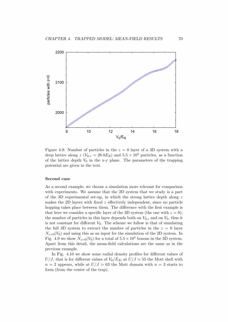
CHAPTER 4. TRAPPED MODEL: MEAN-FIELD RESULTS 70
2000
2100
2200
8 10 12 14 16 18
part
icle
s w
ith z
=0
V0/ER
Figure 4.9: Number of particles in the z = 0 layer of a 3D system with adeep lattice along z (V0,z = 28.8ER) and 5.5 × 10⁴ particles, as a functionof the lattice depth V0 in the x-y plane. The parameters of the trappingpotential are given in the text.
Second case
As a second example, we choose a simulation more relevant for comparisonwith experiments. We assume that the 2D system that we study is a partof the 3D experimental set-up, in which the strong lattice depth along zmakes the 2D layers with fixed z effectively independent, since no particlehopping takes place between them. The difference with the first example isthat here we consider a specific layer of the 3D system (the one with z = 0);the number of particles in this layer depends both on V0,z and on V0, thus itis not constant for different V0. The scheme we follow is that of simulatingthe full 3D system to extract the number of particles in the z = 0 layerNz=0(V0) and using this as an input for the simulation of the 2D system. InFig. 4.9 we show Nz=0(V0) for a total of 5.5× 10⁴ bosons in the 3D system.Apart from this detail, the mean-field calculations are the same as in theprevious example.
In Fig. 4.10 we show some radial density profiles for different values ofU/J , that is for different values of V0/ER; at U/J ≃ 55 the Mott shell withn = 2 appears, while at U/J ≃ 63 the Mott domain with n = 3 starts toform (from the center of the trap).

CHAPTER 4. TRAPPED MODEL: MEAN-FIELD RESULTS 71
As in the previous section, some kinks in the visibility (Fig. 4.11) corre-spond to these specific points. Note that the first kink is slightly shifted tolarger U/J w.r.t. to the point U/J ≃ 63 at which the Mott domain appearsin the center; this means that the kink in the visibility corresponds to thesituation in which the size of this domain becomes relevant.The trajectory corresponding to the chosen parameters enters the n = 3Mott lobe close to its tip, in the homogeneous phase diagram (not shown);for this reason, the kink in the visibility corresponding to the closure of theMott in the center of the trap is close to the expected mean-field value forthe tip of the lobe (see vertical line in Fig. 4.11).For large values of U/J , the sizes of the superfluid shells with densityn ∈ [1, 2] and n ∈ [0, 1] have an oscillating behaviour as functions of U/J ;as explained in section 4.1, this is an effect of the interplay between thetrap and the repulsion, and it is linked to the features in the visibility forU/J & 90.
Figure 4.10: Radial dependence of the local density n(r) (blue full circles)and local order parameter ψ(r) (red empty squares). The four plots arefor U/J = 46.2, 55.6, 64.3, 74.9 (ordered row by row), corresponding toV0/ER = 13.25, 14, 14.6, 15.25.

CHAPTER 4. TRAPPED MODEL: MEAN-FIELD RESULTS 72
0.6
0.7
0.8
0.9
1
15 30 45 60 75 90 105 120
-0.04
-0.02
0
0.02
vis
ibili
ty
derivative
U/zJ
Figure 4.11: Visibility (upper curve) and its numerical derivative (lowercurve) for a 2D system with varying number of bosons, as functions of thedimensionless ratio U/J . The vertical dashed line corresponds to U/J =55.71, the tip of the lobe for the homogeneous system in the mean-fieldapproach (see Ref. [57]). The x-axis range corresponds approximately toV0/ER ∈ [8, 17.3]; for large U/J the derivative of V has strong oscillationsand it is not shown here.

Chapter 5
Extended model: QMC
results
In this chapter we show the results of our QMC simulations of the one-dimensional extended Bose-Hubbard model (Eq. 1.42). First we have verifiedthat the GFMC code used here is able to reproduce exact results, obtainedthrough exact diagonalization; this is described in section 5.1. In section5.2 we show our results in the characterization of the different phases of the1D extended Bose-Hubbard model. In particular, we describe the differencebetween the two insulating phases (Mott and Haldane insulators) and weverify numerically an analytic estimate (from Ref. [85]) of the way in whichthe parity order parameter decays in the superfluid phase.
The numerical approach that we use is the GFMC scheme described insection 3.4.2. As a guiding wave function for the importance sampling, wechose the following wave function |ψ〉 for a system of N bosons
|ψ〉 = exp
1
2
∑
i,j
vijninj
|φ0〉, (5.1)
where |φ0〉 is the condensate wave function
|φ0〉 ∝(
∑
i
b†i
)N
|0〉. (5.2)
This choice of |ψ〉 is also used – for instance – in Ref. [68]. The operatorthat is applied on |φ0〉 is a Jastrow factor that introduces a correlationbetween the sites i and j, depending on the coefficient vij . We assumethat the coefficients vij depend only on the distance |i − j|, because of thetranslational invariance of the Hamiltonian Eq. (1.42). Note that PeriodicBoundary Conditions are required to have the full translational invariance;this means that the sites 1 and Ns are seen as nearest neighbours.
73

CHAPTER 5. EXTENDED MODEL: QMC RESULTS 74
Figure 5.1: Difference of the ground state energy computed by GFMC andits exact value; system of 8 bosons on 8 sites, with J = 1 and U = 5. V isthe next-nearest-neighbour repulsion, as in Eq. (1.42).
VMC and stochastic minimization have been used to find the optimalcoefficients vij , before using |ψ〉 as a guiding function in the GFMC scheme.Note that the presence of a trapping potential would require some modi-fications of this approach, since the homogeneity of the system would beexplicitly broken by VT (x). A first solution would be that of consideringthe coefficients vij explicitly dependent on the sites i and j. Note that thiswould increase the number of variables in the VMC optimization, from Ns/2(the number of inequivalent distances for Ns even) to N
2s (the total number
of pairs of sites).
5.1 Validation of the GFMC scheme
In order to validate our GFMC approach, we have compared the resultswith the exact ones, obtained through ED on small lattices. In Fig. 5.1 weshow a comparison of the ground state energy computed through GFMCwith the exact one. The results are in good agreement; the error bars couldbe reduced further by using a larger number of walkers or of MC steps.
The same comparison is shown in Fig. 5.2 for the three order param-eters defined in Eqs (1.46) (string order parameter), (1.45) (parity orderparameter) and (1.44) (density wave order parameter). Also in this case,the difference between GFMC results and exact ones is of the order of thestatistical error bars.

CHAPTER 5. EXTENDED MODEL: QMC RESULTS 75
Figure 5.2: Comparison of GMFC and exact results for the string, parity anddensity wave order parameter in a system of 8 bosons on 8 sites; results forJ = 1, U = 5 and varying next-nearest-neighbour repulsion V . Left: resultsof ED (empty circles) and GFMC (crosses); right: difference between exactresults and GFMC ones, including the statistical errors of GFMC. Dashedlines are guides to the eye.

CHAPTER 5. EXTENDED MODEL: QMC RESULTS 76
5.2 Results
We consider systems at unitary filling (N = Ns), for different sizes and fordifferent parameters J, U, V . In particular we consider three points in thephase diagram, with J and U fixed (J = 1 and U = 5). We let V vary, sothat (according to the phase diagram shown in Fig. 1.9) the system is inthree different phases: Mott insulator (for V = 2.8), Haldane insulator (forV = 3.2) and density wave phase (for V = 3.65).
Compared to the ED approach, GFMC allows the study of larger sys-tems. For each choice of the parameters, we have repeated the simulationfor systems of different sizes, in order to extrapolate the results to the ther-modynamic limit. In Fig. 5.3, the size scaling is shown for the parity andstring order parameters; in Fig. 5.4 the same is shown for the density waveorder parameter.
The results clearly indicate the following characterization of the groundstate of the system for different choices of V :
• for V = 2.8 the parity order parameter is non-zero while the otherones (string and density wave) vanish, therefore the system is in aMott insulating phase;
• for V = 3.2 the string order parameter is non-zero while the other ones(parity and density wave) vanish, therefore the system is in a Haldaneinsulating phase;
• for V = 3.65, the three order parameters (string, parity and densitywave) are non-zero, therefore the system is in a density wave phase.
5.2.1 Insulating phases
It is of particular interest to consider the difference between the two in-sulating phases. In both cases, there is no density wave order; however,the Haldane phase has a non-vanishing string order parameter, that cor-responds to a hidden antiferromagnetic ordering. As represented in Fig.5.5, the hidden order +,−,+,−, .. is the one that would be found after re-moving all the sites with n = n (i.e. with δn = 0). The link between anon-vanishing string order parameter and the hidden antiferromagnetic or-der in the Haldane phase is the following: if one cancels all the sites withn = n (represented as zeros in the figure), all the sites left are occupied byn = 0 or n = 2 bosons. Thus the exponential that appears in the definitionof the string order parameter (Eq. 1.46) only contributes a global sign, and

CHAPTER 5. EXTENDED MODEL: QMC RESULTS 77
Figure 5.3: Size-scaling of the string (top) and parity (bottom) order param-eters in three different phases: Mott insulator (squares), Haldane insulator(circles), density wave (triangles). The scale is logarithmic for both axis;the error bars are smaller than symbol sizes, when not explicitly shown; thedashed lines are guides to the eye.

CHAPTER 5. EXTENDED MODEL: QMC RESULTS 78
Figure 5.4: Size-scaling of the density wave order parameter in three differentphases: Mott insulator (squares), Haldane insulator (circles), density wave(triangles).The error bars are smaller than symbol sizes, when not explicitlyshown; the dashed lines are guides to the eye.
Figure 5.5: Typical configuration in the Haldane phase (a) and Mott phase(b). Average filling is one, the symbol + (−) corresponds to n = 2 (n = 0).Figure extracted from Ref. [9].
one is left with
Cstr(r) ≡⟨
δnj exp
iπ
j+r−1∑
p=j
δnp
δnj+r
⟩
=
=
⟨
δnj
j+r−1∏
p=j
(−1)δnp
δnj+r
⟩
=
= (−1)r−1 〈δnjδnj+r〉 == CDW(r).
(5.3)
Thus when there are no sites with n = n the string and density wave orderparameters are equivalent. On the contrary, the Mott phase shows nothidden order; the reason for the non-vanishing parity order parameter isthat the Mott state corresponds to an admixture of particle-hole pairs on

CHAPTER 5. EXTENDED MODEL: QMC RESULTS 79
top of the fixed-density background (see Refs [31, 12]).
5.2.2 Superfluid phase
In the superfluid phase, the large fluctuations in the occupation number (seesection 1.4) prevent the system from developing any string or parity order.In particular, the parity order parameter is expected to decay according tothe following power law (from Ref. [85])
Cpar(r) ∼ r−παn, (5.4)
where n is the average filling. The coefficient α is related to the density-density correlation function in Fourier space
N(q) ≡ 〈n−qnq〉 =1
Ns
⟨
∑
i,j
e−iq(xi−xj)ninj
⟩
; (5.5)
in the superfluid phase, this correlation function is linear for small values ofq and α is the coefficient in N(q) ≃ |α|q.
For J = 1 and V = 0, the Mott transition is expected around U =3.61 ± 0.01 (see Ref. [34]). In Figures 5.6 and 5.7 we show the results forN(q) and Cpar(r) at U = 2.5 and U = 3, that is in the superfluid phase.The values of α from the different fits are shown in Table 5.1.
U = 2.5 U = 3
α from fit of N(q) 0.434± 0.003 0.3833± 0.0016α from fit of Cpar(r) 0.436± 0.013 0.391± 0.008
Table 5.1: Results for α.
As shown in Fig. 5.7, the parity correlator at large distance has strongfluctuations; this is also due to finite size effects. Moreover, different rangesfor the fit can be chosen, thus including some arbitrariness in the results.The study of larger systems and a better statistics (i.e. a larger number ofGFMC walkers and Monte Carlo steps) would reduce the statistical errorsand make this arbitrariness less relevant. Despite these remarks, the resultsfor α are in agreement, thus proving the statement in Ref. [85].

CHAPTER 5. EXTENDED MODEL: QMC RESULTS 80
Figure 5.6: Density-density correlation function in Fourier space (Eq. 5.5)for a system of 100 bosons on 100 sites with J = 1. Results for U = 2.5 (top)and U = 3 (bottom). Fit range: q ∈ [0, 0.4]. Statistical errors (generallysmaller than the symbol sizes) are shown.

CHAPTER 5. EXTENDED MODEL: QMC RESULTS 81
Figure 5.7: Parity correlation function for a system of 100 bosons on 100sites with J = 1. Results for U = 2.5 (top) and U = 3 (bottom). Fit range:r ∈ [7, 20].

Conclusions and outlook
In this thesis we have studied two different versions of the Bose-Hubbardmodel: the inhomogeneous model in presence of a confining potential (in oneand two dimensions) and the homogeneous model with nearest-neighbourrepulsive interactions. Here we present our conclusions and we mention theopen questions and the possible developments of this work.
Trapped system
In chapter 4 we have shown the results for the study of the trapped Bose-Hubbard model, obtained through the mean-field approach described in sec-tion 3.2.2. First, we have considered the 1D system and we have computedits properties (including the density profile, the quasimomentum distributionand the visibility) for different values of the ratio U/J between the on-siterepulsion and the hopping parameter. We have considered different choicesfor the dependence of the trapping potential on the energy scales of thesystem, leading to qualitative differences in the visibility. This is explainedby the fact that the coherence properties (including the visibility) dependon the density structure, that is determined by the competition betweenthe different terms in the Hamiltonian (including the trapping potential).A peculiar feature (the presence of oscillations in the visibility) is observedin the case in which the curvature of the trap scales proportionally to thehopping parameter; a similar effect (although with possible different expla-nation) is described in Ref. [50]. We stress that the choice of the scaling ofthe trapping potential has to be carefully taken into account, when the goalis the comparison with experimental results.
In the pure 2D case, we have studied the system by looking at how itsobservables (the shell structure, the number of particles in the two phasesand the visibility) depend on the lattice depth V0. We have recognized somefeatures (kinks) in the visibility, that we are able to link to the opening orclosure of Mott shells. Analogous features can be found in the number ofparticles that are in each one of the two phases. When we consider a singlelayer that is part of a 3D system, we observe the same features. However,these are less clear and that can be due to the fact that the number ofparticles in a single layer is not constant as a function of the lattice depth.
82

CONCLUSIONS 83
Both in the 1D and 2D cases, we observe features (kinks or oscillations)in the visibility, that we are able to interpret as signatures of some “event”as the formation of Mott domains. It has to be stressed that not all theseevents correspond to a clear signature in the visibility; this can also be theeffect of the small number of particles in some Mott domains of the system.
Different questions remain open about the experimental measurementsof the visibility and of the kinks. A first issue is the one of adiabaticity:if the ramping of the lattice takes place too fast, it is possible that thesystem does not reach its true ground state. This scenario is explained forinstance in Refs [86, 87], while from the conclusions of Refs [53, 45] it seemsthat with the parameters of current experiments the lattice ramping is slowenough. One way of answering this question using the mean-field approachwould be the use of a time-dependent Gutzwiller scheme to simulate the fullexperimental procedure, including the ramping of the lattice.
A possible improvement of the numerical solution technique would bethe cluster Gutzwiller scheme, that has been recently used in Ref. [64]for a precise study of the homogeneous Bose-Hubbard phase diagram. Inthis approach, the system is covered with small patches (inside which exactdiagonalization is performed) and the mean-field scheme is used to connectdifferent patches.
Another relevant open question is related to the comparison with exper-imental results for the 2D systems. As described in section 4.2, the way torealize 2D systems in a 3D set-up is through the suppression of the hop-ping along one direction; this leads to an array of effectively independent2D layers. The time-of-flight measurement includes contributions from dif-ferent layers (that can host different density structures), thus it is not clearwhether the simulation of a single layer (namely the one with z = 0) can beused to describe the experimental results. Note that in the set-up describedin Ref. [48] it is possible to select a few of these layers for the adsorptionimaging, but this is a specific technique not used in all the experiments.
Hidden order in the extended model
In chapter 5 we have shown the results of our study of the one-dimensionalextended Bose-Hubbard model, obtained through the GFMC scheme de-scribed in section 3.4.2. We have studied the system at unitary filling andwe have computed the relevant order parameters in some points of the T = 0phase diagram, in order to recognize different phases. In particular we havecharacterized the transitions between Mott and Haldane insulating phasesand between Mott and superfluid phases by studying the string and parityorder parameters.
The calculations have been done with a many-walkers GFMC schemewith importance sampling, in which the guiding function has been chosen

CONCLUSIONS 84
by optimizing the parameters in a variational ansatz. The scheme correctlyreproduces the exact results obtained through diagonalization of the Hamil-tonian on small lattices.
For three sets of parameters corresponding to the three different phasesof the system at large on-site repulsion U , we have performed a size-scaling ofthe relevant order parameters and found agreement with the phase diagramproposed in the literature [10, 11]. In particular, we have shown the dif-ference between the Mott and the Haldane insulating phases, characterizedtrough the parity and string order parameters.
For the model without nearest-neighbour interactions, we have studiedthe parity correlation function and verified that it has the expected be-haviour at large distance, i.e. it does not vanish in the Mott phase whileit decays exponentially in the superfluid phase. In Ref. [85] it is suggestedthat the exponent for the decay in the superfluid phase is related to thesmall-momentum behaviour of the density-density correlation function, aswe have verified numerically.
The study of non-local order can be relevant to characterize the Mottinsulator phase also for systems in dimensions higher than one. In particularthe parity order can be used to distinguish the Mott phase from the super-fluid one, also in the usual Bose-Hubbard model (including only nearest-neighbour hopping and on-site repulsion). In dimensions higher than one,the generalization of the definition of non-local correlators is not unique. In2D – for instance – the correlators can be evaluated both on two-dimensionaldomains or along one-dimensional loops. One possibility for this generaliza-tion has been recently proposed in Ref. [85], but this is not yet supportedby numerical simulations.
The interest in this characterization of different phases is also linked tothe fact that recent in-situ measurements in experiments with cold atoms inoptical lattices access the parity of the local density, rather than the localdensity itself. In Ref. [12] the authors perform this kind of experimentfor a trapped system and measure the (non-local) parity order parameter,showing that its non-vanishing value is characteristic of the Mott phase.
Moreover, we mention that similar considerations apply to the case offermions. In Ref. [13], the 1D fermionic Hubbard model is studied bymeans of bosonization and DMRG, using spin and charge non-local orderparameters to characterize the Mott-insulator and Luther-Emery phases.

Acknowledgements
First of all, I thank my supervisor, Cristiane de Morais Smith.Her knowledge and ideas have been necessary for this thesis, andher enthusiasm contributed a lot in pushing me forward, for thisthesis and for my future work. Special thanks are due to Marcodi Liberto, who has spent a large fraction of his time in thisproject, providing invaluable help.Part of the work for this thesis has been done in Trieste, atthe International School for Advanced Studies. Federico Beccais thanked for his expert guide while I was there, and financialsupport from the institute is acknowledged.Last but not least, I thank my friends (in Utrecht and abroad)for the necessary distractions and my family for the constantsupport.
85

Bibliography
[1] R. P. Feynman. Simulating Physics with Computers. InternationalJournal of Theoretical Physics, 21(6-7):467–488, 1982.
[2] M. P. A. Fisher, P. B. Weichman, G. Grinstein, and D. S. Fisher. Bo-son localization and the superfluid-insulator transition. Phys. Rev. B,40:546–570, Jul 1989.
[3] D. Jaksch, C. Bruder, J. I. Cirac, C. W. Gardiner, and P. Zoller. ColdBosonic Atoms in Optical Lattices. Phys. Rev. Lett., 81:3108–3111, Oct1998.
[4] M. Greiner, O. Mandel, T. Esslinger, T. W. Hansch, and I. Bloch.Quantum phase transition from a superfluid to a Mott insulator in agas of ultracold atoms. NATURE, 415(6867):39–44, Jan 2002.
[5] N. Gemelke, X. Zhang, C.-L. Hung, and C. Chin. In situ observationof incompressible Mott-insulating domains in ultracold atomic gases.NATURE, 460(7258):995–U75, Aug 2009.
[6] J. F. Sherson, C. Weitenberg, M. Endres, M. Cheneau, I. Bloch, andS. Kuhr. Single-atom-resolved fluorescence imaging of an atomic Mottinsulator. NATURE, 467(7311):68–U97, Sep 2010.
[7] W. S. Bakr, A. Peng, M. E. Tai, R. Ma, J. S., J. I. Gillen, S. Folling,L. Pollet, and M. Greiner. Probing the Superfluid–to–Mott InsulatorTransition at the Single-Atom Level. Science, 329(5991):547–550, 2010.
[8] E. G. Dalla Torre, E. Berg, and E. Altman. Hidden Order in 1D BoseInsulators. Phys. Rev. Lett., 97:260401, Dec 2006.
[9] E. Berg, E. G. Dalla Torre, T. Giamarchi, and E. Altman. Rise andfall of hidden string order of lattice bosons. Phys. Rev. B, 77:245119,Jun 2008.
[10] D. Rossini and R. Fazio. Phase diagram of the extended Bose–Hubbardmodel. New Journal of Physics, 14(6):065012, 2012.
86

BIBLIOGRAPHY 87
[11] G. G. Batrouni, R. T. Scalettar, V. G. Rousseau, and B. Gremaud.Competing Supersolid and Haldane Insulator Phases in the Ex-tended One-Dimensional Bosonic Hubbard Model. Phys. Rev. Lett.,110:265303, Jun 2013.
[12] M. Endres, M. Cheneau, T. Fukuhara, C. Weitenberg, P. Schauß,C. Gross, L. Mazza, M. C. Banuls, L. Pollet, I. Bloch, and S. Kuhr.Observation of Correlated Particle-Hole Pairs and String Order in Low-Dimensional Mott Insulators. Science, 334(6053):200–203, 2011.
[13] A. Montorsi and M. Roncaglia. Nonlocal Order Parameters for the 1DHubbard Model. Phys. Rev. Lett., 109:236404, Dec 2012.
[14] L. Pollet. Recent developments in quantum Monte Carlo simulationswith applications for cold gases. Reports on Progress in Physics,75(9):094501, 2012.
[15] D. M. Ceperley. Path integrals in the theory of condensed helium. Rev.Mod. Phys., 67:279–355, Apr 1995.
[16] S. R. White. Density matrix formulation for quantum renormalizationgroups. Phys. Rev. Lett., 69:2863–2866, Nov 1992.
[17] U. Schollwock. The density-matrix renormalization group in the ageof matrix product states. ANNALS OF PHYSICS, 326(1, SI):96–192,2011.
[18] F. Verstraete, V. Murg, and J. I. Cirac. Matrix product states, pro-jected entangled pair states, and variational renormalization groupmethods for quantum spin systems. ADVANCES IN PHYSICS,57(2):143–224, 2008.
[19] L. Fallani, J. E. Lye, V. Guarrera, C. Fort, and M. Inguscio. UltracoldAtoms in a Disordered Crystal of Light: Towards a Bose Glass. Phys.Rev. Lett., 98:130404, Mar 2007.
[20] A. Eckardt, C. Weiss, and M. Holthaus. Superfluid-Insulator Transitionin a Periodically Driven Optical Lattice. Phys. Rev. Lett., 95:260404,Dec 2005.
[21] L.-K. Lim, A. Hemmerich, and C. Morais Smith. Artificial staggeredmagnetic field for ultracold atoms in optical lattices. Phys. Rev. A,81:023404, Feb 2010.
[22] J. Dalibard, F. Gerbier, G. Juzeliunas, and P. Ohberg. Colloquium :Artificial gauge potentials for neutral atoms. Rev. Mod. Phys., 83:1523–1543, Nov 2011.

BIBLIOGRAPHY 88
[23] I. Bloch. Ultracold quantum gases in optical lattices. NATUREPHYSICS, 1(1):23–30, Oct 2005.
[24] M. Lewenstein, A. Sanpera, V. Ahufinger, B. Damski, A. Sen(De), andU. Sen. Ultracold atomic gases in optical lattices: mimicking condensedmatter physics and beyond. Advances in Physics, 56(2):243–379, 2007.
[25] I. Bloch, J. Dalibard, and W. Zwerger. Many-body physics with ultra-cold gases. Rev. Mod. Phys., 80:885–964, Jul 2008.
[26] I. Bloch, J. Dalibard, and S. Nascimbene. Quantum simulations withultracold quantum gases. NATURE PHYSICS, 8(4):267–276, Apr 2012.
[27] T. Lahaye, C. Menotti, L. Santos, M. Lewenstein, and T. Pfau. Thephysics of dipolar bosonic quantum gases. Reports on Progress inPhysics, 72(12):126401, 2009.
[28] C. Becker, P. Soltan-Panahi, J. Kronjager, S. Dorscher, K. Bongs, andK. Sengstock. Ultracold quantum gases in triangular optical lattices.New Journal of Physics, 12(6):065025, 2010.
[29] A. Eckardt, M. Holthaus, H. Lignier, A. Zenesini, D. Ciampini,O. Morsch, and E. Arimondo. Exploring dynamic localization witha Bose-Einstein condensate. Phys. Rev. A, 79:013611, Jan 2009.
[30] W. Zwerger. Mott–Hubbard transition of cold atoms in optical lattices.Journal of Optics B: Quantum and Semiclassical Optics, 5(2):S9, 2003.
[31] F. Gerbier, A. Widera, S. Folling, O. Mandel, T. Gericke, and I. Bloch.Phase Coherence of an Atomic Mott Insulator. Phys. Rev. Lett.,95:050404, Jul 2005.
[32] B. Capogrosso-Sansone, Evgeny Kozik, N. Prokof’ev, and B. Svistunov.On-site number statistics of ultracold lattice bosons. Phys. Rev. A,75:013619, Jan 2007.
[33] G. G. Batrouni and R. T. Scalettar. World-line quantum Monte Carloalgorithm for a one-dimensional Bose model. Phys. Rev. B, 46:9051–9062, Oct 1992.
[34] T. D. Kuhner and H. Monien. Phases of the one-dimensional Bose-Hubbard model. Phys. Rev. B, 58:R14741–R14744, Dec 1998.
[35] N. Elstner and H. Monien. Dynamics and thermodynamics of the Bose-Hubbard model. Phys. Rev. B, 59:12184–12187, May 1999.
[36] B. Capogrosso-Sansone, S. G. Soyler, N. Prokof’ev, and B. Svistunov.Monte Carlo study of the two-dimensional Bose-Hubbard model. Phys.Rev. A, 77:015602, Jan 2008.
BIBLIOGRAPHY 89
[37] B. Capogrosso-Sansone, N. V. Prokof’ev, and B. V. Svistunov. Phasediagram and thermodynamics of the three-dimensional Bose-Hubbardmodel. Phys. Rev. B, 75:134302, Apr 2007.
[38] I. V. Stasyuk and T. S. Mysakovych. Phase diagrams of the Bose-Hubbard model at finite temperature. Condensed Matter Physics,12:539, 2009.
[39] M. Ohliger and A. Pelster. Green’s Function Approach to the Bose-Hubbard Model. World Journal of Condensed Matter Physics, 3:125,2013.
[40] F. Gerbier, A. Widera, S. Folling, O. Mandel, T. Gericke, and I. Bloch.Interference pattern and visibility of a Mott insulator. Phys. Rev. A,72:053606, Nov 2005.
[41] F. Gerbier, S. Foelling, A. Widera, and I. Bloch. Visibility of a Bose-condensed gas released from an optical lattice at finite temperatures.eprint arXiv:cond-mat/0701420, January 2007.
[42] G. G. Batrouni, V. Rousseau, R. T. Scalettar, M. Rigol, A. Muramatsu,P. J. H. Denteneer, and M. Troyer. Mott Domains of Bosons Confinedon Optical Lattices. Phys. Rev. Lett., 89:117203, Aug 2002.
[43] L. Pollet, S. Rombouts, K. Heyde, and J. Dukelsky. Bosons confined inoptical lattices: The numerical renormalization group revisited. Phys.Rev. A, 69:043601, Apr 2004.
[44] S. Folling, A. Widera, T. Muller, F. Gerbier, and I. Bloch. Formation ofSpatial Shell Structure in the Superfluid to Mott Insulator Transition.Phys. Rev. Lett., 97:060403, Aug 2006.
[45] F. Gerbier, S. Trotzky, S. Folling, U. Schnorrberger, J. D. Thompson,A. Widera, I. Bloch, L. Pollet, M. Troyer, B. Capogrosso-Sansone, N. V.Prokof’ev, and B. V. Svistunov. Expansion of a Quantum Gas Releasedfrom an Optical Lattice. Phys. Rev. Lett., 101:155303, Oct 2008.
[46] T. Stoferle, H. Moritz, C. Schori, M. Kohl, and T. Esslinger. Transitionfrom a Strongly Interacting 1D Superfluid to a Mott Insulator. Phys.Rev. Lett., 92:130403, Mar 2004.
[47] I. B. Spielman, W. D. Phillips, and J. V. Porto. Condensate Fraction ina 2D Bose Gas Measured across the Mott-Insulator Transition. Phys.Rev. Lett., 100:120402, Mar 2008.
[48] K. Jimenez-Garcıa, R. L. Compton, Y.-J. Lin, W. D. Phillips, J. V.Porto, and I. B. Spielman. Phases of a Two-Dimensional Bose Gas inan Optical Lattice. Phys. Rev. Lett., 105:110401, Sep 2010.

BIBLIOGRAPHY 90
[49] S. Trotzky, L. Pollet, F. Gerbier, U. Schnorrberger, I. Bloch, N. V.Prokof’ev, B. Svistunov, and M. Troyer. Suppression of the criti-cal temperature for superfluidity near the Mott transition. NATUREPHYSICS, 6(12):998–1004, Dec 2010.
[50] P. Sengupta, M. Rigol, G. G. Batrouni, P. J. H. Denteneer, andR. T. Scalettar. Phase Coherence, Visibility, and the Superfluid˘Mott-Insulator Transition on One-Dimensional Optical Lattices. Phys. Rev.Lett., 95:220402, Nov 2005.
[51] A. Hoffmann and A. Pelster. Visibility of cold atomic gases in opticallattices for finite temperatures. Phys. Rev. A, 79:053623, May 2009.
[52] G. G. Batrouni, H. R. Krishnamurthy, K. W. Mahmud, V. G. Rousseau,and R. T. Scalettar. Canonical trajectories and critical coupling ofthe Bose-Hubbard Hamiltonian in a harmonic trap. Phys. Rev. A,78:023627, Aug 2008.
[53] L. Pollet, C. Kollath, K. Van Houcke, and M. Troyer. Temperaturechanges when adiabatically ramping up an optical lattice. New Journalof Physics, 10(6):065001, 2008.
[54] K. Sheshadri, H. R. Krishnamurthy, R. Pandit, and T. V. Ramakrish-nan. Superfluid and Insulating Phases in an Interacting-Boson Model:Mean-Field Theory and the RPA. Europhysics Letters, 22(4):257, 1993.
[55] R. V. Pai, J. M. Kurdestany, K. Sheshadri, and R. Pandit. Bose-Hubbard models in confining potentials: Inhomogeneous mean-fieldtheory. Phys. Rev. B, 85:214524, Jun 2012.
[56] W. Krauth, M. Caffarel, and J.-P. Bouchaud. Gutzwiller wave functionfor a model of strongly interacting bosons. Phys. Rev. B, 45:3137–3140,Feb 1992.
[57] D. van Oosten, P. van der Straten, and H. T. C. Stoof. Quantum phasesin an optical lattice. Phys. Rev. A, 63:053601, Apr 2001.
[58] C. Schroll, Florian Marquardt, and C. Bruder. Perturbative correctionsto the Gutzwiller mean-field solution of the Mott-Hubbard model. Phys.Rev. A, 70:053609, Nov 2004.
[59] J. Zakrzewski. Mean-field dynamics of the superfluid-insulator phasetransition in a gas of ultracold atoms. Phys. Rev. A, 71:043601, Apr2005.
[60] J. Zakrzewski. Erratum: Mean field dynamics of superfluid-insulatorphase transition in a gas of ultra cold atoms [Phys. Rev. A 71, 043601(2005)]. Phys. Rev. A, 72:039904, Sep 2005.

BIBLIOGRAPHY 91
[61] A. Dhar, M. Singh, R. V. Pai, and B. P. Das. Mean-field analysis ofquantum phase transitions in a periodic optical superlattice. Phys. Rev.A, 84:033631, Sep 2011.
[62] P. Pisarski, R. M. Jones, and R. J. Gooding. Application of a multisitemean-field theory to the disordered Bose-Hubbard model. Phys. Rev.A, 83:053608, May 2011.
[63] T. McIntosh, P. Pisarski, R. J. Gooding, and E. Zaremba. Multisitemean-field theory for cold bosonic atoms in optical lattices. Phys. Rev.A, 86:013623, Jul 2012.
[64] D.-S. Luhmann. Cluster Gutzwiller method for bosonic lattice systems.Phys. Rev. A, 87:043619, Apr 2013.
[65] V. A. Kashurnikov, N. V. Prokof’ev, and B. V. Svistunov. Revealingthe superfluid Mott-insulator transition in an optical lattice. Phys. Rev.A, 66:031601, Sep 2002.
[66] S. Wessel, F. Alet, M. Troyer, and G. G. Batrouni. Quantum MonteCarlo simulations of confined bosonic atoms in optical lattices. Phys.Rev. A, 70:053615, Nov 2004.
[67] M. Capello, F. Becca, M. Fabrizio, and S. Sorella. Superfluid toMott-Insulator Transition in Bose-Hubbard Models. Phys. Rev. Lett.,99:056402, Aug 2007.
[68] M. Capello, F. Becca, M. Fabrizio, and S. Sorella. Mott transition inbosonic systems: Insights from the variational approach. Phys. Rev. B,77:144517, Apr 2008.
[69] J. F. Carrasquilla. The Bose-Hubbard model with disorder in low-dimensional lattices. PhD thesis, International School for AdvancedStudies (Trieste, Italy), 2010.
[70] C. Kollath, U. Schollwock, J. von Delft, and W. Zwerger. Spatial cor-relations of trapped one-dimensional bosons in an optical lattice. Phys.Rev. A, 69:031601, Mar 2004.
[71] C. Kollath, A. Iucci, T. Giamarchi, W. Hofstetter, and U. Schollwock.Spectroscopy of Ultracold Atoms by Periodic Lattice Modulations.Phys. Rev. Lett., 97:050402, Jul 2006.
[72] S. Ramanan, T. Mishra, M. S. Luthra, R. V. Pai, and B. P. Das. Sig-natures of the superfluid to Mott-insulator transition in cold bosonicatoms in a one-dimensional optical lattice. Phys. Rev. A, 79:013625,Jan 2009.

BIBLIOGRAPHY 92
[73] K. Byczuk and D. Vollhardt. Correlated bosons on a lattice: Dynam-ical mean-field theory for Bose-Einstein condensed and normal phases.Phys. Rev. B, 77:235106, Jun 2008.
[74] W.-J. Hu and N.-H. Tong. Dynamical mean-field theory for the Bose-Hubbard model. Phys. Rev. B, 80:245110, Dec 2009.
[75] P. Anders, E. Gull, L. Pollet, M. Troyer, and P. Werner. Dynamicalmean-field theory for bosons. New Journal of Physics, 13(7):075013,2011.
[76] H. Q. Lin. Exact diagonalization of quantum-spin models. Phys. Rev.B, 42:6561–6567, Oct 1990.
[77] J. M. Zhang and R. X. Dong. Exact diagonalization: the Bose–Hubbardmodel as an example. European Journal of Physics, 31(3):591, 2010.
[78] D. S. Rokhsar and B. G. Kotliar. Gutzwiller projection for bosons.Phys. Rev. B, 44:10328–10332, Nov 1991.
[79] R. B. Diener, Q. Zhou, H. Zhai, and T.-L. Ho. Criterion for BosonicSuperfluidity in an Optical Lattice. Phys. Rev. Lett., 98:180404, May2007.
[80] J. K. Freericks and H. Monien. Strong-coupling expansions for the pureand disordered Bose-Hubbard model. Phys. Rev. B, 53:2691–2700, Feb1996.
[81] N. Metropolis, A. W. Rosenbluth, M. N. Rosenbluth, A. H. Teller, andE. Teller. Equation of state calculations by fast computing machines.JOURNAL OF CHEMICAL PHYSICS, 21(6):1087–1092, 1953.
[82] S. Sorella. Wave function optimization in the variational Monte Carlomethod. Phys. Rev. B, 71:241103, Jun 2005.
[83] S. Sorella and F. Becca. SISSA Lecture notes on Numericalmethods for strongly correlated electrons. Available online athttp://people.sissa.it/∼sorella/Simulazioni.pdf, 2013.
[84] M. Calandra Buonaura and S. Sorella. Numerical study of the two-dimensional Heisenberg model using a Green function Monte Carlotechnique with a fixed number of walkers. Phys. Rev. B, 57:11446–11456, May 1998.
[85] S. P. Rath, W. Simeth, M. Endres, and W. Zwerger. Non-local order inMott insulators, duality and Wilson loops. Annals of Physics, 334:256–271, Jul 2013.
BIBLIOGRAPHY 93
[86] J. Wernsdorfer, M. Snoek, and W. Hofstetter. Lattice-ramp-induceddynamics in an interacting Bose-Bose mixture. Phys. Rev. A, 81:043620,Apr 2010.
[87] S. S. Natu, K. R. A. Hazzard, and E. J. Mueller. Local Versus GlobalEquilibration near the Bosonic Mott-Insulator Superfluid Transition.Phys. Rev. Lett., 106:125301, Mar 2011.


![[Arxiv]a Quantum Bose-Hubbard Model With Evolving Graph as Toy Model for Emergent Spacetime(2010)(Theory)](https://static.fdocuments.us/doc/165x107/577cda2b1a28ab9e78a4fb3b/arxiva-quantum-bose-hubbard-model-with-evolving-graph-as-toy-model-for-emergent.jpg)