Numerical study of the effect of blood vessel geometry on - faculty

Numerical study of the effect of blood vessel geometry on

plaque formation

Thesis submitted in partial fulfillment of Honors

By

Lindsey Fox

The Honors College

University Honors, Honors-in-Discipline Mathematics

East Tennessee State University

April 9, 2013

_________________________________

Dr. Anahita Ayasoufi, Mentor

_________________________________

Dr. Michele Joyner, Faculty Reader

_________________________________

Dr. Mallika Dhar, Faculty Reader

Fox 2

ABSTRACT

In the United States, cardiovascular disease is the number one cause of death for both

men and women. Heart attacks and strokes can happen because of atherosclerosis, or plaque

build-up inside arteries, which obstruct blood flow to the heart and brain. One common site of

atherosclerosis is the carotid artery bifurcation. This study looks at how the angle between the

branching arteries of the bifurcation affects the potential for atherosclerosis by running flow

simulations through virtual models of the bifurcation. The higher the wall shear stress,

turbulence intensity, and turbulence kinetic energy at the bifurcation, the lower the chance of

atherosclerosis. There is an optimal angle at which this occurs.

Fox 3

TABLE OF CONTENTS

I. Acknowledgements ................................................................................................................... 4

II. Introduction ............................................................................................................................. 5

III. Literature Review .................................................................................................................. 6

IV. Method .................................................................................................................................... 9

A) Shear Stress ................................................................................................................. 9

i) Shear Stress in Fluids ..................................................................................... 10

ii) Wall Shear Stress ........................................................................................... 10

B) Turbulence Intensity and Turbulence Kinetic Energy ......................................... 11

C) Blood Properties and the Simulation Material ...................................................... 12

D) Governing Equations ................................................................................................ 13

E) Models ........................................................................................................................ 14

F) Pulsatile Flow ............................................................................................................. 15

G) Boundary Conditions ............................................................................................... 16

H) Flow Simulation ........................................................................................................ 17

V. Data ........................................................................................................................................ 18

VI. Conclusions .......................................................................................................................... 21

VII. Discussion ........................................................................................................................... 22

VIII. References ......................................................................................................................... 24

IX. Figures .................................................................................................................................. 26

Fox 4

I. ACKNOWLEDGEMENTS

I would like to thank the ETSU Honors College for the opportunity to participate in

undergraduate research, my faculty readers Dr. Michele Joyner of the Mathematics and Statistics

Department and Dr. Mallika Dhar of the Physics and Astronomy Department, Dr. Ramin

Rahmani of A.O. Smith Corporation who helped with the simulations, and my faculty thesis

advisor Dr. Anahita Ayasoufi of the Mathematics and Statistics Department.

Fox 5

II. INTRODUCTION

In the United States, cardiovascular disease is the number one cause of death for both

men and women [6]. It claims approximately one million lives every year [6]. Heart attacks and

strokes can happen because of the build-up of fatty materials inside arteries, such as cholesterol,

which obstructs blood flow to the heart and brain [14]. This condition is called atherosclerosis

[14]. There are numerous causes of atherosclerosis, including an unhealthy diet, smoking, and

lack of regular exercise [14]. There are also causes outside of one's control. This study looks at

one such possible cause of plaque build-up: the geometry of blood vessels, in particular the angle

between branching arteries. In this study, we used the carotid bifurcation as our model. The two

common carotid arteries are the principal arteries to supply the head and neck with blood [1].

They each divide into two main branches, the external carotid, which supplies the face and neck,

and the internal carotid, which supplies the cranial and orbital cavities in the head [1]. Our study

concentrates on the point where the artery divides, i.e., the bifurcation. At this point, an area of

low shear stress and low blood flow velocity develops in the artery. These two conditions greatly

contribute to atherosclerosis. We built three models of this artery, one at an average angle, one at

a wider angle, and one at a narrower angle. Then we ran flow simulations on the models, and

analyzed how the angle between the branching arteries affects the shear stress and two other

related measures, and thus the potential for atherosclerosis.

Fox 6

III. LITERATURE REVIEW

Many studies have been performed on the carotid arteries, looking at shear stress and

flow velocity, but no study has analyzed how the angle between the branching arteries affects

shear stress and flow velocity. One such study is in reference [2]. This study investigated the

potential role of factors of fluid mechanics in the localized genesis and development of

atherosclerotic lesions in humans. They used five isolated human coronary arterial trees to study

the exact anatomic locations of atherosclerotic lesions and the flow patterns at the sites of the

lesions. Lesions on human vessel walls do not develop randomly and do not occur throughout the

entire circulatory system. They localize at certain sites. This study found that atherosclerotic

plaques and wall thickenings almost exclusively localize at major bifurcations and T-junctions,

especially on the outer walls of the daughter vessels. It was found that in these areas flow was

either slow or disturbed, with a separation of streamlines from the vessel wall and formation of

eddies, and that the wall shear stress was low. From this study, we decided to measure the wall

shear stress, as well as the turbulence intensity and turbulence kinetic energy because of the

disturbed flow patterns mentioned. We also took from this study the area where we wanted to

take the cross sections of the models. They came from the daughter vessel, just past the

bifurcation.

Another study, in reference [9], looked at fluid velocities in a scale model of the human

carotid artery, under conditions of pulsatile flow. The flow velocity and wall shear stress were

measured and compared with plaque thickness. The study found that wall shear stress was

highest in areas where thickness was lowest, which occurred on the inner wall of the daughter

vessel. It also found that wall shear stress was lowest in areas where thickness was highest,

Fox 7

which occurred on the outer wall of the daughter vessel. This study confirmed the area from

where we wanted to take the cross sections.

The study in reference [10] created a model for intimal thickening to simulate the growth

of intima in a carotid bifurcation with a steady flow. They found similar results as references [3]

and [9], that thicker intima is formed in regions near the junction and carotid bulb, where flow is

more complex, due to low wall shear stress. This result once again confirmed our choice of cross

sections. Reference [13] also built a model of blood flow through the carotid artery, but this

study considered the fluid-wall interactions. In this study, they make the point that local

hemodynamic structure is intimately related to atherogenesis onset and progress. The bifurcation

of the carotid artery has the propensity to develop atherosclerotic plaques. In addition, low shear

stress regions are associated with the development of plaques. The study found that a region of

low flow velocity and low shear stress on the outer wall of the daughter vessel.

One last study, in reference [16], looked at the distribution of intimal plaques in twelve

adult human carotid bifurcations. The distribution of the plaques was compared to the

distribution of flow streamline patterns, flow velocity profiles, and shear stresses. They found,

like the other studies above, that intimal thickening was greatest at the bifurcation, with

minimum thickness on the inner wall, and maximum thickness on the outer wall of the daughter

vessel. They also found that where the intima was thinnest, flow streamlines were axially aligned

and unidirectional, and that where intima was thickest, the pattern of flow was complex and

included a region of separation and reversal of axial flow. Wall shear stress was lowest in the

regions where the intima was thickest.

Fox 8

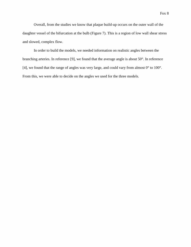
Overall, from the studies we know that plaque build-up occurs on the outer wall of the

daughter vessel of the bifurcation at the bulb (Figure 7). This is a region of low wall shear stress

and slowed, complex flow.

In order to build the models, we needed information on realistic angles between the

branching arteries. In reference [9], we found that the average angle is about 50°. In reference

[4], we found that the range of angles was very large, and could vary from almost 0° to 100°.

From this, we were able to decide on the angles we used for the three models.

Fox 9

IV. METHOD

In this section, I will first discuss the main components involved in our study. This

includes shear stress, turbulence intensity, and turbulence kinetic energy, which were the three

measures we got data about in the simulations, as well as the properties of blood, which were

used to establish a simulation material. Then I will explain the process of the models and

simulations. For this, we had to figure out what governing equations would be appropriate, build

the bifurcation models, use what we learned from the properties of blood, including the

characteristic of pulsatile flow, to determine boundary conditions for the simulations, and

determine an appropriate simulation program.

A) Shear Stress

Stress measures the strength of a material when a force is applied to it. It is the force per

unit area within materials that arises from externally applied forces. Shear stress, denoted by τ, is

the component of stress that is coplanar with a material cross section; the force vector is parallel

to the cross section. Shear stress is the opposite of normal stress, where the force vector is

perpendicular to the material cross section. The general formula for shear stress is

[1]

where is the force applied and is the cross-sectional area. Shear stress is measured in

Newtons per meter squared (N/m2), or Pascals.

Fox 10

i) Shear Stress in Fluids

A fluid is a material that changes shape when a force is applied to it. It does not support

shear stress, so a fluid at rest has zero shear stress and takes the shape of its container. Any fluid

that has a velocity and is moving along a boundary will impress a shear stress on the boundary.

For Newtonian fluids in laminar (streamline) flow, the shear stress is proportional to the strain

rate. Strain is the measure of deformation of a material due to an externally applied force, and the

strain rate is the rate of change in the strain. The constant of proportionality in this relation is the

viscosity of the fluid. Viscosity is the measure of a fluid's resistance to flow. The equation for

shear stress in fluids is

[2]

where is the viscosity, is the velocity of the fluid parallel to the boundary, and is the height

above the boundary. So here, shear stress is a function of the height and is proportional to

viscosity and the velocity gradient. One fluid dynamics principle, the no-slip condition, is that at

the boundary, the speed of the flow will be zero. At some height from the boundary, the flow

will equal the velocity of the fluid. The area in between is the boundary layer. The shear stress on

the boundary is due to this loss of velocity. For non-Newtonian fluids, the shear stress is not

proportional to the strain rate because the fluid viscosity is not constant.

ii) Wall Shear Stress

Wall shear stress is the integral over the wall of shear stress. The equation is

[3]

where τ(y) is given in equation [2]. In this study, we used one material in the simulations, so we

have a given viscosity. The higher the wall shear stress is, the less of a chance there is of plaque

Fox 11

build- up, because there will be a higher velocity gradient, which will detach plaque and carry it

away.

B) Turbulence Intensity and Turbulence Kinetic Energy

A turbulent flow is a flow that has chaotic and non-deterministic property changes. It is

the opposite of laminar flow. Turbulent eddies, or irregular swirls of motions, create fluctuations

in velocity. Turbulence kinetic energy is the mean kinetic energy per unit mass associated with

eddies in a turbulent flow, or the strength of the turbulence in the flow. Kinetic energy is given

by

, where m is mass and v is velocity. Turbulence kinetic energy is similar to

kinetic energy, but since turbulence kinetic energy is measured per unit mass, it corresponds to

. The equation for turbulence kinetic energy is

[4]

or the sum of the average velocity variances divided by two. The total kinetic energy of the flow

is the sum of the kinetic energy of the mean flow and the turbulent flow, . Turbulent

motions associated with eddies are approximately random, so they can be characterized using

statistical concepts. Turbulence intensity is a scale expressing turbulence as a percent. Flow with

no fluctuations would have a turbulence intensity of 0%. Turbulence intensity is defined as

[5]

where u' is the standard deviation of the turbulent velocity fluctuations and U is the mean

velocity of the flow. The higher the turbulence intensity, the higher the level of mixing in the

flow, so there is less of a chance of plaque build-up. Shear stress generates turbulence. The

Fox 12

stronger the shear stress, the stronger the turbulence. This is because the no-slip condition applies

to turbulent velocities as well as the mean flow velocity.

C) Blood Properties and the Simulation Material

A fluid is Newtonian if the strain rate and shear stress are proportional, with the

proportionality constant being the viscosity of the fluid. That is, the viscosity of the fluid does

not depend on the stress state and velocity of the flow. No fluid is perfectly Newtonian, but many

fluids can be assumed to be Newtonian, such as water. A non-Newtonian fluid is simply a fluid

that differs from Newtonian properties, but mainly it is a fluid that has viscosity that is dependent

on the stress state and velocity of the flow. Blood is a non-Newtonian fluid because of the

mixture of cells, proteins, lipoproteins, and ions in the fluid. Some of these substances are

semisolid particles and thereby increase the viscosity of blood. The material we used for this

study is a fluid that has properties between water and blood. It is a Newtonian fluid, like water,

since Newtonian fluids are much easier to simulate. But it has the viscosity and density of blood,

which gives more accurate and realistic results than water. Blood has a viscosity that is about

four times the viscosity of water, but the viscosity is not constant at all flow rates. The Reynolds

number (Re) is the ratio of inertial forces to viscous forces in fluids. For blood flow, Re ranges

from 1 in small arterioles to 4000 in the largest arteries. This range represents flow where

viscous forces are dominant to flow where inertial forces are dominant. In normal pipe flow,

turbulence starts around Re = 2300. Usually, blood flow is around 1000. But the geometry of

blood vessels, among other factors, makes flow turbulent.

Fox 13

D) Governing Equations

Navier-Stokes equations, derived from Newton's second law of momentum conservation

applied to fluid motion, describe the motion of fluids. The equations are nonlinear partial

differential equations. The general form of the equations of fluid motion is

[6]

where v is the flow velocity, ρ is the fluid density, p is the pressure, T is the deviatoric

component of the total stress tensor, and f is the body forces per unit volume acting on the fluid.

The left side of equation [6] describes inertia (

is the unsteady acceleration and is the

convective acceleration) and the right side is a summation of body forces and divergence of

pressure and stress. The del operator, , denotes the gradient of a vector field. The del operator is

defined as

[7]

where , , and are the unit vectors in their respective directions. The equations dictate

velocity rather than position, so a solution is called a velocity field. It describes the velocity of

the fluid at a given point in space and time. The total stress tensor is a tensor, or linear map, that

describes the state of stress at a point inside a material. So the stress tensor T takes a direction

vector as the input and produces the stress on the surface normal to the vector as the output.

Compressibility is a measure of the relative volume change as a response to pressure;

density depends on pressure. Incompressible flow is a flow in which the material density is

constant within an infinitesimal volume that moves with the velocity of the fluid. When

considering an incompressible flow of a Newtonian fluid, the general Navier-Stokes equations

can be simplified since density cancels out. The Navier-Stokes equations for incompressible flow

is

Fox 14

[8]

where f still represents the body forces (this includes gravity, which has an effect on blood flow),

and µ is viscosity. In the simulations of this study, the Navier-Stokes equations for

incompressible flow were used because blood is liquid and will not compress much.

E) Models

Recall from Section III that the average angle of the carotid bifurcation is around 50º and

has a broad range. Therefore, we chose 50º as the average angle model, 70º as the wide angle

model, and 30º as the narrow angle model. The actual values of the models were 50.61º, 70.13º,

and 31.44º, respectively (Figures 1-3). Due to the way the models were built and the angles

adjusted, it was nearly impossible to get the angle to be an exact number. To change the angle,

we had to move points in the plane with the mouse. A seemingly slight move could result in a

drastic change. These values were as close as we could get to the values we wanted.

We built the models using the software SolidWorks. We first built the wide angle model,

then adjusted the angle of it to get the other two models. The first step in constructing the model

was to create the path of the artery. Since the path is not flat, we had to conduct the construction

in a three-dimensional sketch. The path is not straight, so we used a spline tool. To aid the spline

function, we built a box to give references for the spline points. After the spline was placed, the

spline handles were used to define the right curvature of the artery. The same technique was used

to create the branching artery, except the existing spline was also used as a reference point. Next,

points were placed along the splines for future placement of the cross sections. Planes were

constructed at each of these points that were perpendicular to the spline. Then circular cross

sections were created in each plane. The diameter of each cross section was adjusted because the

Fox 15

artery does not have a uniform diameter throughout. The cross sections were then connected

using surface lofts. Because this step was done separately for the main artery and the branched

artery, the section where the surfaces met needed to be trimmed. Then a fillet was added at the

junction to give a smooth transition between the branched artery and the main artery. The last

step was to thicken the walls of the artery so it would be a solid body.

Because geometry-based analysis techniques require that the geometry be broken up into

a discrete representation, we had to produce meshes for the models before we could run the

models through the flow simulation (Figures 4-6). For the simulations, we took a cross section of

each model at the daughter vessel, close to the bifurcation (Figures 8-9). We measured the wall

shear stress, turbulence intensity, and turbulence kinetic energy of the flow through the cross

sections.

F) Pulsatile Flow

The heart pumps blood through the cardiovascular network in a cyclic nature, creating a

pulsatile flow, where flow velocity and pressure are unsteady. Blood is pumped out of the heart

during systole and rests during diastole. In some arteries, such as the carotid bifurcation, blood

flow can be reversed during diastole, when the pressure is zero or close to zero. In the flow

simulations, we ran the simulations twice for each model and measure, one with up flow and one

with down flow to account for this reversal of flow. Figure 28 shows modeled blood flow

through the carotid bifurcation. A unique feature of the carotid bifurcation is the bulb at the

beginning of the internal carotid artery. "The main stream moves upward along the centerline

and flow divider along the posterior wall... counter-rotating secondary vortices move upstream

toward the common carotid in a separation region," [8]. This upstream movement toward the

Fox 16

common carotid is the reversal of flow during diastole. It is on the outer wall of the bulb where

the reversal occurs, contributing to the flow velocity fluctuations and low shear stress in this

area.

G) Boundary Conditions

For the simulation, we needed boundary conditions to solve the Navier-Stokes equations.

These boundaries help direct the motion of flow, and describe the entrance and exit of the flow.

One boundary condition we used was the no-slip condition, where the velocity of the flow is zero

at the wall of the blood vessel. For the inlet conditions, we had a constant mass flow rate based

on the peaks of the pulsatile flow data from reference [9], we set the turbulence intensity,

pressure was calculated, and we had a fully developed velocity profile. For the outlet conditions,

the pressure was calculated, and we had zero diffusion flux and overall mass balance. The last

two outlet conditions are set to make sure that the amount of fluid going through the simulation

is the same going in the vessel and coming out of the vessel. Since the flow is pulsatile, we

extracted input flow rate points from a table in [9], and fitted a formula to them using Matlab.

For the curve fit, a 4-term Fourier fit was used. Figure 29 is an image of the fitted curve. On the

curve, there is a main maximum and a main minimum. These correspond to the up flow and

down flow, respectively, discussed in Section H.

H) Flow Simulation

Once the models were built and the boundary conditions were set, the flow simulations

could be run. In the simulation, the program used was a Navier-Stokes solver with K-Omega

turbulence modeling. The K-Omega model is a two-equation model that represents the turbulent

Fox 17

properties of flow. It determines the scale and energy of the turbulence. The simulation used the

SIMPLE algorithm as the Navier-Stokes solver, and coupled pressure and velocity. SIMPLE

stands for Semi-Implicit Method for Pressure Linked Equations. According to [12], the basic

steps of the algorithm are:

"1. Set the boundary conditions.

2. Compute the gradients of velocity and pressure.

3. Solve the discretized momentum equation to compute the intermediate velocity field.

4. Compute the uncorrected mass fluxes at faces.

5. Solve the pressure correction equation to produce cell values of the pressure correction.

6. Update the pressure field.

7. Update the boundary pressure corrections.

8. Correct the face mass fluxes.

9. Correct the cell velocities.

10. Update density due to pressure changes."

The algorithm is iterative. "An approximation of the velocity field is obtained by solving the

momentum equation. The pressure gradient term is calculated using the pressure distribution

from the previous iteration or an initial guess. The pressure equation is formulated and solved in

order to obtain the new pressure distribution. Velocities are corrected and a new set of

conservative fluxes is calculated [12]."

Fox 18

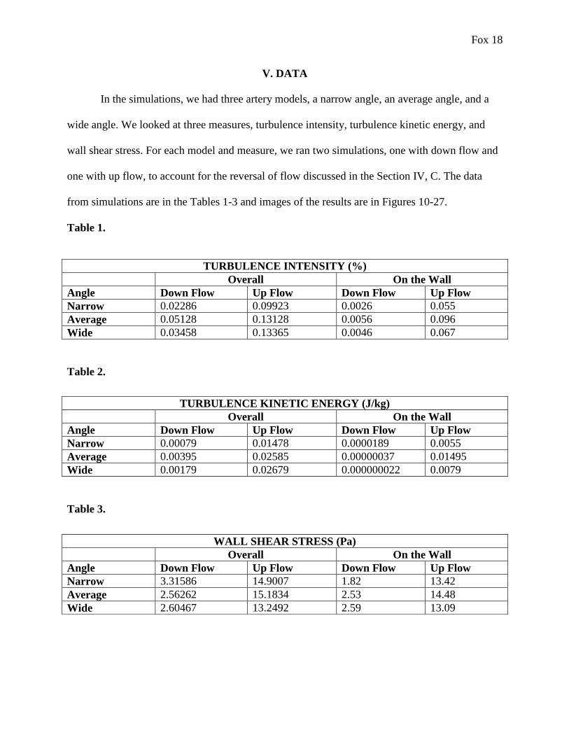
V. DATA

In the simulations, we had three artery models, a narrow angle, an average angle, and a

wide angle. We looked at three measures, turbulence intensity, turbulence kinetic energy, and

wall shear stress. For each model and measure, we ran two simulations, one with down flow and

one with up flow, to account for the reversal of flow discussed in the Section IV, C. The data

from simulations are in the Tables 1-3 and images of the results are in Figures 10-27.

Table 1.

Table 2.

Table 3.

TURBULENCE INTENSITY (%)

Overall On the Wall

Angle Down Flow Up Flow Down Flow Up Flow

Narrow 0.02286 0.09923 0.0026 0.055

Average 0.05128 0.13128 0.0056 0.096

Wide 0.03458 0.13365 0.0046 0.067

TURBULENCE KINETIC ENERGY (J/kg)

Overall On the Wall


Narrow 0.00079 0.01478 0.0000189 0.0055

Average 0.00395 0.02585 0.00000037 0.01495

Wide 0.00179 0.02679 0.000000022 0.0079

WALL SHEAR STRESS (Pa)

Overall On the Wall


Narrow 3.31586 14.9007 1.82 13.42

Average 2.56262 15.1834 2.53 14.48

Wide 2.60467 13.2492 2.59 13.09

Fox 19

In our analysis of the data, there were two main considerations. One involved the up flow and

down flow simulations. Since up flow is what mostly occurs in the carotid artery (arteries move

blood away from the heart, which would be in an up direction, toward the head, in the carotid

arteries) and down flow represents the reversal of flow, we considered the up flow simulations as

the more important outcomes. The up flow results also showed a more drastic change between

the models. The second consideration involved was where in the cross section of the artery the

data came from. It was important to this study to not just consider the data from the overall cross

section, but the data that came from the wall of the cross section, since this is where plaque

build-up occurs.

When the wall and the up flow is taken into consideration, the highest values for all three

measures occurs in the average angle model. The lowest values of turbulence intensity and

turbulence kinetic energy occurs in the narrow angle model, and the lowest value of the wall

shear stress occurs in the wide angle model. Figures 30-38 are images of the wall of the cross

sections for each of the measures in the up flow simulations. Tables 4-9 show the percent

difference between each model for each measure.

Table 4.

Percent Difference, Turbulence Intensity, Up Flow, Overall

Narrow Angle Average Angle

Narrow Angle --- ---

Average Angle 27.81% ---

Wide Angle 29.56% 1.79%

Table 5.

Percent Difference, Turbulence Intensity, Up Flow, On the Wall




Wide Angle 19.67% 35.58%

Fox 20

Table 6.

Percent Difference, Turbulence Kinetic Energy, Up Flow, Overall




Wide Angle 57.78% 3.57%

Table 7.

Percent Difference, Turbulence Kinetic Energy, Up Flow, On the Wall




Wide Angle 35.82% 61.71%

Table 8.

Percent Difference, Wall Shear Stress, Up Flow, Overall




Wide Angle 11.73% 13.61%

Table 9.

Percent Difference, Wall Shear Stress, Up Flow, On the Wall




Wide Angle 2.49% 10.08%

Fox 21

VI. CONCLUSIONS

When we first started this study, we hypothesized that the narrower the angle between the

branching arteries, the higher the turbulence intensity, turbulence kinetic energy, and wall shear

stress, and thus the lower the chance of atherosclerosis. The first two simulations we ran were on

the wide angle and average angle models. The data from these two simulations led us to believe

that our hypothesis was correct. However, when the data came back from the simulation on the

narrow angle model, it was clear that our hypothesis needed to be revised. The highest values of

all three measures occurred in the average angle model, indicating that the least chance of

atherosclerosis occurs when the branching arteries are about 50° apart. This means that instead

the lowest angle being best, there is an optimal angle at which the three measures are highest.

Fox 22

VII. DISCUSSION

The end goal of our study is to enhance current knowledge of cardiovascular disease.

Ultimately, doctors would be able to look at images of the carotid arteries, or other blood vessels,

from MRIs and other imaging devices, and determine if a patient is at risk for heart disease. With

this knowledge of potential risk, a patient could modify diet and lifestyle to counteract this risk

factor. If a doctor had this capability, deaths from cardiovascular disease could be decreased.

The next step in this study would be to find the exact optimal angle. This might require a

different construction method for the models so that the exact angle could be entered. We are

continuing the study on the theoretical reason behind the existence of an optimal angle, instead

of the lowest angle being best. There would have to be something about a narrower angle that

slows the flow or obstructs the unidirectional, streamline flow. We are currently working to

figure this out. Also, the data from the narrow angle simulation could be misleading. The cross

section from the narrow angle model actually extended into the main vessel a bit. (This is the

reason why the images of the results of the narrow angle model are not circular.)

Further work that could be done with this project would include using a more accurate

and realistic material that has more similar properties to blood. One of these properties to

consider would be a material that is non-Newtonian. We chose to use a Newtonian material

because it is good for qualitative comparisons, which was the intended outcome of this study,

rather than exact quantitative results. Also, if we had used a non-Newtonian material, we would

not have been able to use the K-Omega model and the simulations would have taken more

computing time. Another property to consider would be the elastic property of vessels. Other

aspects of the vessel geometry could be tested as well, such as the cross sectional shape of the

Fox 23

vessel. In our models, the cross sections were circular. Other measures of fluid dynamics besides

shear stress, turbulence intensity, and turbulence kinetic energy could be tested in the flow

simulations too. Overall, future work on this project would involve making the models and

simulation more life-like.

Fox 24

VIII. REFERENCES

[1] "The Arteries of the Head and Neck: The Common Carotid Artery." Human Anatomy. N.p.,

n.d. Web. 1 Dec. 2012. <http://www.theodora.com/anatomy/the_common_carotid_artery.html>.

[2] Asakura, T., and T. Karino. "Flow Patterns and Spatial Distribution of Atherosclerotic

Lesions in Human Coronary Arteries." Journal of the American Heart Association 66 (1990):

1045-066. Web.

[3] Biomedical Engineering Branched Vein Tutorial. SolidWorks, 2012. YouTube.

[4] Fisher, M., and S. Fieman. "Geometric Factors of the Bifurcation in Carotid Atherogenesis."

Journal of the American Heart Association: Stroke 21 (1990): 267-71. American Heart

Association. Web. 15 Mar. 2013. <http://stroke.ahajournals.org/content/21/2/267.full.pdf>.

[5] "Geometry of Blood Vessels May Influence Heart Disease." ScienceDaily. N.p., 4 Sept.

1998. Web. <http://www.sciencedaily.com/releases/1998/09/980904035915.htm>.

[6] "Heart Disease: Scope and Impact." The Heart Foundation. N.p., 2012. Web. 1 Dec. 2012.

<http://www.theheartfoundation.org/heart-disease-facts/heart-disease-statistics/>.

[7] Huo, Yunlong, and Ghassan S. Kassab. "Pulsatile Blood Flow in the Entire Coronary Arterial

Tree: Theory and Experiment." AJP- Heart and Circulatory Physiology 291 (2006): H1074-

1087. Web.

[8] Ku, David N. "Blood Flow in Arties." Annual Reviews, Fluid Mechanics 29 (1997): 399-434.

Annual Reviews Inc. Web. 29 Apr. 2013.

[9] Ku, D. N., D. P. Giddens, C. K. Zarins, and S. Glagov. "Pulsatile Flow and Atherosclerosis in

the Human Carotid Bifurcation, Positive Correlation Between Plaque Location and Low

Oscillating Shear Stress." Journal of the American Heart Association 5 (1985): 293-302. Web.

[10] Lee, D., and J. J. Chiu. "Intimal Thickening Under Shear in a Carotid Bifurcation- A

Numerical Study." Journal of Biomechanics 29.1 (1996): 1-11. Elsevier Science Ltd. Web. [11] Rieutord, Thibault. Navier-Stokes 1D Model for Blood Flow Simulations in a Vascular

Network. Tech. N.p.: n.p., n.d. Print.

[12] "SIMPLE [Semi-Implicit Method for Pressure-Linked Equations]." CFD Online. N.p., 28

Dec. 2011. Web. 29 Apr. 2013. <http://www.cfd-online.com/Wiki/SIMPLE_algorithm>.

[13] Urquiza, Santiago, Pablo Blanco, Guillermo Lombera, Marcelo Venere, and Raul Feijoo.

"Coupling Multidimensional Compliant Models for Carotid Artery Blood Flow." Mecanica

Computacional XXII (2003): n. pag. Web.

Fox 25

[14] "What Causes a Heart Attack?" National Heart Lung and Blood Institute. National Institutes

of Health, 1 Mar. 2011. Web. 1 Dec. 2012. <http://www.nhlbi.nih.gov/health/health-

topics/topics/heartattack/causes.html>.

[15] "What Is Atherosclerosis?" WebMD. WebMD, n.d. Web. 1 Dec. 2012.

<http://www.webmd.com/heart-disease/what-is-atherosclerosis>.

[16] Zarins, C. K., D. P. Giddens, B. K. Bharadvaj, V. S. Sottiurai, R. F. Mabon, and S. Glagov.

"Carotid Bifurcation Atherosclerosis, Quantitative Correlation of Plaque Localization with Flow

Velocity Profiles and Wall Shear Stress." Journal of the American Heart Association 1983.53

(1983): 502-14. Web.

Fox 26

IX. FIGURES

Figure 4. Example of the mesh

Figure 5.

Example of the mesh

Figure 6. Example of the mesh

Figure 1.

Narrow angle model Figure 2.

Average angle model Figure 3.

Wide angle model

Fox 27

Figure 7. Outer wall of the daughter vessel at the bulb

Figure 8.

Cross section Figure 9.

Cross section

Fox 28

Figure 10.

Cross section of results, turbulence intensity,

narrow angle, down flow

Figure 11.


narrow angle, up flow

Figure 12.


average angle, down flow

Figure 13.


average angle, up flow

Figure 14.


wide angle, down flow

Figure 15.


wide angle, up flow

Fox 29

Figure 16.

Cross section of results, turbulence kinetic

energy, narrow angle, down flow

Figure 17.


energy, narrow angle, up flow

Figure 18.


energy, average angle, down flow

Figure 19.


energy, average angle, up flow

Figure 20.


energy, wide angle, down flow

Figure 21.


energy, wide angle, up flow

Fox 30

Figure 22.

Cross section of results, wall shear stress,

narrow angle, down flow

Figure 23.



Figure 24.


average angle, down flow

Figure 25.



Figure 26.

Cross section of results, wall shear stress, wide

angle, down flow

Figure 27.

Cross section of results, wall shear stress, wide

angle, up flow

Fox 31

Figure 28. Modeled flow in the carotid artery bifurcation

Figure 29. Fourier fit curve for input flow rate.

Fox 32

Figure 30.

Close up of wall of cross

section, turbulence intensity,


Figure 31.




Figure 32.



wide angle, up flow

Figure 33.


section, turbulence kinetic

energy, narrow angle, up flow

Figure 34.



energy, average angle, up

flow

Figure 35.



energy, wide angle, up flow

Figure 36.


section, wall shear stress,


Figure 37.


section, wall shear stress,


Figure 38.


section, wall shear stress, wide

angle, up flow

Numerical study of the effect of blood vessel geometry on - faculty

Documents

Transcript of Numerical study of the effect of blood vessel geometry on - faculty