44

Numerical study of high-lift hydrofoil near free surface at moderate Froude number * Tao Xing1, Konstantin I. Matveev2, Miles P. Wheeler2 1. Department of Mechanical Engineering, The University of Idaho, Moscow, Idaho, USA 2. School of Mechanical and Materials Engineering, Washington State University, Pullman, Washington, USA (Received February 21, 2019, Revised September 20, 2019, Accepted September 21, 2019, Published online December 11, 2019) ©China Ship Scientific Research Center 2020 Abstract: Shallow hydrofoils are known to produce lower lift in normal operating conditions in comparison with deep hydrofoils. However, the maximum lift capability of shallow hydrofoils at moderate speeds, which is important for transitional regimes of hydrofoil boats, is studied insufficiently. In this work, two-dimensional flow around a high-lift hydrofoil at a moderate Froude number is numerically simulated in a broad range attack angles up to the stall occurrence in both single-phase fluid and in the vicinity of free surface. It is found that nearly the same maximum lift coefficient can be produced by the shallow foil in the modeled condition as by the deep foil, but much higher attack angle is required near the free surface, which also results in larger drag. Additionally, it is shown that higher Reynolds numbers lead to higher lift coefficients, especially at large attack angles. Key words: Hydrofoil, numerical simulation, free surface effect, stall Introduction

Hydrofoils are some of the most hydrodyna- mically efficient bodies that can generate high lift at low drag when moving through the water. Fast boats equipped hydrofoils can elevate their hulls so that the hull’s water drag becomes small, thus allowing these boats to achieve high speeds. Hydrofoil ships were developed and widely used in the second half of the last century for passenger transportation[1]. Their typical speeds and capacities are around 30 kn-40 kn and 100-250 passengers, respectively. However, in case of heavy-payload requirements these boats are not so efficient, and other types of marine craft, such as large multi-hulls, proved to be more suitable for combined passenger/car transportation, especially when the intended relative speeds (Froude numbers) are lower. Hydrofoil profiles used in common surface-piercing foil systems are usually thin and often have flat lower surfaces (Fig. 1(a)). Although such shapes are not the most efficient for single-phase flows, their characteristics at high speeds in water are adequate, and these low-profile sections are less

* Biography: Tao Xing (1973-), Male, Ph. D., P. E., Associate Professor Corresponding author: Tao Xing, E-mail: xing@uidaho.edu

susceptible to air ventilation, when suction of the atmospheric air to the lifting foil surface reduces the generated lift[2]. These hydrofoils are also beneficial for delaying cavitation to higher speeds. At lower speed, however, thin low-camber profiles cannot produce enough lift, which leads to higher operational speeds that require much greater propulsion power.

Thicker, more cambered airfoil-type sections, such as shown in Fig. 1(b), can potentially produce higher lift and increase lift-drag ratio at lower speeds and thus reduce operational speeds (or Froude numbers) at which hydrofoils can still be beneficial. This can help foil-assisted boats be more economical at higher payloads and/or lower speeds. In principle, the air ventilation problem can be mitigated with application of fences or other techniques[3-4]. Although such hydrofoils would be prone to cavitation at high speeds, in case of relatively low operational speeds the cavitation is not an issue. Another hydrodynamic consideration important for hydrofoils operating near a free surface is the effect of the shallow submergence on the occurrence of stall and specifically on the maximum lift coefficient of the foil, which is a vital property for elevating the boat hull out of water and overcoming the boat hump drag.

It is well known that lift of hydrofoils generally recedes with approaching the free surface at moderate attack angles and typical speeds[5]. However, accor-

Available online at https://link.springer.com/journal/42241 http://www.jhydrodynamics.com

Journal of Hydrodynamics, 2020, 32(1): 44-53 https://doi.org/10.1007/s42241-019-0095-0

45

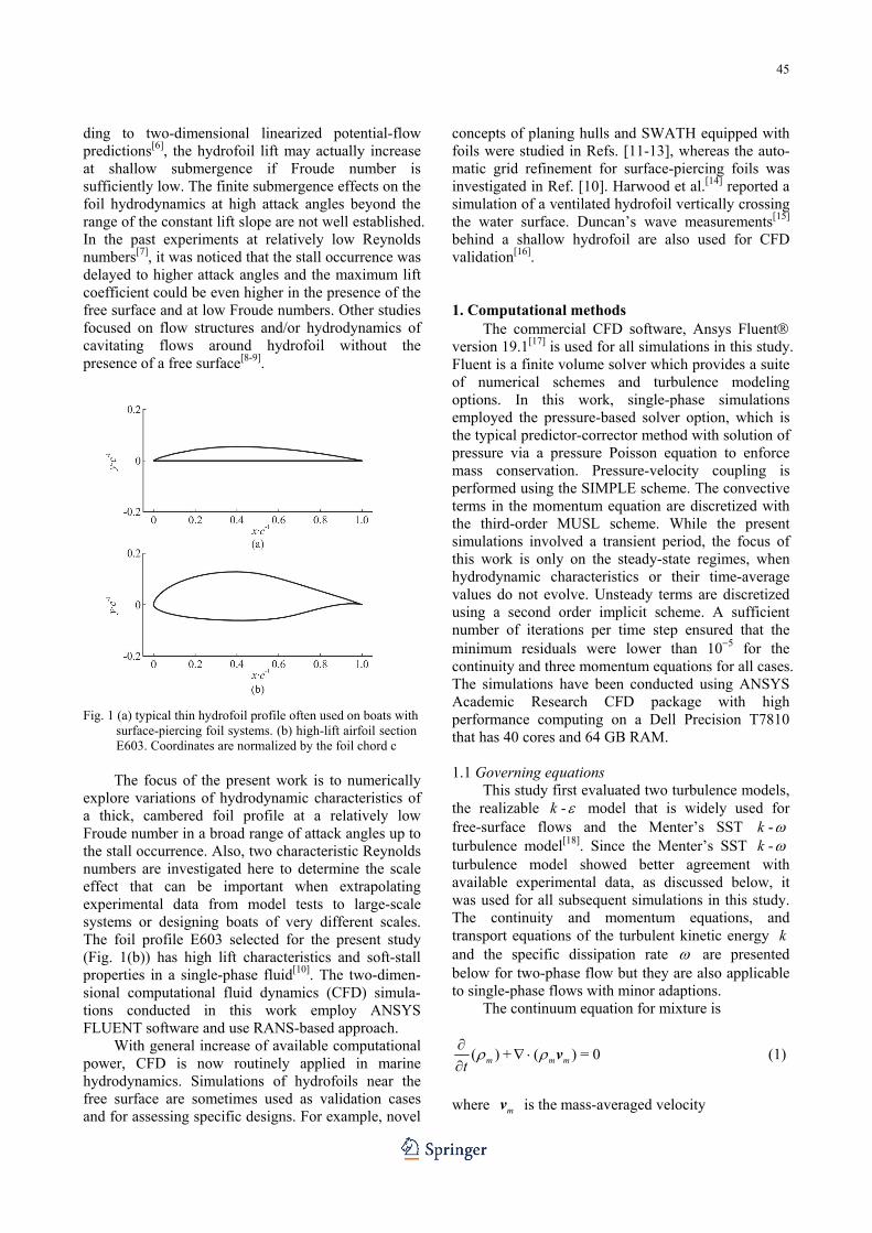
ding to two-dimensional linearized potential-flow predictions[6], the hydrofoil lift may actually increase at shallow submergence if Froude number is sufficiently low. The finite submergence effects on the foil hydrodynamics at high attack angles beyond the range of the constant lift slope are not well established. In the past experiments at relatively low Reynolds numbers[7], it was noticed that the stall occurrence was delayed to higher attack angles and the maximum lift coefficient could be even higher in the presence of the free surface and at low Froude numbers. Other studies focused on flow structures and/or hydrodynamics of cavitating flows around hydrofoil without the presence of a free surface[8-9]. Fig. 1 (a) typical thin hydrofoil profile often used on boats with surface-piercing foil systems. (b) high-lift airfoil section E603. Coordinates are normalized by the foil chord c The focus of the present work is to numerically explore variations of hydrodynamic characteristics of a thick, cambered foil profile at a relatively low Froude number in a broad range of attack angles up to the stall occurrence. Also, two characteristic Reynolds numbers are investigated here to determine the scale effect that can be important when extrapolating experimental data from model tests to large-scale systems or designing boats of very different scales. The foil profile E603 selected for the present study (Fig. 1(b)) has high lift characteristics and soft-stall properties in a single-phase fluid[10]. The two-dimen- sional computational fluid dynamics (CFD) simula- tions conducted in this work employ ANSYS FLUENT software and use RANS-based approach. With general increase of available computational power, CFD is now routinely applied in marine hydrodynamics. Simulations of hydrofoils near the free surface are sometimes used as validation cases and for assessing specific designs. For example, novel

concepts of planing hulls and SWATH equipped with foils were studied in Refs. [11-13], whereas the auto- matic grid refinement for surface-piercing foils was investigated in Ref. [10]. Harwood et al.[14] reported a simulation of a ventilated hydrofoil vertically crossing the water surface. Duncan’s wave measurements[15] behind a shallow hydrofoil are also used for CFD validation[16]. 1. Computational methods The commercial CFD software, Ansys Fluent version 19.1[17] is used for all simulations in this study. Fluent is a finite volume solver which provides a suite of numerical schemes and turbulence modeling options. In this work, single-phase simulations employed the pressure-based solver option, which is the typical predictor-corrector method with solution of pressure via a pressure Poisson equation to enforce mass conservation. Pressure-velocity coupling is performed using the SIMPLE scheme. The convective terms in the momentum equation are discretized with the third-order MUSL scheme. While the present simulations involved a transient period, the focus of this work is only on the steady-state regimes, when hydrodynamic characteristics or their time-average values do not evolve. Unsteady terms are discretized using a second order implicit scheme. A sufficient number of iterations per time step ensured that the minimum residuals were lower than 105 for the continuity and three momentum equations for all cases. The simulations have been conducted using ANSYS Academic Research CFD package with high performance computing on a Dell Precision T7810 that has 40 cores and 64 GB RAM. 1.1 Governing equations This study first evaluated two turbulence models, the realizable -k model that is widely used for free-surface flows and the Menter’s SST -k turbulence model[18]. Since the Menter’s SST -k turbulence model showed better agreement with available experimental data, as discussed below, it was used for all subsequent simulations in this study. The continuity and momentum equations, and transport equations of the turbulent kinetic energy k and the specific dissipation rate are presented below for two-phase flow but they are also applicable to single-phase flows with minor adaptions. The continuum equation for mixture is

( ) + ( ) = 0m m mt

v

(1)

where mv is the mass-averaged velocity

46

=1=

n

k k kkm

m

vv

(2)

and m is the mixture density

=1

=n

m k kk

(3)

where k is the volume fraction of phase k , n is

the number of phases. The equation for the conservation of momentum can be written as

T+ ( ) = + [ ( + )] +

m m

m m m m m mpt

vv v v v

+mg F

(4)

where p is the gage pressure, F is a body force,

g is the gravitational acceleration and m is the

viscosity of the mixture

=1

=n

m k kk

(5)

Governing equations for the Menter’s SST -k turbulence model:

( ) + ( ) = + +

tm m m m

k

k k kt

v

+k k kG Y S

(6)

( ) + ( ) = + +

t

m m m mtv

+ + G Y D S

(7)

where kS and S are user-defined source terms.

1 ,1 1 , 2

1=

/ + (1 ) /kk kF F

(8)

1 ,1 1 ,2

1=

/ + (1 ) /F F

(9)

Model constants are ,1 = 1.176k , ,1 = 2 , ,2 = 1k

and ,2 = 1.168 . The blending function 1F is

given by

41 1= tanh( )F

(10)

1 2 + 2,2

500 4= min max , ,

0.09

k k

y y D y

(11)

+ 10

,2

1 1= max 2 ,10

j j

kD

x x

(12)

where y is the distance to the next surface, +D is

the positive portion of the cross-diffusion term

2*

1

1=

1max ,

t

k

SF

(13)

where S is the strain rate magnitude, * damps the turbulent viscosity causing a low-Reynolds number correction:

+ +j ji i

j i j i

u uu uS

x x x x

(14)

*

* * 0 + /=

1+ /t k

t k

Re R

Re R

(15)

=t

kRe

, = 6kR , *0 = 0.024

(16)

2

2 2= tanh( )F

(17)

2 2

500= max 2 ,

0.09

k

y y

(18)

In these equations, the term kG and G repre-

sent the production of turbulence kinetic energy k and generation of , respectively.

2=k tG S

(19)

2= =kt

G G S

(20)

*=kY k

(21)

47

2= iY

(22)

1 ,1 1 ,2= + (1 )i i iF F

(23)

1 ,2

1= 2(1 )

j j

kD F

x x

(24)

where * = 0.09 , ,1 = 0.075i , ,2 = 0.0828i .

The tracking of the interface between the phases is accomplished by solving the continuity equation for the volume fraction of one of the phases. For thq

phase, this equation is

=1

1( ) + ( ) = ( )

n

q q q q q pq qppq

m mt

v

(25)

where qpm is the mass transfer from phase q to

phase p , pqm is the mass transfer from phase p

to phase q . The volume fraction equation will not be

solved for the primary phase, the primary-phase volume fraction is computed based on the following

=1

= 1n

qq

(26)

The two most important hydrodynamic characte- ristics of hydrofoil performance, the lift and drag coefficients, are used for presenting results in the next sections. These metrics are defined as follows:

2=

0.5L

LC

U c

(27)

2=

0.5D

DC

U c

(28)

where L and D are the lift and drag forces, U is the incident flow velocity and c is the foil chord.

The variable input parameters include the foil submer- gence and Reynolds and Froude numbers:

=Uc

Re

(29)

=U

Frgc

(30)

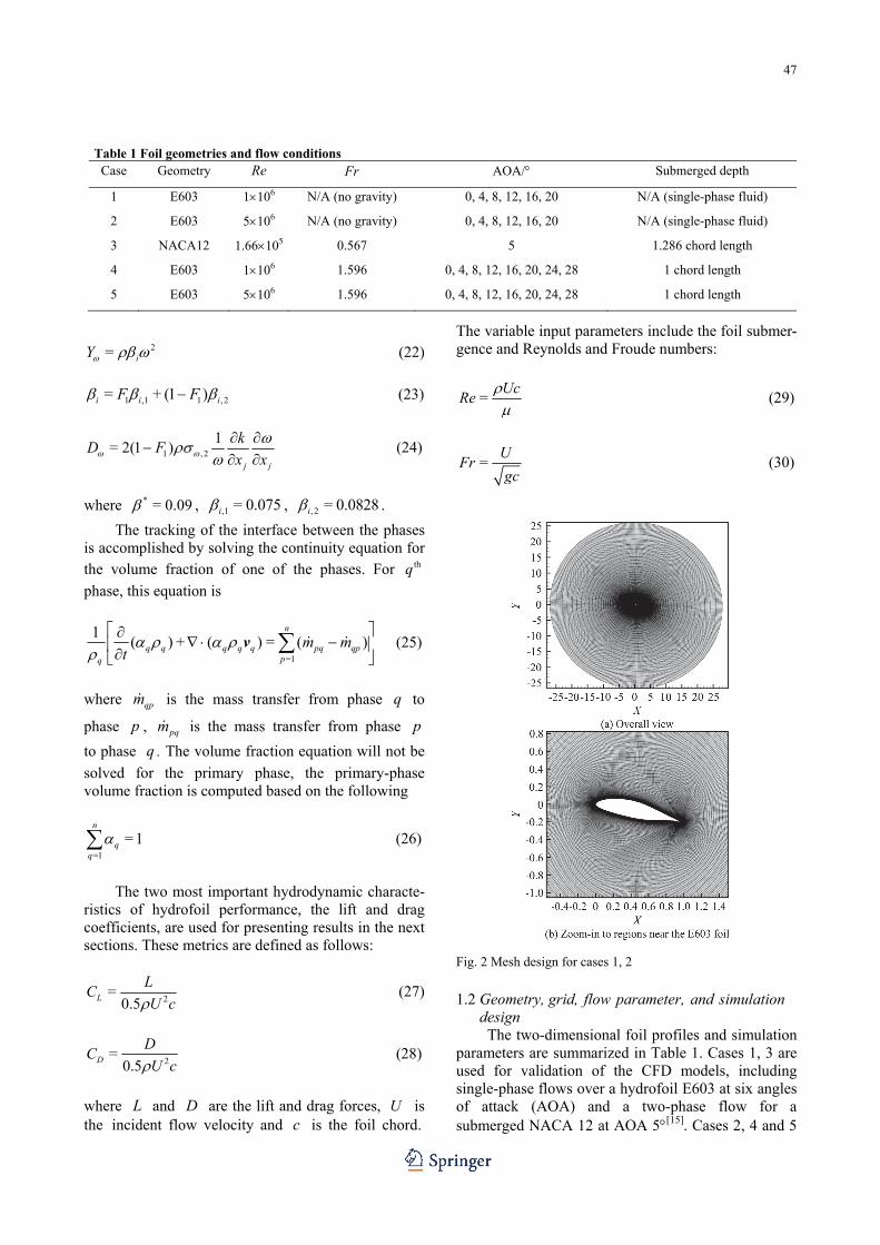
Fig. 2 Mesh design for cases 1, 2 1.2 Geometry, grid, flow parameter, and simulation design The two-dimensional foil profiles and simulation parameters are summarized in Table 1. Cases 1, 3 are used for validation of the CFD models, including single-phase flows over a hydrofoil E603 at six angles of attack (AOA) and a two-phase flow for a submerged NACA 12 at AOA 5[15]. Cases 2, 4 and 5

Table 1 Foil geometries and flow conditions Case Geometry Re Fr AOA/ Submerged depth

1 E603 1106 N/A (no gravity) 0, 4, 8, 12, 16, 20 N/A (single-phase fluid)

2 E603 5106 N/A (no gravity) 0, 4, 8, 12, 16, 20 N/A (single-phase fluid)

3 NACA12 1.66105 0.567 5 1.286 chord length

4 E603 1106 1.596 0, 4, 8, 12, 16, 20, 24, 28 1 chord length

5 E603 5106 1.596 0, 4, 8, 12, 16, 20, 24, 28 1 chord length

48

employed the validated CFD models to investigate the effect of AOA, submergence and Re on the lift and drag coefficients of the high-lift hydrofoil E603. For cases 1, 2, a two-dimensional O-type grid is created to model the flow (Fig. 2). Compared with a C-type grid, the O-type grid has advantages of specifying boundary conditions at any AOAs. The fine grid has a total of 770 788 cells. For solution verification, additional two coarser grids are created systematically using a constant grid refinement ratio

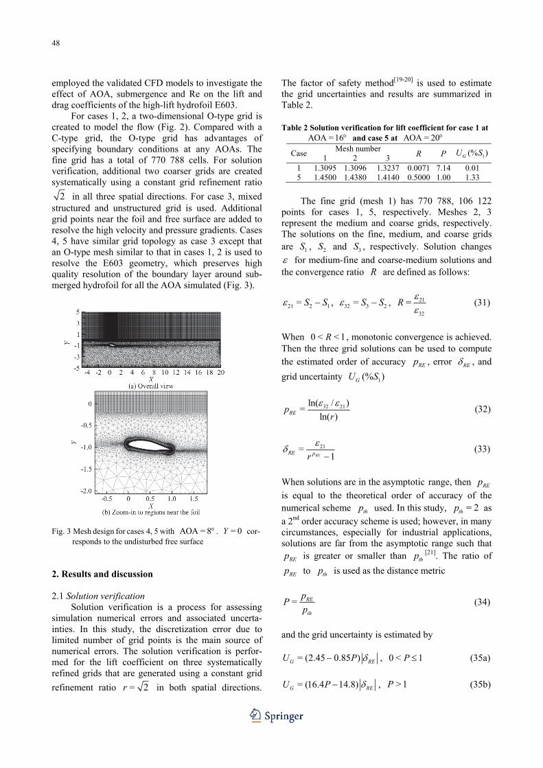
2 in all three spatial directions. For case 3, mixed structured and unstructured grid is used. Additional grid points near the foil and free surface are added to resolve the high velocity and pressure gradients. Cases 4, 5 have similar grid topology as case 3 except that an O-type mesh similar to that in cases 1, 2 is used to resolve the E603 geometry, which preserves high quality resolution of the boundary layer around sub- merged hydrofoil for all the AOA simulated (Fig. 3).

Fig. 3 Mesh design for cases 4, 5 with AOA = 8 . = 0Y cor- responds to the undisturbed free surface 2. Results and discussion 2.1 Solution verification Solution verification is a process for assessing simulation numerical errors and associated uncerta- inties. In this study, the discretization error due to limited number of grid points is the main source of numerical errors. The solution verification is perfor- med for the lift coefficient on three systematically refined grids that are generated using a constant grid

refinement ratio = 2r in both spatial directions.

The factor of safety method[19-20] is used to estimate the grid uncertainties and results are summarized in Table 2. Table 2 Solution verification for lift coefficient for case 1 at AOA =16 and case 5 at AOA = 20

CaseMesh number

R P 1(% )GU S1 2 3

1 1.3095 1.3096 1.3237 0.0071 7.14 0.01 5 1.4500 1.4380 1.4140 0.5000 1.00 1.33

The fine grid (mesh 1) has 770 788, 106 122 points for cases 1, 5, respectively. Meshes 2, 3 represent the medium and coarse grids, respectively. The solutions on the fine, medium, and coarse grids are 1S , 2S and 3S , respectively. Solution changes

for medium-fine and coarse-medium solutions and the convergence ratio R are defined as follows:

21 2 1= S S , 32 3 2= S S , 21

32

=R

(31)

When 0 < < 1R , monotonic convergence is achieved. Then the three grid solutions can be used to compute the estimated order of accuracy REp , error RE , and

grid uncertainty 1(% )GU S

32 21ln( / )

=ln( )REp

r

(32)

21=

1RERE pr

(33)

When solutions are in the asymptotic range, then REp

is equal to the theoretical order of accuracy of the numerical scheme thp used. In this study, = 2thp as

a 2nd order accuracy scheme is used; however, in many circumstances, especially for industrial applications, solutions are far from the asymptotic range such that

REp

is greater or smaller than thp [21]. The ratio of

REp to thp

is used as the distance metric

= RE

th

pP

p

(34)

and the grid uncertainty is estimated by

= (2.45 0.85 )G REU P , 0 < 1P

(35a)

= (16.4 14.8)G REU P , > 1P

(35b)

49

As shown in Table 2, monotonic convergence is achieved for both cases with a low grid uncertainty of

10.01%S and 11.33%S for Cases 1, 5, respectively.

This suggests that the current fine grid resolution is adequate, and this fine grid is used for all simulations. 2.2 Validation for E603 foil in single-phase fluid (case 1) Figure 4 shows the comparison of the lift coefficients obtained with the realizable -k model and the -k SST model against experimental data[22]. Overall, both turbulence models agree reasonably with test data at low attack angles. As one can see in Fig. 4, the -k SST model outperforms

-k model, since it is closer to the test data and also better predicts the stalling regime that was failed to be properly captured using the -k model. Thus, the

-k SST model was adopted for other simulations in this study. Fig. 4 Lift coefficient of E603 foil at various AOA (case 1)

Fig. 5 (Color online) Comparison of wave profile between CFD and experiment for case 3 2.3 Validation of CFD model for submerged NACA 12 (case 2) The CFD model is also validated against experimental data for wave profiles generated by a submerged NACA0012 hydrofoil profile reported in Ref. [15]. In this study, the leading edge of foil was located at = 0x , whereas the chord length of the foil was taken as 0.203 m. The depth of submergence is 1.286c , which is defined as the vertical distance between the free surface and the midpoint of the chord line of the foil. Both the realizable -k model and

the -k SST model were evaluated, but they showed nearly identical results for this case. Therefore, only the result from the -k SST model is presented in Fig. 5. Again, CFD agrees well with experiment, but slightly underpredicts the wave amplitudes. 2.4 Effects of Free surface and Reynolds number Four curves in Fig. 6 represent numerical results obtained for the lift and drag coefficients of E603 hydrofoil under two Reynolds numbers for no-gravity, single-phase situation (cases 1, 2) and for finite- gravity, finite-submergence condition (cases 4, 5). In order to make proper comparison, a correction due to buoyancy has been added to the no-gravity, single- phase lift coefficients. Fig. 6 Lift and drag coefficient of E603 hydrofoil

For the single-phase situations, increase of Re lead to higher magnitudes of LC , especially at large

AOAs near the stall regime (Fig. 6(a)). For the foil under a free surface, the effect of Re on LC is

similar but slightly less pronounced. This observation suggests that model-scale boat hulls having hydrofoils at high AOA (likely in the transition from hull-borne to foil-borne state) would demonstrate inferior lift performance in comparison to full-scale boats. Hence, if a small-scale hull is able to overcome transitional hump drag under given propulsion level, then additional margin will be built up in the design and

50

will likely ensure successful transition to the foil- borne mode of the full-size hydrofoil boat. The effect of finite foil submergence at small AOA is a reduction of the lift slope (Fig. 6(a)), which is well-known phenomenon. However, the maximum

LC is not decreased, it just shifts to higher AOA, thus

delaying stall to higher attack angles. These findings are in agreement with early experimental measure- ments conducted at lower Reynolds numbers[7]. The reduction of the lift slope when approaching the maximum lift condition is more gradual for the foil near a free surface. Hence, if one needs to produce high lift on a hydrofoil (e.g., while the boat transits from hull-borne to foil-borne state), much higher AOA than usual can be employed, since stall is delayed. The effect of Reynolds number on the drag coefficient of a two-dimensional foil is found to be relatively small in the present simulations (Fig. 6(b)). For single-phase situations, higher Re leads to generally lower DC . In cases with the free surface,

drag at different Reynolds numbers is nearly the same at low AOA, while higher Re results in somewhat bigger DC near the stall region. It should be kept in

mind that real finite-span hydrofoils would also have substantial lift-induced drag due to trailing vortices. With regard to the submergence effect on drag, hydrofoils near the free surface naturally have higher

DC due to generation of surface waves.

For single-phase flow cases 1, 2, the gravity force is excluded. Therefore, pressure coefficient is used for analysis

ref2

=0.5p

p pC

U

(36)

where p is the gage pressure on the foil surface,

refp is the reference gage pressure at inlet/far- field.

For two-phase flow cases 4, 5, the gravity force must be included in the simulations due to the presence of a free surface. In that case, piezometric pressure coefficient is used

2

+=

0.5p

p zC

U

(37)

where is the specific weight of water, z is the

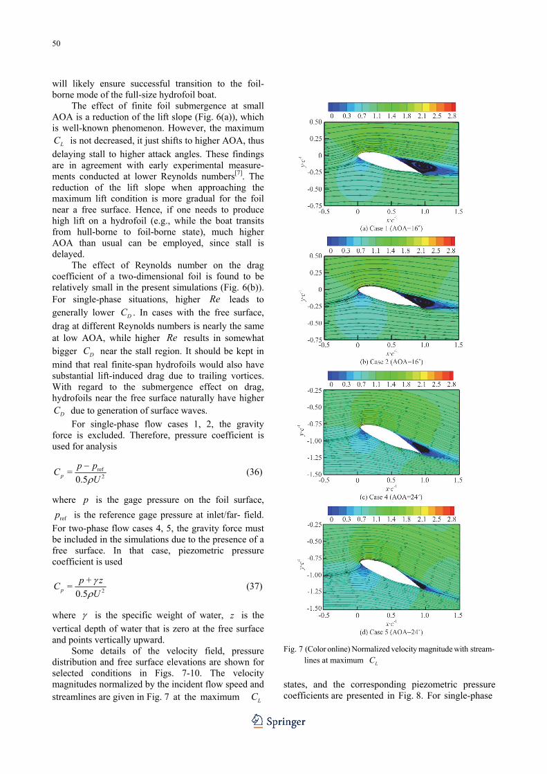
vertical depth of water that is zero at the free surface and points vertically upward. Some details of the velocity field, pressure distribution and free surface elevations are shown for selected conditions in Figs. 7-10. The velocity magnitudes normalized by the incident flow speed and streamlines are given in Fig. 7 at the maximum LC

Fig. 7 (Color online) Normalized velocity magnitude with stream- lines at maximum LC

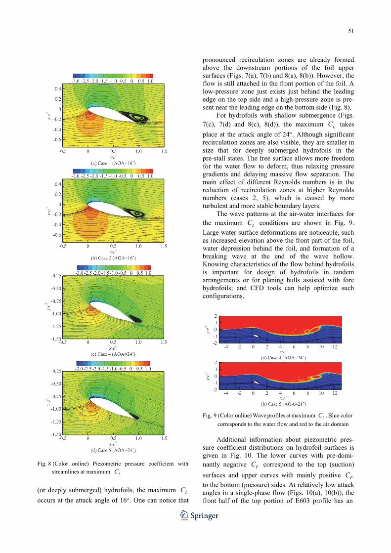
states, and the corresponding piezometric pressure coefficients are presented in Fig. 8. For single-phase

51

Fig. 8 (Color online) Piezometric pressure coefficient with streamlines at maximum LC

(or deeply submerged) hydrofoils, the maximum LC

occurs at the attack angle of 16. One can notice that

pronounced recirculation zones are already formed above the downstream portions of the foil upper surfaces (Figs. 7(a), 7(b) and 8(a), 8(b)). However, the flow is still attached in the front portion of the foil. A low-pressure zone just exists just behind the leading edge on the top side and a high-pressure zone is pre- sent near the leading edge on the bottom side (Fig. 8). For hydrofoils with shallow submergence (Figs. 7(c), 7(d) and 8(c), 8(d)), the maximum LC takes

place at the attack angle of 24. Although significant recirculation zones are also visible, they are smaller in size that for deeply submerged hydrofoils in the pre-stall states. The free surface allows more freedom for the water flow to deform, thus relaxing pressure gradients and delaying massive flow separation. The main effect of different Reynolds numbers is in the reduction of recirculation zones at higher Reynolds numbers (cases 2, 5), which is caused by more turbulent and more stable boundary layers. The wave patterns at the air-water interfaces for the maximum LC conditions are shown in Fig. 9.

Large water surface deformations are noticeable, such as increased elevation above the front part of the foil, water depression behind the foil, and formation of a breaking wave at the end of the wave hollow. Knowing characteristics of the flow behind hydrofoils is important for design of hydrofoils in tandem arrangements or for planing hulls assisted with fore hydrofoils; and CFD tools can help optimize such configurations. Fig. 9 (Color online) Wave profiles at maximum LC . Blue color

corresponds to the water flow and red to the air domain Additional information about piezometric pres- sure coefficient distributions on hydrofoil surfaces is given in Fig. 10. The lower curves with pre-domi- nantly negative PC correspond to the top (suction)

surfaces and upper curves with mainly positive PC

to the bottom (pressure) sides. At relatively low attack angles in a single-phase flow (Figs. 10(a), 10(b)), the front half of the top portion of E603 profile has an

52

Fig. 10 (Color online) Piezometric pressure coefficient extended region with nearly uniform pressure coeffi- cient below -1, producing a dominant contribution to the lift force. At a high attack angle, PC distribution

becomes much less uniform with the greatest suction occurring now near the leading edge, whereas positive

PC on the pressure side increases mainly in the front

portion. Higher Reynolds number leads to slightly larger magnitudes of the pressure coefficient. When the hydrofoil operates near the free water surface, substantial reductions of PC magnitudes

take place at low attack angle of 4 (Figs. 10(c), 10(d)), leading to about 50% drop of the lift coefficient (Fig. 6(a)). At the pre-stall condition with AOA of 24, magnitudes of PC on both pressure and

suction side significantly increase, but mainly in the front portion. The flatter PC zone on the rear part of

the foil top surface is visible at high attack angles (Fig. 10). It can be attributed to the formation of recir- culation bubbles in pre-stall conditions (Figs. 7, 8). 3. Conclusions Two-dimensional, RANS-based computational fluid dynamics simulations have been conducted for a high-lift hydrofoil in a single-phase fluid and in the shallow submergence condition at a moderate Froude number. This modeling approach produced results in good agreement with test data for an airfoil up to the stall regime and for water waves formed behind a hydrofoil. Parametric simulations carried out in a broad range of attack angles showed that the maximum lift coefficient attained at the shallow submergence was about the same as that of the deeply submerged foil. However, the corresponding stall attack angle was about 50% higher in the shallow case than that at the deep submergence for the considered foil profile and flow conditions. This implies that shallow foils can be capable of achieving high lift, albeit at substantially higher (two-dimensional) drag coefficient. Also, the lift produced by hydrofoils at higher Reynolds numbers was found be larger than at smaller Re , especially near the maximum LC

conditions. Hence, model-scale tests with hydrofoil boats likely generate conservative results with regard to the lift capability. Possible future extensions of this research that can be important for practical design of hydrofoil boats include three-dimensional hydrofoils, multi-foil setups, broad range of Froude numbers, and presence of sea waves. Simulations of post-stall regimes and dynamic stall phenomena will likely require more computationally demanding approaches, such as DES or LES-based methods. Acknowledgement This material is based upon research supported by the U. S. Office of Naval Research under Award

53

(Grant No. N00014-17-1-2553). References [1] McLeavy R. Hovercraft and hydrofoils [M]. London, UK:

Janeʼs, 1980. [2] Young Y. L., Harwood C. M., Miguel Montero F. et al.

Ventilation of lifting bodies: Review of the physics and discussion of scaling effects [J]. Applied Mechanics Reviews, 2017, 69(1): 010801.

[3] Rothblum R. S. Investigation of methods of delaying or controlling ventilation on surface piercing struts [D]. Doctoral Thesis, Leeds,UK: University of Leeds, 1977.

[4] Matveev K. I., Wheeler M. P., Xing T. Numerical simu- lation of air ventilation and its suppression on inclined surface-piercing hydrofoils [J]. Ocean Engineering, 2019, 175: 251-261.

[5] Dubrovsky V., Matveev K., Sutulo S. Small waterplane area ships [M]. New York, USA: Backbone publishing, 2007.

[6] Hough G. Froude number effects on two-dimensional hydrofoils [J]. Journal of Ship Research, 1969, 13(1): 53-60.

[7] Nishiyama T. Experimental investigation of the effect of submergence depth upon the hydrofoil section charac- teristics [J]. Journal of Zosen Kiokai, 1959, 1959(105): 7-21.

[8] Ju D. M., Xiang C. L., Wang Z. Y. et al. Flow structures and hydrodynamics of unsteady cavitating flows around hydrofoil at various angles of attack [J]. Journal of Hydrodynamics, 2018, 30(2): 276-286.

[9] Long Y., Long X. P., Ji B. et al. Verification and vali- dation of URANS simulations of the turbulent cavitating flow around the hydrofoil [J]. Journal of Hydrodynamics, 2017, 29(4): 610-620.

[10] Eppler R. Airfoil design and data [M]. Berlin, Germany: Springer Science and Business Media, 2012.

[11] Brizzolara S., Chryssostomidis C. The second generation of unmanned surface vehicles: design features and performance predictions by numerical simulations [C]. Conference ASNE Day, Arlington, VA, USA, 2013.

[12] Brizzolara S., Judge C., Beaver B. High deadrise stepped cambered planing hulls with hydrofoils: SCPH2 [C]. A Proof of Concept. SNAME Chesapeake Power Boat Symposium, Annapolis, MD, USA, 2016.

[13] Wackers J., Guilmineau E., Palmieri A. et al. Hessian- based grid refinement for the simulation of surface- piercing hydrofoils [C]. Proceedings of the 17th Numerical Towing Tank Symposium (NuTTS 2014), Marstrand, Sweden, 2014.

[14] Harwood C. M., Brucker K. A., Miguel F. et al. Expe- rimental and numerical investigation of ventilation inception and washout mechanisms of a surface-piercing hydrofoil [C]. 30th Symposium on Naval Hydrodynamics, Hobart, Australia, 2014.

[15] Duncan J. H. The breaking and non-breaking wave resistance of a two-dimensional hydrofoil [J]. Journal of Fluid Mechanics, 1983, 126: 507-20.

[16] Prasad B., Hino T., Suzuki K. Numerical simulation of free surface flows around shallowly submerged hydrofoil by OpenFOAM [J]. Ocean Engineering, 2015, 102: 87-94.

[17] ANSYS. Fluent User Guide V19.1 [R]. New York, USA: Ansys Inc., 2018.

[18] Menter F. R. Two-equation eddy-viscosity turbulence models for engineering applications [J]. AIAA Journal, 1994, 32(8): 1598-1605.

[19] Xing T., Stern F. Factors of safety for Richardson extrapolation [J]. Journal of Fluids Engineering, 2010, 132(6): 061403.

[20] Xing T., Stern F. Closure to "Discussion of 'Factors of safety for Richardson Extrapolation (2011, ASME J. Fluids Eng., 133, p. 115501)'" [J]. Journal of Fluids Engineering, 2011, 133(11): 115502.

[21] Xing T., Carrica P., Stern F. Computational towing tank procedures for single run curves of resistance and propulsion [J]. Journal of Fluids Engineering, 2008, 130(10): 101102.

[22] Lasauskas E., Naujokaiti L. Analysis of three wing sections [J]. Aviation, 2010, 13(1): 3-10.