Applications of Computational Mechanics in Geotechnical Engineering – Sousa,Fernandes, Vargas Jr & Azevedo (eds)

© 2007 Taylor & Francis Group, London, ISBN 978-0-415-43789-9

Numerical simulations of materials with micro-structure: limit analysisand homogenization techniques

P.B. LourençoUniversity of Minho, Department of Civil Engineering, Guimarães, Portugal

ABSTRACT: Continuum-based numerical methods have played a leading role in the numericalsolution of problems in soil and rock mechanics. However, for stratified soils and fractured rocks,a continuum assumption often leads to difficult parameters to define and over-simplified geometryto be realistic. In such cases, approaches that consider the micro-structure of the material can beadopted. In this paper, two of such approaches are detailed, namely limit analysis incorporatingfractures and individual blocks, and elastoplastic homogenization of layered soils.

1 INTRODUCTION

The present paper addresses the inelastic behavior of heterogeneous media, such as soils and rocks.This problem can be, basically, approached from two directions. A possible direction is to gather,collate and interpret extensive experimental data and, ultimately, manipulate it in the form of mastercurves in terms of non-dimension variables. One step further can be to seek empirical analyticalexpressions that fit the experimental data. However, this approach will not be followed here.Even tough such an approach can be useful, the results are limited to the conditions under whichthe data were obtained. New materials and/or application of a well known material in differentloading conditions lead to a new set of costly experimental programs. Here, a more fundamentalapproach, with a predictive nature, is sought using two different tools, namely limit analysis andhomogenization techniques.

2 LIMIT ANALYSIS

A continuum assumption can lead to difficult parameters to define and over-simplified geometry tobe realistic, particularly in the case of fractured rocks. At least in such case, discrete representationsof fractures and individual blocks must be adopted. Different approaches are possible to representthese heterogeneous media, namely, the discrete element method (DEM), the discontinuous finiteelement method (FEM) and limit analysis (LAn).

The explicit formulation of a discrete (or distinct) element method is detailed in the introductorypaper by Cundall and Strack (1985). The discontinuous deformation analysis (DDA), an implicitDEM formulation, was originated from a back-analysis algorithm to determine a best fit to adeformed configuration of a block system from measured displacements and deformations, Shiand Goodman (1985). The relative advantages and shortcomings of DDA are compared with theexplicit discrete element method and the finite element method (Hart, 1991), even if significantdevelopments occurred in the last decade, particularly with respect to three-dimensional extension,solution techniques, contact representation and detection algorithms. The typical characteristics ofdiscrete element methods are: (a) the consideration of rigid or deformable blocks (in combinationwith FEM); (b) connection between vertices and sides/faces; (c) interpenetration is usually possible;(d) integration of the equations of motion for the blocks (explicit solution) using the real damping

33

coefficient (dynamic solution) or artificially large (static solution). The main advantages are anadequate formulation for large displacements, including contact update, and an independent meshfor each block, in case of deformable blocks. The main disadvantages are the need of a largenumber of contact points required for accurate representation of interface stresses and a rather timeconsuming analysis, especially for 3D problems.

The finite element method remains the most used tool for numerical analysis in solid mechanicsand an extension from standard continuum finite elements to represent jointed rock was developedin the early days of non-linear mechanics, Goodman et al. (1967). On the contrary, limit analysisreceived far less attention from the technical and scientific community for jointed rock, whilebeing very popular for soil problems, Fredlund and Krahn (1977). Still, limit analysis (kinematicapproach) has the advantage of being a simple tool, while having the disadvantages that onlycollapse load and collapse mechanism can be obtained and loading history can hardly be included.Here, a novel implementation of limit analysis is detailed and applied to an illustrative example.

2.1 General formulation

The limit analysis formulation for a rigid block assemblage detailed next adopts the followingbasic hypotheses: the joint between two blocks can withstand limited compressive stresses and theCoulomb’s law controls shear failure, which features non-associated flow given by a zero dilatancyangle.

The static variables, or generalized stresses, at a joint k are selected to be the shear force, Vk , thenormal force, Nk , and the moment, Mk , all at the center of the joint. Correspondingly, the kinematicvariables, or generalized strains, are the relative tangential, normal and angular displacement rates,δnk , δsk and δθk at the joint center, respectively. The degrees of freedom are the displacement ratesin the x and y directions, and the angular change rate of the centroid of each block: δui, δvi and δωi

for the block i. In the same way, the external loads are described by the forces in x and y directions,as well as the moment at the centroid of the block. The loads are split in a constant part (with asubscript c) and a variable part (with a subscript v): fcxi, fvxi, for the forces in the x direction, fcyi,fvyi, for the forces in the y direction, and mci, mvi, for the moments. These variables are collectedin the vectors of generalized stresses Q, generalized strains δq, displacements rates δu, constant(dead) loads Fc, and variable (live) loads Fv. Finally, the load factor α is defined, measuring theamount of the variable load vector applied. The load factor is the limit (minimum) value that theanalyst wants to determine and is associated with collapse.

With the above notation, the total load vector F is given by

2.2 Yield function

The yield function at each joint is composed by the crushing-hinging criterion and the Coulombcriterion. For the crushing-hinging criterion, it is assumed that the normal force is equilibrated bya constant stress distribution near the edge of the joint, see Figure 1a. Here, a is half of the lengthof a joint and w is the width of the joint normal to the plane of the block. The stress value is fcef ,given by Eq. (2), borrowed from concrete limit analysis (Nielsen, 1998). Here, fc is the compressivestrength of the material, and ν is an effectiveness factor, which takes into account reductions inthe compressive strength due to the fact that limit analysis assumes a rigid-plastic behavior, while,in fact, softening occurs. Eq. (3) is an expression for the effectiveness factor commonly used forconcrete (Nielsen, 1998), where fc is expressed in N/mm2.

34

V

ceff

ceff wa

N

M

V

(a) (b)

δθ

δn

-N-M

−N

Figure 1. Joint failure: (a) generalized stresses and strains for the crushing-hinging failure mode;(b) geometric representation of a half of the yield surface.

The constant stress distribution hypothesis leads to the yield function ϕ given by Eq. (4), relatedto the equilibrium of moments; note that Nk represents a non-positive value. The Coulomb crite-rion is expressed by Eq. (5), related to the equilibrium of tangential forces. Here, µ is the frictioncoefficient or the tangent of friction angle at the joint. The equilibrium of normal forces is auto-matically ensured by the rectangular distribution of normal stresses. It is noted that the completeyield function is composed by four surfaces, two surfaces given by Eq. (4) and two surfaces givenby Eq. (5), in view of the use of the absolute value operator. Figure 1b represents half of the yieldsurface (M< 0), while the other half (M > 0) is symmetric to the part shown.

2.3 Flow rule

Figure 1a illustrates also the flow mode corresponding to crushing-hinging, in agreement withthe normality rule. It is noted that, for the Coulomb criterion, the flow consists of a tangentialdisplacement only. The flow rule at a joint can be written, in matrix form, as given by Eq. (6), and,in a component-wise form, as given by Eq. (7), in which the joint subscripts have been dropped forclarity. Here, N0k is the flow rule matrix at joint k and δλk is the vector of the flow multipliers, witheach flow multiplier corresponding to a yield surface, and satisfying Eqs. (8-9). These equationsindicate that plastic flow must involve dissipation of energy, Eq. (8), and that plastic flow cannotoccur unless the stresses have reached the yield surface, Eq. (9). For the entire model, the flow ruleresults in Eq. (10), where the flow matrix N0 can be obtained by assembling all joints matrices.

35

γk

βj

βi

d

dj

i

block i

block j

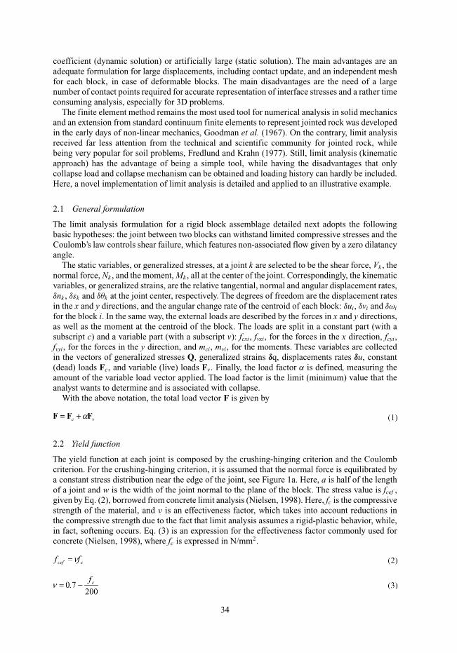
Figure 2. Representation of main geometric parameters.

2.4 Compatibility

Compatibility between joint k generalized strains, and the displacement rates of the adjacent blocksi and j, is given in Eq. (11), being the vector δui defined in Eq. (12) and the compatibility matrixCk ,i, given in Eq. (13). Similarly, the vector δuj and the matrix Ck ,j can be obtained. In this lastequation γk , βi, βj , are the angles between the x axis and, the direction of joint k , the line definedfrom the centroid of block i to the center of joint k , and the line defined from the centroid of blockj to the center of joint k , respectively. Variables di, dj , represent the distances from the center ofjoint k to the centroid of the blocks i and j, respectively, see Figure 2.

Compatibility for all the joints in the model is given by Eq. (14), in which the compatibilitymatrix C is obtained by assembling the corresponding matrices for the joints of the model.

2.5 Equilibrium

Applying the contragredience principle, the equilibrium requirement is expressed by Eq. (15).

2.6 The mathematical programming problem

The solution to a limit analysis problem must fulfill the previously discussed principles. In the pres-ence of non-associated flow, there is no unique solution satisfying these principles and the actualfailure load corresponds to the mechanism with a minimum load factor (Baggio and Trovalusci,1998). The proposed mathematical description results in the non-linear programming (NLP) prob-lem expressed in Eqs. (16–22). Here, Eq. (16) is the objective function and Eq. (17) guarantees bothcompatibility and flow rule. Eq. (18) is a scaling condition of the displacement rates that ensuresthe existence of non-zero values. This expression can be freely replaced by similar equations, as,

36

at collapse, the displacement rates are undefined and it is only possible to determine their relativevalues. Equilibrium is given by Eq. (19), and Eq. (20) is the expression of the yield condition,which together with the flow rule, Eq. (21), must fulfill Eq. (22).

Subject to:

This set of equations represents a case known in the mathematical programming literature asa Mathematical Problem with Equilibrium Constraints (MPEQ) (Ferris and Tin-Loi, 2001). Thistype of problems is hard to solve because of the complementarity constraint, Eq. (22). The solutionstrategy adopted here is that proposed by Ferris and Tin-Loi (2001). It consists of two phases, in thefirst, a Mixed Complementarity Problem (MCP), constituted by Eqs. (17–22) is solved. This givesa feasible initial solution. In the second phase, the objective function, Eq. (16), is reintroducedand Eq. (22) is substituted by Eq. (23). This equation provides a relaxation in the complementarityconstraint, turns the NLP easier to solve, and allows to search for smaller values of the load factor.The relaxed NLP problem is solved for successively smaller values of ρ to force the complementarityterm to approach zero.

It must be said that trying to solve a MPEQ as a NLP problem does not guarantee that the solutionis a local minimum (Ferris and Tin-Loi, 2001). Nevertheless, this procedure seems computationallyefficient and provides solutions of better quality than other strategies tried previously, see Orduñaand Lourenço (2001).

2.7 Computer implementation

The main objective of this work is to develop an analysis tool suitable to be used in practicalengineering projects. For this reason, the computer implementation is done resorting to AutoCAD,in which the geometry of the blocky medium is drawn. The application, developed with VisualBasic for Applications within AutoCAD (ActiveX and VBA 1999), extracts the geometric dataand pre-processes it. Complementary data is added such as volumetric weight, block thickness(typically 1 m for 2D geotechnical problems), friction coefficient and compressive strength. Thelimit analysis is done within the modeling environment GAMS (GAMS, 1998), which allows theuser to develop large and complex mathematical programming models, and solve them with state ofthe art routines. The previously mentioned CAD package is used as post-processor to draw failuremechanisms.

2.8 Application

Validation of the formulation and the implementation of the 2D model is given in Orduña andLourenço (2003), while the extension to 3D is fully detailed in Orduña and Lourenço (2005a,b).Here, to demonstrate the applicability of limit analysis to geotechnical problems, an example of

37

Figure 3. Evolution of a possible collapse mechanism in a tunnel excavated in a jointed rock mass.

shallow depth tunnel in fractured rock under increasing surface loads is simulated in Figure 3,see Jing (1998) for additional details. The problem geometry is formed by a rectangular domaincontaining two sets of random fractures.A rectangular tunnel is assumed to be excavated at the centreof the area. A vertical downward load due to self-weight appears and the other three boundariesare fixed in their respective normal directions. This problem has no practical implications and justserves as a demonstration.

3 HOMOGENIZATION TECHNIQUES

The chief disadvantage of the methods addressed in the previous section is the requirement forknowing the exact geometry of fracture systems in the problem domain. This condition can rarelybe met in practice. This difficulty, however, exists for all mathematical models including thosebased on a continuum approach. The difference is how different approaches deal with this intrinsicdifficulty. The continuum approach chooses to trade the geometrical simplicity over the materialcomplexity by introducing complex constitutive laws and properties for an equivalent continuumthrough a proper homogenization process, which is only valid on the foundation of a “representativeelementary volume”(REV). If this REV cannot be found or becomes too large (larger than the sizeof the excavation concerned, for example) then the continuum approach cannot be justified. But,in several cases, the continuum approach can be of relevance. Here, the problem of layered naturalor reinforced soils is addressed by means of homogenization techniques.

3.1 General considerations

Composite materials consist of two or more different materials that form regions large enough tobe regarded as continua and which are usually bonded together by an interface. Two kinds of infor-mation are needed to determine the properties of a composite material: the internal constituents’geometry and the physical properties of the phases. Many natural and artificial materials are imme-diately recognized to be of this nature, such as: laminated composites (as used in the aerospace andtire industry), alloys, porous media, cracked media (as jointed rocked masses), masonry, laminatedwood, etc. However a lot of composite materials are normally assumed homogeneous. For example,this is the case of concrete, even if at a meso-level aggregates and matrix are already recognizable,and metals, in fact polycrystalline aggregates.

38

Figure 4. Representative volume element in a composite body.

The existence of randomly distributed constituents was one of the first problems to be discussedby researchers, see Paul (1960), Hashin and Shtrikman (1962) and Hill (1963). The Hashin-Shtrikman bounds were derived from a variational principle and knew some popularity but they areonly valid for arbitrary statistically isotropic phase geometry, see Figure 4. An additional conditionfor the practical use of these bounds is that the constituents stiffness ratios are small, see Hashin andShtrikman (1962) and Watt and O’Connell (1980). They cannot obviously provide good estimatesfor extreme constituent stiffness ratios such as one rigid phase or an empty phase (porous or crackedmedia). This precludes the use of the above results for inelastic behavior where extremely largestiffness ratios will be found.

The basis underlying the above approach is however important. It is only natural that techniquesto regard any composite as an homogeneous material are investigated, provided that the model sizeis substantially larger than the size of the inhomogenities. In fact all phenomena in a compositematerial are described by differential equations with rapidly oscillating coefficients. This rendersnumerical solutions practically impossible since too small meshes must be considered.

Consequently, effective constitutive relations of composite structures are of great importance inthe global analysis of this type of media by numerical techniques (e.g. the Finite Elements Method).For this reason the rather complicated structure of a particular composite type is replaced by aneffective medium by using a technique known as homogenization method or effective mediumtheory. Several mathematical techniques of different complexity are available to solve the prob-lem, Sanchez-Palencia (1980, 1987), Suquet (1982) but for periodic structures the method of“Asymptotic Analysis” has renown some popularity, see also Bakhvalov and Panasenko (1989)and Bensoussan et al. (1978). The extension of these methods to inelastic behavior is however notsimple. Knowledge of the actual macro- or homogenized constitutive law requires knowledge ofan infinite number of internal variables, namely the whole set of inelastic micro-strains. Howeversome simplified models with piecewise constants inelastic strains can be proposed (as carried outin this paper).

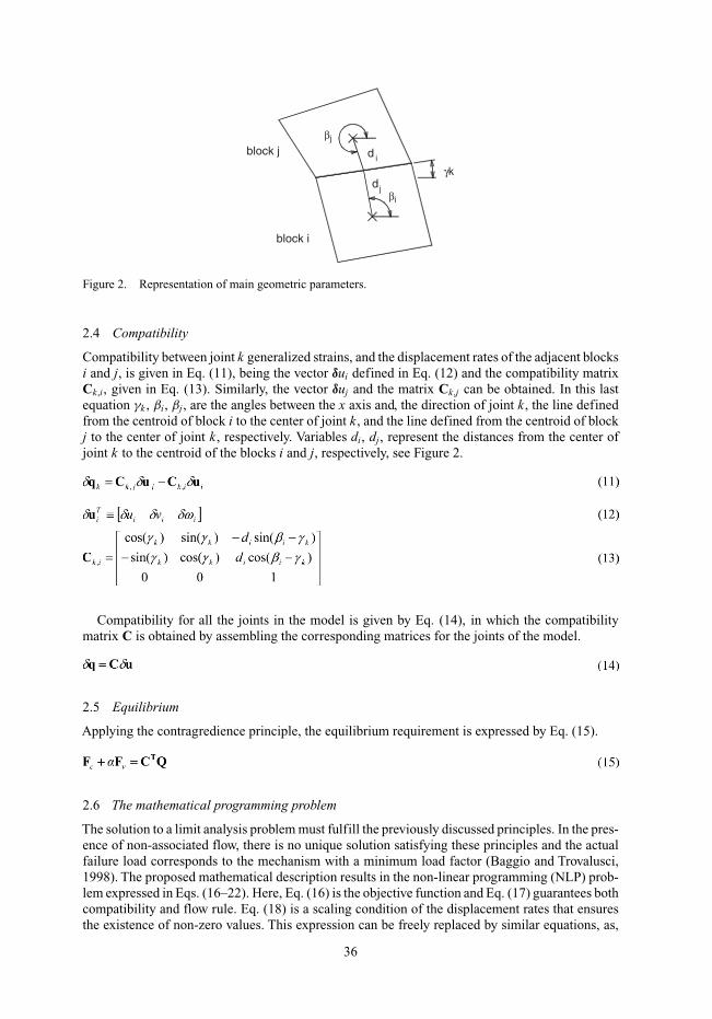
The objective of the homogenization process is to describe the composite material behavior fromthe behavior of the different components. This problem has known a large importance in the lastdecade due to the increasing use and manufacture of composites. To solve the present problemsome simplifications are necessary and attention is given only to the special case of laminatedor layered composites. This means that the geometry of the phases are known, which simplifiesenormously the task of finding equivalent elastic properties for the medium. The composite materialexamined is made of laminae stacked at various orientations, the only restriction being imposedon the periodicity of the lamination along the structures (see Figure 5), which is usually fulfilledin numerous engineering applications. Examples include aerospace industries, laminated wood,stratified or sedimentary soils, stratified rock masses, etc.

39

Figure 5. The periodic laminated composite material and the structure of the unit cell.

Figure 6. Unit cell. Representative prism for system of parallel orthotropic layers.

3.2 Theory

In the previous section a reference is made to the mathematical techniques of homogenizationof periodic structures. The asymptotic expansion of the displacement and stress fields is usedfor example in Paipetis et al. (1993) to obtain the elastic stiffness of a homogenized continuum.The solution is however presented in an explicit form for each coefficient of the stiffness matrix.This solution is not practical for computational implementation and almost precludes the use ofhomogenization techniques for inelastic behavior.

Here, the approach originated in the field of rock mechanics will be discussed, see Salamon(1968) and Gerrard (1982), and recast in matrix form. For that purpose the layered material shownin Figure 5 is considered again, built from a repeating system of parallel layers, each of whichconsists of orthotropic elastic material. This means that the material properties of each layer havethree mutually perpendicular planes of symmetry. The layers are aligned so that each set of threeplanes are respectively perpendicular to a single set of Cartesian coordinates (x1, x2 and x3). Thenotation selected for the axes is intentionally different than the usual (x, y, z axes) to draw theattention to the fact that the x1, x2 and x3 axes are placed on the material symmetry axes. The unitcell, in the form of a representative prism, is shown in Figure 6. The homogenization direction (x3)is normal to the layering planes and, hence, for each layer, one of the planes of elastic symmetryis parallel to the layering planes. In this direction the dimension of the prism is defined by theperiodicity of the structure and in the other two directions a unit length can be assumed.

It is assumed that the system of layers remains continuous after deformation and that no relativedisplacement takes place in the interfaces between layers. The latter assumption simplifies theproblem to great extent but, at least mathematically, discontinuities in the displacements field canbe incorporated, see Bakhalov and Panasenko (1989). The prism representative of the compositematerial is further assumed to be subjected to homogeneous distributions of stress and strain,meaning that the volume of the prism must be sufficiently small to make negligible, in the equivalent

40

medium, the variation of stresses and strains across it. The objective is to obtain a macro- orhomogenized constitutive relation between homogenized stresses σ and homogenized strains ε,

where Dh is the homogenized stiffness matrix.

3.3 Elastic formulation

The macro-constitutive relation is obtained from the micro-constitutive relations. For the ith layerthe relation between the (micro-)stress σ i and the (micro-)strains εi is given by the (micro)stiffnessmatrix Di and reads

In order to establish the relationships between stresses and strains in a homogenized continuum,the following averaged quantities in an equivalent prism are defined:

where V is the volume of the representative prism and j indicates all the components of the stressand strain tensors.

Auxiliary stresses (t1, t2 and t12) and auxiliary strains (e3, e13 and e23) are introduced as a deviationmeasure of the ith layer stress/strain state from the averaged values. Under the assumptions givenabove, the stress components for the ith layer read

and the strain components for the ith layer read

Now let the thickness of the ith layer be hi and the normalized thickness pi be defined as

where L is the length of the representative prism in the x3 direction. Substitution of Eqs. (27) inEqs. (26.1) yields the following conditions for the auxiliary stress components:

Similarly, from Eqs. (28) and Eqs. (26.2), the auxiliary strain components are constraint by

Note that, if the conditions given in the above equations are fulfilled, then the strain energystored in the representative prism and the equivalent prism are the same.

A vector of auxiliary stresses is now defined as t i, given by

41

and the vector of auxiliary strains ei is defined as

It is noted that half of the components of the auxiliary stress and strain vectors are zero, see Eqs.(27,28). If the non-zero components are assembled in a vector of unknowns, xi, defined as

where the projection matrix into the stress space, P t , and the projection matrix into the strain space,Pe, read

for homogenization along the axis x1,

for homogenization along the axis x2 and

for homogenization along the axis x3.Now, the auxiliary stresses can be redefined as

and the auxiliary strains as

The stresses and strains in the ith layer read

Incorporating these equations in Eq. (25) leads to

By using Eqs. (38, 39), further manipulation yields

which can be recast as

This equation yields, finally, the relation between averaged stresses and strains, as

42

Here, the homogenized linear elastic stiffness matrix, Dh, reads

Once the averaged stresses and strains are known, also the stresses and strains in the ith layer canbe calculated. Using Eq. (42), the vector of unknowns xi can be calculated. Algebraic manipulationyields

and

Here, the transformation matrices T ti and T ei read

where I is the identity matrix.

3.4 Elastoplastic formulation

For plasticity the form of the elastic domain is defined by a yield function f < 0. Loading/ unloadingcan be conveniently established in standard Kuhn-Tucker form by means of the conditions

where.

λ is the plastic multiplier rate. Here it will be assumed that the yield function is of the form

where κ is introduced as a measure for the amount of hardening or softening and �, σ representgeneric functions. The usual elastoplastic relation hold: the total strain increment �ε is decomposedinto an elastic, reversible part �εeand a plastic, irreversible part �εp

the elastic strain increment is related to the stress increment by the elastic constitutive matrix D as

and the assumption of associated plasticity yields

The scalar κ introduced before reads, in case of strain hardening,

where the diagonal matrix Q = diag{ 1, 1, 1, ½, ½, ½, ½}, and, in case of work hardening,

43

The integration of the constitutive equations above is a problem of evolution that can be regardedas follows. At a stage n the total strain and plastic strain fields as well as the hardening parameter(s)(or equivalent plastic strain) are known:

Note that the elastic strain and stress fields are regarded as dependent variables that can be alwaysbe obtained from the basic variables through the relations

Therefore, the stress field at a stage n + 1 is computed once the strain field is known. The problemis strain driven in the sense that the total strain ε is trivially updated according to the exact formula

It remains to update the plastic strains and the hardening parameter(s). These quantities are deter-mined by integration of the flow rule and hardening law over the step n → n + 1. In the frame of afully implicit Euler backward integration algorithm this problem is transformed into a constrainedoptimization problem governed by discrete Kuhn-Tucker conditions as shown by Simo et al (1988).

It has been shown in different studies, e.g. Ortiz and Popov (1985) and Simo and Taylor (1986),that the implicit Euler backward algorithm is unconditionally stable and accurate for J2-plasticity.

This algorithm results in the following discrete set of equations:

in which �κn+1 results from Eq. (54) or Eq. (55) and the elastic predictor step returns the value ofthe elastic trial stress σ trial

Application of the above algorithm to the homogenized material equivalent to the layered materialshown in Figure 6 results in increasing difficulties. The homogenized material consists of severallayers with individual elastic and inelastic properties. As given in Eqs. (46–47), different stressesand strains are obtained for each layer, which are again different from the average stresses andstrains.

Due to this feature and the fact that inelastic behavior is considered for the layers, for a given strainincrement in the equivalent material it is not possible to calculate immediately the correspondentstrain increments for each layer. This precludes the use of a standard plasticity algorithm due to thefact that the algorithm is strain driven. An equivalent return mapping must be carried out, in whichall the layers are considered simultaneously. The equivalent return mapping is, therefore, a returnmapping in all the layers (or a return mapping in terms of average strains and average stresses).This has some similitude with the fraction model, Besseling (1958).

Here only the simple case of J2-plasticity is addressed, being the reader addressed to Lourenço(1995) for other cases. The Von Mises yield criterion can be written in a matrix form and reads

44

where the projection matrix P reads

For this yield surface, holds the well-known relation

both for a strain or work hardening rule. From the standard algorithm shown above, cf. eq. (59), itis straightforward to obtain the update of the stress vector σn+1 as

where the mapping matrix A reads

Note that the mapping matrix is only a function of �λn+1, i.e. A =A(�λn+1). If the individuallayers are considered, Eq. (64) for the ith layer must be rewritten as

where the mapping matrix, Ai, is a function of �λn+1,i and the elastic trial stress σ triali , cf. Eq. (60),

reads

If all the layers are now considered simultaneously, the question arises whether one particularlayer is elastic or plastic, but this will be considered trivial in the present note. In fact, in case of anelastic layer, Eq. (67) remains valid if the mapping matrix is redefined as the identity matrix (i.e.�λn+1 = 0),

Inserting Eq. (40) in Eq. (66), the latter can be rewritten in terms of average stresses and strains(σ and ε) and auxiliary stresses and strains of the ith layer (t i and ei) at stage n + 1 as

If a modified trial stress for the ith layer is defined as

(note that the average strain is included in the expression instead of the strain of the ith layer), Eq.(69) reads

45

Inserting Eqs. (38,39) in this equation and further manipulation, see Lourenço (1996), leads tothe update of the average stress as

Note that the summation above is extended to all the layers (elastic and plastic). The returnmapping procedure is now established in a standard way. From the average stresses it is possible tocalculate the stresses in the ith layer. At this point it is clear that a system of non-linear equations in�λn+1

′s can be built: fi(�λn+1,1, . . . , �λn+1, j) = 0, i = 1, . . . , j. This system of non-linear equationscan be solved by any mathematical standard technique and has so many unknowns (and equations)as the number of plastic layers. Finally, when convergence is reached the state variables (ε, εp

and κ) can be updated. For a discussion of the algorithm implementation and the calculation of theconsistent tangent operator the reader is referred to Lourenço (1996).

3.5 Extension to a Cosserat continuum

Physical arguments in favor of a Cosserat approach in granular materials have been put forward inMühlhaus and Vardoulakis (1987). However, the very important feature of a Cosserat continuumis the introduction of a characteristic length in the constitutive description, thus rendering thegoverning set of equations elliptic while allowing for localization of deformation in a narrow, butfinite band of material. The excessive dependence of standard continua upon spatial discretizationcan be then obviated or, at least, considerably reduced.

The implementation carried out is based on the original work of de Borst (1991, 1993) on thetwo-dimensional elastoplastic Cosserat continuum and the extension of Groen et al. (1994) to thethree-dimensional case, see Lourenço (1996) for details.

3.6 Validation

In the following examples the described algorithm is tested by considering a material built from twolayers, viz. a “weak” and a “strong” layer. Different elastic and inelastic behavior is assumed forboth layers. Large scale calculations are carried out in (average) plane strain and three-dimensionalapplications. The objective is to assess the performance of the theory in a different class of problemsranging from highly localized to distributed failure modes. For this purpose, different calculationsof the same model with increasing number of layers are carried out (note that layer in this sectionwill be generally assumed as the repeating pattern, i.e. one layer contains two different materials, aweak and a strong layer). Convergence to the homogenized solution must be found upon increasingthe number of layers.

The same fictitious material, described in Lourenço (1996), is used throughout this section. Inthe large calculations, 2D quadratic elements (8-noded quads) with 2 × 2 Gauss integration areused and 3D quadratic elements (20-noded bricks) with 3 × 3 Gauss integration are used. For theelastoplastic calculations a (local) full Newton-Raphson method is used in the return mappingalgorithm with a 10−7 tolerance for all equations and a (global) full Newton-Raphson method isused to obtain convergence at global level. The tolerance is set to an energy norm of 10−4.

The first example is a rigid foundation indented into a stratified soil (see Figure 7). Only half ofthe mesh is considered due to symmetry conditions. This example is meant to assess the performanceof the homogenization technique under plane strain conditions in situations not only constrainedby the material behavior, but also by geometric constraints. Clearly a localized failure is obtainedaround the indentation area.

A comparison is given between the 2D (plane strain) homogenized continuum and three different2D (plane strain) layered discretizations: 8, 16 and 32 equivalent material layers (see Figure 8).Note that the zero normal strain condition introduces a three dimensional state of stress, meaningthat all the calculations can be carried out under plane strain conditions. The results obtained in a

46

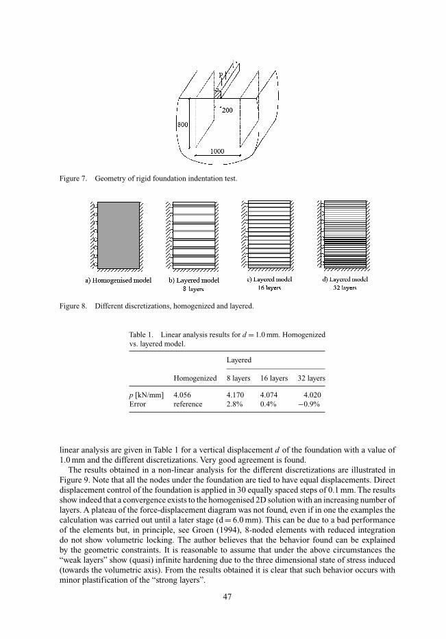
Figure 7. Geometry of rigid foundation indentation test.

Figure 8. Different discretizations, homogenized and layered.

Table 1. Linear analysis results for d = 1.0 mm. Homogenizedvs. layered model.

Layered

Homogenized 8 layers 16 layers 32 layers

p [kN/mm] 4.056 4.170 4.074 4.020Error reference 2.8% 0.4% −0.9%

linear analysis are given in Table 1 for a vertical displacement d of the foundation with a value of1.0 mm and the different discretizations. Very good agreement is found.

The results obtained in a non-linear analysis for the different discretizations are illustrated inFigure 9. Note that all the nodes under the foundation are tied to have equal displacements. Directdisplacement control of the foundation is applied in 30 equally spaced steps of 0.1 mm. The resultsshow indeed that a convergence exists to the homogenised 2D solution with an increasing number oflayers. A plateau of the force-displacement diagram was not found, even if in one the examples thecalculation was carried out until a later stage (d = 6.0 mm). This can be due to a bad performanceof the elements but, in principle, see Groen (1994), 8-noded elements with reduced integrationdo not show volumetric locking. The author believes that the behavior found can be explainedby the geometric constraints. It is reasonable to assume that under the above circumstances the“weak layers” show (quasi) infinite hardening due to the three dimensional state of stress induced(towards the volumetric axis). From the results obtained it is clear that such behavior occurs withminor plastification of the “strong layers”.

47

Figure 9. Force-displacement diagrams for different discretisations.

Figure 10. Deformed mesh for different discretizations (×15).

Figure 11. Equivalent plastic strain for different discretizations (>0.5 × 10−4).

Fig. 10 shows the deformed meshes and Fig. 11 illustrates the plastic points at failure for thedifferent discretizations. The deformation patterns of the layered models show some bending ofthe strong layers. This cannot be reproduced in the homogenized model.

It is important to point out that the foundation was assumed to be located in the middle planeof the strongest material. For examples with a small number of layers, due to the extremely largestress gradients around the geometrical discontinuities, some differences can be expected.

The collapse of a 45◦ slope subjected to its own weight (g) is now considered (see Figure 12).Again different discretizations are considered: the plane strain homogenized model and the planestrain layered model (4, 8 and 16 layers). The results of the maximum vertical displacement in

48

Figure 12. Different discretizations, homogenized and layered.

Table 2. Linear analysis results for g = 1.0 N/mm3. Homogenizedvs. layered model

Layered

Homogenized 4 layers 8 layers 16 layers

Disp. y [mm] −25.47 −27.88 −26.70 −26.09Error reference 9.5% 4.8% 2.4%

Figure 13. Force-displacement diagrams for different discretizations.

the slope obtained in a linear analysis are given in Table 2 for a weight value g with a value of1.0 N/mm3 and the different discretisations. Good agreement is found.

The results obtained in a non-linear analysis for the different discretizations are illustrated inFigure 13. Indirect displacement control of the top left corner is applied in 30 equally steps of0.2 mm. In this case even for a small number of layers the difference is minimal (1.8%). Figure 14shows the deformed meshes and it is remarkable that such a close agreement is found in respectto the shear band formation. Figure 15 illustrates the plastic points at failure for the homogenizedmodel in the two different materials (these results agree well with the layered model). The plasticpoints of the different materials are not shown in a single picture because different scales are used.The inelastic behavior of the weak material close to the bottom support is substantially larger thanthe diagonal shear failure.

It is important to point out that the bottom layer was assumed to be from the weak material. Thishas some influence on the results, especially if only a few layers are considered. This assumptionis also the reason for the force-displacement diagram of the layered models being less stiff thanthe homogenized result (remember that the slope is subjected to self weight loading). If the bottomlayer was assumed to be from the strong material, the force-displacement diagram of the layeredmodels would be stiffer than the homogenized result.

Finally, a last example is considered in order to assess the formulation of the homogenizationcontinuum for truly three-dimensional finite elements. For this purpose, the collapse of an embank-ment subjected to its own weight (g) is analyzed. Again different discretizations are considered:the 3D homogenized model and the 3D layered model with 4 and 8 equivalent material layers

49

Figure 14. Deformed mesh for different discretizations (×15).

Figure 15. Equivalent plastic strain for different discretizations (>0.5 × 10−4).

Figure 16. Different discretizations, homogenized and layered.

Table 3. Linear analysis results for g = 1.0 N/mm3 (displacementof the free corner). Homogenized vs. layered model

Layered

Homogenized 4 layers 8 layers

Disp. z [mm] −29.06 −30.29 −29.63Error reference 4.2% 2.0%

(see Figure 16). The results obtained in a linear analysis are given in Table 3 for a weight g with avalue of 1.0 N/mm3 and the different discretizations. Good agreement is found.

The results obtained in a non-linear analysis for the different discretizations are illustrated inFigure 17. Indirect displacement control of the free corner is applied in 20 equally spaced steps of0.3 mm. The results show indeed that a convergence exists to the 3D homogenised solution with

50

Figure 17. Force-displacement diagrams for different discretizations.

Figure 18. Total deformed mesh for different discretizations (×10).

Figure 19. Incremental deformed mesh for different discretizations (×300).

an increasing number of layers. In this case even for a small number of layers the difference isminimal (1.5%). Figures 18 and 19 show the deformed meshes at failure (total and incremental) forthe different discretizations. Note that, even for the incremental displacements, a good agreement isfound between the 3D homogenised model and the 3D layered model (8 layers). As in the previousexample, it is important to point out that the bottom layer was assumed to be from the weak material.

4 CONCLUSIONS

The difficulties involved the numerical modeling of non-homogeneous continuum media are wellknown. Different approaches are possible to represent heterogeneous media, namely, the discreteelement method, the finite element method and limit analysis. Here, two approaches have beendetailed.

The first approach considered is limit analysis of fracture or slip lines, together with individualrigid blocks. The adopted formulation assumes, besides the standard Coulomb friction law, a

51

compression limiter and non-associated flow. This results in a non-linear optimization problemthat can be successfully solved with state of the art techniques. An example of application to theexcavation of a tunnel in fractured rock is shown.

The second approach considered is the elastoplastic homogenization of layered media. A matrixformulation is proposed with straightforward extension to inelastic problems. Several examples ofvalidation and application to stratified or reinforced soils are shown.

REFERENCES

ActiveX and VBA developer’s guide. 1999. Autodesk.Baggio, C. & Trovalusci, P. 1998. Limit analysis for no-tension and frictional three-dimensional discrete

systems. Mechanics of Structures and Machines 26(3): 287–304.Bakhvalov, N. & Panasenko, G. 1989. Homogenisation: averaging processes in periodic media. Dordrecht :

Kluwer Academic Publishers.Bensoussan, A., Lions, J.-L. & Papanicolaou, G. 1978. Asymptotic analysis of periodic structures. Dordrecht :

Kluwer Academic Publishers.Besseling, J.F. 1958. A theory of elastic, plastic and creep deformations of an initially isotropic mate-

rial showing anisotropic strain-hardening, creep recovery and secondary creep. J. Appl. Mech. 22:529–536.

Cundall, P.A. & Strack O.D.L. 1979. Discrete numerical-model for granular assemblies. Geotechnique 29 (1):47–65.

de Borst, R. 1991. Simulation of strain localisation: A reappraisal of the Cosserat continuum, Engng. Comput.8: 317–332.

de Borst, R. 1993. A generalisation of J2-flow theory for polar continua, Comp. Meth. Appl. Mech. Engng.103: 347–362.

Ferris, M.C. & Tin-Loi, F. 2001. Limit analysis of frictional block assemblies as a mathematical program withcomplementarity constraints. International Journal of Mechanical Sciences 43: 209–224.

Fredlund D.G. & Krahn J. 1977. Comparison of slope stability methods of analysis. Canadian GeotechnicalJournal 14 (3): 429–439.

GAMS A user’s guide. 1998. Brooke, A., Kendrick, D., Meeraus, A., Raman, R. & Rosenthal, R.E.http://www.gams.com/docs/gams/GAMSUsersGuide.pdf.

Gerrard, C.M. 1982. Equivalent elastic moduli of a rock mass consisting of orthorhombic layers. Int. J. Rock.Mech. Min. Sci. & Geomech. 19: 9–14.

Goodman, R.E., Taylor, R.L. & Brekke T.L. 1968. A model for mechanics of jointed rock. Journal of the SoilMechanics and Foundations Division 94 (3): 637–659.

Groen, A.E. 1994. Improvement of low order elements using assumed strain concepts. Delft : Delft Universityof Technology.

Groen, A.E., Schellekens, J.C.S. & de Borst, R. 1994. Three-dimensional finite element studies of failure insoil bodies using a Cosserat continuum. In: H.J. Siriwardane & M.M. Zaman (eds), Computer Methods andAdvances in Geomechanics: 581–586. Rotterdam: Balkema.

Hart, R.D. 1991. General report: an introduction to distinct element modelling for rock engineering. In:W. Wittke (eds), Proceedings of the of 7th Congress on ISRM : 1881–1892. Rotterdam: Balkema.

Hashin, Z. & Shtrikman, S. 1962. On some variational principles in anisotropic and nonhomogeneous elasticity.J. Mech. Phys. Solids 10: 335–342.

Hill, R. 1963. Elastic properties of reinforced solids: Some theoretical principles. J. Mech. Phys. Solids 11:357–372.

Jing, L. 1998. Formulation of discontinuous deformation analysis (DDA) – an implicit discrete element modelfor block systems. Engineering Geology 49: 371–381.

Lourenço, P.B. 1995. The elastoplastic implementation of homogenization techniques: With an extension tomasonry structures. Delft : Delft University of Technology.

Lourenço, P.B. 1996.A matrix formulation for the elastoplastic homogenisation of layered materials, Mechanicsof Cohesive-Frictional Materials 1: 273–294.

Mühlhaus, H.-B. & Vardoulakis, I. 1987. The thickness of shear bands in granular materials, Geotechnique37: 271–283.

Nielsen, M.P. 1999. Limit Analysis and Concrete Plasticity. Boca Raton : CRC Press.

52

Orduña, A. & Lourenço, P.B. 2001. Limit analysis as a tool for the simplified assessment of ancient masonrystructures. In P.B. Lourenço & P. Roca (eds) Proc. 3rd Int. Seminar on Historical Constructions: 511–520.Guimarães : Universidade do Minho.

Orduña, A. & Lourenço, P.B. 2003. Cap model for limit analysis and strengthening of masonry structures.J. Struct. Engrg. 129(10), 1367–1375.

Orduña, A. & Lourenço, P.B. 2005a. Three-dimensional limit analysis of rigid blocks assemblages. Part I:Torsion failure on frictional joints and limit analysis formulation. Int. J. Solids and Structures 42(18–19):5140–5160.

Orduña, A. & Lourenço, P.B. 2005b. Three-dimensional limit analysis of rigid blocks assemblages. Part II:Load-path following solution procedure and validation. Int. J. Solids and Structures 42(18-19): 5161–5180.

Ortiz, M. & Popov, E.P. 1985. Accuracy and stability of integration algorithms for elastoplastic constitutiverelations. Int. J. Numer. Methods Engrg. 21: 1561–1576.

Paipetis, S.A., Polyzos, D. & Valavanidis, M. 1993. Constitutive relations of periodic laminated compositeswith anisotropic dissipation. Arch. Appl. Mech. 64: 32–42.

Paul, B. 1960. Prediction of elastic constants of multiphase materials. Trans. of AIME 218: 36–41.Salamon, M.D.G. 1968. Elastic moduli of stratified rock mass. Int. J. Rock. Mech. Min. Sci. 5: 519–527.Sanchez-Palencia, E. 1980. Non-homogeneous media and vibration theory. Berlin: Springer.Sanchez-Palencia, E. 1987. Homogenization techniques for composite media. Berlin: Springer.Shi, G. & Goodman, R.E. 1985. Two dimensional discontinuous deformation analysis. Int. J. NumericalAnalyt.

Meth. Geomech. 9, 541–556.Simo, J.C. & Taylor, R.L. 1986. A return mapping for plane stress elastoplasticity. Int. J. Numer. Methods

Engrg. 22: 649–670.Simo, J.C., Kennedy, J.G. & Govindjee, S. 1988. Non-smooth multisurface plasticity and viscoplasticity.

Loading/unloading conditions and numerical algorithms. Int. J. Numer. Methods Engrg. 26: 2161–2185.Suquet, P. 1982. Plasticité et homogénéisation. PhD Dissertation. Paris : Université de Paris.Watt, J.P. & O’Connell, R.J. 1980. An experimental investigation of the Hashin-Shtrikman bounds on twophase

aggregate elastic properties. Physics of Earth and Planetary Interiors 21: 359–370.

53