NUMERICAL SIMULATIONS OF HEAT TRANSFER AND FLUID …rpacheco/RES/PUB/nht1.pdf · NUMERICAL...

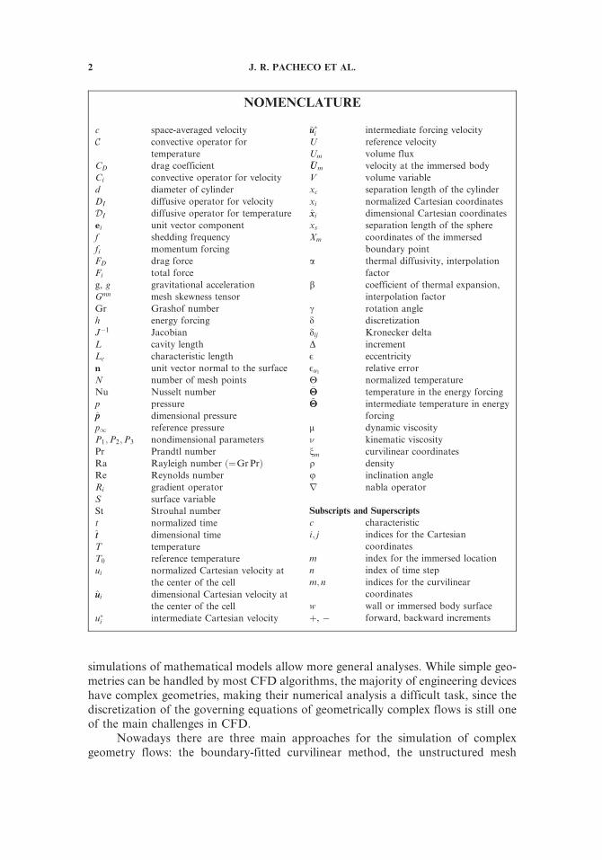
NUMERICAL SIMULATIONS OF HEAT TRANSFERAND FLUID FLOW PROBLEMS USING ANIMMERSED-BOUNDARY FINITE-VOLUME METHODON NONSTAGGERED GRIDS

J. R. PachecoMechanical and Aerospace Engineering Department, Arizona State University,Tempe, Arizona, USA

A. Pacheco-VegaCIEP—Facultad de Ciencias Quımicas, Universidad Aut�oonoma de San LuisPotosı, San Luis Potosı, Mexico

T. RodicMechanical and Aerospace Engineering Department, Arizona State University,Tempe, Arizona, USA

R. E. PeckMechanical and Aerospace Engineering Department, Arizona State University,Tempe, Arizona, USA

This article describes the application of the immersed boundary technique for simulating

fluid flow and heat transfer problems over or inside complex geometries. The methodology

is based on a fractional step method to integrate in time. The governing equations are dis-

cretized and solved on a regular mesh with a finite-volume nonstaggered grid technique.

Implementations of Dirichlet and Neumann types of boundary conditions are developed

and completely validated. Several phenomenologically different fluid flow and heat transfer

problems are simulated using the technique considered in this study. The accuracy of the

method is second-order, and the efficiency is verified by favorable comparison with previous

results from numerical simulations and laboratory experiments.

1. INTRODUCTION

One of the main streams in the analysis and design of engineering equipmenthas been the application of computational fluid dynamics (CFD) methodologies.Despite the fact that experiments are important to study particular cases, numerical

Received 15 July 2004; accepted 30 December 2004.

The authors would like to thank Ms. Renate Mittelmann from the Department of Mathematics at

Arizona State University for access to computer facilities. We also acknowledge the useful comments of

Dr. Andrew Orr from University College London and of the anonymous referees for bringing to our

attention the immersed continuum method.

Address correspondence to J. R. Pacheco, ASU P.O. Box 6106, Tempe, AZ 85287-6106, USA.

E-mail: [email protected]

1

Numerical Heat Transfer, Part B, 48: 1–24, 2005

Copyright # Taylor & Francis Inc.

ISSN: 1040-7790 print=1521-0626 online

DOI: 10.1080/10407790590935975

simulations of mathematical models allow more general analyses. While simple geo-metries can be handled by most CFD algorithms, the majority of engineering deviceshave complex geometries, making their numerical analysis a difficult task, since thediscretization of the governing equations of geometrically complex flows is still oneof the main challenges in CFD.

Nowadays there are three main approaches for the simulation of complexgeometry flows: the boundary-fitted curvilinear method, the unstructured mesh

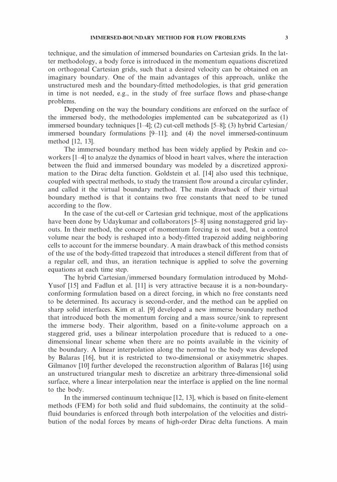
NOMENCLATURE

c space-averaged velocity

C convective operator for

temperature

CD drag coefficient

Ci convective operator for velocity

d diameter of cylinder

DI diffusive operator for velocity

DI diffusive operator for temperature

ei unit vector component

f shedding frequency

fi momentum forcing

FD drag force

Fi total force

g, g gravitational acceleration

Gmn mesh skewness tensor

Gr Grashof number

h energy forcing

J�1 Jacobian

L cavity length

Lc characteristic length

n unit vector normal to the surface

N number of mesh points

Nu Nusselt number

p pressure

pp dimensional pressure

p1 reference pressure

P1;P2;P3 nondimensional parameters

Pr Prandtl number

Ra Rayleigh number ð¼GrPrÞRe Reynolds number

Ri gradient operator

S surface variable

St Strouhal number

t normalized time

tt dimensional time

T temperature

T0 reference temperature

ui normalized Cartesian velocity at

the center of the cell

uui dimensional Cartesian velocity at

the center of the cell

u�i intermediate Cartesian velocity

~uu�i intermediate forcing velocity

U reference velocity

Um volume flux�UUm velocity at the immersed body

V volume variable

xc separation length of the cylinder

xi normalized Cartesian coordinates

xxi dimensional Cartesian coordinates

xs separation length of the sphere

Xm coordinates of the immersed

boundary point

a thermal diffusivity, interpolation

factor

b coefficient of thermal expansion,

interpolation factor

c rotation angle

d discretization

dij Kronecker delta

D increment

E eccentricity

Eu1 relative error

H normalized temperature�HH temperature in the energy forcing~HH intermediate temperature in energy

forcing

m dynamic viscosity

n kinematic viscosity

nm curvilinear coordinates

q density

u inclination angle

r nabla operator

Subscripts and Superscripts

c characteristic

i; j indices for the Cartesian

coordinates

m index for the immersed location

n index of time step

m; n indices for the curvilinear

coordinates

w wall or immersed body surface

þ, � forward, backward increments

2 J. R. PACHECO ET AL.

technique, and the simulation of immersed boundaries on Cartesian grids. In the lat-ter methodology, a body force is introduced in the momentum equations discretizedon orthogonal Cartesian grids, such that a desired velocity can be obtained on animaginary boundary. One of the main advantages of this approach, unlike theunstructured mesh and the boundary-fitted methodologies, is that grid generationin time is not needed, e.g., in the study of free surface flows and phase-changeproblems.

Depending on the way the boundary conditions are enforced on the surface ofthe immersed body, the methodologies implemented can be subcategorized as (1)immersed boundary techniques [1–4]; (2) cut-cell methods [5–8]; (3) hybrid Cartesian=immersed boundary formulations [9–11]; and (4) the novel immersed-continuummethod [12, 13].

The immersed boundary method has been widely applied by Peskin and co-workers [1–4] to analyze the dynamics of blood in heart valves, where the interactionbetween the fluid and immersed boundary was modeled by a discretized approxi-mation to the Dirac delta function. Goldstein et al. [14] also used this technique,coupled with spectral methods, to study the transient flow around a circular cylinder,and called it the virtual boundary method. The main drawback of their virtualboundary method is that it contains two free constants that need to be tunedaccording to the flow.

In the case of the cut-cell or Cartesian grid technique, most of the applicationshave been done by Udaykumar and collaborators [5–8] using nonstaggered grid lay-outs. In their method, the concept of momentum forcing is not used, but a controlvolume near the body is reshaped into a body-fitted trapezoid adding neighboringcells to account for the immerse boundary. A main drawback of this method consistsof the use of the body-fitted trapezoid that introduces a stencil different from that ofa regular cell, and thus, an iteration technique is applied to solve the governingequations at each time step.

The hybrid Cartesian=immersed boundary formulation introduced by Mohd-Yusof [15] and Fadlun et al. [11] is very attractive because it is a non-boundary-conforming formulation based on a direct forcing, in which no free constants needto be determined. Its accuracy is second-order, and the method can be applied onsharp solid interfaces. Kim et al. [9] developed a new immerse boundary methodthat introduced both the momentum forcing and a mass source=sink to representthe immerse body. Their algorithm, based on a finite-volume approach on astaggered grid, uses a bilinear interpolation procedure that is reduced to a one-dimensional linear scheme when there are no points available in the vicinity ofthe boundary. A linear interpolation along the normal to the body was developedby Balaras [16], but it is restricted to two-dimensional or axisymmetric shapes.Gilmanov [10] further developed the reconstruction algorithm of Balaras [16] usingan unstructured triangular mesh to discretize an arbitrary three-dimensional solidsurface, where a linear interpolation near the interface is applied on the line normalto the body.

In the immersed continuum technique [12, 13], which is based on finite-elementmethods (FEM) for both solid and fluid subdomains, the continuity at the solid–fluid boundaries is enforced through both interpolation of the velocities and distri-bution of the nodal forces by means of high-order Dirac delta functions. A main

IMMERSED-BOUNDARY METHOD FOR FLOW PROBLEMS 3

advantage of this approach is that the modeling of immersed flexible solids withpossible large deformations is feasible.

Although immersed boundary methods have been widely applied to fluid flowproblems, very few attempts have been made to solve the passive-scalar transportequation, e.g., the energy equation. Examples include those of Fadlun et al. [11]to analyze a vortex-ring formation solving the passive scalar equation, and Francoisand Shyy [17, 18] to calculate liquid drop dynamics with emphasis in the analysis ofdrop impact and heat transfer to a substrate during droplet deformation.

In a recent article, Kim and Choi [19] suggested a two-dimensional immersed-boundary method applied to external-flow heat transfer problems. Their method isbased on a finite-volume discretization on a staggered-grid mesh. They implementedthe isothermal (Dirichlet) boundary conditions using second-order linear andbilinear interpolations as described by Kim et al. [9]. In the case of the so-calledisoflux (Neumann) boundary condition, the interpolation procedure was differentfrom that of the Dirichlet condition, owing to the requirement of the temperaturederivative along the normal to the wall. The interpolation scheme used to determinethe temperature along the wall-normal line is similar to that of [16] and it is alsorestricted to two-dimensional or axisymmetric shapes. Their results were comparedto those available in the literature for isothermal conditions only. Therefore, the val-idity of their interpolation scheme for the isoflux condition remains to be assessed.

Our objective is to describe an immersed boundary-based algorithm on non-staggered grids capable of solving fluid flow and heat transfer processes under differ-ent flow conditions, in which either Dirichlet or Neumann boundary conditionscould be implemented on two- or three-dimensional bodies. To this end, a generalformulation of the governing equations for the problems at hand are presented first,followed by the details of the interpolation schemes and implementation of theboundary conditions. Finally, several geometrically complex fluid flow and heattransfer problems (on cylinders and in cavities) are considered, to demonstrate therobustness of the technique.

2. GOVERNING EQUATIONS

The present work concentrates on unbounded forced-convection fluid flowproblems around square shapes and cylinders and on natural-convection heat trans-fer inside cavities. The common denominator of these problems is the complexity ofthe fluid flow and heat transfer due to the immersed body. A nondimensional versionof the governing equations for an unsteady, incompressible, Newtonian fluid flowwith constant properties, in the Boussinesq limit for the buoyancy force, can bewritten as

quiqxi

¼ 0 ð1Þ

quiqt

þ qqxj

ðujuiÞ ¼ � qpqxi

þ P1q2ui

qxj qxj

!þ fi þ P2Hei ð2Þ


qHqt

þ qqxj

ðujHÞ ¼ P3q2H

qxj qxj

!þ h ð3Þ

where i; j ¼ 1; 2; ui represents the Cartesian velocity components, p is the pressure,ei and fi represent the ith unit vector component and the momentum forcingcomponents, respectively, H is the temperature of the fluid, and h is the energyforcing. Note that viscous dissipation has been neglected.

According to the problem at hand, different normalizations for the nondimen-sional variables in Eqs. (1)–(3) are possible. For instance, for forced and mixedconvection, the variables can be normalized as

xi ¼xxiLc

ui ¼uuiU

t ¼ tt

LcUp ¼ pp

qU2H ¼ T � T0

Tw � T0

Re ¼ ULc

nPr ¼ n

aGr ¼ gbLc

U2ðTw � T0Þ

ULc

n

� �2

where the ‘‘hats’’ denote dimensional quantities, Re is the Reynolds number, Pr isthe Prandtl number, Gr is the Grashof number, and P1 ¼ 1=Re, P2 ¼ Gr=Re2,and P3 ¼ 1=RePr. For natural convection, the normalization is given by

xi ¼xxiLc

ui ¼uui

a=Lct ¼ tt

L2c=a

p ¼ pp

qa2=L2c

H ¼ T � T0

Tw � T0

Pr ¼ na

Gr ¼ gbL3c

n2ðTw � T0Þ Ra ¼ gbL3

c

naðTw � T0Þ

where Ra is the Rayleigh number, and P1 ¼ Pr, P2 ¼ RaPr, and P3 ¼ 1. In theabove formulations, T0 is a reference temperature, Tw is the temperature of eithera wall or the immersed body, Lc is a characteristic length, e.g., the height of a cavityor the diameter of a cylinder, U is a characteristic velocity, n is the kinematicviscosity, b is the coefficient of thermal expansion, and a is the thermal diffusivity.

In order to have better resolution in regions where the immersed body ispresent, as well as in others where potential singularities may arise, e.g., sharp cor-ners, we use a nonuniform mesh by means of a body-fitted-like grid mapping. Thus,Eqs. (1)–(3) with the appropriate normalization can be expressed in the computa-tional domain as

qUm

qnm¼ 0 ð4Þ

qðJ�1uiÞqt

þ qðUmuiÞqnm

¼ � qqnm

J�1 qnmqxi

p

� �þ qqnm

P1 Gmn qui

qnn

� �þ J�1 fi þ P2Heið Þ ð5Þ

qðJ�1HÞqt

þ qðUmHÞqnm

¼ qqnm

P3Gmn qH

qnn

� �þ J�1h ð6Þ


where J�1 is the inverse of the Jacobian or the volume of the cell, Um is the volumeflux (contravariant velocity multiplied by J�1) normal to the surface of constant nm,and Gmn is the ‘‘mesh skewness tensor.’’ These quantities are defined by

Um ¼ J�1 qnmqxj

uj J�1 ¼ detqxiqnj

!Gmn ¼ J�1 qnm

qxj

qnnqxj

A nonstaggered grid layout [20] is employed in this analysis. We use a semi-implicittime-advancement scheme with the Adams-Bashforth method for the explicit termsand the Crank-Nicholson method for the implicit terms. The discretized equationscorresponding to Eqs. (4)–(6) are

dUm

dnm¼ 0 ð7Þ

J�1 unþ1i � uniDt

¼ 1

23Cn

i � Cn�1i þDI ðunþ1

i þ uni Þ� �

þ Riðpnþ1Þ

þ J�1 fnþ1=2i þ P2H

nþ1ei� �

ð8Þ

J�1 Hnþ1 �Hn

Dt¼ 1

23Cn � Cn�1 þDI ðHnþ1 þHnÞ� �

þ J�1hnþ1=2 ð9Þ

where d=dnm represents discrete finite-difference operators in the computationalspace, superscripts represent the time steps, Ci and C represent the convective termsfor velocity and temperature, Ri is the discrete operator for the pressure gradientterms, and DI and DI are the discrete operators representing the implicitly treateddiagonal viscous terms. The equation for each term follows:

Ci ¼ � ddnm

ðUmuiÞ C ¼ � ddnm

ðUmHÞ Ri ¼ � ddnm

J�1 dnmdxi

� �

DI ¼d

dnmP1G

mn ddnn

� �; m ¼ n DI ¼

ddnm

P3Gmn d

dnn

� �; m ¼ n

The diagonal viscous terms are treated implicitly in order to remove the viscous stab-ility limit. The spatial derivatives are discretized using second-order central differ-ences with the exception of the convective terms, which are discretized using avariation of QUICK which calculates the face value from the nodal value with aquadratic upwind interpolation on nonuniform meshes [21]. We use a fractional stepmethod to solve Eqs. (7)–(9) as described in [20, 22–24]. The fractional step methodsplits the momentum equation in two parts by separating the pressure gradientterms. A solution procedure is formulated such that (1) a predicted velocity field,which is not constrained by continuity, is computed, (2) the pressure field is calcu-lated, and (3) the correct velocity field is obtained by correcting the predicted velo-city with pressure to satisfy continuity. The former step is a projection of thepredicted velocity field onto a subspace in which the continuity equation is satisfied.


The momentum forcing fi and energy forcing h are direct in the context of theapproach first introduced by [15] and similar to [9]. The value of the forcing dependson the velocity of the fluid and on the location, temperature, and velocity of theimmersed boundary. Since the location of the boundary Xi is not always coincidentwith the grid, the forcing values must be interpolated to these nodes. The forcing iszero inside the fluid and nonzero on the body surface or inside the body.

2.1. Energy Forcing and Momentum Forcing

The basic idea consists of determining the forcing on or inside the bodysuch that the boundary conditions on the body are satisfied. The boundaryconditions could be either Dirichlet, Neumann, or a combination of the two. Inthe context of energy forcing, if the grid point coincides with the body, then wesimply substitute in Eq. (9) the temperature value at the boundary point, �HH, andsolve for the forcing as

hnþ1=2 ¼ I � Dt2J�1

DI

� � �HH�Hn

Dt� 1

J�1

"3

2Cn � 1

2Cn�1 þDI ðHnÞ

#ð10Þ

After substituting Eq. (10) into Eq. (9) we can see that the boundary conditionHnþ1 ¼ �HH is satisfied. Frequently, however, the boundary point Xi does not coincidewith the grid and an interpolation from neighboring points must be used to obtain �HHinside the body. In this context �HH is determined by interpolation from temperaturevalues ~HH at grid points located near the forcing point. The temperature ~HH is obtainedfirst from the known values at time level n and

J�1~HH�Hn

Dt¼ 1

23Cn � Cn�1 þDI ð ~HHþHnÞ� �

þ J�1h ð11Þ

with h ¼ 0. Once ~HH is known, �HH is determined next by a linear or bilinear interp-olation (see below), and then substituted back into Eq. (10) to find hnþ1=2. The energyforcing, hnþ1=2, is now known and can be used in Eq. (9) to advance to the next timelevel nþ 1.

The method to determine the momentum forcing fi is described in detail byKim et al. [9]. Suffice to say that the method enforces the proper boundary con-ditions on an intermediate velocity u�i that is not restricted by the divergence-freecondition without compromising the temporal accuracy of the method. The forcingfunction fi that will yield the proper boundary condition on the surface of theimmersed body can be expressed as

fnþ1=2i ¼ I � Dt

2J�1DI

� � �UUi � uniDt

� 1

J�1

"3

2Cn

i �1

2Cn�1

i þDI ðuni Þ#þ P2 H

nþ1 ei ð12Þ


where �UUi is the boundary condition on the body surface or inside the body withfi ¼ 0 inside the fluid.

3. TREATMENT OF THE IMMERSED BOUNDARY

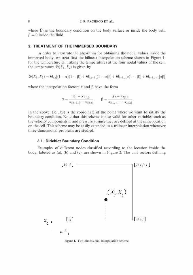
In order to illustrate the algorithm for obtaining the nodal values inside theimmersed body, we treat first the bilinear interpolation scheme shown in Figure 1,for the temperature H. Taking the temperatures at the four nodal values of the cell,the temperature HðX1;X2Þ is given by

HðX1;X2Þ ¼ Hi; j ½ð1� aÞð1� bÞ� þHi; jþ1½ð1� aÞb� þHiþ1; j½að1� bÞ� þHiþ1; jþ1½ab�

where the interpolation factors a and b have the form

a ¼X1 � x1½i; j�

x1½iþ1; j� � x1½i; j�b ¼

X2 � x2½i; j�x2½i; jþ1� � x2½i; j�

In the above, ðX1;X2Þ is the coordinate of the point where we want to satisfy theboundary condition. Note that this scheme is also valid for other variables such asthe velocity components ui and pressure p, since they are defined at the same locationon the cell. This scheme may be easily extended to a trilinear interpolation wheneverthree-dimensional problems are studied.

3.1. Dirichlet Boundary Condition

Examples of different nodes classified according to the location inside thebody, labeled as (a), (b) and (c), are shown in Figure 2. The unit vectors defining

Figure 1. Two-dimensional interpolation scheme.


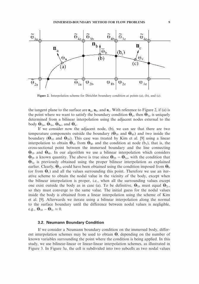
the tangent plane to the surface are na, nb, and nc. With reference to Figure 2, if (a) isthe point where we want to satisfy the boundary condition ~HHa, then �HH1a is uniquelydetermined from a bilinear interpolation using the adjacent nodes external to thebody ~HH2a, ~HH3a, ~HH4a, and �HHa.

If we consider now the adjacent node, (b), we can see that there are twotemperature components outside the boundary ( ~HH3b and ~HH4b) and two inside theboundary ( �HH1b and �HH2b). This case was treated by Kim et al. [9] using a linearinterpolation to obtain �HH1b from ~HH4b and the condition at node (b1), that is, thecross-sectional point between the immersed boundary and the line connecting�HH1b and ~HH4b. In our algorithm we use a bilinear interpolation which considers�HH2b a known quantity. The above is true since �HH2b ¼ �HH1a, with the condition that�HH1a is previously obtained using the proper bilinear interpolation as explainedearlier. Clearly, �HH1b could have been obtained using the condition imposed from �HHb

(or from �HHc) and all the values surrounding this point. Therefore we use an iter-ative scheme to obtain the nodal value in the vicinity of the body, except whenthe bilinear interpolation is proper, i.e., when all the surrounding values exceptone exist outside the body as in case (a). To be definitive, �HH1b must equal �HH2c,so they must converge to the same value. The initial guess for the nodal valuesinside the body is obtained from a linear interpolation using the scheme of Kimet al. [9]. Afterwards we iterate using a bilinear interpolation along the normalto the surface boundary until the difference between nodal values is negligible,e.g., �HH1b � �HH2c � 0.

3.2. Neumann Boundary Condition

If we consider a Neumann boundary condition on the immersed body, differ-ent interpolation schemes may be used to obtain �HH, depending on the number ofknown variables surrounding the point where the condition is being applied. In thisstudy, we use bilinear-linear or linear-linear interpolation schemes, as illustrated inFigure 3. In Figure 3a, the cell is subdivided into two subcells as two nodal values

Figure 2. Interpolation scheme for Dirichlet boundary condition at points (a), (b), and (c).


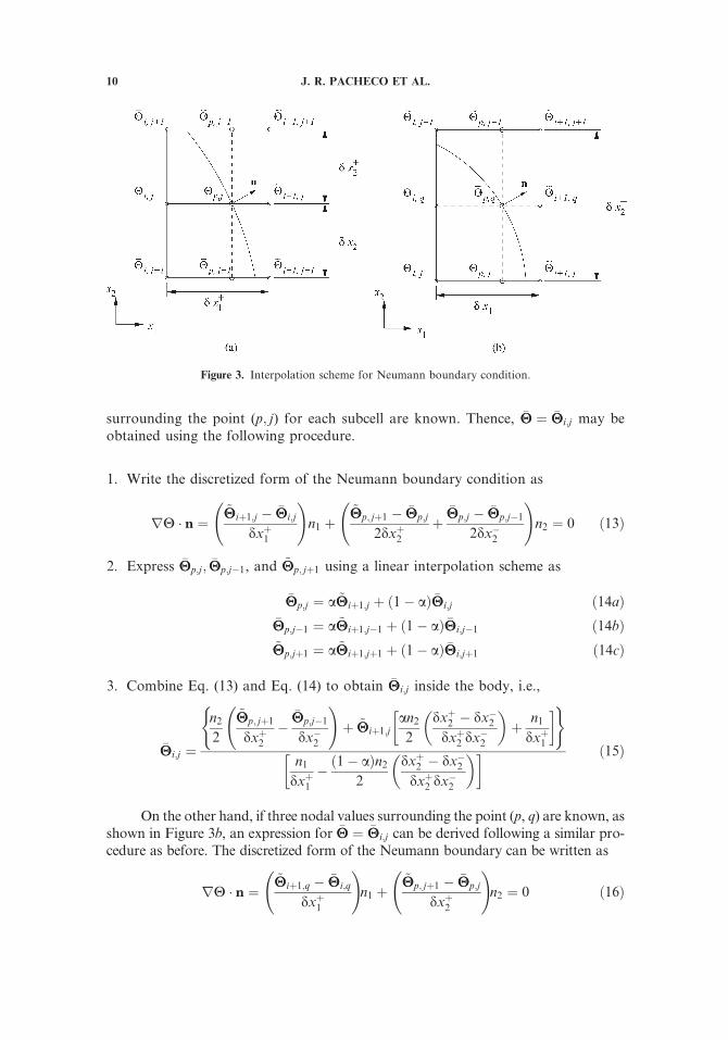
surrounding the point (p; j) for each subcell are known. Thence, �HH ¼ �HHi;j may beobtained using the following procedure.

1. Write the discretized form of the Neumann boundary condition as

rH � n ¼~HHiþ1;j � �HHi;j

dxþ1

!n1 þ

~HHp; jþ1 � �HHp;j

2dxþ2þ

�HHp;j � �HHp;j�1

2dx�2

!n2 ¼ 0 ð13Þ

2. Express �HHp;j; �HHp;j�1, and ~HHp; jþ1 using a linear interpolation scheme as

�HHp;j ¼ a ~HHiþ1;j þ ð1� aÞ �HHi;j ð14aÞ�HHp;j�1 ¼ a ~HHiþ1;j�1 þ ð1� aÞ �HHi;j�1 ð14bÞ~HHp;jþ1 ¼ a ~HHiþ1;jþ1 þ ð1� aÞ �HHi;jþ1 ð14cÞ

3. Combine Eq. (13) and Eq. (14) to obtain �HHi;j inside the body, i.e.,

�HHi;j ¼

(n22

~HHp; jþ1

dxþ2�

�HHp;j�1

dx�2

!þ ~HHiþ1;j

an22

dxþ2 � dx�2dxþ2 dx

�2

� �þ n1dxþ1

� �)

n1dxþ1

� ð1� aÞn22

dxþ2 � dx�2dxþ2 dx

�2

� �� ð15Þ

On the other hand, if three nodal values surrounding the point (p, q) are known, asshown in Figure 3b, an expression for �HH ¼ �HHi;j can be derived following a similar pro-cedure as before. The discretized form of the Neumann boundary can be written as

rH � n ¼~HHiþ1;q � �HHi;q

dxþ1

!n1 þ

~HHp; jþ1 � �HHp;j

dxþ2

!n2 ¼ 0 ð16Þ

Figure 3. Interpolation scheme for Neumann boundary condition.


We apply a linear interpolation scheme on �HHp;j; ~HHp; jþ1; �HHi;q and ~HHiþ1;q, and a bilinearinterpolation scheme on �HHp;q; that is,

�HHp;j ¼ a ~HHiþ1;j þ ð1� aÞ �HHi;j ð17aÞ~HHp; jþ1 ¼ a ~HHiþ1;jþ1 þ ð1� aÞ ~HHi;jþ1 ð17bÞ

�HHi;q ¼ b ~HHi;jþ1 þ ð1� bÞ �HHi;j ð17cÞ~HHiþ1;q ¼ b ~HHiþ1;jþ1 þ ð1� bÞ ~HHiþ1;j ð17dÞ�HHp;q ¼ ab ~HHiþ1;jþ1 þ að1� bÞ ~HHiþ1;j þ ð1� aÞb ~HHi;jþ1

þ ð1� aÞð1� bÞ �HHi;j ð17eÞ

The value for �HHi;j can now be derived by combining Eq. (16) and Eq. (17) so that

�HHi;j ¼

~HHiþ1;q � b ~HHi;jþ1

dxþ1

!n1 þ

~HHp; jþ1 � a ~HHiþ1;j

dxþ2

!n2

ð1� bÞ n1dxþ1

þ ð1� aÞ n2dxþ2

� � ð18Þ

The implementation of the boundary conditions, as described above, has been testedon several other three-dimensional problems. Computations of forced- and natural-convection heat transfer on spheres are in good agreement with published experimentalresults, and will be reported elsewhere.

4. FLUID FLOW AND HEAT TRANSFER SIMULATIONS

In order to test the proposed immersed-body formulation, we carry out simula-tions of different fluid flow and heat transfer problems. The first corresponds to thedecay of vortices, which was selected to determine the order of accuracy of themethod. The second involves an external flow in two dimensions, i.e., a circularcylinder placed in an unbounded uniform flow. The two remaining cases arebuoyancy-driven flows, selected to assess the correct implementation of the Dirichletand Neumann boundary conditions in two-dimensional domains.

4.1. Decaying Vortices

This test case is the classical two-dimensional unsteady decaying vortices prob-lem, which has the following exact solution:

u1ðx1; x2; tÞ ¼ �cosðx1Þ sinðx2Þe�2t ð19Þu2ðx1; x2; tÞ ¼ sinðx1Þ cosðx2Þe�2t ð20Þ

pðx1; x2; tÞ ¼ � 1

4½cosð2x1Þ sinð2x2Þ�e�4t ð21Þ

The governing equations for this problem are Eqs. (1)–(2) with P1 ¼ 1=Re and anegligible buoyancy force. The computations are carried out in the domain


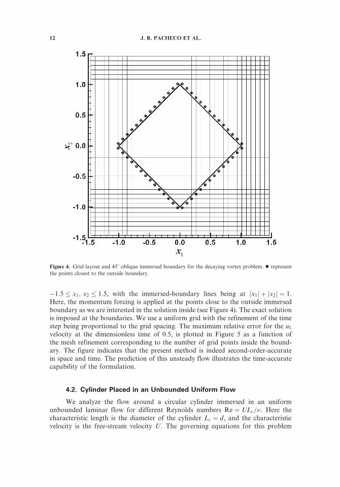
�1:5 � x1; x2 � 1:5, with the immersed-boundary lines being at jx1j þ jx2j ¼ 1.Here, the momentum forcing is applied at the points close to the outside immersedboundary as we are interested in the solution inside (see Figure 4). The exact solutionis imposed at the boundaries. We use a uniform grid with the refinement of the timestep being proportional to the grid spacing. The maximum relative error for the u1velocity at the dimensionless time of 0.5, is plotted in Figure 5 as a function ofthe mesh refinement corresponding to the number of grid points inside the bound-ary. The figure indicates that the present method is indeed second-order-accuratein space and time. The prediction of this unsteady flow illustrates the time-accuratecapability of the formulation.

4.2. Cylinder Placed in an Unbounded Uniform Flow

We analyze the flow around a circular cylinder immersed in an uniformunbounded laminar flow for different Reynolds numbers Re ¼ ULc=n. Here thecharacteristic length is the diameter of the cylinder Lc ¼ d, and the characteristicvelocity is the free-stream velocity U . The governing equations for this problem

Figure 4. Grid layout and 45� oblique immersed boundary for the decaying vortex problem. � represent

the points closest to the outside boundary.


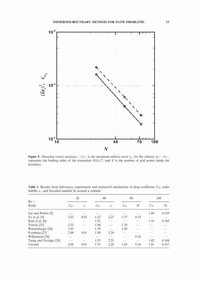
Figure 5. Decaying vortex accuracy: —&— is the maximum relative error Eu1 for the velocity u1; —�—represents the leading order of the truncation OðdxiÞ2, and N is the number of grid points inside the

boundary.

Table 1 Results from laboratory experiments and numerical simulations of drag coefficient CD, wake

bubble xc, and Strouhal number St around a cylinder

Re!20 40 80 100

Study CD xc CD xc CD St CD St

Lai and Peskin [3] — — — — — — 1.44 0.165

Ye et al. [5] 2.03 0.92 1.52 2.27 1.37 0.15 — —

Kim et al. [9] — — 1.51 — — — 1.33 0.165

Tritton [25] 2.22 — 1.48 — 1.29 — — —

Weiselsberger [26] 2.05 — 1.70 — 1.45 — — —

Fornberg [27] 2.00 0.91 1.50 2.24 — — — —

Williamson [28] — — — — — 0.16 — —

Tseng and Ferziger [29] — — 1.53 2.21 — — 1.42 0.164

Current 2.08 0.91 1.53 2.28 1.45 0.16 1.41 0.167


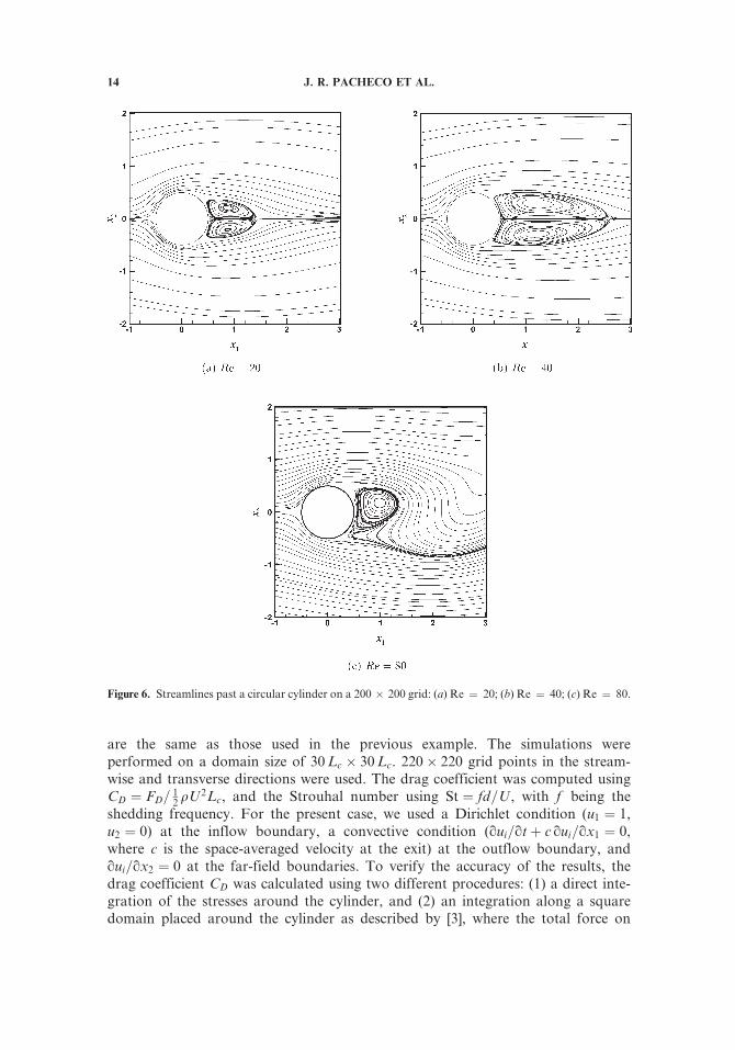
are the same as those used in the previous example. The simulations wereperformed on a domain size of 30Lc 30Lc. 220 220 grid points in the stream-wise and transverse directions were used. The drag coefficient was computed usingCD ¼ FD=

12 qU

2Lc, and the Strouhal number using St ¼ fd=U , with f being theshedding frequency. For the present case, we used a Dirichlet condition (u1 ¼ 1,u2 ¼ 0) at the inflow boundary, a convective condition (qui=qtþ c qui=qx1 ¼ 0,where c is the space-averaged velocity at the exit) at the outflow boundary, andqui=qx2 ¼ 0 at the far-field boundaries. To verify the accuracy of the results, thedrag coefficient CD was calculated using two different procedures: (1) a direct inte-gration of the stresses around the cylinder, and (2) an integration along a squaredomain placed around the cylinder as described by [3], where the total force on

Figure 6. Streamlines past a circular cylinder on a 200 200 grid: (a) Re ¼ 20; (b) Re ¼ 40; (c) Re ¼ 80.


the cylinder is given by

Fi ¼ � d

dt

ZV

qui dV �ZS

quiuj þ pdij � mquiqxj

þ qujqxi

� �� nj dS ð22Þ

In the above, m is the dynamic viscosity and V and S are the control volume andcontrol surface per unit width around the cylinder. It is to be noted that themaximum differences in the values of CD from both approaches were confinedto less than 0.1%. The results from the immersed-boundary technique suggestedhere for Re ¼ 20; 40; 80, and 100 are compared in Table 1 with those of [3, 5, 9,25–29]. The drag coefficient CD and Strouhal number St are time-averagedvalues for Re ¼ 80 and 100. It can be noted that the present results compare

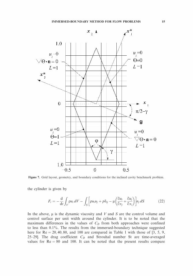
Figure 7. Grid layout, geometry, and boundary conditions for the inclined cavity benchmark problem.


quantitatively well with other numerical and laboratory experiments. Qualitativeresults are shown in Figure 6 as plots of the streamlines around the cylinder. Recir-culation regions behind the circular cylinder are shown in Figure 6 for values ofRe ¼ 20, 40, and 80. This simulation serves to demonstrate the capability of themethod to simulate separated flows.

4.3. Natural Convection in an Inclined Cavity

A standard two-dimensional enclosure consisting of two adiabatic walls andtwo walls which are heated at different temperatures, shown in Figure 7, is con-sidered next to test the numerical implementation of both Dirichlet and Neumannboundary conditions. The cavity is rotated clockwise an angle c ¼ 3p=8 between

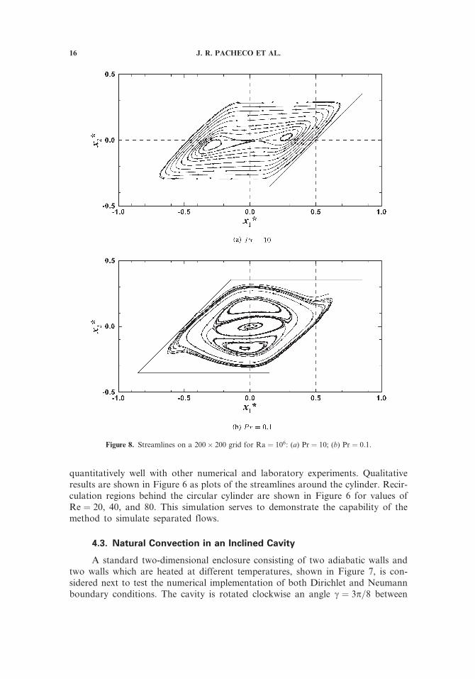
Figure 8. Streamlines on a 200 200 grid for Ra ¼ 106: (a) Pr ¼ 10; (b) Pr ¼ 0:1.


the axes x1 and x�1, with the gravity force acting along the x�2 axis. The sides of thecavity are of length L ¼ 1, and the inclination angle is u ¼ p=4. In the present casewe use Eqs. (1)–(3) with P1 ¼ Pr, P2 ¼ RaPr, and P3 ¼ 1. The computations are car-ried out in the domain �0:5 � x1 � 0:5 and �1 � x2 � 1, with the four immersed-boundary lines x2 ¼ tanðcÞ x1 cosðu=2Þ. The momentum forcing is applied atthe points close to the outside immersed boundary as we are interested in the

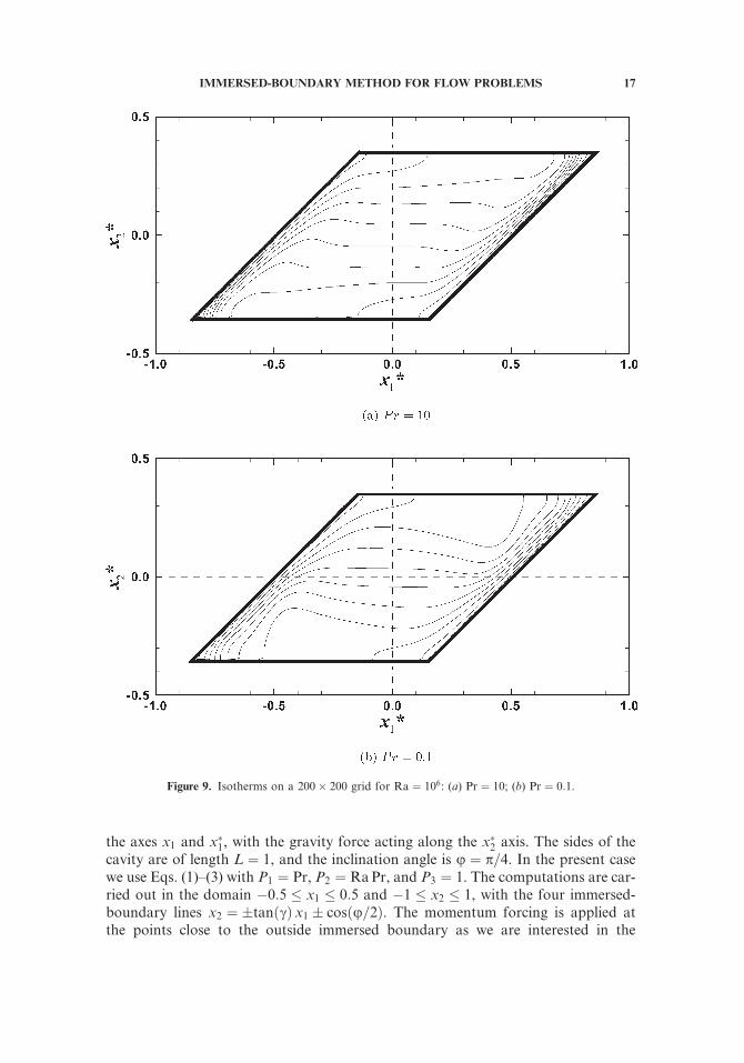
Figure 9. Isotherms on a 200 200 grid for Ra ¼ 106: (a) Pr ¼ 10; (b) Pr ¼ 0:1.


solution inside (see Figure 7). No-slip=no-penetration conditions for the velocitiesare imposed on all the boundaries, and nondimensional temperatures H ¼ 0 andH ¼ 1 are applied to the boundaries on the first and third quadrants, respectively.The walls located on the second and fourth quadrants are insulated. In this problem,flows at Ra ¼ 106 were analyzed for two values of the Prandtl number, Pr ¼ 0:1 and10, corresponding to Re ¼ 104 and 103. Our results were compared to the benchmarkresults of Demirdzic et al. [30].

The predicted streamlines for Ra ¼ 106 and Pr ¼ 10 and 0.1 are depicted inFigure 8, showing the effect of the Prandtl number on the flow pattern. In thecase of Pr ¼ 10 there is one free stagnation point located at the center of the cav-ity with no counterrotating vortices, as shown in Figure 8a. In contrast, whenPr ¼ 0:1, Figure 8b shows the presence of two free stagnation points and onecentral locus with three rotating vortices. Due to the effect of convection onthe flow, horizontal isotherms, shown in Figure 9, appear in the central regionof the cavity for the two Prandtl numbers considered. Steep gradients near the iso-thermal walls are also present. These qualitative results agree very well with thoseof Demirdzic et al. [30].

For comparison purposes, predicted Nusselt numbers along the cold wall fordifferent grid points from our method and the results of Demirdzic et al. [30] are

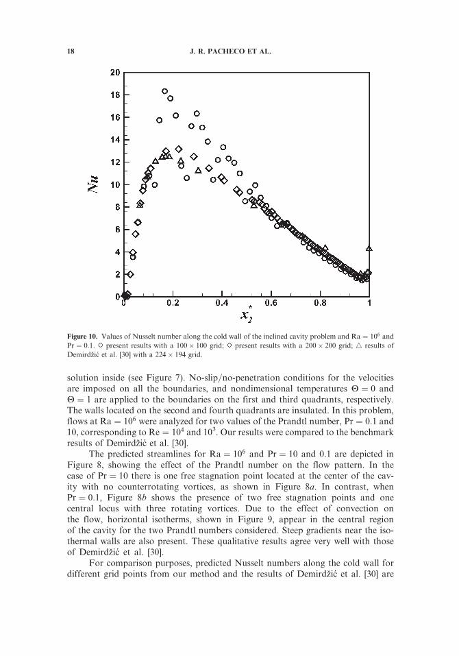
Figure 10. Values of Nusselt number along the cold wall of the inclined cavity problem and Ra ¼ 106 and

Pr ¼ 0:1. � present results with a 100 100 grid; � present results with a 200 200 grid; 4 results of

Demirdzic et al. [30] with a 224 194 grid.


shown in Figure 10 for Ra ¼ 106 and Pr ¼ 0:1. As can be observed from the figure,the Nusselt number Nu with a 100 100 grid is scattered along the wall, showingpoor convergence to the ‘‘exact result’’ of Demirdzic et al. [30]. On the other hand,there is no discernible difference between the Nusselt values obtained with a200 200 grid and the benchmark results from Demirdzic et al. [30], illustratingthe correctness in the implementation of the Neumann boundary conditions.

4.4. Cylinder Placed Eccentrically in a Square Enclosure

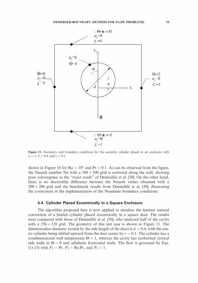
The algorithm proposed here is now applied to simulate the laminar naturalconvection of a heated cylinder placed eccentrically in a square duct. The resultswere compared with those of Demirdzic et al. [30], who analyzed half of the cavitywith a 256 128 grid. The geometry of this test case is shown in Figure 11. Thedimensionless diameter (scaled by the side length of the duct) is d ¼ 0:4, with the cen-ter cylinder being shifted upward from the duct center by E ¼ 0:1. The cylinder has anondimensional wall temperature H ¼ 1, whereas the cavity has isothermal verticalside walls at H ¼ 0 and adiabatic horizontal walls. The flow is governed by Eqs.(1)–(3) with P1 ¼ Pr, P2 ¼ RaPr, and P3 ¼ 1.

Figure 11. Geometry and boundary conditions for the eccentric cylinder placed in an enclosure with

L ¼ 1, d ¼ 0:4, and E ¼ 0:1.


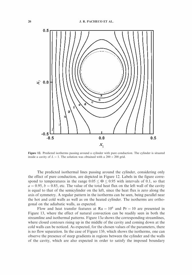
The predicted isothermal lines passing around the cylinder, considering onlythe effect of pure conduction, are depicted in Figure 12. Labels in the figure corre-spond to temperatures in the range 0:05 � H � 0:95 with intervals of 0.1, so thata ¼ 0:95, b ¼ 0:85, etc. The value of the total heat flux on the left wall of the cavityis equal to that of the semicylinder on the left, since the heat flux is zero along theaxis of symmetry. A regular pattern in the isotherms can be seen, being parallel nearthe hot and cold walls as well as on the heated cylinder. The isotherms are ortho-gonal on the adiabatic walls, as expected.

Flow and heat transfer features at Ra ¼ 106 and Pr ¼ 10 are presented inFigure 13, where the effect of natural convection can be readily seen in both thestreamline and isothermal patterns. Figure 13a shows the corresponding streamlines,where closed contours rising up in the middle of the cavity and coming down at thecold walls can be noticed. As expected, for the chosen values of the parameters, thereis no flow separation. In the case of Figure 13b, which shows the isotherms, one canobserve the presence of steep gradients in regions between the cylinder and the wallsof the cavity, which are also expected in order to satisfy the imposed boundary

Figure 12. Predicted isotherms passing around a cylinder with pure conduction. The cylinder is situated

inside a cavity of L ¼ 1. The solution was obtained with a 200 200 grid.


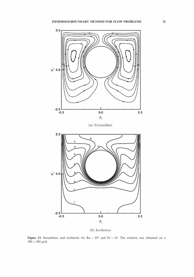
Figure 13. Streamlines and isotherms for Ra ¼ 106 and Pr ¼ 10. The solution was obtained on a

200 200 grid.


conditions and the flow conditions. All the aforementioned results agree very wellwith those reported by Demirdzic et al. [30].

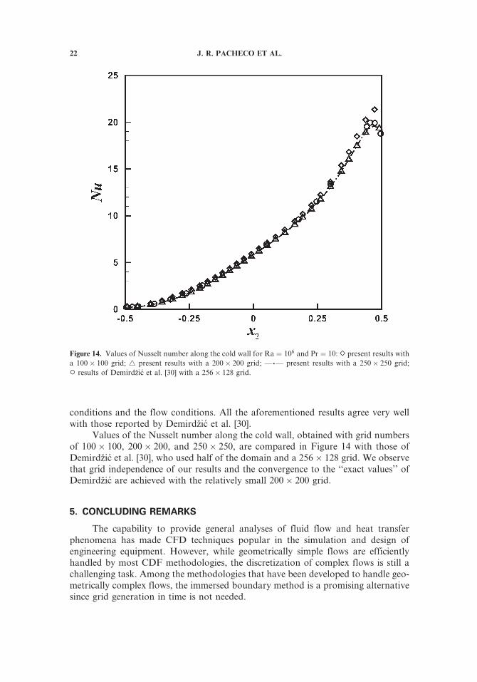
Values of the Nusselt number along the cold wall, obtained with grid numbersof 100 100, 200 200, and 250 250, are compared in Figure 14 with those ofDemirdzic et al. [30], who used half of the domain and a 256 128 grid. We observethat grid independence of our results and the convergence to the ‘‘exact values’’ ofDemirdzic are achieved with the relatively small 200 200 grid.

5. CONCLUDING REMARKS

The capability to provide general analyses of fluid flow and heat transferphenomena has made CFD techniques popular in the simulation and design ofengineering equipment. However, while geometrically simple flows are efficientlyhandled by most CDF methodologies, the discretization of complex flows is still achallenging task. Among the methodologies that have been developed to handle geo-metrically complex flows, the immersed boundary method is a promising alternativesince grid generation in time is not needed.

Figure 14. Values of Nusselt number along the cold wall for Ra ¼ 106 and Pr ¼ 10: � present results with

a 100 100 grid; 4 present results with a 200 200 grid; —�— present results with a 250 250 grid;

� results of Demirdzic et al. [30] with a 256 128 grid.


In this work, phenomenologically different problems of fluid flow and convec-tive heat transfer have been analyzed using an immersed boundary technique. Theimplementation of both Dirichlet and Neumann boundary conditions has been pre-sented in detail, and their validation has been assessed by favorable comparison withnumerical and experimental results available in the literature. The method is second-order-accurate in space and time and is capable of simulating problems of bodieswith complex boundaries on Cartesian meshes.

REFERENCES

1. C. S. Peskin, Flow Pattern around Heart Valves: A Numerical Method, J. Comput. Phys.,vol. 10, pp. 252–271, 1972.

2. C. S. Peskin, Numerical Analysis of Blood Flow in the Heart, J. Comput. Phys., vol. 25,pp. 220–252, 1977.

3. M.-C. Lai and C. S. Peskin, An Immersed Boundary Method with Formal Second-OrderAccuracy and Reduced Numerical Viscosity, J. Comput. Phys., vol. 160, pp. 705–719,2000.

4. C. S. Peskin, The Immersed Boundary Method, Acta Numer., vol. 11, pp. 479–517, 2002.5. T. Ye, R. Mittal, H. S. Udaykumar, and W. Shyy, An Accurate Cartesian Grid Method

for Viscous Incompressible Flows with Complex Immersed Boundaries, J. Comput. Phys.,vol. 156, no. 2, pp. 209–240, 1999.

6. H. S. Udaykumar, R. Mittal, and P. Rampunggoon, Interface Tracking Finite VolumeMethod for Complex Solid-Fluid Interactions on Fixed Meshes, Commun. Numer. Meth.Eng., vol. 18, pp. 89–97, 2001.

7. H. S. Udaykumar, H. Kan, W. Shyy, and R. Tran-Son-Tay, Multiphase Dynamics inArbitrary Geometries on Fixed Cartesian Grids, J. Comput. Phys., vol. 137, pp. 366–405, 1997.

8. H. S. Udaykumar, R. Mittal, and W. Shyy, Computation of Solid-Liquid Phase Fronts inthe Sharp Interface Limit on Fixed Grids. J. Comput. Phys., vol. 153, 535–574, 1999.

9. J. Kim, D. Kim, and H. Choi, An Immersed-Boundary Finite-Volume Method forSimulations of Flow in Complex Geometries. J. Comput. Phys., vol. 171, pp. 132–150,2001.

10. A. Gilmanov, F. Sotiropoulos, and E. Balaras, A General Reconstruction Algorithm forSimulating Flows with Complex 3D Immersed Boundaries on Cartesian Grids, J. Comput.Phys., vol. 191, pp. 660–669, 2003.

11. E. A. Fadlun, R. Verzicco, P. Orlandi, and J. Mohd-Yusof, Combined Immersed-Boundary Finite-Difference Methods for Three-Dimensional Complex Flow Simulations,J. Comput. Phys., vol. 161, pp. 35–60, 2000.

12. X. Wang and W. K. Liu, Extended Immersed Boundary Method Using FEM and RKPM,Comput. Meth. Appl. Mech. Eng., vol. 193, pp. 1305–1321, 2004.

13. L. Zhang, A. Gerstenberger, X. Wang, and W. K. Liu, Immersed Finite Element Method,Comput. Meth. Appl. Mech. Eng., vol. 193, pp. 2051–2067, 2004.

14. D. Goldstein, R. Handler, and L. Sirovich, Modeling a No-Slip Boundary with an Exter-nal Force Field, J. Comput. Phys., vol. 105, pp. 354–366, 1993.

15. J. Mohd-Yusof, Combined Immersed-Boundary=B-Spline Methods for Simulations ofFlow in Complex Geometries, Tech. Rep., Center for Turbulence Research, NASAAmes=Stanford University, 1997.

16. E. Balaras, Modeling Complex Boundaries Using an External Force Field on FixedCartesian Grids in Large-Eddy Simulations, Comput. Fluids, vol. 33, no. 3, pp.375–404, 2004.


17. M. Francois and W. Shyy, Computations of Drop Dynamics with the Immersed Bound-ary Method, Part 1: Numerical Algorithm and Buoyancy-Induced Effect, Numer. HeatTransfer B, vol. 44, pp. 101–118, 2003.

18. M. Francois and W. Shyy, Computations of Drop Dynamics with the ImmersedBoundary Method, Part 2: Drop Impact and Heat Transfer, Numer. Heat Transfer B,vol. 44, pp. 119–143, 2003.

19. J. Kim and H. Choi, An Immersed-Boundary Finite-Volume Method for Simulations ofHeat Transfer in Complex Geometries, Korean Soc. Mech. Eng. Int. J., vol. 18, no. 6,pp. 1026–1035, 2004.

20. Y. Zang, R. I. Street, and J. R. Koseff, A Non-staggered Grid, Fractional Step Methodfor Time Dependent Incompressible Navier-Stokes Equations in Curvilinear Coordinates,J. Comput. Phys., vol. 114, pp. 18–33, 1994.

21. B. P. Leonard, A Stable and Accurate Convective Modelling Procedure Based on Quad-ratic Upstream Interpolation, Comput. Meth. Appl. Mech. Eng., vol. 19, pp. 59–98, 1979.

22. J. R. Pacheco, On the Numerical Solution of Film and Jet Flows, Ph.D. thesis, Depart-ment of Mechanical and Aerospace Engineering, Arizona State University, Tempe, AZ,1999.

23. J. R. Pacheco and R. E. Peck, Non-staggered Grid Boundary-Fitted Coordinate Methodfor Free Surface Flows, Numer. Heat Transfer B, vol. 37, pp. 267–291, 2000.

24. J. R. Pacheco, The Solution of Viscous Incompressible Jet Flows Using Non-staggeredBoundary Fitted Coordinate Methods, Int. J. Numer. Meth. Fluids, vol. 35, pp. 71–91,2001.

25. D. J. Tritton, Experiments on the Flow Past a Circular Cylinder at Low ReynoldsNumber, J. Fluid Mech., vol. 6, pp. 547–567, 1959.

26. C. Wieselberger, New Data on the Laws of Fluid Resistance, TN 84, NACA, 1922.27. B. Fornberg, A Numerical Study of Steady Viscous Flow past a Circular Cylinder, J. Fluid

Mech., vol. 98, pp. 819–855, 1980.28. C. H. K. Williamson, Vortex Dynamics in the Cylinder Wake, Annu. Rev. Fluid Mech.,

vol. 28, pp. 477–539, 1996.29. Y. H. Tseng and J. H. Ferziger, A Ghost-Cell Immersed Boundary Method for Flow in

Complex Geometry, J. Comput. Phys., vol. 192, no. 2, pp. 593–623, 2003.30. I. Demirdzic, Z. Lilek, and M. Peric, Fluid Flow and Heat Transfer Test Problems for

Non-orthogonal Grids: Bench-Mark Solutions, Int. J. Numer. Meth. Fluids, vol. 15,pp. 329–354, 1992.


NUMERICAL SIMULATIONS OF HEAT TRANSFER AND FLUID …rpacheco/RES/PUB/nht1.pdf · NUMERICAL...

Documents

Transcript of NUMERICAL SIMULATIONS OF HEAT TRANSFER AND FLUID …rpacheco/RES/PUB/nht1.pdf · NUMERICAL...