Numerical Simulation of Viscous Filament Stretching Flows

M. S. Chandio, H. Matallah and M. F. Webster∗

Institute of non-Newtonian Fluid Mechanics, Department of Computer Science,

University of Wales Swansea, Singleton Park, Swansea, SA2 8PP, UK.

Abstract

A numerical study of the stretching of a Newtonian fluid filament is analysed. Stretching is performed between two retracting plates, moving under constant extension rate. A semi-implicit Taylor-Galerkin/pressure-correction finite element formulation is employed on variable-structure triangular meshes. Stability and accuracy of the scheme is maintained up to larger Hencky strain-levels. A non-uniform radius profile, minimum at the filament mid-plane, is observed along the filament-length at all times. We have found maintenance of a suitable mesh-aspect ratio around the mid-plane region (maximum stretch zone) to restrict early filament break-up and consequently solution divergence. As such, true transient flow evolution is traced and the numerical results bear close agreement with the literature. Key words: Taylor-Galerkin, filament-stretching, viscous, free-surface. 1. Introduction

Flows with significant elongational components are common in industrial applications, such as in fibre spinning. The same applies within some rheological instruments, as typified under the measurement of extensional viscosity. The most common types of extensional flow instabilities that occur are necking, capillary and filament break-up. In fact, filament-stretching flows are common in everyday-life, and may be used as a technique to measure extensional viscosity in highly mobile fluids, where extension rates may be large. Currently, the filament stretching extensional rheometer (FSR) has emerged as a controllable device, for such purposes. Matta and Tytus [13] were the first to introduce such a device. A modern form has been developed by Tirtaatmadja and Sridhar [14] for low-viscosity liquids. In recent years, due to the development of filament stretching rheometers, attention has been

∗ author for correspondence email: M.F.Webster@swan.ac.uk

2

diverted into this new area, and on to the measurement of extensional properties of polymer solutions and melts. Yao et al. [4-5], Sizaire & Legat [3] and Gaudet & McKinley [10] have performed numerical simulations, based on the filament stretching rheometer of Tirtaatmadja & Sridhar. Experimental studies were reported in Yao et al. [5] and by Spiegelberg et al. [6-7]. Major attention has been focused on the analysis and comparison of the fluid kinematic and dynamic evolution of the extensional stresses in these liquid bridges. Both Newtonian and viscoelastic fluids have been considered. In the literature, little has been reported numerically, based on the FSR of Tirtaatmadja and Sridhar [14]. Numerical solutions have been restricted largely to small deformations [4]. In the present work, we discuss in some detail the numerical difficulties that arise during the simulation of elongation in liquid bridges. We, consider the validity of these techniques whilst calculating extensional viscosity. First, a brief literature review is presented, covering the extensional deformation histories observed.

Matta and Tytus [13] investigated constant force experiments, allowing the lower-plate, that grips the fluid, to fall under gravity. In such circumstances, these authors showed that liquid bridge experienced constant uniform extension when the plates moved apart rapidly. Tirtaatmadja and Sridhar [14] considered a variation to the stretching procedure for mobile polymer systems. In their work, the plates were moved apart at an exponential retraction-rate, so as to impose constant stretch-rate at the centre of the filament. Berg et al. [18] were the first to conduct experimental tests on a reducing diameter device (RDD). The diameter of the end-plates, in such devices, is reduced at an exponential rate with filament elongation. This type of device exhibits homogenous flow kinematics in the liquid bridge at low Hencky-strains (ε=1.4). However, it has proved practically difficult to investigate the extensional properties of liquid bridges using the RDD, due to mechanical design constraints.

Yao and McKinley [4] conducted a numerical study to investigate the transient response of Newtonian and viscoelastic liquid bridges. A commercial finite element package (POLYFLOW) was employed in their simulations, using 9-node quadratic, quadrilateral elements. An elliptic mapping and remeshing technique (see Thompson [21]) was introduced to redistribute the internal nodes, according to the displacement of the moving boundaries. This was found helpful in avoiding excessive mesh distortion. Their findings were based upon the Reducing Diameter Device (RDD) of Berg et al. [18] and a velocity compensation technique, as proposed by Tirtaatmadja and Sridhar [14]. The spatial and temporal non-homogeneity of the fluid kinematics and viscoelastic stress were investigated in some considerable detail. The transient response for Newtonian fluids was compared against that for some viscoelastic fluids. Yao and McKinley argue that accurate extensional material properties cannot be based on net experimental tensile force measurements, due to inherent inhomogenity of deformation within the filament. A RDD approach is

3

commended as being optimal to improve homogeneity in flow kinematics. Sizaire and Legat [3] conducted a similar numerical study to that of Yao and McKinley [4]. Sizaire and Legat neglected the effects of gravity and inertia and reasonable agreement was reached in comparison to the literature. Indeed, the velocity compensation technique [14] may simplify the calculation of extensional viscosity. In contrast, the stress field developed within the filament may remain far from homogenous [6]. In our investigation, we have relied upon a direct approach instead of a compensation technique. The magnitude of the resultant strain-rates is observed at the filament mid-plane, as a function of Hencky-strain. Flow kinematics, resultant force on the plate, and extensional viscosity are each computed and compared against published results.

Gaudet et al. [9-10] analysed numerically the transient evolution of free-surface shape and applied force on the plates for Newtonian liquid bridges. In their work, the plates moved apart at a constant, prescribed velocity. Deformation patterns and liquid-bridge break-up time, for materials of different viscosities, were investigated using a boundary integral method. In their subsequent work, Gaudet and McKinley [10] introduced a viscoelastic liquid-bridge to simulate the extensional dynamics of stretching filaments for constant viscosity Boger fluids. Such fluids were represented conveniently by Oldroyd-B type models. Predictions were compared for low Hencky strains to their experimental results and found to lie in close agreement.

Further reference may be found in Kolte and Szabo [12], who analysed the capillary thinning of filaments for Newtonian and viscoelastic fluids, both experimentally and numerically. Here, a new instrument design was introduced, the liquid filament rheometer (LFR). The top-plate of this new device was fixed and the bottom-plate was attached to a moving-bar. When released, the bar and the bottom-plate fall under gravity. Minimum filament radius was recorded directly, capturing visual images on videotape, to be compared against numerical predictions. Hassagar et al. [8] have investigated the occurrence of ductile failure for Newtonian and viscoelastic fluid samples without surface tension. These authors employed a Lagrangian finite element procedure, and hence demonstrated that Newtonian liquid bridges do not show ductile failure in the absence of surface tension. However, a mixed response (stability and ductile failure) was gathered for viscoelastic fluids. In addition, Ainser et al. [20] performed simulations for the extension of viscoelastic samples, under the weight of a falling body. Once more, a Lagrangian finite element approach was applied with a multi-mode PTT model. The flow characteristics were found to be sensitive to variation in model parameters. To avoid excess mesh distortion at protracted extension lengths, periodically these authors regenerated a fresh mesh (involving solution re-projection). A similar strategy is implemented in our own present studies.

Here, a semi-implicit Taylor-Galerkin/Pressure-Correction (SITpac) finite element method [1-2] is used to model the stretching and break-up of Newtonian

4

liquid bridges. We have used the material parameters proposed by Sizaire and Legat [3], identified by McKinley on the basis of steady-shear data, see Table 1. Principal interest lies in quantifying solution evolution through various Hencky strains (thus, through time). Plates are retracted at an exponential rate, to provide a constant stretch-rate at the filament mid-plane. The present work presumes axi-symmetry, and symmetry about the horizontal mid-plane between the flat-plates. Elsewhere, when considering viscoelastic fluids, we have found it an effective strategy to take the full filament length, hence avoiding excessive discretisation errors about the filament mid-plane. This is particularly important in the viscoelastic counterpart problem, as there flow kinematics and stress enters the problem in a direct manner. Both influences of inertia and gravity may be neglected. The complexity of the problem lies in the dominating presence of deforming free-surface boundaries. To determine the eventual position of the free-surface, both dynamic and kinematic conditions must be imposed on such boundaries.

Our approach has been to devise algorithms that demonstrate accuracy, stability and consistency, throughout the transient stretching process. In the present study, we have recourse to refer extensively to the fundamental work of Yao and McKinley [4] and Sizaire and Legat [3]. To avoid temporal mesh distortion and to maintain smooth and consistent nodal distribution, an efficient remeshing algorithm is invoked at each time-step, see on. 2. Governing equations

For incompressible, isothermal laminar flows, the governing equations may be described through the system comprising of the momentum and the continuity equations. In the absence of body forces, these may be expressed in the form

. . pt

∂ρ = ∇ − ρ ∇ − ∇∂u

T u u (1)

∇.u = 0 (2) where independent variables are time, t, and space, x. Dependent field variables are fluid velocity, u(x,t), and isotropic pressure, p. Material density is ρ. For Newtonian flows, the stress T is defined via a Newtonian viscosity µ0, and the rate-of-deformation tensor D, and velocity gradient L, as Τ = 2µ0D (3) where

t

tL L and L u

2

+= = ∇D . (4)

5

With a constant viscosity µ0 and using the continuity equation (2), the

celebrated Navier-Stokes equation can be recovered:

2 . pt

∂ρ = ∇ − ρ ∇ − ∇∂u

u u uo (5)

where 2u0µ ∇ is the diffusion term.

For the dimensionless variables x*, u*, t*, and p*, we have chosen to scale by

x=x*L0, u= 0εg

L0u*, t = t*/ 0ε

g

, p = p* 0 0εg

, where L0 is the initial length of the fluid

filament and 0εg

is the initial imposed stretch-rate. Hence, we may define an equivalent non-dimensional system of equations to (1)-(2) discarding the * notation for convenience of representation,

pt

∇−∇−∇=∂∂

u.uReuu

Re 2 ,

.u 0∇ = . (6)

where the non-dimensional group Reynolds number is defines a 20

0

ρε=µ

g

LRe

3. Finite element analysis

A time-dependent Taylor-Galerkin/Presseure-Correction algorithm (SITpak) [1,2] is used to solve the governing equations (6). This involves a two-step Lax-Wendroff approach, based on a Taylor series expansion up to second order in time, to compute solutions through a time stepping procedure. A two-step pressure-correction method is applied to handle the incompressibility constraint. Employing a Crank-Nicolson treatment on diffusion terms produces an equation system of three fractional-staged equations [1,2]. In stage one a non-solenodal velocity field un+½ and u* are computed via a predictor-corrector doublet. The resulting mass-matrix bound equation is solved via Jacobi iteration. With the use of u*, the second stage computes the pressure difference, pn+1-pn, via a Poisson equation, and the application of a direct Choleski solver. The third stage completes the time step loop, calculating the end-of-time-step solenoidal velocity field un+1, again by a Jacobi iterative solver. The details upon this implementation may be found in [1,2].

Following the notation of Cuvelier et al. [24], the velocity and pressure fields are approximated by U(x,t) = Uj(t)φj(x) and P(x,t) = Pk(t) ψk(x), where U and P

6

represents the vectors of nodal values of velocity and pressure, respectively, and φj are piecewise quadratic and ψk linear basis functions.

The fully-discrete semi-implicit Taylor-Galerkin/pressure-correction system of equations may be expressed in matrix form as,

Stage 1a 1

22 Re 1( )( ) [ Re ( )]

2

n n T nM S U U S N U U L P Ft

++ + = − + + +

∆

Stage 1b 1

* 2Re 1( )( ) ( [ ] [Re ( ) ]

2

nn T nM S U U SU L P N U U Ft

++ − = − + − +

∆

Stage 2 n 1 n *2ReK(P P ) LU

t+ − = −

∆

Stage 3 n 1 * T n 1 nRe 1M(U U ) L (P P )

t 2+ +− = −

∆, (7)

where M, S, N(U), L, and K are consistent mass matrix, momentum diffusion matrix, convection matrix, pressure gradient matrix and pressure stiffness matrix, respectively. With elemental fluid area dΩ, such matrix notation implies,

,

( ) ( ) ,

(( ) ) ,

,

,

φ φ

φ φφ φ φ

φ

ψ ψ

φ φ

Ω

Ω

Ω

Ω

Ω

= Ω

∂ ∂= + Ω

∂ ∂∂

= Ω∂

= ∇ ∇ Ω

= ∇ ∇ Ω

∫

∫

∫

∫

∫

ij i j

j jij i l l l l

jk ij

k

ij i j

ij i j

M d

N U U U dx y

L dx

K d

S d

.dgF 2i

2

2i Γφ= ∫Γ

(8)

4. Problem description

We consider the case of a cylindrical filament of Newtonian fluid, stretched in time from a rest state, see fig.1. This procedure is termed ‘filament-stretching’, and is of interest in several manufacturing processes, in particular, within the printing and foods processing industries. This problem has been the object of numerous

7

experimental and numerical investigations [3-20], as discussed above, and provides a wealth of data for comparison purposes.

In an ideal, homogeneous uniaxial elongational flow, a liquid bridge of initial length L0 is stretched at an exponential rate, so that the filament length (similarly, distance separating any two material elements), at any particular time t, is given by:

),texp(LL 00t

•ε= (9)

where 0

•ε is an imposed initial stretch-rate. In this ideal state and at any moment in

time, the radius of the filament remains uniform throughout its length, and decreases from its initial value following the functional representation,

).2

texp(RR

0

0t

•ε−= (10)

For pure-extensional uniaxial flows, the axial and radial velocity components

are described, viz:

zU 0z

•ε= and .r

2

1U 0r

•ε= (11)

The extensional viscosity, µe, is defined via the tensile-stress growth in the

fluid, as a function of the imposed-extension rate in the liquid bridge. This may be expressed in form

,)t,(0

rrzz0e •

•

ε

τ−τ=εµ (12)

where, τzz and τrr are the normal components of extra-stress τ, defined as

τ = τs + τp. (13)

Here, τs and τp are solvent and polymeric contributions to the extra-stress, respectively. For Newtonian flows, we have simply,

τ = τs = 2 µ0 D. (14) For a Newtonian fluid with steady shear-viscosity µ0, extensional viscosity

can be represented as e 03µ = µ [22].

8

In the absence of gravity and inertia, the tensile-force acting on any cross- sectional of filament of uniform radius R, can be obtained by integrating the normal stress differences (τzz- τrr), over that area. Thus, over the circular area of the plate, this leads to the identity,

2

zz rrF R ( )= π τ − τ . (15) Hence, via equation (12), the extensional viscosity can be expressed in terms

of applied normal force,

.R

F)(

02

0e •

•

επ=εµ (16)

As a consequence, the transient Trouton ratio can be realised, through the

ratio of extensional to steady shear-viscosity,

e

0

Trµ=µ

. (17)

In the present study, we restrict attention to Newtonian fluids, and the set of

operating conditions recorded in [3], see Table 1. We recognize that the flow generated in the filament stretching configuration, as shown in fig.1, is neither ideal nor uniaxial, due to boundary influence. Here, we attempt to reproduce uniaxial elongation by separating end-plates at a prescribed increasing velocity. The main

interest lies in Hencky-strain,

=ε=ε

•

0

0L

)t(Llnt , as a function of time, where L(t) is

the length of the whole filament (distance between two plates) at time t, and L0=L(0) is the initial sample length. Plates are retracted at an exponential-rate, by arranging that

).texp(2

L)t(L 0

0•ε= (18)

9

ρ (density) 890 (kg m-3)

0

•ε (stretch-rate) 1.6 (s-1)

L0 (initial length) 2.0 10-3 (m)

R0 (initial radius) 3.5 10-3 (m)

χ(surface-tension coefficient) 28.9 10-3 (m)

µ0(Newtonian shear viscosity) 98 Pa s

Table 1. Sample material properties

The geometry (one quarter of domain) and the boundary conditions are provided in fig.2. On the moving-plate, a driving velocity is imposed of:

)texp(2

L)t(U 0

00

z

••

εε= , Ur (t) = 0. (19)

The presence of non-deforming rigid end-plates and no-slip boundary

conditions, induces an additional shear-component to the flow, that develops locally to the end-plates. This will subsequently contribute to the deformation history. 5. Free surface computation and boundary conditions

A complete definition of the problem requires appropriate boundary conditions. Dirichlet type boundary conditions are imposed on the known parts of the boundary. Continuity of normal and tangential velocities is applied at a fluid-solid interface and continuity of stress at a free-surface [25]. On the free boundary Γfs, considering an appropriate amount of surface-tension, we impose the following dynamic and kinematic boundary conditions as described below: 5.1 Dynamic boundary condition 1 1

ext 1 2. (p (R R )).− −= − + χ +n nσ (20)

where σ is the Newtonian Cauchy-stress tensor, defined as: ij ij 0 ij(p 2 d )σ = − δ + µ . (21)

10

Here, χ, n , d and pext are the surface tension coefficient, outward unit normal

vector to the boundary fs∂Γ , rate-of-deformation tensor and atmospheric pressure,

respectively. R1 and R2 are the principal radii of curvature of the interface, defined functionally as

,

z

hz

h1

R

2

2

2

1

∂∂

∂∂+

= 2/1

2 z

h1hR

∂∂+−= (22)

In the axisymmetric case we must consider two radii of curvature with opposite effect [26]. 5.2 Kinematic boundary condition

In order to find the eventual position of the free-surface, we use

,r z

h hu u t

t z

∂ ∂= − ∀∂ ∂

. (23)

If the free-surface is flat (vertical and normal to the horizontal), at the outset of the simulation, it will be driven by radial-velocity alone. This is always the case near the filament mid-plane, where we have,

r

h h0; and u

z t

∂ ∂= =∂ ∂

. (24)

Elsewhere, equation (23) applies.

Due to the underpinning boundary conditions at the interface of the rigid end-plate and free-surface, the second term on the r.h.s. of equation (23) stimulates instabilities on the free-surface (oscillations in profile, prominent in the first few elements, near the moving-plate), see fig. 4. Since, these instabilities are local to the plate and free-surface region, a Crank-Nicolson treatment (with θ = 0.5) is introduced in discretising the second-term of r.h.s. of equation (23). With θ =1, equation (23) is recovered, under as explicit, one-backstep interpretation between tn+1 and tn. This is a measure taken to circumvent such numerical shortcomings, implemented as

11

∂∂−

∂∂θ+

∂∂−=

∂∂

−−+ 1nn1n1n ttttz

tr

t

z

h

z

h

z

huu

t

h (25)

where 0 ≤ θ ≤1.

The use of equation (25) introduces smoothness and consistency in surface profiles; see fig.5, at no serious additional run-time cost. In this manner, an attempt has been made to avoid using an extra solver (a conventional approach) to correct free-surface instabilities.

5.3 Conservation of mass

Since the flow is incompressible, the free-surface location must satisfy the constraint that the volume of liquid remains constant, viz

L 2

L(z)dzV R

−= π∫ . (26)

Satisfaction of this condition, at specific times of filament evolution, is ensured at Algorithm, step 6 (see below). 6. Remeshing strategies

The choice of mesh is a crucial and important step in simulating any flow problem. Successful implementation of the numerical algorithm will depend in part upon the accuracy afforded by the mesh. It is conspicuous that the initial mesh will deform axially, in time, due to axial stretching and radially due to the pinning boundary conditions and the presence of the free-surface. In order to avoid mesh distortion, a strong remeshing rule* is needed to distribute the internal, as well as boundary nodes, in such a fashion as to maintain solution smoothness and stability up to higher levels of Hencky-strain. Two different methods are commonly employed to achieve this goal: (i) fixed-connectivity approach; and (ii) automatic (adaptive)-mesh generation. The fixed-connectivity approach will maintain the original sparsity pattern, associated with the matrices of the discrete equations. Distribution of interior nodes is made by a predetermined rule, using logarithmic, tan-hyperbolic (tanh), or uniform remeshing transformations. A second approach, used in recent years, is automatic mesh regeneration, particularly suitable for domains of arbitrary shape. This is achieved either by removing or inserting new elements until the mesh has

* A remeshing strategy that possess the ability to maintain element density (mesh concentration), as well as mesh aspect ratio, near the point or line of reference, without adding/removing new elements.

12

acquired the desired nodal density in each region of the domain. Such an approach is most useful when the problem domain is significantly changed, due to large surface-tension effects. At relatively small deformation, the cost of generating new elements/nodes is low. However, under large deformation, as presently, this scheme is not cost-effective. It necessitates a full restart of any time-integration scheme involved, incurring large expense. The projection of solution (interpolation of primitive variables), implies considerable cost and introduces degradation in accuracy. To circumvent such difficulties, we have allotted to employ a fixed-connectivity approach. A fresh mesh is generated periodically in time (specific Hencky-strains, equating to excessive mesh distortion) and the solution is reprojected from the previous mesh to the new mesh. With a single mesh (M1), we are able to retain stability up to Hencky-strain levels of 4.8+. Nevertheless, a new mesh (M2) is deemed necessary at Hencky strain ε = 2.56 to capture accuracy on the field, up to higher Hencky-strain levels of (ε = 3.52+). Each is discussed in subsequent sections below.

The kinematic iteration is a natural, separate solution stage for transient free- surface problems. From some initial flow field and domain, the free-surface and moving-boundary is advanced, according to the flow on such boundaries. An updated flow field is calculated and the boundaries advance once more, consecutively. At each step the mesh is adjusted so as to comply with kinematic conditions, (25), that match the motion of the moving boundaries to the velocity field. The kinematic iteration can be applied to solve a fully transient problem, or simply to solve a steady state problem. Due to the underpinning boundary conditions and the presence of the free surface, the mesh experiences large deformation both radially (near the interface of the free-surface and the top-plate) and axially. Uniform remeshing is performed radially. For axial remeshing, where the mesh undergoes large stretching, two different remeshing techniques, tan-hyperbolic (tanh) and logarithmic remeshing rules have been implemented. The principal objective is to maintain smoothness of the mesh, in such a manner, that the nodes remain concentrated in certain regions of reference. Redistribution of mesh points and mesh concentration in the tanh-scheme are maintained by a specified control parameter (for more details, the reader is referred to implementation of elliptic-mappings, see Thompson et al. [21]). A typical such mapping function may be expressed as:

,tanh

)H1(tanh(1H

n

1ntit

i β−β−=

+

(27)

where, Hi, i0 H 1,≤ ≤ is axial node-position of node i, and β is a mesh-density

control-parameter.

13

With the tanh-scheme, large aspect-ratios have resulted about the mesh mid-plane region. This causes filament break-up away from the mid-plane, at large Hencky-strain levels, see fig.7. Nevertheless, this scheme performs well at relatively small Hencky-strain levels. Since the problem under consideration, does experience large deformation, a log-remeshing algorithm is employed instead [21]. Since the shape of the free-surface is highly curved near the top moving-plate, so there, a finer mesh is deemed necessary to retain mesh aspect-ratio, and hence accuracy and stability. A modified log-remeshing approach is implemented for axial remeshing, where the mesh undergoes large stretching. This mapping function is given by

n 1tn 1 nt t

i i2i H

H Htelm(telm 1)

++ ∆= +

+ (28)

where, telm is the total number of elements along the mesh-length, and n 1t

iH+

∆ is the

current displacement. In this manner and by design, high element-density is maintained near the top-plate, see contrast in results between fig.7 and fig.8.

Two rectangular meshes M1 of 12 x 40 elements, with 2025 nodes and 960 triangular elements, and M2 of 12 x 106 elements, consisting 5025 nodes and 2544 triangular elements, are used to perform the numerical simulation. The simulation commences from a simple mesh, but soon encounters large deformation that persists in time due to the transient nature of the problem. To avoid excessive mesh distortion at large deformation, and to retain smooth internal node distribution, the above cited low-cost remeshing algorithm (28) is applied at each time-step. Results are compared with Sizaire and Legat [3], Yao and McKinley [4] and Gaudet and McKinley [10]. Our solutions prove stable up to large Hencky-strains of 4.8+ units. A high level of field solution accuracy is maintained and reported, up to Hencky-strains of 3.52+ units. This exceeds findings in the literature.

With respect to mesh-structure, it has been found advantageous to introduce a slight modification in the corner elements of these meshes. In fig.6.a, a schematic diagram of the initial mesh-orientation is illustrated. Here, node N2 and N4 are surrounded by two elements. In order to compute velocity gradients at node Ni, we have recourse to a recovery technique [25], that takes the average of values from surrounding elements.

Velocity gradients can be expressed in the form:

ek

k

G ( , t) ( , t)x

∂=∂

ux x , where k =1,2 (29)

14

Approximating the velocity vector, u(x,t) by finite element interpolation on each element gives uh:

)t(u)x()t,(uN

1jjj

h ∑=

φ=x (30)

where N represents the number of nodes per element. By combining equations (29) and (30), a direct calculation of the velocity gradients is possible thus:

)t(ux

)x()t,(G j

N

1j k

jh,ek ∑

= ∂φ∂

=x . (31)

Equation (31) yields nodal gradients per element. Straight averaging over

elements for each nodal-value, generates unique values, around which the quadratic continuous interpolation is based. For more details, the reader is referred to Matallah [25].

For an incompressible fluid, from the no-slip boundary conditions and continuity equation, we have Drr= Dzz= 0 on end-plates. Through application of a recovery technique [25], corner-nodes N2 and N4, as shown in fig6.a, would gather contributions from more than one boundary element, To avoid this, we can use either a pointwise finite-difference approach on the boundaries, or adjust the element topology in that region, so that, only a single element contributes to the node. Note that nodes N1 and N3 receive contributions from a single element only. In the present simulations, we have allotted for mesh-orientation, as shown in fig.6.b, with the use of one-dimensional point-wise approximation+ over straight-line boundaries, Γplate, Γcl and Γmid-plane, see fig.6.b. We have found that point-wise approximation on the free-surface boundary (Γfs) performs less well. Hence, we have taken recovered velocity-gradients [25], upon the deformed free-surface boundary and internal field. Within the purely viscous scenario, the rate-of-deformation tensor only enters the calculation through a post-processing operation. However, for complex free-surface viscoelastic flows, where gradients play an important role in the calculation of primary-variable stress fields, the precise details on velocity gradient estimation are crucial. There, both mesh-structure and velocity-gradient estimation must be revisited.

+ This still appeals to the underlying fe-interpolants, but at selected sample points and along restricted directions.

15

7. Algorithm

The individual sequence of steps taken within a single Hencky-strain step (∆tHencky) are identified as follows:

1. Hencky-strain, time-step number: nstep=nstep+1 2. Fix plate-boundary conditions via equation (19) 3. Move plate via equation (18) (∆tHencky) 4. Update mesh-points locations, to occupy new position relative to

plate-movement, via equation (28) 5. Correct velocity and pressure fields solving fractional-stages (7),

with dynamic boundary condition (20), to reach convergence tolerance 1.0E-05, (∆tinner)

6. Compute free-surface via equation (25), (∆tfs) (i) update mesh-points radially; (ii) compute volume; via equation (26); if ||Volexact-Vol.h||/ ||Volexact || <= 1.0E-03 goto 8; continue (iii) solve fractional-stages (7) to update-solution (iv) Goto 7

7. Print output: normal force, extension-rate, Trouton ratio, Rmin 8. Print solution at current Hencky-strain level (real-time) 9. Goto 2

In the current formulation, we choose three different time-step sizes as

∆tHencky to shift the plate at each Hencky-strain (real-time, step 3), ∆tinner to compute the velocity field (step 5) and ∆tfs for free-surface movement. For mesh M1, up to Hencky-strain levels ε=2.56, we have taken ∆tHencky=∆tinner. For mesh M2, at smaller mesh-size, we have used ∆tinner=∆tHencky* 0.5 and for free-surface computation, taken ∆tfs= ∆tinner* 0.5.

Since, the flow under consideration is incompressible, so the volume of the liquid-bridge must remain constant throughout the stretching period. This check is performed at step 6 of the above algorithm. At each ∆tfs, the free-surface boundary is moved using (25) in such a manner that the relative error norm between the exact volume (volexact initial volume) and the computed volume (volh) remains less than a specified tolerance (say, 1%-2% of initial volume). 8. Numerical results and discussion

A half-length model, see fig.2, is considered for simulation at a negligible Reynolds number. The volume of the liquid bridge is conserved at all times using equation (26). The deformation of the filament and its free-surface evolution is

16

depicted in fig.8, at various Hencky strain levels. Everywhere, the radius varies along the filament, at all times, due to the underpinning boundary conditions on the moving end-plate. This results in large deformation during stretching. Minimum radius is computed at the midpoint, see fig.9. It can be seen that the slope of minimum radius, Rmin, decreases in a smooth exponential fashion, equation (10), up to a Hencky-strain level of ε = 2.0. Later, a slight departure is observed that continues up to the break-up of filament (ε=4.8+) using mesh M1. Though, an acceptable minimum radius profile is achieved up to Hencky strain level of ε = 4.8+, this setting failed to capture accuracy in other variables of interest, for example, in flow kinematics, strain-rates and extensional viscosity distributions. This is due to high deformation in the middle of the fluid column, where mesh elements have experienced a large aspect ratio. Hence, a new mesh (M2) is generated and simulation recommenced. With this new mesh, we have been able to capture accuracy in flow kinematics and other variables of interest, but failed to control the exponential behaviour of Rmin. It is shown in fig.9, that the filament, becomes dramatically thin suddenly in the symmetry plane for Hencky strains of ε = 3.2+. This subsequently causes filament break-up at ε = 3.52+. These instabilities can be attributed to the rapid increase in radial flow kinematics and high extension-rates generated at the midpoint, which differ from the imposed constant extension-rates. These are discussed in detail below.

For an ideal uniaxial flow, the radial and axial velocity profiles can be obtained using equation (11). For flows, which are not purely uniaxial, Spiegelberg et al. [6] have proposed a lubrication theory solution (hereby referred to as analytical solution) for viscous Newtonian fluids. This approximation is true for small Hencky-strain levels. Hence, we have compared our computed radial and axial velocity profiles with this solution, described by

,L

z

L

z13U

pp

0r

−ε−=

• (32)

.L

z

L

z23rLU

pp

pz

−−=

• (33)

The comparison of the complete numerical solution with that represented by (32) and (33) demonstrates the accuracy of radial and axial velocity profiles at small Hencky-strains, see figs.10-13. Axial velocity profiles are calculated along the centreline r=0 and the radial velocity profiles, Ur, on the deformed free-surface. Our results are in close proximity with the analytical solution (lubrication approximation) [6] up to Hencky-strains ε = 2.56+. A slight deviation is observed from the lubrication

17

solution after Hencky strain level of ε=2.56, see fig.12, ε=2.88. With the new mesh M2, we have been able to recapture the accuracy up to Hencky strain level of ε=3.52. There, radial velocity, Ur, has attained larger values and subsequently causes the thinning, and ultimate break-up of the liquid-bridge, see fig.13. It is observed here that, large radial displacements are obtained at the mid-plane symmetry due to the high radial velocity in that region. Colour contours of both radial and axial velocity components are shown in fig.14 and fig.15, respectively. Parabolic profiles of radial velocity component are obtained in the liquid bridge. The axial velocity component has exposed uniformity across the filament and non-homogeneity along the length of the liquid-bridge, maximum on the plate and vanishing on the mid-symmetry plane. The radial velocity** is observed to be the major driving factor. It is responsible for the correct free-surface profile, and assists in retaining solution accuracy and stability at large Hencky-strains. Our results are in close agreement with those of Yao and McKinley [4], with velocity correction results up to Hencky strain levels of 3.0 units and with Sizaire and Legat [3] up to Hencky strain levels of ε = 3.52+.

Another important quantity, difficult to estimate experimentally, is the history of the rate-of-deformation within the liquid bridge. In an ideal uniaxial flow, the rate-of-deformation tensor satisfies equation (11) at all times. Thus, a shear-free flow field

is obtained as Drz = 0 and 0zzD•ε= . The flow under consideration inherits shearing

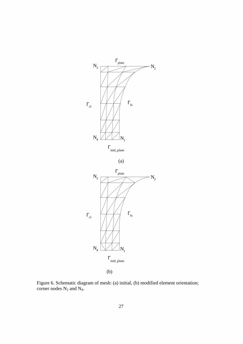
components due to the no-slip boundary conditions. The colour contours of Drz and Dzz components of the rate-of-deformation tensor are shown in figs.17-18. Initially (at small Hencky-strains) the flow in the liquid-bridge is dominated by its radial velocity component (moving inward). Consequently, some shear arises due to the underpinning boundary conditions, prior to the development of dominant extension in the flow. Hence, significant shearing effects can be observed at small Hencky-strain levels of ε = 0.32 in the fluid filament. Maxima in Drz are at the interface of the free-surface and the rigid end-plate. These shearing effects, decline with increasing Hencky-strain levels, see fig.17. Equivalently, maxima in Dzz are observed at the mid-plane.

Fig.9 demonstrates that the minimum filament radius, Rmin(t), beyond Hencky-strain levels of ε = 2.0 decrease in a complicated fashion, due to the presence of the no-slip boundary condition. As a result, strain-rates vary both in space and time. Consequently, analysis of results becomes complicated and does not lead to true material properties [14]. Since the flow near the mid-plane is almost shear-free, Kroger et al. [17] and Spiegelberg et al. [6] proposed a method to compute, transient extensional viscosity, based on an effective deformation-rate:

** Free-surface movement largely depends upon Ur. The larger the Ur (magnitude), the smaller the Rmid(t).

Hence, the larger the effεg

and Tr ratio.

18

mid

mid,rmid

mid

effR

U2

dt

dR

R

2)t(

−=−=ε

• (34)

Also, for comparison purposes, we have computed deformation-rates at the

mid-plane according to [4], (i) The average axial velocity gradient over the mid-plane

,R/dr]0z,r[rD2)t( 2mid

R

0

zzave

mid

==ε ∫•

(35)

(ii) The pointwise value of Dzz at the central point (0,0)

].0z,0r[D)t( zzintpo ===ε•

. (36) Deformation-rates calculated using equation (34) and (36) show identical

profiles, see fig.19. However a slight, variation is observed through evaluation and

use of equation (35). Both )t(intpo

•ε and )t(eff

•ε are consistent with the lubrication

prediction, 0eff 5.1)t(••ε=ε [6]. A constant extension-rate is maintained up to Hencky

strain levels of ε = 3.3 units. Results are in close agreement with those of Sizaire and Legat [3] up to higher Hencky-strain levels. In our numerical simulations, we have been able to recover the imposed strain-rate without using a velocity compensation technique [4].

Following Yao and McKinley [4], in the absence of inertia and gravity, we have modified equation (17) to a generalized form to compute the transient Trouton ratio as:

RR

FTr

002mid00

z

0

e••εµ

χ−πεµ

=µµ= (37)

where Rmid is the minimum radius at the mid-point of the filament and χ is the surface tension. The normal force Fz on the plate is evaluated using following integral:

z zz 0 0

A

F (t) [ (r, z , t) p ]dA= τ +∫ (38)

19

where A is the circular domain of the end-plate, z0=0. Due to the no-slip boundary conditions on the moving end-plate, employing

the continuity equation and equation (14), we obtain rr zz 0τ = τ = . (39) Hence, for Newtonian flows, the pressure is the only non-trivial quantity that

contributes to the normal force on moving end-plates. This may be gathered from equation (38).

Pressure colour contours are shown in fig.16. Maximum in pressure magnitude arises on the plate at small Hencky-strains. The location of maximum pressure magnitude switches to the symmetry mid-plane and vanishing on the rigid-end plate, with increasing Hencky-strains. Consequently, the force measured on the moving end-plate, decreases and vanishes in time, see fig.19. The computed normal force, Nf, on the plate is negated, to imply physical meaning through magnitude.

The transient evolution profile of Trouton ratio is illustrated in fig.21. The

curve of Tr based on )t(intpo

•ε and )t(eff

•ε asymptotes to the Newtonian value of Tr=3,

up to Hencky strain levels of 2.56. This result lies in close agreement with the literature [3,4]. 9. Conclusions

In the present work we have used a different mechanism, direct evaluation of

the kinematics and extension rates, then that of proposed velocity compensation technique [4]. A triangular element approach is applied here, and the results obtained are consistent with those appearing in the literature [3,4]. Our numerical results have shown that the radius profile varies non-uniformly along the liquid bridge and reaches a minimum, Rmin, at the mid-point of the filament. This is due to the underpinning boundary conditions at the interface between rigid non-deformable moving end-plates and free-surface. Initially, Rmin, decreases smoothly according to the proposed analytical approximation [6]. Later, a slight departure is observed, slope changes gradually and becomes much steeper just prior to filament break-up. The predicted velocity profiles, Ur along the free-surface and Uz along the axial centreline, agree with the analytical (lubrication) approximation [6] up to Hencky strain levels of ε = 3.0.

In fig.17-18, the colour contours of rate-of-deformation tensor are illustrated. We have evaluated this quantity beyond certain Hencky strain levels. It is shown that the flow experiences shearing effects at small Hencky strains, that subsequently vanish with increasing Hencky-strains. The presence of these shearing effects indicates that the flow is not purely uniaxial at small-Hencky strains. It is, therefore,

20

expected that the evolving transient stresses in the flow will inherit these undesirable effects and the predicted results will not reflect the true material properties. Sizaire and Legat [3], Yao and McKinley [4], Yao et al. [5], Gaudet and McKinley [10] have also reported similar findings. Both effective extension-rates and resultant Trouton ratios are in close agreement with the literature [3,4].

Here, main attention has been focused on investigating the onset of instabilities that cause solution degradation and ultimately lead to filament break-up. Our results have shown that a suitable choice of mesh aspect-ratio around the mid-plane region (see section 6), where filament break-up arises, is particularly important. This can capture accuracy, and retain stability, up to large Hencky-strain levels. In this sense, we have shown that an appropriate choice of remeshing technique plays a crucial role in achieving solution stability and accuracy. Sizaire and Legat [3] have reported stability of their numerical simulations up to Hencky-strains of 4.5+ for Newtonian flows. They have not reported explicitly on accuracy attainment. Scalar measures are given, such as in line-plots. From these line-plots, it would appear that they have achieved accuracy at small Hencky-strain levels. However, they have not discussed deformation field measures. To avoid mesh distortion and retain smoothness, these authors utilised a Thompson elliptic-operator remeshing technique; sparse detail was provided. A similar approach was adopted by Yao and McKinley [4] with recourse to a velocity compensation technique. In this manner, they reached large Hencky-strains of 4.8+. In a recent paper, Gaudet and McKinley [9] investigated a conventional approach, coupled to a velocity compensation technique, for both Newtonian and non-Newtonian viscoelastic flows. With such a conventional approach, their numerical simulations diverged beyond Hencky-strains of 2.8+. The cause of failure was not identified. In their results they attained both accuracy and stability up to filament-breakup. In the light of the current findings, we speculate that the likely cause of numerical divergence is due to excessive resulting mesh-aspect ratios. Appropriate suitable mesh-aspect ratio may suppress such numerical shortcomings.

In the present work, we have adopted a conventional approach without appealing to a velocity compensation technique. In our simulations, employing the SITpak algorithm, we have been able to demonstrate, stability up to ε=4.8+ and accuracy of up to ε=3.52+ Hencky strain levels. Commonly, only stability at high Hencky-strains is reported in detail; accuracy within the field is for more elusive. Here, our results are highly competitive. The loss in accuracy can be attributed to either the choice of element-type, or the technique (conventional) adopted. Structured/regular triangular elements often display mesh orientation defects [23]. Here, we have considered a fixed-connectivity approach. Future work will be devoted to suppress the above-mentioned shortcomings, employing adaptive remeshing algorithms, or a velocity compensation technique, or a combination of both.

21

References

1. P. Townsend and M. F. Webster, An algorithm for the three-dimensional transient simulation of non-Newtonian Fluid Flows, Proc. NUMETA 87, Martinus Nijhoff, Publishers, Dordrecht, 2: (1987).

2. D. M. Hawken, H. R. Tamaddon-Jahromi, P. Townsend and M. F. Webster, A Taylor-Galerkin based algorithm for viscous incompressible flow, Int. J. Num. Meth. Fluids, 10: 327-351, (1990).

3. R. Sizaire and V. Legat, Finite Element simulation of a filament stretching extensional rheometer, J. Non-Newt. Fluid Mech., 71: 89-107 (1997).

4. M. Yao and G. H. McKinley, Numerical simulation of extensional deformations of viscoelastic liquid bridges in filament stretching devices, J. Non-Newt. Fluid Mech., 74: 47-88 (1998).

5. M. Yao, G. H. McKinley and B. Debbaut, Extensional deformation, stress relaxation and necking failure of viscoelastic filaments, J. Non-Newt. Fluid Mech., 79: 469-501 (1998).

6. S. H. Spiegelberg, D. C. Ables, and G. H. McKinley, The role of end-effects on measurements of extensional viscosity in filament stretching rheometrs, J. Non-Newt. Fluid Mech., 64: 229-267 (1996).

7. S. H. Spiegelberg, G. H. McKinley, Stress relaxation and elastic decohesion of viscoelastic polymer solutions in extensional flow, J. Non-Newt. Fluid Mech., 67: 49-76 (1996).

8. O. Hassager, M. I. Kolte and M. Renardy, Failure and non-Failure of Fluid Filaments in Extension, J. Non-Newt. Fluid Mech., 76: 137-151 (1998).

9. S. Gaudet and G. H. McKinley, Extensional Deformation of Newtonian liquid Bridges, Phys. Fluids., 8: 2568-2579 (1996).

10. S. Gaudet and G. H. McKinley, Extensional Deformation of non-Newtonian Liquid Bridges, Comp. Mechs., 22: 461-476 (1998).

11. A. Tripathi, P. Whittingstall, and G. H. McKinley, Using filament stretching rheometry to predict strand formation and “processability” in adhesive and other non-Newtonian fluids, Rheol. Acta., 39: 321-337 (2000).

12. M. I. Kolte and P. Szabo, Capillary thinning of polymeric filaments, J. Rheol., 43: 609-625 (1999).

13. J. E. Matta and R. P. Tytus, Liquid stretching using a falling cylinder, J. Non-Newt. Fluid Mech., 35: 215 -229 (1990).

14. V. Tirtaatmadja, T. Sridhar, A Filament Stretching Device for Measurement of Extensional Viscosity, J. Rheol., 37: 1081-1102 (1993).

15. V. Tirtaatmadja, T. Sridhar, Comparison of constitutive equations for polymer solutions in uniaxial extension, J. Rheol., 39: 1133-1160 (1995).

22

16. S. A. Khan and R. G. Larson, Comparison of simple constitutive equations for polymer melts in shear and biaxial and uniaxial extensions, J. Rheol. 31: 207-234 (1987).

17. R. Kröger, S. Berg, A. Delgado and H. J. Rath, A stretching behaviour of large polymeric and Newtonian liquid bridges in plateau simulation, J. Non-Newt. Fluid. Mech., 45: 385-400 (1992).

18. S. Berg, R. Kröger and H. J. Rath, Measurement of extensional viscosity by stretching large liquid bridges in microgravity, J. Non-Newt. Fluid Mech., 55: 307-319 (1995).

19. M. Padmanabhan, Measurement of Extensional Viscosity of Viscoelastic Liquid Foods, J. Food Eng. 25: 311-327 (1995).

20. A. Ainser, C. Carrot, J. Guillet, and I. Sirakov, Transient viscoelastic analysis of falling weight experiment, XIIIth Int. Cong. Rheol., Vol.2, 259-261, Cambridge, UK (2000).

21. J. F. Thompson, Z. U. A. Warsi and C. W. Mastion, Numerical grid generation: foundation and applications, North-Holland (1985).

22. H. A. Barnes, J. F. Hutton and K. Walters, An Introduction to Rheology, Elsevier (1989).

23. P. M. Gresho and R. L. Sani, Incompressible flow and the finite element methods: Advection-diffusion and isothermal flows, vol. 1, Wiley (1998).

24. C. S. Frederiksen and A. M. Watts, Finite element method for time-dependent incompressible free surface flow, J. Comp. Phys., 39: 282-304 (1981).

25. H. Matallah, PhD. Thesis, University of Wales Swansea, Swansea, UK (1998).

23

FIGURE LEGEND

1. Domain of filament sample. 2. Quarter geometry, with boundary conditions. 3. Free-surface coordinate system. 4. Free-surface profile with instabilities. 5. Amended free-surface profile. 6. Schematic diagram of mesh: (a) initial, (b) modified element orientation;

corner nodes N2 and N4. 7. Evolution of filament structure, Newtonian fluid, different Hencky strains,

tanh-remeshing scheme; arrows indicate minimum radius position. 8. Evolution of filament structure, Newtonian fluid, different Hencky strains,

modified log-remeshing scheme. 9. Minimum filament radius, Rmin(ε), on symmetry mid-plane (z=0),

mesh M1 (ε=0-2.56): 12x40 elements, 2025 nodes; mesh M2 (ε=2.56+-3.52): 12x106 elements, 5025 nodes.

10. Ur profiles, along free-surface, mesh M1, (ε=0.32, 0.96, 1.6, 2.24, 2.56, 2.88).

11. Ur profiles, along free-surface, mesh M2, (ε=2.56,3.2,3.52). 12. Uz profiles, centreline (r=0,z), mesh M1, (ε=0.32, 0.96, 1.6, 2.24, 2.56,

2.88). 13. Uz, centerline (r=0,z), mesh M2, (ε=2.56,3.2,3.52). 14. Ur colour contours, various Hencky-strains (times). 15. Uz colour contours, various Hencky-strains (times). 16. Pressure colour contours, various Hencky-strains (times). 17. Deformation-rate colour contours: shear component Drz, various Hencky-

strains (times). 18. Deformation-rate colour contours: axial component Dzz, various Hencky-

strains (times). 19. Normal force, Nf, on moving-plate versus Hencky strain, (non-

dimensional). 20. Extension-rate development versus Hencky strain, (pointwise: r=0,z=0;

effective: Rmid(t),z=0; average: r, z=0); line-points (at constant unity)

indicate initial imposed stretch-rate ( 0εg

, non-dimensional). 21. Trouton ratio, Tr, development versus Hencky strain, symmetry mid-plane

(r, z=0).

TABLE LEGEND

1. Sample material properties

24

L(t) /2

L(t)

Uz−Uz minR (t) R(z,t)

r

z

Figure 1. Domain of filament sample.

Γmid_plane symmz

z z

U = 0r

ΓΓ

symmfree

U = 0;

P=0L(t)/2

surface tensionχ

U = 0r , U =U ( t )

Figure 2. Quarter geometry, with boundary conditions.

25

R2

R1

0 0(r , z ) r

z

tn

Figure 3: Free-surface coordinate system

26

Figure 4. Free-surface profile with instabilities.

Figure 5. Amended free-surface profile.

27

NN

N N

1

23

4

ΓΓ

Γ

Γ

mid_plane

plate

fscl

(a)

NN

N N

1

23

4

ΓΓ

Γ

Γ

mid_plane

plate

fscl

(b) Figure 6. Schematic diagram of mesh: (a) initial, (b) modified element orientation; corner nodes N2 and N4.

28

ε = 0.64 ε = 1.28 ε = 2.56 ε = 3.2 Figure 7. Evolution of filament structure, Newtonian fluid, different Hencky strains, tanh-remeshing scheme; arrows indicate minimum radius position.

29

ε=4.82

ε = 0.0 0.64 1.92 2.56 3.2 Figure 8. Evolution of filament structure, Newtonian fluid, different Hencky strains, modified log-remeshing scheme.

30

1e-05

0.0001

0.001

0.01

0 0.5 1 1.5 2 2.5 3 3.5 4 4.5 5

R(t

)

Hencky strain

Uniaxial Analytical

Numerical:M1 :M2

Figure 9. Minimum filament radius, Rmin(ε), on symmetry mid-plane (z=0); mesh M1 (ε=0-2.56): 12x40; 960 elements, 2025 nodes; mesh M2 (ε=2.56+-3.52): 12x106; 2544 elements, 5025 nodes.

31

-1.25

-1

-0.75

-0.5

-0.25

0

0.25

-0.5 -0.25 0 0.25 0.5

U r / rε ο

L/Lp

ε = 0.32

.

AnalytNumer

-2.25

-2

-1.75

-1.5

-1.25

-1

-0.75

-0.5

-0.25

0

0.25

-0.5 -0.25 0 0.25 0.5L/Lp

ε = 2.24

AnalytNumer

-1.25

-1

-0.75

-0.5

-0.25

0

0.25

-0.5 -0.25 0 0.25 0.5

U r / rε ο

L/Lp

ε = 0.96

.

AnalytNumer

-2.25

-2

-1.75

-1.5

-1.25

-1

-0.75

-0.5

-0.25

0

0.25

-0.5 -0.25 0 0.25 0.5L/Lp

ε = 2.56

AnalytNumer

-1.25

-1

-0.75

-0.5

-0.25

0

0.25

-0.5 -0.25 0 0.25 0.5

U r / rε ο

L/Lp

ε = 1.6

.

AnalytNumer

-2.25

-2

-1.75

-1.5

-1.25

-1

-0.75

-0.5

-0.25

0

0.25

-0.5 -0.25 0 0.25 0.5L/Lp

ε = 2.88

AnalytNumer

Figure 10. Ur profiles, along free-surface, mesh M1, (ε=0.32, 0.96, 1.6, 2.24, 2.56, 2.88).

32

-2.25

-2

-1.75

-1.5

-1.25

-1

-0.75

-0.5

-0.25

0

0.25

-0.5 -0.25 0 0.25 0.5

U r / rε ο

L/Lp

ε = 2.56

.

AnalytNumer

-2.25

-2

-1.75

-1.5

-1.25

-1

-0.75

-0.5

-0.25

0

0.25

-0.5 -0.25 0 0.25 0.5

U r / rε ο

L/Lp

ε = 3.2

.

AnalytNumer

-3.25-3

-2.75-2.5

-2.25-2

-1.75-1.5

-1.25-1

-0.75-0.5

-0.250

-0.5 -0.25 0 0.25 0.5

U r / rε ο

L/Lp

ε = 3.52

.

Figure 11. Ur profiles, along free-surface, mesh M2, (ε=2.56, 3.2, 3.52).

33

-0.5

-0.25

0

0.25

-0.5 -0.25 0 0.25 0.5

Uz / L

p

L/Lp

ε = 0.32

.

AnalytNumer

-0.5

-0.25

0

0.25

-0.5 -0.25 0 0.25 0.5L/Lp

ε = 2.24

AnalytNumer

-0.5

-0.25

0

0.25

-0.5 -0.25 0 0.25 0.5

Uz / L

p

L/Lp

ε = 0.96

.

AnalytNumer

-0.5

-0.25

0

0.25

-0.5 -0.25 0 0.25 0.5L/Lp

ε = 2.56

AnalytNumer

-0.5

-0.25

0

0.25

-0.5 -0.25 0 0.25 0.5

Uz / L

p

L/Lp

ε = 1.6

.

AnalytNumer

-0.5

-0.25

0

0.25

-0.5 -0.25 0 0.25 0.5L/Lp

ε = 2.88

AnalytNumer

Figure 12. Uz profiles, centerline (r=0,z), mesh M1, (ε=0.32, 0.96, 1.6, 2.24, 2.56, 2.88).

34

-0.5

-0.25

0

0.25

-0.5 -0.25 0 0.25 0.5

Uz / L

p

L/Lp

ε = 2.56

.

AnalytNumer

-0.5

-0.25

0

0.25

-0.5 -0.25 0 0.25 0.5

Uz / L

p

L/Lp

ε = 3.2

.

AnalytNumer

-0.5

-0.25

0

0.25

-0.5 -0.25 0 0.25 0.5

Uz / L

p

L/Lp

ε = 3.52

.

AnalytNumer

Figure 13. Uz profiles, centerline (r=0,z), mesh M2, (ε=2.56,3.2,3.52).

35

ε = 0.32 ε=0.96

ε = 1.6 ε=2.56

Figure 14. Ur colour contours, various Hencky-strains (times).

36

ε = 0.32 ε=0.96

ε = 1.6 ε=2.56

Figure 15. Uz colour contours, various Hencky-strains (times).

37

ε = 0.32 ε=0.96

ε = 1.6 ε=2.56

Figure 16. Pressure colour contours, various Hencky-strains (times).

38

ε=0.32 ε =0.96

ε=1.6 ε=2.56

Figure 17. Deformation-rate colour contours: shear component Drz, various Hencky-strains (times).

39

ε = 0.32 ε=0.96

ε=1.6 ε=2.56

Figure 18. Deformation-rate colour contours: axial component Dzz,

various Hencky-strains (times).

40

0

5

10

15

20

25

30

35

40

0.5 1 1.5 2 2.5 3 3.5 4 4.5 5

Nor

mal

For

ce

Hencky strain

Nf

Figure 19. Normal force, Nf, on moving-plate versus Hencky strain, (non-dimensional).

Figure 20. Extension-rate development versus Hencky strain, (pointwise: r=0,z=0; effective: Rmid(t),z=0; average: r, z=0); line-points (at constant unity) indicate initial

imposed stretch-rate ( 0εg

, non-dimensional).

.

dzz

/ ε0

41

0.01

0.1

1

10

100

1000

0.5 1 1.5 2 2.5 3 3.5 4 4.5 5

Tro

uton

vis

cosi

ty

Hencky strain

Tr_effTr_pt

Tr_Newt

Figure 21. Trouton ratio, Tr, development versus Hencky strain, symmetry mid-plane (r, z=0), non-dimensional fom.