Prec. Indian Acad. Sci. (Earth Planet. Sci.), Vol. 89, Number 2, July 1980, pp. 159-177. �9 Printed in India.

Numerical sinmlation of the Indian monsoon

P K D A S Meteorological Office, Now Delhi l l0 003, India

MS received 26 Juno 1979; rovised 21 March 1980

Abstract. A review of current work in India on modollLag experiments is presented. The experiments are designed to simulate different features of the Indian summer monsoon. The first part of the paper summa.rises the basic structure of a model, and the problems of computational design. Different grid structures and trans- format/on of the vertical coordinate to include mountains are d/scussed. Experi- ments are suggested for m/nimising truncation errors by using different reference atmospheres, and by normal mode initial/sation. A brief account is provided of the use of finite elements for numerical models.

The latter half of the paper deals with different physical pro,:e__x__qes_ in the atmo~ phere. They are (i) the radiation balance of the atmosphere, (ii) clouds and precipi- tation, (iii) frictional effects, and (iv) sea surface temperature. The results of models developed in India are compared with those obtained by general circulation models. It is shown that present models succeed in simulating certain features of the men= soon fairly well, but further work is needed to simulate oth~ aspects, such as, rainfall

Keywords, Computational design; Indian monsoon; numerical simulation; monsoon models ; rainfall; finite elements; frictional effects; moneoon detn~ion; anticyclonic c/xculation.

1. Introduction

Numerical simulation of the Indian monsoon has advantages over conventional analysis o f data. i t enables us to perform control experiments by which we could learn abou t the aggregate of physical processes tha t make up the monsoon. A mathematical model has three main aspects : (i) the physics which the model can reasonably handle, (ii) its computat ional design and (iii) comparison of model- ou tput with reality. In this review we wish to discuss these facets for monsoon models, with special reference to the Indian work in this field.

I t is customayy to regard the monsoon as an a tmospher ic response to external body forces. The principal forces are (i) solar and terrestrial radiation, (ii) impaot o f mountains, (iii) clouds and precipitation, (iv) the influence of the oceans and (v) frictional effects over land and sea, An ideal numerical model should seek to incorporate all body forces. But this is difficult because our understanding of the physics, especially in relation to the monsoon, is incomplete. There are limitations of data over oceanic regions and over the mountains, which place fur ther constraints on modell ing experiments.

159

160 P K Das

Simulation models have yet another feature. This concerns the numerical integration of a non-linear system for considerable periods of time. A model can at best represent the atmosphere, a continuous medium, with a specified degree of resolution. Certain physical phenomena, such as clouds, small vortices or gravity waves, whose dimensions are smaller than the resolution of the model, cannot be adequately represented. Motion on such small scale is usually referred to as a subgrid scale process.

The aim of current simulation experiments is to try and express the effect of small scale motion in terms of motion on a large scale, which the model can faith- fully reproduce. This is to parameterize subgrid-scale phenomena. Despite several attempts, based on good theoretical principles, our understanding of the physics of parameterization remains incomplete. Under certain circumstances, subgrid scale phenomena contribute energy to motion on a larger scale, while under other conditions they extract energy from the larger scale of motion. The precise fo~m of the cascade of energy has not b0en satisfactorily solved.

Meteorological services which have access to large computers are currently experimenting with models on a global scale. They seek to contain the entire atmosphere and are known as general circulation models (GCM). The thermal stratification of the atmosphere is simulated by dividing it into a finite number of layers, with each layer represorting the thermal properties of a horizontal slice of the atmosphere. The governing equations of the model are then solved for each atmospheric slice, and the relevant solutions for each layer are matched at the interface between two layers. For certain types of motion, which have a regional interest, it is convenient--in terms of computer memory ,and ease of computation--to design models which cover a limited area of the earth's surface. Questions then arise on boundary conditions along the sides of the domain of integration because, to make the problem determinate, the boundary conditions have to be compatible with the process of numerical integration. The interesting possibility exists, however, of altering boundary conditions in a limited area model to see what their effect would be on the final result, or of using the outputs from a GCM to serve as the boundary conditions for a regional model.

One of the major difficulties with monsoon modelling is concerned with the Himalayas. This is a large barrier which, according to geologists, had its origin about twenty million years ago. When we try to include the Himalayas in a numerical model, it is not clear what boundary conditions should be applied at the earth's surface, because the earth's surface is at 500 rob, which is roughly one, half the depth of the atmosphere. A technique often employed is to regard the earth's surface as a material or coordinate surface. This provides certain advan- tages for numerical integration but, as we shall see, it also creates difficulties in the vicinity of sharp mountains.

There are similar problems with the upper boundary. A number of models now include the stratosphere. The coupling between c ~ a i n types of motion between the upper and lower stratosphere, or between the mesosphere and the upper stratosphere, may be important, but we have to know more about the coup- ling process before it becomes possible to include it in a monsoon model.

Recent years have witnessed a resurgence of interest in ocean-atmosphere coupled models. This is important for monsoon studies because, as Kl~us(1977)

Numerical simulation of the Indian monsoon 161

points out " the dynamics of the whol0 terrestrial climate cannot be separated from the heat storage effects of the upper ocean ". For monsoon studies, tb.e Indian Ocean is the only ocean wb.ich experiences a bi-annv.al reversal of the wind circu- lation. The generation of tee Somali current, the phase reMtiomhip between the onset of this current and tb.e monsoon and tb.e region of marked upwelling off East Africa are problems on which modelling experiments could shed ligkt.

2. The governing equations

Most m:merical models use Eulerian coordinates. They are fixed in space in contrast to moving coordinates which are Lagrangian. Start (1945) was the earliest to propose a quasi-Lagrangian system in which Ev.lerian coordinates were employed for the horizontal axes, but a Lagrangian coordinate was v.sed for the vertical axis. Lagrangian coordinates have been used by Gordon and Taylor (1975) for computing the trajectories of art air mass. This was also used by Rue et al (1977) to compu'.e the trajeztories of air over tb.e Indian Ocean. It was interesting to note tl~at they for rid marked cross-eqvatoriai flow by this means, b~:t the tecb.niqv.e was not suitable for deriving the three-dimensional structv.re of the monsoon. Caxtet and Olory Togbe (1978) released a series of constant level balloons, which were designed to fly at 900 m, during the recently conch:ded Monsoon Experiment (MONEX). The balloons were released from Seychelles and Diego Suarez during June 1979, and their tracks, which were Lagrangian in two dimensions were similar to those computed by Gordon and Taylor (1975).

Tb.e basic equations of a numerical model are fi) the eqtlations of motion, (ii) the equation of continuity, (iii) an eqt:ation of s.'ate and (iv) the fi~st law of thermodynamics. The equations of motion represent Newton's second law of motion for an atmosphere rotating with the earth, while the equation of conti- nuity represents the conservation of mass. The acceleration of a moving parcel of air is related to body forces by the equations of motion. The main body forces are generated by gradients of pressure and friction. The equation of state provides a relation between the three scaler variables of the atmosphere, namely, the pressure (p), domity (p) and temperature (T), while the first law of thermo- dynamics relates changes in the entropy of air with non-adiabatic (known as "d iaba t i c" in meteorology) sources of heat.

The principal dial0atic sources of heat are related to the heat balance of the earth-atmosphere system, and the physics of condensation in the atmosphere. The latent heat released during a change in phase from vapour to liquid water is an important source of diabatic heat in the atmosphere.

We will not describe the derivation of the basic equations in more detail because this is available in several texts. A review article by Phillips (1963) provides a complete account of the derivation, and the simplifications which are normally made in deriving the governing equations. These simplifications are based on a scale analysis of the motion which we wish the model to reproduce. For the purpose of a monsoon model, with which we have had some experience in India, a convenient system of governing equations is

u, + (uu. + vu, + ~u~) -- f v = --ok. -- C,0~. + l tV Z u (1)

P.(A)--.5

i62 P K Das

v~ + ( u v , + v v ~ + e v a ) + f u = - ~ , -

4~ + GOn~ = O,

0 t +(uO, +vOv) +00~ = Q,

C p ~ q-/~V ~ v, (2)

(3)

(4 )

(5)

In the above system, x and y are horizontal cartesian coordinates pointing east- wards and northwards; t is time; u, v are the x and y components of velocity; f i s the Coriolis parameter; C~ is the specific heat of air at constant pressure and 0 is the potential temperature. ~ stands for the geopotential, and Q is the rate of diabatic heating per unit mass of air. /~ is a diffusion coefficient (105 m sec-1). The suffix notation is usod to denote partial derivatives. We also define

= (p/lOOO) ~,

a = ( p - 2 o o ) / ( p ~ - 2 0 0 ) ,

where k = R/C~ and p, is the surface pressure.

(6)

(7)

on differentiating (5), we find

= 0. (8)

Along the lateral walls of the limited area model, the time derivatives of all dependent variables were made to vanish. Thus,

U t ~ 'O~ ~ 0 ,

at

P,rt = Ot = 0 ,

x = O , L

Y = O,L

(9)

The above system of equations and the computational procedure for monsoon studies has been described by Das and Bedi (1977), and it will not be repeated here. The computation scheme replaces partial derivatives with finite differences in both space and time. There are other models, which are currently used in other parts of the world. Some of them have been used for monsoon studies. In this context, we mention a model by Krishnamurti et al (1973) for the tropics. A modified version of this model was developed by Singh and Saha (1976). Multi- level models have been also constructed by the U.K. Meteorological Office for research and operational use (Corby etal 1977; Saker 1975). Their utility for monsoon studies was described by Shaw (1978). A number of models, with perhaps the best computer power in the world, have been developed in the United States. The best known are the models developed by the Geophysical Fluid Dynamics Laboratory (Manabe et al 1974), the National Centre for Atmos- pheric Research (NCAR) (Washington and Daggupaty 1975), the UCLA model (Mintz et al 1972) and the GISS model (Stone et al 1977). The Russian work on mathematical modelling has been summarised by Marchuk (1974).

Another scheme, which is often used for atmospheric modelling, is the well- known system of shallow water equations. This is justified because the atmos- phere is a shallow envelope of air, compared to the dimensions of the earth. In this system it is not possible to reproduce the thermal stratification of the atmos-

Numerical simulation o f the Indian monsoon 163

phere. The dependent variables are depth-averaged profiles of the velocity components u, v. Shallow water equations have been employed to study the propagation of different types of atmospheric waves at high altitudes near the equator. They were also used by Das et al (1974) to design a model for predicting storm surges in the Bay of Bengal.

3. Problems of computational design

3.1. Space and time differencing

The dependent variables are located at the corners of a cube for determining their space differences. In some models, all the dependent variables are located at the same location, while in others they are inserted in different locations. The former is an example of an "unstaggered " grid, while the latter represents a "s taggered" grid. Different types of truncation errors arise (Sadourny 1977) depending on whether we use a staggered or a non-staggered grid. For integration over periods exceeding a week, in model time, a staggered grid is preferred for space-differencing.

For time-differences it is usual to employ semi-implicit schemes. A summary of the merits of each scheme has been provided by Kasahara (1977) . In general, it can be shown that most difference equations in atmospheric modelling have the solution

u, = C" Uo (I0)

where t = n a t and uo is the initial value of the dependent variable and C is an amplification factor. To be effective, ]C"] must be bounded during the period of integration. It is necessary to devise a scheme for which I C I ~< 1. When we replace a partial derivative by finite differences, the order of the difference equation is raised. The equation has then two solutions of which one is a physical mode while the other is a computational mode. The computational mode usually oscillates with a phase lag of approximately 180 ~ relative to the physical mode. This may be controlled by using three time-step schemes and by using time-filters (Matsuno 1966).

An important consideration for all time and space difference schemes is to know whether they conserve kinetic energy within the domain of integration. Some integration schemes, particularly for non-linear systems, are not stable because the numerical solutions generate fictitious energy, even though the governing equations contain no input of energy. The linearized form of the governing equations has a well-known instability, which can be controlled by the Courant, Friedrichs-Levy Criterion (Richtmyer and Morton 1967). This puts a limit to the time and space increments. But this criterion is not sufficient for integration of non-linear equations because of aliasing errors (Phillips 1959). When waves, which are too short to be resolved by a given set of grid points, are generated, they lead to an unrealistic growth of energy. This happens when non-linear inter- actions produce high frequencies which lie outside the limit of resolution of the grid. Arakawa (1966) has shown that it is possible to control these errors by expressing the non-linear terms in a flux form.

164 P K D ~

When general circulation models (GCM) are employed, the boundary condi- tions do not present much difficulty because cyclic boundary conditions are convenient and realistic. For regional models, the conditions imposed at the boundaries should maintain the energy conservation properties of the fluid near the boundary. The boundary conditions (9) imply, in effect, no change of diver- genee, which helps to suppress the growth of gravity waves.

Experiments are currently in progress with nested grids. This provides greater resolution in specified regions of the area under consideration. But, this creates problems at the interface between the coarse and finer grid. Mass and energy conservation principles are difficult to maintain at the interface unless the solution is smoothed by time and space filters. A nested grid model for storm surges was developed by Das et al (1974). In this experiment the continuity of the depen- dent variables was preserved at the interface by smoothening, but this device is not always applicable for long periods of integration because it overspecifies the boun- dary conditions (Jones 1977; Miyakoda and Rosati 1977).

3.2. The vertical coordinate and mountains

As mentioned in the introduction, the presence of the Himalayas raises problems of considerable interest for numerical modelling.

Orographic effects are usually incorporated in the boundary conditions at the earth's surface. If we use geometrical height (Z) as the vertical coordinate, then the wind component normal to the earth is

wn = V �9 V H = unHx + v n H v , (11)

where H is the height of the mountain and u, v, w are the velocity components in the Z-system. If the altitude (Z) or pressure (p) is used as the vertical coordinate, then (11) should be logically used at sea level (Z = 0 or p = p,), but as u, v are only known at H, which is approximately 500 mb for the Himalayas, they have to be extrapolated to sea level. This leads to serious errors. To get over this difficulty, Phillips (1957) introduced a transformation of the basic coordinate (height or pressure) such that the earth's surface becomes a coordinate surface. This is the vertical coordinate defined by sigma in equation (7). In this system the wind component normal to the coordinate surfaces vanishes at the ground (~,s = 0). We will not repeat the different coordinate surfaces that have been used for numerical models, but merely refer to a review by Kasahara (1974).

The sigma coordinate system has one serious difficulty. The pressure gradient force now consists of two terms instead of one. From (1) and (2) we see that the pressure gradient force is

V ~ + c, ovn. (12)

These two terms are individually large in the vicinity of a steep barrier, but are of different sign. The net pressure gradient is thus a small residual of two large but opposite terms and, as a consequence, horizontal truncation errors in measuring either term generates fictitious pressure gradients. Both the terms in (12) depend on the thermal structure of the atmosphere. Corby et al (1977) demonstrate that the temperature dependence of both terms is identical if we choose a mean potential temperature (0) between two adjacent grid points while computing the

Numerical simulation of the Indian monsoon 165

second term in (12), but this is true only if the temperature of the atmosphere varies linearly with the logarithm of pressure. If this was not the case, we have to accept a spurious pressure gradient in the presence of mountains. Phillips (1974) suggested that horizontal truncation errors could be minimised if the hydro- static component of the geopotential field was removed from the terms in (12) and if the residual geopotential was used as a dependent variable. This was used by Das and Bedi (1977) for a monsoon model. They observed that if this was not done, unrealistic high pressures were generated at all levels.

The conversion of the geopotential field from a sigma surface on to a surface of constant pressure presents difficulties. Unless high vertical resolution is used, that is, the number of levels is ten or more, interpolation between two successive sigma surfaces--assuming the hydrostatic relation--is not satisfactory. Higher order interpolation schemes are necessary. For a limited area primitive equation monsoon model, Lagrange's interpolation gives satisfactory results. This provides weightage to all the constant pressure surfaces, instead of only two.

A question which is currently engaging much interest is whether it is more profitable to regard the Himalayas as a vertical wall in the numerical model. The Himalays represent as barrier with steep outer borders, and the area covered by the barrier contains several grid points. Egger (1972) conducted a few experi- ments with smaller obstacles, and his results appear to suggest that a vertical wall yields more realistic flow patterns. A similar experiment by Sundquist (1978) with a barrier of the size of Greenland suggest that vertical walls would introduce greater reflection of shorter waves, which are more dispersive than Rossby waves. This may require larger suppression by diffusive terms. Numerical experiments by Nakamura (1978), and by Kondo and Nitta (1979), suggest that the intensity of the lee trough is weaker when a mountain with steep sides is considered. This is because vortex tubes are stretched when the air approaches a mountain, and there is a corresponding shrinking to the lee of the mountain. The stretching and shrinking of vortex tubes is less pronounced with a steep mountain; but, it is to be noted, that this is important only in winter, when a westerly jet strikes the Tibetan plateau.

3.3. Minimising the truncation error with different thermal stratification

A problem which appears to be of interest for monsoon models is concerned with the thermal stratification that will minimise vertical truncation errors. It was mentioned earlier that in the vicinity of steep barriers it is often of advantage to remove an average geopotential from the total geopotential field, and to use the residual as a dependent variable. There are several choices for the definition of an average. The geopotentials corresponding to an isothermal or an isentropie atmosphere are examples of different options that could be used. Such an experi- ment could indicate what type of stratification is best suited for a numerical experi- ment. The best choice will be the one which is most effective in suppressing the highly dispersive shorter waves in the numerical experiment.

3.4. Normal mode initialisation

As we mentioned earlier, when a primitive equation model is used, there are three groups of waves, corresponding to the slow Rossby modes propagating westwards

166 P K Das

and the relatively fast and more dispersive gravity modes propagating either east- ward or westward. The fast modes impose a limitation on numerical models because they restrict the integration time step required for numerical stability. In limited area models, this difficulty becomes more acute because the gravity modes tend to get reflected from the boundaries of the region of interest. For long periods of integration, the energy content of the slower rotational (Rossby) modes tends to be eroded by interaction with gravity modes.

To obviate these difficulties filtering procedures are designed for removing the gravity modes, as far as possible, before the start of integration. In earlier models this was achieved by invoking geostrophic balance in the initial state, or by removing the time dependence of the small divergent component in the velocity field. This leads to the "balance equation ", a relation in which the Coriolis and pressure gradient accelerations were balanced.

Although these methods, which were essentially linear filters, removed a good part of the gravity modes, there still remained a residue--because of non-linear terms--at the start of integration. It was proposed by Machenhauer (1976) that this residue could be counterbalanced by introducing an initial field in the non- linear component of the initial condition. This is referred to as normal mode initialisation. The governing equations for numerical models may be expressed in the compact form

k = i L x + ~N(X),

where X stands for any of the dependent variables, such as, wind velocity or entropy, L represents the linear terms and N(X) are non-linear interactions. e represents a small parameter which is the Rossby number for mid-latitude dynamics. We may consider x to be

X = R x + G x

where R and G stands for the Rossby and gravitational modes. Non-linear normal mode initialisation imposes the condition

where

G:~ = 0,

G x = i ~ (LG) -1 G N (X) .

Baer (1977) introduced a still higher order constraint, namely, GX = 0. Imposing such conditions provides an initial state from which gravity waves

have been largely eliminated. This technique has not been employed for regional models so far, but it is likely

to be important for future studies, because we need to identify the gravity modes that are generated by the Himalayas. It seems necessary to determine how much of the energy of the rotational modes is fed into the mountain-generated gravity modes. Attempts are being made to determine energy exchanges by using multiple scales in the governing equations. The dependent variables are expanded in terms of small parameter, such as the Froude number. This yields a system of equations extending from zero to higher orders. The forcing terms in the higher order systems provide a measure of the coupling between different waves.

Numerical simulation of the Indian monsoon 167

3.5. Finite elements

A different method of discretizing the governing equations, by finite elements instead of finite differences, is being attempted in current research. For three dimensional models, the domain of interest is divided into a series of small elements, say, prismoids. Weighting functions are chosen to minimise a functional-- relevant to the problem--for each prismoid. The weight functions acquire a value of unity at each nodal point of the element, and vanish at all other points.

Specifically, let us consider the equation

~u/~t = ~ u/~x 2

with appropriate boundary conditions over the domain. Introducing the approximate solution

v (x, t) = 27 a, (t) r (x), 4 = 1

we make the residue (~u/~t - b 2 u/~x 2) vanish over s by weighting functions r i.e.,

/ ( ~ u ~ u ' , r )ax=0.

The weight functions are piecewise polynomials in the finite element method. The details have been described by Martin and Carey (1975). Preliminary work

on computation of vertical velocities by finite elements has been reported by Sinha and Sharma (1978) for a flat terrain without friction. Finite elements provide some advantages for a domain with irregular boundaries, but it is difficult to include diabatic effects, mountains or more complicated upper boundary conditions by this technique.

4. Inclusion of physical processes

4.1. Earth-atmosphere radiation balance

The energy source for the earth-atmosphere system is the incoming radiation from the sun. This is balanced to some extent by a heat sink in the form of out- going long wave radiation, but large imbalances do occur in some regions. This requires transport of energy in both the zonal and meridional directions from regions of energy excess to areas of deficit. The three regions, which appear to be impor- tant for such transport in the monsoon regime, are : Saudi Arabia, Arabian Sea and the Bay of Bengal. These three regions show different amounts of atmospheric moisture, cloudiness and aerosol content. The region over Saudi- Arabia has low moisture and cloudiness but a high dust load. On the other hand, both the Arabian Sea and the Bay of Bengal have high moisture with varying degrees of cloudiness, but a low dust content.

In view of the sensitivity of the radiative balance on cloudiness, it is necessary to parametrize the development of clouds on the time scales of a numerical model. Some general circulation models assume that an arbitrary amount of cloudiness will exist if the vertical velocity is less than a specified amount,

168 P K Das

Clearly, if models are to be designed for simulating different facets of the monsoon, meaning an integration of the governing equations for periods exceeding a month, the time-derivatives of radiative forcing must also consider changes in cloudiness (Webster 1978). This was also illustrated by Abbott (1978), who made the important distinction between steady planetary scale forcing and transient motion.

Current global circulation models have a detailed programme for including different components of the earth atmosphere" radiation balance. The earliest attempt in India to include radiative effects in a simple two-dimensional model was by Godbole et al (1970). A different approach was adopted in a three- dimensional model by Das and Bedi (1978). The latter included (i) the net incoming solar radiation, (ii) an empirical relation for the long wave counter radiation due to clouds, (iii) the effective outgoing radiation and (iv) a correction for the effect of air-ground temperature difference on outgoing radiation. The results indicate that the performance of the model was very sensitive to the reflectivity of the earth's surface which, in turn, is highly dependent on soil moisture. The model, however, had no clouds or precipitation built into it. These aspects will need development under Indian conditions. Global satellite observations now provide the net radiation balance over the monsoon area. But, what is required for modelling is the net radiative heating in each layer of the atmosphere. Observations collected during the monsoon studies of 1977 and 1979 suggest that this is highly dependent on the distribution of clouds.

4.2. Clouds and rainfall

The importance of clouds and rainfall is increasingly realised in the context of recent developments in satellite technology. Clouds alter the distribution of solar and terrestrial radiation through absorption, reflection and scattering. Measure- ments indicate that they transport momentum, sensible heat and water vapour to atmospheric motion on small scales. The change in phase from vapour to liquid drops in clouds is accompanied by release of latent heat. This is an impor- tant source of non-adiabatic heat for the atmosphere. As clouds occur on a scale that is too small for the model to capture, their cumulative effect has to be parameterized in numerical models.

Most models use a parameterization scheme designed by Arakawa and Schubert (1974). It seeks to determine how an ensemble of clouds modifies the thermal stratification of the atmosphere. One of the assumptions of this strategy assumes no mixing between a cloud and its environment near the top of the cloud. We do not yet know the precise mechanism by which this happens. The modification of the atmosphere is brought by the mass flux in the clouds which, in turn, deter- mines the subsidence in the environment. Measurements of cloud parameters, which are required for parametrization, have been reported by Ramanathan 0978). This was based on the data collected during a field experiment in 1977 jointly with the USSR.

4.3. Frictional effects

The depth of the atmospheric boundary layer is approximately 1 kin. The Reynolds Number (R), which represents the ratio between the inertia forces and

Numerical simulation of the Indian monsoon 169

viscosity in the equations of motion, increases from 0 to a value of the order of 109 in the middle of the atmospheric boundary layer. If the critical value of R is taken to be about 3000, then this value is reached within a few millimetres above the ground; above this height turbulent motion is predominant. The first few millimetres form the viscous sub-layer; above it the wind velocity increases rapidly without changing direction. The turbulent fluxes remain relatively constant upto roughly 50 m above the surface which is referred to as the constant flux layer. The remaining part of the boundary layer is marked by a turning of the wind with height due to the Coriolis force and turbulent fluxes, which gradually decrease in magnitude with height. This is the " Ekman" or " mixed" layer. The top of the mixed layer usually has a capping cloud above it.

A great deal of effort has gone into attempts to parameterize the surface fluxes in terms of large scale dependent variables. The fluxes are related to variables representing the mean flow at a standard height, normally 10 m. Unfortunately, this involves the use of exchange coefficients, which are senstitive to (i) the roughness of the earth's surface and (ii) the thermal structure of the atmosphere. A wide variety of exchange coefficients have been used, but data on these coefficients under monsoon conditions are difficult to come by.

Research is currently in progress in turbulence closure schemes for mixed layer models. Assuming conditions of horizontal homogeneity, it is possible to derive two equations : (i) one for the turbulent kinetic energy (~r~ + ~-r2 + -~-~) and

(ii) another for the vertical transport of horizontal momentum (o]v'). These two equations contain second and third order moments of velocity fluctuations, such as, ~o '~ v'. In first order closure models, only the first moments are considered and they are expressed in terms of exchange coefficients. Extending this process, Mellor and Yamada (1974) designed second and third order models, in which the exchange coefficients contain triple correlations of turbulent fluctuations. Varma (1978) reported preliminary work with a one-dimensional model using first order closure. She found partial agreement between her model output and an experiment conducted over Puerto Rico, a typical station in the tropics. But, comparison with a three-dimensional model by Sommeria (1976) indicated only partial agreement. There is need to repeat these experiments for the monsoon regime. For this purpose, data on radiation cooling over the oceanic regions with the help of radiometersondes will be helpful.

4.4. Sea surface temperature

The importance of sea surface temperatures (SST) for monsoon models was first emphasised by Shukla (1975). Shukla employed the GFDL global model to examine the effects on the Indian summer monsoon of a cold SST anomaly over the Somali coast and the western Arabian Sea. This anomaly--having a maxi. mum amplitude of 3 ~ C--was integrated for 48 days, and it was observed lead to a substantial reduction in the precipitation over India.

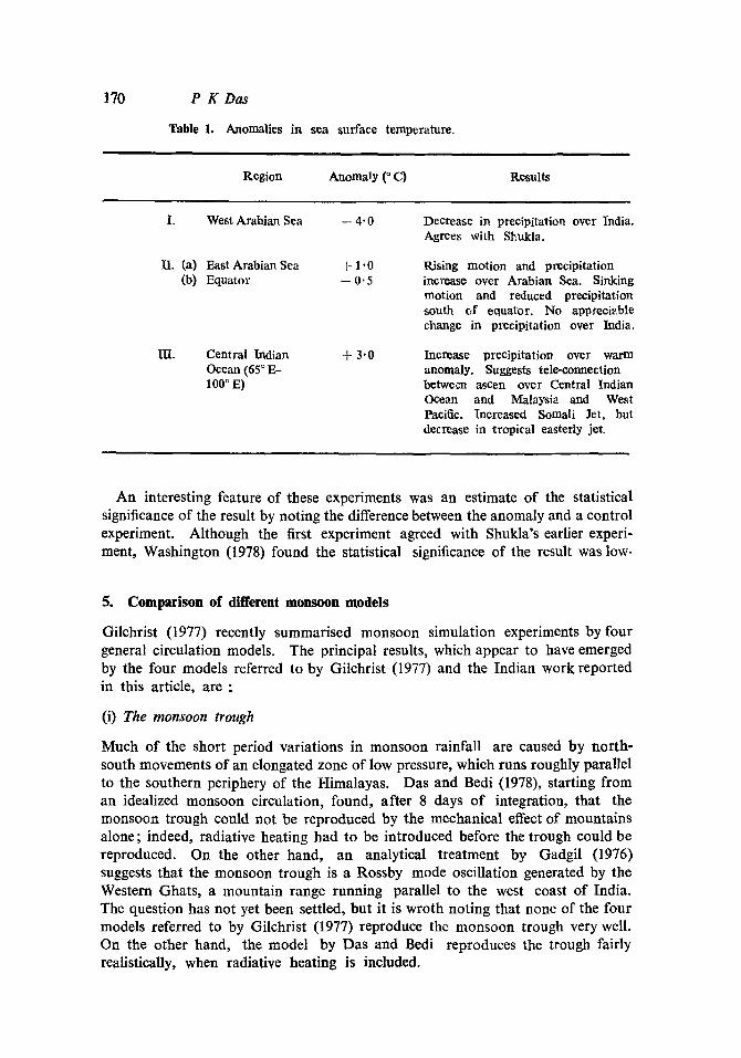
In a series of three experiments with the NCAR GCM model, Washington et al (1977) and Washington (1978) extended the earlier work of Shukla. The experi- ments in terms of anomalies in sea surface tempreature are indicated in table 1.

170 P K Das

Table 1. Anomalies in sea surface temperature.

Region Artomaly (~ C) Results

I. West Arabian Sea - 4 . 0 Decrease in precipitation over India. Agrees with Shukla.

II. (a) East Arabian Sea + 1"0 (b) Equator -- 0.5

Rising motion and precipitation increase over Arabian Sea. Sinking motion and reduced precipitation south of equator. No appreciable cha~ge in precipitation over India.

III. Central Indian + 3.0 Increase precipitation over warm Ocean (65 ~ E- anomaly. Suggests tele-eonnection 100~ between ascen over Central Indian

Ocean and Malaysia and West Pacific. Increased Somali Jet, but decrease in tropical easterly jet.

An interesting feature of these experiments was an estimate of the statistical significance of the result by noting the difference between the anomaly and a control experiment. Although the first experiment agreed with Shukla's earlier experi- ment, Washington (1978) found the statistical significance of the result was low.

5. Comparison of different monsoon models

Gilchrist (1977) recently summarised monsoon simulation experiments by four general circulation models. The principal results, which appear to have emerged by the four models referred to by Gilchrist (1977) and the Indian work reported in this article, are :

(i) The monsoon trough

Much of the short period variations in monsoon rainfall are caused by north- south movements of an elongated zone of low pressure, which runs roughly parallel to the southern periphery of the Himalayas. Das and Bedi (1978), starting from an idealized monsoon circulation, found, after 8 days of integration, that the monsoon trough could not be reproduced by the mechanical effect of mountains alone; indeed, radiative heating had to be introduced before the trough could be reproduced. On the other hand, an analytical treatment by Gadgil (1976) suggests that the monsoon trough is a Rossby mode oscillation generated by the Western Ghats, a mountain range running parallel to the west coast of India. The question has not yet been settled, but it is wroth noting that none of the four models referred to by Gilchrist (1977) reproduce the monsoon trough very well. On the other hand, the model by Das and Bedi reproduces the trough fairly realistically, when radiative heating is included.

Numerical simulation of the Indian monsoon

(ii) Mountain effects

171

The best known experiment is due to Hahn and Manabe (1975). The model was partially successful in reproducing the westerly jet, but it overestimated the tropical cyclone activity in the western Pacific, and underestimated the monsoon intensity in the north Bay of Bengal. The model was successful in simulating an anticyclonic circulation at 200 mb over Tibet. Another interesting result was that without mountains the monsoon was extremely weak. Hahn and Manabe found, for example, that without the mountains the monsoon never moved north of about 15 ~ N. It is worth noting that the inclusion of mountains in this model was not sufficient by itself to generate the monsoon trough--a result which was also suggested by Das and Bedi.

(iii) Rainfall

Observations by satellites have been compiled by Rao et al (1976). They now provide us with better estimates of rainfall over the oceanic regions. The Meteoro- logical Office model by the U.K. meteorological service simulates, in some measure, the heavy rainfall over the western parts and over the eastern Himalayas, but the Himalayan maximum is located much farther north than its observed loca- tion. In general, model simulation of rainfall has not been very satisfactory so far. This could be par tly attributed to lack of data on cloud ensembles over the Indian Ocean and the Arabian Sea. It is expected that data collected during the Monsoon Experiment (MONEX)in 1979 will partly remove this limitation.

(iv) Monsoon depressions

These depressions form over the north Bay of Bengal and gradually move north- westwards along the axis of the monsoon trough. None of the four global models in Gilchrist's review appear to simulate the formation of these depressions very well. During 1977, a stationary polygon of four ships from the USSR was aligned over the north Bay of Bengal to study monsoon effects. They were able to capture one monsoon depression. Das and Bedi observed that, with their model, if the mountains were removed, the predicted track of this depression would have been far more to the north than what was actually observed. But, when the Himalayas were included in the model, the predicted track was more towards the west, in agreement with the observed track. Modelling experiments appear to provide a useful technique for study of the formation and movement of monsoon depressions.

(v) Anticyclonic circulation

At 200 mb most monsoon models have succeeded in being able to reproduce the observed anticyclone over Tibet and, in general, over India during the monsoon. Hahn and Manabe were also able to simulate, partially a reverse Hadlay cell, postulated by Koteswaram (1963) on account of the latent heat released by heavy rainfall on the southern slopes of the Himalayas.

172 P K Das

(vi) lnterhemispherical interaction

Monsoon models need to simulate interhemispherical interaction because the genesis of the monsoon is in the southern hemisphere. Interaction on the shorter time scales is not yet well understood because of sparse data over the equatorial regions. Charney (1969) pointed out that the equatorial regions would tend to trap the northward passage of a wave, because these regions were characterized by zonal winds which moved westwards relative to the phase speed of the wave. The suggestion has been made that both the northern and southern hemispheres could be considered independent of each other for transient waves, that is, on time scales smaller than seasonal. But, Webster and Curtin (1975) and Mura- kami and Unni Nayar (1977) suggest, from observational data, that there are areas where kinetic energy appears to flow from the southern to the northern hemisphere. Webster etal (1978) suggest that there are periods, when weak easterlies or westerlies prevail over the equator, that permit the northward move- ment of transient wave disturbances. A detailed investigation of this problem with data collected during the recently concluded Monsoon Experiment (MONEX) would be interesting, because the phenomenon is similar to the trapping of waves propagating vertically from the troposphere to the stratosphere (Matsuno 1970).

6. Results of modelling experiments in India

We shall conclude this survey with a few results, which have been obtained with the model described in w 2.

- - A .

I 2 0 , 6 0 , 1 0 0 , 1 4 0 E ~

' , \

I \~..~ ~-- 320 , ~--~_~ \ ,

I ~o 60 1(3o .~OE

Surfoce

20 301 '

20 60 100 140E

10 raps

Arrows indicate wind Figure 1. Initial stato with moridional and vextical shoar. directions and figures roprese~t t�9

Numerical simulation of the Indian monsoon 173

Figure 1 depicts an idealised initial state. It has westerlies at the surface but, at 500 rob, the westerlies weaken south of 30 ~ N. At 300 mb the tropospheric westerlies are replaced by easterlies to the south of 30 ~ N. This corresponds, approximately, to the monsoon circulation which has a trasition at 500 mb between lower westerlies and upper easterlies. The easterlies aloft are generated by an anticyclonic circulation over the monsoon regime. The vertical and meri- dional wind shears in figure 1 were carefully adjusted so that the initial state was not dynamically unstable. It may be noted, however, that there was an anticyclonic wind shear in the initial state along 30 ~ N.

Figure 2 indicates the result of integrating the model up to 8 days with moun- tain forcing. The dotted area indicates the idealised Himalayas which were introduced into the model. The figure shows that no monsoon trough was gene- rated as the result of forcing by mountains. The Western Ghats and the Burmese mountains were also included in the model, although they have not been explicitly shown in the figure. It was interesting to observe the anticyclonic curvature of isobars as the wind traversed the Western Ghats. The deep lee trough to the east of the Himalayas was another important feature.

In figure 3 the result of 8 days integration is shown with the additional inclusion of radiative forcing. It was interesting to note in this figure that the model was able to reproduce the monsoon trough. This suggests that the formation of the monsoon trough is not merely a mechanical effect caused by the alignment of mountains. Radiative imbalances play an important part in its formation. The model, however, generates a well-marked anticyclone over Iraq and Iran. This was unrealistic. The reasons for this are now being investigated. In figure 4 we again illustrate 8 days integration, but with the addition of a heavy dust load over north-west India. We see that the model succeed in giving a more realistic picture of the monsoon trough, but the unrealistic anticyclone over the middle east still remains in a weakened form.

40 60 80 100 120~ 6 0 " N I l l l I I ' l I 1 1 6 0 oN

I L --4 t - - , ~ 9 8 8 ~ ---..---988

40 ~ 40

lOOO 20 2 0

0 0 40 " 60 8 0 1 0 0 t20~

Figure 2. Sea level chart after 8 days with only mountains.

174 P K D a s

60~

40

20

0

40 60 80 100 120"E I i I t I r I i 1 6 0 " N

, v ~ , . 1 / f ~ - ~ " ', ~-Iooo i, ( 99~ - looo 000~ 994

40 60 80 100 J200

Figure 3. Same as figure 2, but with mountains and radiative effects.

60~ f

4(3

20

40 60 80 100 120"E

1 I I I I I I 1 I

- ~ ~ / ~ ~ ~ . . . . . _ _ ~ , ,

I J I I l I I ~ I t 40 60 BO I(90 120~

60eN

40

20

Figure 4. Same as figure 2, with additional cooling over north-west India due to dust.

During the Indo-Soviet expedition of 1977 the four USSR ships, aligned in the form of polygon, were able to provide useful data on a monsoon depression in the Bay of Bengal on 20 August 1977. We used the model to predict the movement of this depression with and without mountains. The track without mountains was very far to the north west. This is shown by a full line in figure 5. On the other hand, when mountains were included (dotted line with triangle) the computed track was in fairly good agreement with the observed path of depression (dotted line with circles). While these experiments are in a prelimi-

Numerical simulation of the Indian monsoon 175

30N i I I I I r"

Seo level posit~on

25- ~+~ , ~ " 22

5 N , 70E BO 9 0 IOOE

Figure 5. Observed and predicted d~aression tracks. Full line indicates predicted track without mountains, dotted line with triangles indicates predicted track with mountains. Dotted line with circles indicates the observed track.

nary stage, they illustrate the fact that many of the well-known features of monsoon could be reproduced with the help of simple three-dimensional primi- tive equation models.

7. Summary and conclusions

We have presented in this review, a broad picture of the work that is currently in progress in India. There are certain important facets of modelling which we have not touched, because the work in this area is still in a preliminary stage. As examples, we quote spectral models or ocean-atmosphere coupled models, on which much work remains to be done. But it is encouraging to note that it is possible to simulate a number of interesting features of the Indian monsoon by simple models. It seems reasonable to expect better results in future by extending the capability of these models. We have, for example, partly succeeded in simulating the monsoon trough, but the models have not yet been able to throw much light on why the trough moves periodically north and south of its normal location. A similar situation prevails on the question of the formation of monsoon depressions. The models so far have not been able to simulate the formation of a depression starting from an initial stage, but there has been some success in predicting the course of a depression after it has formed. There are other areas where further modelling work is needed; the formation of the Intertropical Conver- gence Zone (ITCZ) is an example of such a field. It is not yet clear whether the ITCZ merely loses its identity with the advance of the monsoon, and a secondary low pressure area forms over India, or whether the ITCZ gradually moves north- wards across Arabia. Simple barotropic models, using shallow water equations by Webster (1977), suggest wave-wave interactions near the equator could provide a zonal flow, which resembles the ITCZ.

176 P K Das

In addition to the study of basic synoptic features, there are also interesting physical systems which the models have not yet considered. The role of aerosols and dust particles is an example. How does the heavy dust-load over north-west India, just before the onset of the monsoon, change the heat balance of the atmos- phere ? It should be possible to determine whether the role of dust is primarily to scatter or to absorb radiation, by numerical models.

There exists a wide variety of problems where modelling technique could be usefully employed. A major thrust is needed in (a) collecting data on different physical processes, (b) on monitoring changes in certain parameters of the monsoon and (c) on developing suitable techniques for improving the performance of models.

8. Acknowledgement

The author is happy to contribute this article for the Seventieth birthday of Professor P R Pisharoty. He has been a source of encouragement for research on the Indian monsoon. His work in 1955 on the flux of kinetic energy from different latitude belts, which later won him international recognition, did much to generate interest in modelling experiments in India.

References

Abbott D A 1978 in Monsoon dynamics ed. T N Krishnamurti, Birkhauser (reprinted from Pure and Applied Geophys.) 115 1111-1130

Arakawa A 1966 Y. Comp. Phys. 1 119 Arakawa A and Schubert W H 1974 Y. Atmos. Sei. 31 674 Baer F 1977 Beitr. Phys. Atmos. 50 350 Cadet D and Olory Togbr P 1978 Q.J.R. MeteoroL Soe. 104 442, 971-977 Charney J G 1969 J. Atmos. Set. 26 182 Corby G A, Gilchrist A and Rowntree P A 1977 Methods in Comp. Phys. 17 67-110 Das P K, Sinha M C and Balasubramanyam V 1974 Q. ZR. MeteoroL Soc. 100 437 Das P K and Bedi H S 1977 Indian J. Meteorol. Hyd. Geophys. 29 1 375 Das P K and Bedi H S 1978 Proe. IUTAM]IUGG Symposium on Monsoon Dynamics, IIT, Delhi

(in press) Eggor J 1972 Tellus 24 324-544 Egger J 1974 Men. Weather Rev. 102 847 Gadgil S 1976 Prec. Syrup. on Tropical Monsoons, Puno p. 59 Gilchrist A 1977 The simulation of the Asian summer monsoon by general circulation models,

Pageoph, Basel 115 1431 Godbole R V, Kelkar R R and Murakami T 1970 Indian J. Meteorol. Geophys. 21 43 Gordon A H and Taylor R C 1975 IIOE Meteorol. Monograph, University of Hawaii 7 112 Hahn D G and Manabe S 1975 J. Atmos. Sei. 32 1515 Jones R W 1977 J. Atmos. Sei. 34 1528 Kasahara A 1974 Men. Weather Rev. 102 509 Kasahara A 1977 Methods in Comp. Phys. 17 1 Kondo H and Nitta T 1979 J. Meteorol. See. Jpn. 57 300 Koteswaram P 1963 Aust. Meteorol. Mag. 42 35 Kraus E B 1977 Modelling and prediction of the upper layers of the ocean (New York: Perga-

mon Press) 1 325 Krishnamurti T N, Kanamitsu M, Coselski B and Mathur M B 1973 Tellus 6 523 Leith C E 1979 Nonlinear normal model inltialisation and quasi-goostrophic theory, unpublished

top NCAR Ms. 0901-'/9-01 p. 42

Numerical simulation of the Indian monsoon 177

Machonhauer B 1976 Ann. MeteoroL (Nene Folge) I I 135 Manabe S, Hahn D G and Holloway J L 1974 J. Atmos. Sci. 31 43 Marchuk G I 1974 Numerical methods in weather prediction (New York: Academic Press) p. 277 Martin H C and Carey G F 1973 Introduction tofinite elements (New York: McGraw Hill)p. 386 Matsuno T 1966 J. Meteorol. Soc. Jpn. 44 85 Matsuno T 1970 J. Atmos. Sci. 27 871 Mollor G L and Yamada 1974 J. Atmos. Sci. 31 1791 Mintz Y, Katayama A and Arakawa A 1972 Numerical simulation of the seasonally and inter-

annually varying tropospheric circulation Prec. Survey Conf. Climatic Impact Assessment Program, Department of Transportation, Washington D.C., pP. 194-216

Miyakoda K and Rosati A 1977 Men. Weather Rev. 105 1092 Murakami T and Unni Nayar M S 1977 Atmospheric circulation during December 1970 through

February 1971, Men. Weather Rev. 105 1024 Nakamura H 1978 Y. MeteoroL Soc. Jpn. 56 317 Phillips N A 1957 J. Atmos. Sci. 14 184 Phillips N A 1959 Men. Weather Rev. 87 333 Pisharoty P R 1955 The kinetic energy of the atmosphere, Fin. Rep. Gen. Circulation Project, No,

AF[9/122-48, P. 155 Pisharoty P R 1965 Prec. Symp. on Meteorol. Results of IlOE, India Met. Dept., Bombay p. 120 Ramanathan Y 1978 Determination of cloud clustcr properties from Monsoon-77 data

Prec. 1UTAM/IUGG Symp. on Monsoon Dynamics, IIT, N. Delhi (Cambridge Univ. Press-- under publication)

Rao G V, Bolhofor and Boogard H Van De Indian J. Meteorol. Hyd. Geophys. 29 303-307 Rao M S V, Abbott and Theon J S 1976 Satellite derived global oceanic rainfall atlas (1973 and

1974) NASA SP-410, NASA, Washington Richtmeyer R D and Morton K W 1967 Difference methods for initial value problems (New York ;

Wiley Interscience) Sadourny R 1977 Structure of real and model flows, Workshop on Numerical Weather Prediction,

unpubl shed lecture notes, IIT, Delhi p. 45 Sakor N J 1975 A ll-layer general circulation model, Tech. Note II/37, U.K. Met. Cff, ce, UK. Shaw D B 1978 Indian J. Meteorol. Hyd. Geophys. 29 361 Shukla J 1975 J. Atmos. Sci. 32 503 Shukla J and Bangaru B 1978 Prec, JOC Study Conference on Climate Models (USA : Washington

DC) Singh S S and Saha K R 1976 Proc.Symp. on tropical Monsoons, Puno pp. 43-50 Sinha M C and Sharma O P 1978 Vertical velocity in monsoon circulation:Prec. IUTAM/IUGG

Syrup. on Monsoon Dynamics, Camb. Univ. Press (in press) Sommeria G 1976 J. Atmos. Sci. 33 216 Starr V P 1945 J. Meteorol. 2 227 Stone P H, Chow S and Quirk W J 1977 Men. Weather Rev. 105 170 Sundquist H 1978 On incorporation of orography into numerical prediction medals, Proc; IUTAM/

IUGG Symp. on Monsoon Dynamics, IIT, New Delhi, Camb. Univ. Press (in press) Varma S 1978 A one-dimensional model of the planetary boundary layer for monsoon studies;

Prec. IUTAM/IUGG Symp. on Monsoon Dynamics, Camb. Univ. Press (in press) Washington W M and Daggupaty S M 1975 Men. Weather Rev. 103 105 Washington W M 1978 A review of general circulation model experiment on the Indian monsoon;

Prec. IUTAM/IUGG Symp. on Monsoon Dynamics, IIT, New Delhi, Camb. Univ. Press (in press)

Washington W M, Chervin R M and Rao G V 1977 Pure Appl Geophys. 115 1335 Webster P J 1978 Indian J. MeteoroL Hyd. Geophys. 29 235 Webster P J and Kurtin D G 1975 Y. Atmos. Sci. 32 t848 Webster P J, Chou L and Lau K M 1978 Mechanism offocting the state, evolution and transition

of the planetary scale monsoon; Monsoon dynamics ed. T. N Krishnamurti, Birkhauser (reprinted from Pure and Applied Geophysics 115 1463-1492)

v. (AY--~