Numerical Simulation of Supersonic Jet Flows and

their Noise

S.-C. Lo∗, G. A. Blaisdell†, and A. S. Lyrintzis‡

School of Aeronautics and Astronautics

Purdue University

West Lafayette, IN 47907

Large-eddy simulations (LES) of a circular supersonic fully expanded jet and an under-expanded jet are performed. Both jets operate at a design Mach number 1.95, and thecorresponding fully expanded Mach number for the underexpanded jet is 2.20. Since thesimulations do not include the nozzle geometry explicitly, the effects of the inflow condi-tions (such as the forcing modes and shear layer thickness) on the near field statistics andfar field noise are investigated. The near field data are collected from the LES and thenthe far field noise is computed by the Ffowcs Williams-Hawkings (FWH) surface integralmethod. The results show that removing the lower forcing modes increases the centerlinevelocity decay rate, the peak turbulence intensities, and the overall sound pressure level.However, reducing the inflow shear layer thickness has the opposite effect and achievesa better agreement with the experiments in both near field statistics and farfield noise.Similar trends hold for the underexpanded jet in near field statistics; however, the numberof shock cells is underpredicted and is insensitive to the inflow conditions. This may bedue to contamination by spurious numerical fluctuations caused by the shocks. Furthersimulations including shock capturing schemes are needed.

I. Introduction

The noise radiated by jet engines has received more attention recently. Due to the strict regulations onaircraft with high jet noise emission near airports, most jet engine designers are trying to reduce the noiselevels in newly designed jet engines. In order to achieve this objective, expanding the bounds of knowledgein jet aeroacoustics has become necessary. With the progress of commercial aircraft design, some of therecently developed commercial aircraft (such as the Boeing 777 and 787) are equipped with high by-passratio engines which can operate at supercritical pressure ratios. In addition to turbulent mixing noise, whichis generated by instabilities of the shear layer near the jet lip, shock associated noise can be generatedwhen a supersonic jet engine operates at an off-design condition. This (broadband) shock associated noiseis generated by the interactions between the turbulence and the shock cells which occur downstream of thenozzle exit. Therefore, accurate prediction of supersonic jet noise has become an important step in the designof new low noise emission engines.

Traditional jet noise studies rely heavily on experiments. With the advances of fast supercomputers,the application of direct numerical simulation (DNS) to jet noise prediction is becoming possible. DNSsolves for the dynamics of all the relevant length scales of turbulence and does not use any turbulencemodels. However, due to the wide range of time and length scales in high Reynolds number turbulentflows, the application of DNS to industrially relevant jets is still infeasible. Large eddy simulation (LES),which computes the large scales directly and models the effect of the small (subgrid) scales, yields a cheaperalternative. As a result, LES can be used as a tool for jet noise prediction since it is capable of simulatinghigh Reynolds number flows at a fraction of the cost of DNS. The far field noise then can be estimatedusing near field variables directly computed by LES by coupling with acoustic methods (such as the Ffowcs

∗Graduate Teaching Assistant, Student Member AIAA.†Associate Professor, Senior Member AIAA.‡Professor, Associate Fellow AIAA.

1 of 18

American Institute of Aeronautics and Astronautics Paper 2008-2970

14th AIAA/CEAS Aeroacoustics Conference (29th AIAA Aeroacoustics Conference)5 - 7 May 2008, Vancouver, British Columbia Canada

AIAA 2008-2970

Copyright © 2008 by S.-C. Lo, G. A. Blaisdell, and A. S. Lyrintzis. Published by the American Institute of Aeronautics and Astronautics, Inc., with permission.

Williams-Hawkings method1 or Lighthill’s acoustic analogy2). The basic idea is briefly described as follows.The near field variables computed by the LES are stored on a certain control surface or within a volumeevery few time steps. After collecting enough data, the far field pressure fluctuation can be computed byperforming either a surface or volume integral of those stored variables.

The LES approach has been used in supersonic jet simulations by several researchers. The first uses ofLES as an investigation tool for jet noise prediction was carried out by Mankbadi, et al.3 They performedan axisymmetric LES computation of a fully expanded Mach 1.5 and Reynolds number 1.27 × 106 jet andapplied Lighthill’s theory to calculate the far field noise; however, no quantitative comparisons with theexperimental results are made. Freund et al.4 used DNS with 22 million grid points to simulate a lowReynolds number 2000 supersonic fully expanded jet. Both the near field statistics and the sound pressurelevels are presented. Although no comparison of the near field statistics with any experimental results isshown, the sound pressure levels match well with the experimental data at similar flow conditions. DeBonisand Scott5 used LES with the Smargorinsky subgrid scale (SGS) model to study a cold Mach 1.4 fullyexpanded jet with a Reynolds number of 1.2 million. Their simulation accurately captures the physics ofthe turbulent flow and the time averaged velocity fields agree with experimental data. Al-Qadi and Scott6

used a sixth-order compact scheme and a TVD type characteristic filter developed by Yee et al.7 to studya 3-D underexpanded rectangular jet. The results demonstrate that the schemes they used are capable ofresolving the unsteady complex near field features. Bodony et al.8 used LES to simulate and comparea fully expanded jet and an underexpanded jet without using any shock capturing schemes. They foundMach waves contribute significantly to the near field pressure of the underexpanded jet. Berland et al.9

used LES to investigate the screech tones generated by a 3-D plane underexpanded jet. Their computationreproduces the screech tone generation phenomenon, and shows the feasibility of the direct computation ofnoise involving such a feedback loop with high-order algorithms. Viswanathan et al.10 study the flow andthe noise characteristics on both heated and unheated jets for round and beveled nozzles. To avoid therequirement of the massive computational resources needed by the LES approach for the near wall regionof the boundary layer, a two-step RANS/LES methodology11 is adopted, which uses a RANS calculation toprovide a nozzle boundary layer then LES is performed in a second step for the external plume on a coarsegrid. Their simulations cover a wide range of jet velocities, i.e. from Mach 0.4 to Mach 1.9, and the predictednoise levels are comparable with the experimental results, within about 2 to 3 dB. In addition, Mach waveradiation is clearly observed from the contours of pressure-time derivative, indicating the source of noise.Li and Gao12 use an unsteady Reynolds averaged approach with the dispersion-relation-preserving (DRP)scheme to investigate the near-field screech of Mach 1.17 to 1.60 underexpanded jets. To capture the shocksthe variable stencil Reynolds number method is utilized. The shock cell structures and the radial densityprofile compare well with the experiment. In addition, the difference between the near field sound pressurelevels of their simulations and the experiments are within 4 dB.

Our 3-D LES methodology has demonstrated its success in the prediction of subsonic jet noise.13–17

However, the ability of our method to predict supersonic jet flows and the related noise fields has notbeen validated. Therefore, the objective of the current study is to investigate the capability of our 3-DLES methodology for supersonic jet simulations. The following sections briefly describe the LES numericalmethod, surface integral acoustic method, case and grid information, and results of our near-field statisticsand far-field noise.

II. Numerical Methods

A. 3-D LES methodology

We briefly describe the LES methodology that we used in this study. The 3-D LES code was originallydeveloped by Uzun.13 The code is designed for the study of subsonic turbulent jet noise at high Reynoldsnumbers. It is an unsteady, Favre-filtered, compressible Navier-Stokes solver. The sixth-order compactmethod developed by Lele18 is used for spatial discretization on the internal points. For the points on theboundary, however, a third-order one-side compact scheme is used, and the points next to the boundariesare computed by a fourth-order compact scheme. The time advancement scheme is the classical forth-orderRunge-Kutta method. In order to prevent spurious reflections, Tam and Dong’s radiation and outflowboundary conditions19,20 are implemented on the boundaries. In addition, a sponge zone is attached atthe outflow boundary to prevent unwanted reflections caused by strong vortices passing through the outflowboundary. It is known that the compact scheme can produce high-frequency spurious modes which arise fromthe boundary conditions, unresolved scales, and mesh non-uniformities, and cause numerical instabilities.

2 of 18

American Institute of Aeronautics and Astronautics Paper 2008-2970

In order to eliminate these spurious modes and keep the scheme stable, a sixth-order tri-diagonal implicitspatial filter proposed by Gaitonde and Visbal21 is used in this study. We apply this spatial filter once aftereach full Runge-Kutta time step, and the filter coefficient, αf , is set to 0.47.

This LES solver can use an eddy-viscosity subgrid scale (SGS) model (such as the classical or a localizeddynamic Smagorinsky (DSM) model) to dissipate the turbulent energy. Although the DSM model canalleviate the need to specify the Smagorinsky constant for a given problem, using it usually requires about40% more computational time than the only using spatial filter. A spatial filter can also emulate the effectsof a subgrid scale model, acting as an implicit SGS model. A discussion of the two methods can be found inreference.22 For the current study both DSM and a spatial filter are used as SGS models.

Since the current simulations do not include an explicit nozzle, some special treatments on the inflowboundary must be specified. A hyperbolic tangent velocity profile used by Freund23 is specified on the inflowboundary as

u(r)Uj

=12

{1− tanh

[r0

4θ0

(r

r0− r0

r

)]}(1)

where r =√

y2 + z2, r0 = 1, Uj is the jet centerline velocity, and θ0 is the inflow momentum thickness.Here, θ0 is used to control the thickness of the inflow shear layer. A higher value of θ0 implies a thicker shearlayer. In order to investigate the influence of the initial shear layer thickness, two values of θ0 (0.09r0 and0.06r0) are used in this study. The former value has been used by Bodony and Lele24 and Lew et al.16 andthey were able to achieve good agreement with the experiments on turbulent statistics and farfield noise.For laboratory jets, however, the measured value of θ0 is usually an order of magnitude or more smaller(∼ 2 × 10−2r0)25 compared to that used in LES and DNS of jets. For the inflow density profile, we alsoadopt the formula from Freund,23

ρ(r)ρj

= (1− ρ∞ρj

)u(r)Uj

+ρ∞ρj

(2)

For the underexpanded jet, a hyperbolic tangent profile similar to equation (1) is used to specify the inflowpressure profile.

In the actual jet flow, the nozzle lip can reflect and scatter acoustic waves into jet’s initial shear layerand excite the mean flow. Since the current simulations do not include the nozzle, in order to mimic itsfunction and promote natural transition from an initially quasi-laminar annular shear layer, the vortex ringforcing approach proposed by Bogey and Bailly26 is used in this study. This is done by putting a vortexring at approximately one jet radius downstream of the inflow boundary to generate randomized velocitypertubations. The streamwise (v′x) and radial (v′r) velocity perturbations are then added to the local velocitycomponents. However, velocity perturbations in the azimuthal direction are not added. The expressions forv′x and v′r are

v′x = αUxringU0

nmodes∑n=0

εn cos(nΘ + ϕn) (3)

v′r = αUrringU0

nmodes∑n=0

εn cos(nΘ + ϕn) (4)

where Θ = tan−1(y/z), εn and ϕn are randomly generated numbers that satisfy −1 < εn < 1 and 0 < ϕn <2π. U0 is the mean jet centerline velocity at the inflow boundary, and the total number of forcing modes,nmodes + 1, is 16. The parameter that determines the amplitude of the forcing is α and it is set to 0.007 inthis study. The mean axial (Uxring ) and radial (Urring ) velocity components of the vortex ring are given as

Uxring = 2r0

r

r − r0

∆0exp

[− ln (2)

(∆(x, r)

∆0

)2]

(5)

Urring = −2r0

r

x− x0

∆0exp

[− ln (2)

(∆(x, r)

∆0

)2]

(6)

where r =√

y2 + z2 6= 0, ∆0 is the minimum grid spacing in the shear layer, and ∆(x, r)2 = (x − x0)2 +(r − r0)2. The center of the vortex is located at x0 which is r0 in our case. Studies regarding the effect ofthis inflow forcing on subsonic jets can be found by Lew et al.27 and Bogey and Bailly.28

Because both the compact scheme and the spatial filter require all the data points along a given gridline to solve the linear system, a transposition strategy13 is used for the parallelization. Initially, the grid

3 of 18

American Institute of Aeronautics and Astronautics Paper 2008-2970

is partitioned along the z direction, and the derivatives and the filtering are computed in both x and ydirections. Then the data are transposed for the computation in the z direction. Once the computationalong the z direction is finished, the data is transposed back to the initial configuration.

B. Surface integral acoustic method

The Ffowcs Williams-Hawkings (FWH) surface integral acoustic method1,29 is used to study far-field noiseof supersonic fully expanded jets. Due to the lack of experimental data, no noise calculations were made forthe current underexpanded jet cases. For a stationary permeable control surface, the disturbance pressureat an observer coordinate, ~x, and time, t, is composed of the thickness noise, loading noise, and quadrupolenoise. The quadrupole noise is neglected in this methodology.13 For details regarding the formulations ofeach pressure term and numerical implementation of the FWH method, the reader is referred to Uzun.13

III. Test Cases and Grid Information

A. Test cases

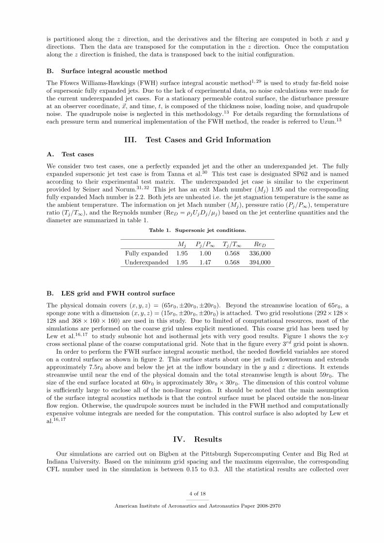
We consider two test cases, one a perfectly expanded jet and the other an underexpanded jet. The fullyexpanded supersonic jet test case is from Tanna et al.30 This test case is designated SP62 and is namedaccording to their experimental test matrix. The underexpanded jet case is similar to the experimentprovided by Seiner and Norum.31,32 This jet has an exit Mach number (Mj) 1.95 and the correspondingfully expanded Mach number is 2.2. Both jets are unheated i.e. the jet stagnation temperature is the same asthe ambient temperature. The information on jet Mach number (Mj), pressure ratio (Pj/P∞), temperatureratio (Tj/T∞), and the Reynolds number (ReD = ρjUjDj/µj) based on the jet centerline quantities and thediameter are summarized in table 1.

Table 1. Supersonic jet conditions.

Mj Pj/P∞ Tj/T∞ ReD

Fully expanded 1.95 1.00 0.568 336,000Underexpanded 1.95 1.47 0.568 394,000

B. LES grid and FWH control surface

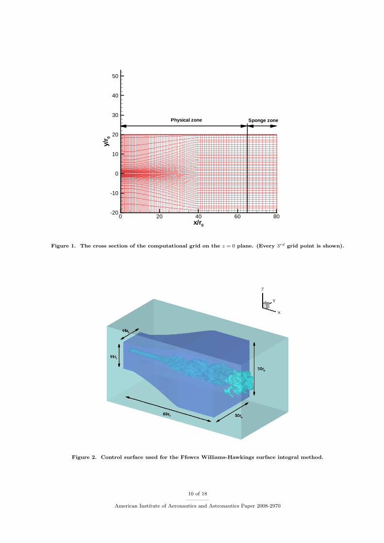
The physical domain covers (x, y, z) = (65r0,±20r0,±20r0). Beyond the streamwise location of 65r0, asponge zone with a dimension (x, y, z) = (15r0,±20r0,±20r0) is attached. Two grid resolutions (292×128×128 and 368 × 160 × 160) are used in this study. Due to limited of computational resources, most of thesimulations are performed on the coarse grid unless explicit mentioned. This coarse grid has been used byLew et al.16,17 to study subsonic hot and isothermal jets with very good results. Figure 1 shows the x-ycross sectional plane of the coarse computational grid. Note that in the figure every 3rd grid point is shown.

In order to perform the FWH surface integral acoustic method, the needed flowfield variables are storedon a control surface as shown in figure 2. This surface starts about one jet radii downstream and extendsapproximately 7.5r0 above and below the jet at the inflow boundary in the y and z directions. It extendsstreamwise until near the end of the physical domain and the total streamwise length is about 59r0. Thesize of the end surface located at 60r0 is approximately 30r0 × 30r0. The dimension of this control volumeis sufficiently large to enclose all of the non-linear region. It should be noted that the main assumptionof the surface integral acoustics methods is that the control surface must be placed outside the non-linearflow region. Otherwise, the quadrupole sources must be included in the FWH method and computationallyexpensive volume integrals are needed for the computation. This control surface is also adopted by Lew etal.16,17

IV. Results

Our simulations are carried out on Bigben at the Pittsburgh Supercomputing Center and Big Red atIndiana University. Based on the minimum grid spacing and the maximum eigenvalue, the correspondingCFL number used in the simulation is between 0.15 to 0.3. All the statistical results are collected over

4 of 18

American Institute of Aeronautics and Astronautics Paper 2008-2970

150,000 iterations to obtain converged statistics. The reason for so many steps to get converged statistics isbecause the Mach number drops to about 0.34 near the end of physical domain, which lowers the convergencerate. The averaged computational time required for a 4 million grid points case, including gathering nearfield statistics, is about 1 week by using 128 processors. The fine grid has about 9.4 million grid points andrequires 4 weeks computational time on 80 processors.

A. Fully expanded jet

1. Effect of Forcing Modes

First, we investigate the effect of which forcing modes are included on the supersonic fully expanded jet.The inflow momentum thickness, θ0, is set to 0.09r0, and the initial shear layer is resolved by about 13 gridpoints. The minimum grid spacing in the initial shear layer is 0.050r0. Designating rfx for each of thedifferent forcing strategies, we compare the results of four different cases (e.g. x = 0, 4, 6, 8). For example,rf0 means using all forcing modes, rf4 means removing the first four modes and using the remaining twelvemodes, and so on.

Figure 3 shows the variation of the mean streamwise velocity along the centerline for each of the forcingmode cases. The LES results by Bodony et al.8 are also added for comparison. All the LES results use 0.09r0

inflow momentum thickness and it is marked in the plot legend. The experimental results are from Lau etal.,33 Panda and Seasholtz,34 and Eggers.35 All the experimental jets are fully expanded and unheated.The temperature ratio (Tj/T∞) for Lau et al., Panda Mj = 1.4, Panda Mj = 1.8, and Eggers are 1.0, 0.73,0.61, and 0.5, respectively. Generally speaking, all the LES results decay faster than the Mach 1.8 and 2.22experimental jets. However, it is still difficult to compare the results with each other. As the plot shows,due to the differences in the jet Mach numbers, the potential core lengths are not the same for each of thecases. In order to understand the near-filed data and compare with other experimental results that havedifferent operating conditions, a rescaling of the x axis is necessary. Here, we adopt a procedure, called theWitze36 correlation, which is also used by Bodony and Lele.24 Through this rescaling, the differences in thecompressibility or Mach number which affect the length of the potential core can be accommodated. In theWitze correlation, the x axis is given by W = κ(x − xc)/r0, where κ = 0.08(1 − 0.16Mj)(ρ∞/ρj)0.22. Thepotential core length, xc/r0, is computed first, and then x/r0 is shifted axially. Then the data is rescaledusing the factor κ. Here, the length of potential core is defined by the location where the jet centerlinevelocity reduces to 95% of the inflow jet velocity.

Figure 4 shows the rescaled mean streamwise velocity along the centerline. It is clear that all the LESresults decay faster than the experiments. The rf0 forcing case decays more slowly than the other forcingcases. As we continue to remove the modes (from rf4 to rf8) the decay rate increases. It is noted thatour rf0 results are almost the same as Bodony’s results even though the methods are different. They usethe same compact method, but a cylindrical grid with (r × θ × x) = (128× 32× 256) and a different inflowforcing method. A quantitatively comparison of the centerline velocity decay rate in the far downstreamregion of the fully expanded jets is shown in figure 5. The velocity decay rate can be computed from theslope e.g. d(Uj/Uc(x))/d(x/2r0). The rf0 case has a predicted decay rate value of 0.124. However, bothPanda’s Mach 1.8 and Eggers Mach 2.22 jets have a decay rates of 0.080.

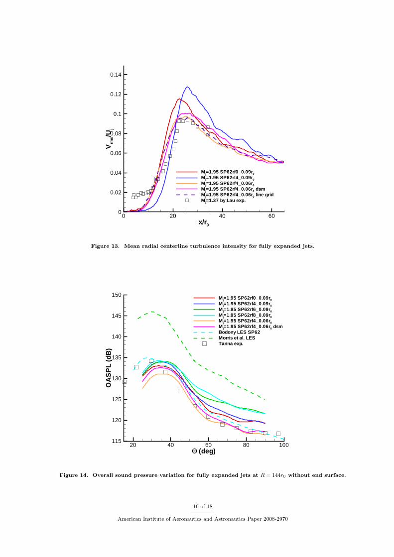
The axial and radial turbulence intensities (Urms and Vrms) along the axial centerline are shown in figures6 and 7. From the plot, an axial shift in the downstream direction and an increase of the peak intensity areobserved as the lower modes are removed. Comparing with figure 3, an earlier peak intensity correspondsto a shorter potential core. The potential core length increases if we continue removing the lower forcingmodes. The trends of our turbulent intensities is similar to the subsonic jet cases done by Lew et al.,27

but they have a roughly constant peak turbulence level. On the other hand, Bogey and Bailly37 observed areduction in the peak centerline turbulence levels when the lower modes are removed. Figure 8 shows therescaled axial centerline turbulence intensities. The trends of the LES jets are consistent with the experiment;however, we believe obtaining the same peak Urms value between the rf0 case and the experiment is just acoincidence. As reported by Lau et al.,33 the peak Urms and Vrms decrease with increasing jet exit Machnumber. Therefore, all of our LES results overpredict the peak intensity.

The effect of the inflow forcing modes can be summarized as follows. Removing the lower forcing modescauses an increase in both the jet centerline decay rate and the peak centerline turbulence level. In addition,it also shifts the location of the maximum Urms and Vrms downstream. However, the length of the potentialcore decreases as we remove the lower forcing modes. Our overprediction of the jet centerline decay ratemay possibly be attributed to two reasons: the inflow shear layer thickness and shocks which appear nearthe end of the potential core. The effect of shear layer thickness is described in the following section. The

5 of 18

American Institute of Aeronautics and Astronautics Paper 2008-2970

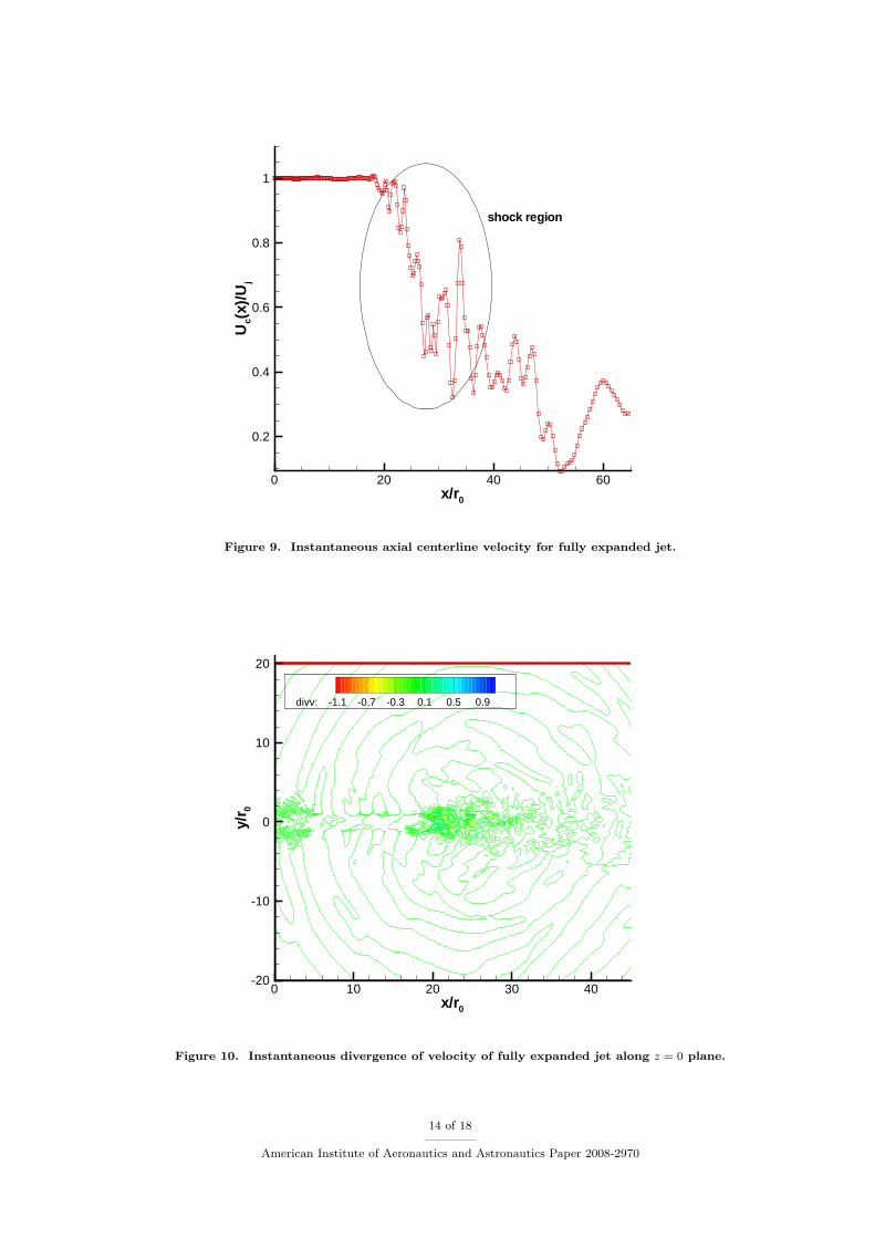
presence of shocks can be identified by looking at an instantaneous centerline streamwise velocity (figure9) or instantaneous contour plot of the divergence of velocity (figure 10). As shown in figure 9 for caserf8, large gradient regions (or shocks) appear in the circled region. Figure 10 shows the same case alonga constant z = 0 plane. The shocks appear in the regions where the divergence of velocity is large andnegative (e.g. at x ∼ 22r0). Since the current simulations do not use a shock capturing scheme, the spuriousnumerical oscillations caused by the shocks can propagate into flow field and contaminate the turbulencefluctuations. This may result in an increase of the peak turbulence level and centerline jet decay rate. Itshould be mentioned that the spatial filter used in this study is unable to damp out the numerical oscillationscaused by the shocks.

2. Effect of shear layer thickness

Results using 0.06r0 inflow momentum thickness are presented. About 13 grid points are used to resolvethe initial shear layer, and the minimum grid spacing in the initial shear layer is 0.035r0. Figure 11 showsthe scaled mean streamwise velocity along the centerline. The cases using the dynamic Smagorinsky (DSM)model, which increases the computational time by about 40%, is also shown in the figure. As report byBogey and Bailly,28 decreasing the initial shear layer thickness reduces the centerline velocity decay rate,and fluctuation levels. A similar phenomena can be observed in the figure. Both of the cases using 0.06r0

inflow momentum thickness have slower centerline velocity decay rates than the cases with thicker inflowmomentum thickness. However, adding the DSM model slightly increases the velocity decay rate comparedto the case without it. A fine grid case is added in the same figure to compare with the coarse grid cases.Due to the finer resolution, it has a slower centerline velocity decay rate than all the coarse grid cases.

Figures 12 and 13 compare the effects of a thinner shear layer on the mean axial and radial turbulenceintensities along the centerline. The cases using 0.06r0 inflow momentum thickness have lower peak tur-bulence intensity levels compared to the 0.09r0 cases. Adding the DSM model slightly increases the peakintensity values in both figures. This phenomenon corresponds to a faster centerline velocity decay rate,which is consistent with the results shown in figure 11. However, we still expect the peak Urms and Vrms tobe overpredicted, because of the higher centerline velocity decay rates.

3. Farfield noise

We gathered flow field data on the FWH control surfaces at every 5 time steps over a period of 50,000time steps during our LES run. The total acoustic sampling period corresponds to a time scale in whichan ambient sound travels about 5.8 times the streamwise domain length of the FWH control surface. Toperform the surface integral, this control surface is divided into 172 blocks for parallel computing and theaveraged computational time is about 12 hours using 172 processors on Bigben. Based on the grid resolutionaround the FWH control surface, and assuming 6 points per wavelength to accurately resolve an acousticwave, the maximum resolvable frequency corresponds to a Strouhal number 0.62. Here, the Strouhal numberis defined by Sr = fDj/Uj .

Figure 14 shows the overall sound pressure levels (OASPL) for the fully expanded jet case and theexperimental data,30 where the FWH prediction was computed without the end surface at 59r0. We computethe OASPL along an arc with a distance of R = 144r0 from the nozzle exit, and the observer angle, Θ, ismeasured relative to the jet centerline axis. This farfield distance and observer angle are used by Tanna etal.30 Other LES results are also put in the same figure for comparison. The OASPL result done by Bodonyand Lele24 is computed by Kirchhoff surface integral method, and the result by Morris et al.38 is computedby FHW method. In addition, the case by Morris et al. has the same temperature ratio and jet Machnumber as ours, but the Reynolds number (based on the jet diameter) is 100,000. It must be mentionedthat these LES results are taken from Bodony and Lele,39 which is scaled to a distance of 200r0. In orderto compare with current cases, same approach39 is used to scale to a distance of 144r0.

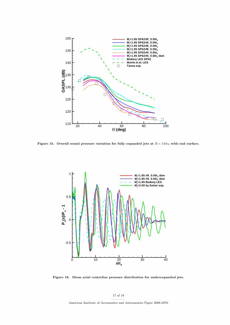
As we can see from the figure, Bodony’s case match very well with the experiment. Morris et al.overpredict the peak OASPL by about 10 dB. Removing the lower forcing mode increases the OASPL atall observer angles. This phenomenon is consistent with the increase of the peak turbulence intensity andthe report by Lew et al.27 All the 0.09r0 cases predict larger OASPL for Θ > 40◦. The peak value isshiftted about 5◦ higher compared to Tanna’s data. Cases rf4 to rf8 have about the same peak OASPLwith the experiment but case rf0 underpredicts the peak value by about 2 dB. Reducing the inflow shearlayer thickness (e.g. 0.06r0 cases) gives a better agreement with the experiment for Θ > 40◦. However, thepeak value is underpredicted about 4 dB and 2 dB for cases with and without the DSM model, respectively.Figure 15 shows the overall sound pressure levels (OASPL) for the fully expanded jet cases where the end

6 of 18

American Institute of Aeronautics and Astronautics Paper 2008-2970

surface at 59r0 has been included in the FWH computation. All the trends are similar to the cases withoutusing the end surface; however, the noise levels at small observer angles are slightly higher and match theexperiment a little better.

B. Underexpanded jet

Due to the shocks present in the potential core and downstream regions for underexpanded jets, numericalexperiments show that the compact scheme plus the spatial filter used for the fully expanded jet are unable tomaintain a stable computation. To overcome this problem, the DSM model is used to provide more numericaldissipation and keep the solver stable. Since the current simulations do not use any shock capturing schemes,this approach only works for cases with very weak pressure ratios, e.g. Pj/P∞ = 1.47. In addition, sinceour simulations do not include the actual nozzle in the computations, we found that the Tam and Dong’sradiation boundary19 does not work for underexpanded jets at inflow plane. This is because the potentialcore has a higher pressure than the ambient, and a solid wall may be needed to confine the flow to a specificregion. In order to solve this problem, we replace Tam and Dong’s radiation boundary conditions at theinflow plane with a characteristic boundary conditions by Whitfield and Janus,40 and we found this boundarycondition works well for current cases.

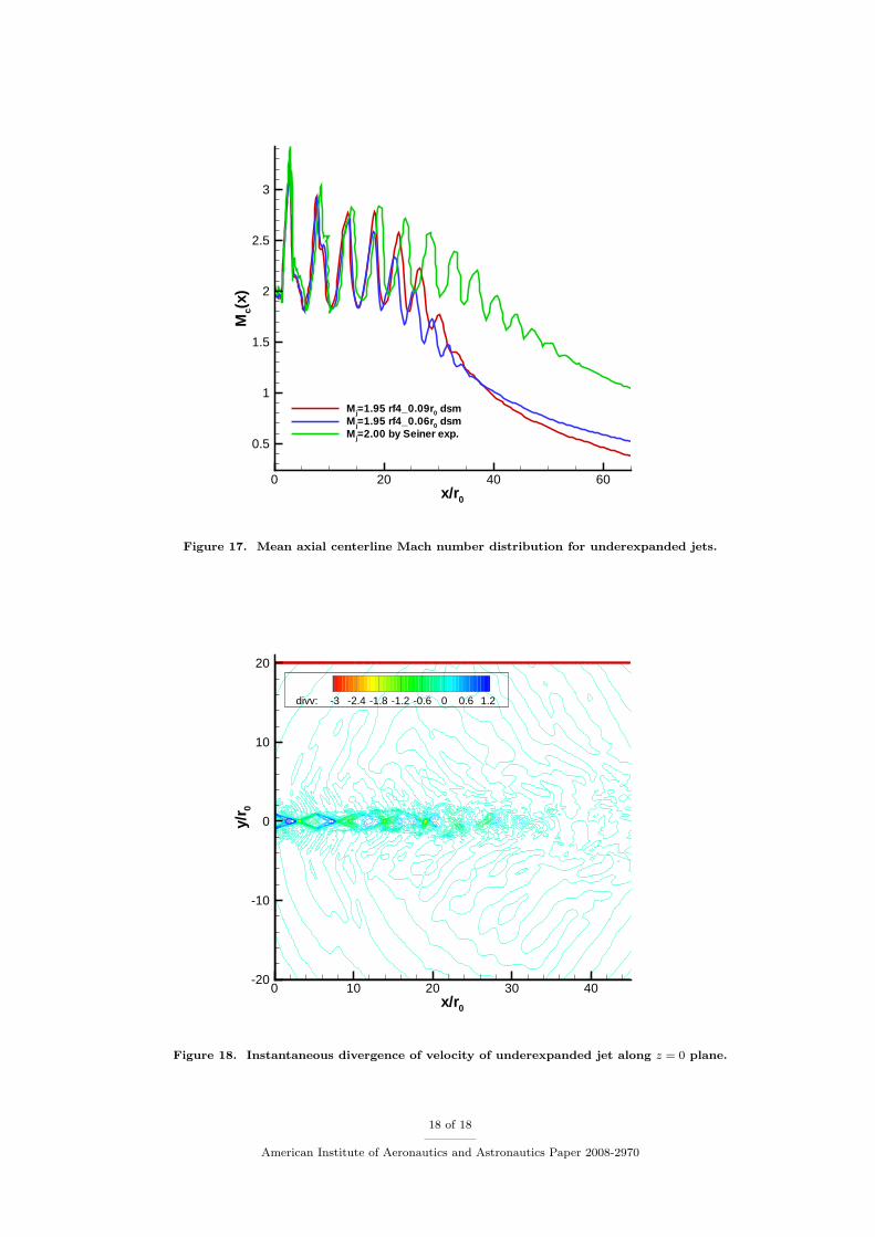
Figures 16 and 17 compare the variation of mean pressure and Mach number along the centerline. Theexperimental result is taken from Seiner and Norum,31 which has a design Mach number of 2.0 and a pressureratio (Pj/P∞) of 1.45. From figure 16, our LES results have about the same pressure oscillation amplitudeas the experiment when x 6 20r0, but this amplitude diminishes quickly for x > 20r0 and then completelydisappears at x ∼ 35r0. The reason that Bodony’s8 LES results predict smaller oscillation amplitudes maybe due to his grid (about 1 million points) being coarser than ours. Both cases with 0.09r0 and 0.06r0 inflowmomentum thickness predict about 9 visible shock cells. On the other hand, the experimental data hasabout 12 visible shock cells. The effect of the inflow momentum thickness on the number of the shock cellsseems insignificant. However, its effect becomes pronounced at x ∼ 35r0. As shown in figure 17 the 0.06r0

case has a slower Mach number decay which is closer to the experiment than the 0.09r0 case.The reason that all the LES results predict fewer shock cells than the experiment may be due to spurious

numerical oscillations caused by shocks appearing in the potential core. Figure 18 shows an instantaneouscontour plot of divergence of velocity for the case with 0.06r0 inflow momentum thickness. As shown in theplot, shocks appear in the regions where the divergence of velocity has a large negative value. Expansionwaves are shown as areas of positive divergence of velocity. The shock cells are revealed by alternatingregions of expansion and compression waves. In the downstream region eddy shocklets are apparent. Sinceall the LES simulations do not use shock capturing scheme, the spurious numerical oscillations generatedby the shocks can propagate into the flow field, and contaminate or magnify the physical oscillations. Thisphenomenon may be the reason that causes the potential core of our LES jet to break up earlier thanin the experiment. To verify this further simulations that include a shock capturing scheme, such as thecharacteristic filter approach,41 are needed.

V. Conclusion and Future Work

Large-eddy simulations of a circular supersonic fully expanded jet and an underexpanded jet are per-formed. The effect of variations of the inflow conditions (such as the forcing modes and the shear layerthickness) are investigated. The near field statistics show that removing the lower forcing modes increasesthe potential core length, centerline velocity decay rate, peak turbulence intensities, and far-field OASPL.However, reducing the inflow shear layer thickness has the opposite effect and achieves better agreementwith the experiments in both near field statistics and far-field noise. For the fully expanded jet we also ob-served that shocks may form at the end of potential core that generate spurious numerical oscillations thatcontaminate the physical fluctuations. Generally speaking, however, our subsonic 3-D LES methodology iscapable of simulating supersonic fully expanded jets without need of significant modifications. The effectsof inflow conditions that we investigated for the fully expanded jets are insignificant for the shock cell struc-ture of underexpanded jets. Due to these shock cell structures within the potential core, the contaminationfrom spurious numerical oscillations becomes more significant. Our underprediction of the number of shockcells may be caused by this problem. Further simulations including shock capturing schemes are needed toinvestigate this issue.

7 of 18

American Institute of Aeronautics and Astronautics Paper 2008-2970

VI. Acknowledgements

We would like to thank Dr. Ali Uzun from Florida State University who provided both his 3-D LES andFWH aeroacoustic codes. In addition, the S.-C. Lo would like to thank the High Performance Applications(HPA) group at Indiana University for providing assistance in setting up a useful computational environ-ment. Finally, S.-C. Lo gratefully acknowledges the support of the Purdue Research Foundation/ComputingResearch Institute (PRF/CRI) Special Incentive Research Grant (SIRG).

References

1Lyrintzis, A. S., “Surface integral methods in computational aeroacoustics - from the (CFD) near-field to the (acoustic)far-field,” International Journal of Aeroacoustics, Vol. 2, No. 2, 2003, pp. 95–128.

2Lighthill, M. J., “On the sound generated aerodynamically: I, general theory,” Proc. Royak Soc. London A, Vol. 211,1952, pp. 564–587.

3Mankbadi, R. R., Hayder, M. E., and Povinelli, L. A., “Structure of supersonic jet flow and its radiated sound,” AIAAJournal , Vol. 32, No. 5, May 1994, pp. 897–906.

4Freund, J. B., Lele, S. K., and Moin, P., “Direct numerical simulation of a Mach 1.92 turbulent jet and its sound field,”AIAA Journal , Vol. 38, No. 11, 2000, pp. 2023–2031.

5DeBonis, J. R. and Scott, J. N., “A large-eddy simulation of a turbulent compressible round jet,” AIAA Paper No.2001-2254, May 2001.

6Al-Qadi, I. M. A. and Scott, J. N., “High-order three-dimensional numerical simulation of a supersonic rectangular jet,”AIAA Paper No. 2003-3238, May 2003.

7Yee, H. C., Sandham, N. D., and Djomehri, M. J., “Low-Dissipative High-Order Shock-Capturing Methods UsingCharacteristic-Based Filters,” Journal of Computational Physics, Vol. 150, 1999, pp. 199–238.

8Bodony, D. L., Ryu, J., and Lele, S. K., “Investigating Broadband Shock-Associated Noise of Axisymmetric Jets UsingLarge-Eddy Simulation,” AIAA Paper No. 2006-2495, May 2006.

9Berland, J., Bogey, C., and Bailly, C., “Large eddy simulation of screech tone generation in a planner underexpandedjet,” AIAA Paper No. 2006-2496, May 2006.

10Viswanathan, K., Shur, M. L., Spalart, P. R., and Strelets, M. K., “Computation of the flow and noise of round andbeveled nozzles,” AIAA Paper No. 2006-2445, May 2006.

11Shur, M. L., Spalart, P. R., Strelets, M. K., and Garbaruk, A. V., “Further steps in LES-based noise prediction forcomplex jets,” AIAA Paper No. 2006-485, January 2006.

12Li, X. D. and Gao, J. H., “Numerical simulation of the three-dimensional screech phenomenon from a circular jet,”Physics of Fluid , Vol. 20, No. 035101, 2008, pp. 1–12.

13Uzun, A., 3-D Large Eddy Simulation for Jet Aeroacoustics, Ph.D. thesis, School of Aeronautics and Astronautics,Purdue University, West Lafayette, IN, December 2003.

14Uzun, A., Lyrintzis, A. S., and Blaisdell, G. B., “Coupling of integral acoustics methods with LES for jet noise prediction,”International Journal of Aeroacoustics, Vol. 3, No. 4, 2004, pp. 297–346.

15Uzun, A., Blaisdell, G. B., and Lyrintzis, A. S., “Applications of compact schemes to large eddy simulation of turbulentjets,” Journal of Scientific Computing, Vol. 21, No. 3, December 2004, pp. 283–319.

16Lew, P.-T., Blaisdell, G. A., and Lyrintzis, A. S., “Recent progress of hot jet aeroacoustics using 3-D large-eddy simula-tion,” AIAA Paper No. 2005-3084, January 2005.

17Lew, P.-T., Blaisdell, G. A., and Lyrintzis, A. S., “Investigation of noise sources in turbulent hot jets using large eddysimulation data,” AIAA Paper No. 2007-16, January 2007.

18Lele, S. K., “Compact Finite Difference Schemes with Spectral-Like Resolution,” Journal of Computational Physics,Vol. 103, No. 1, 1992, pp. 16–42.

19Tam, C. K. W. and Dong, Z., “Radiation and outflow boundary conditions for direct computation of acoustic and flowdisturbances in a nonuniform mean flow,” Journal of Computational Acoustics, Vol. 4, No. 2, 1996, pp. 175–201.

20Bogey, C. and Bailly, C., “Three-dimensional non-reflective boundary conditions for acoustic simulations: Far fieldformulation and validation test cases,” Acta Acustica, Vol. 88, No. 4, 2002, pp. 463–471.

21Gaitonde, D. V. and Visbal, M. R., “High-Order Schemes for Navier-Stokes Equations: Algorithm and Implementationinto FDL3DI,” AFRL–VA–WP–TR–1998–3060, August 1998.

22Uzun, A., Blaisdell, G. B., and Lyrintzis, A. S., “Impact of subgrid-scale models on jet turbulence and noise,” AIAAJournal , Vol. 44, No. 6, 2006, pp. 1365–1368.

23Freund, J. B., “Noise sources in a low-Reynolds-number turbulent jet at Mach 0.9,” Journal of Fluid Mechanics, Vol. 438,2001, pp. 277–305.

24Bodony, D. J. and Lele, S. K., “On Using Large-Eddy Simulation for the Prediction of Noise from Cold and HeatedTurbulent Jets,” Physics of Fluids, Vol. 17, No. 085103, 2005.

25Zaman, K. B. M. Q., “Far-field noise of a subsonic jet under controlled excitation,” Journal of Fluid Mechanics, Vol. 152,1985, pp. 83–111.

26Bogey, C., Bailly, C., and Juve, D., “Noise investigation of a high subsonic, moderate Reynolds number jet using acompressible LES,” Theoretical and Computational Fluid Dynamics, Vol. 16, No. 4, 2003, pp. 273–297.

27Lew, P.-T., Uzun, A., Blaisdell, G. A., and Lyrintzis, A. S., “Effects of inflow forcing on jet noise using 3-D large eddysimulation,” AIAA Paper No. 2004-516, January 2004.

28Bogey, C. and Bailly, C., “Effects of inflow conditions and forcing on subsonic jet flows and noise,” AIAA Journal ,Vol. 43, No. 5, 2005, pp. 1000–1007.

8 of 18

American Institute of Aeronautics and Astronautics Paper 2008-2970

29Ffowcs Williams, J. E. and L., H. D., “Sound generated by turbulence and surfaces in arbitrary motion,” PhilosophicalTransactions of the Royal Society, Vol. A264, 1969, pp. 321–342.

30Tanna, H. K., Dean, P. D., and Burrin, R. H., “The generation and radiation of supersonic jet noise; volume III turbulentmixing noise data,” Technical report AFAPL–TR–76-65, September 1976.

31Seiner, J. M. and Norum, T. D., “Experiments on shock associated noise of supersonic jets,” AIAA Paper No. 1979-1526,July 1979.

32Norum, T. D. and Seiner, J. M., “Measurements of mean static pressure and far-field acoustics of shock-containingsupersonic jets,” NASA TM–84521, 1982.

33Lau, J. C., Morris, P. J., and Fisher, M. J., “Measurements in subsonic and supersonic free jets using a laser velocimeter,”Journal of Fluid Mechanics, Vol. 93, 1979, pp. 1–27.

34Panda, J. and Seasholtz, R. G., “Velocity and temperature measurement in supersonic free jets using spectrally resolvedRayleigh scattering,” NASA TM–2004–212391, May 2004.

35Eggers, J. M., “Velocity profiles and eddy viscosity distributions downstream of a Mach 2.22 nozzle exhausting to quiesentair,” NASA TM D–3601, September 1966.

36Witze, P. O., “Centerline velocity decay of compressible jets,” AIAA Journal , Vol. 12, No. 4, 1974, pp. 417–418.37Bogey, C. and Bailly, C., “A family of low dispersive and low dissipative explicit schemes for flow and noise computations,”

Journal of Computational Physics, Vol. 194, 2004, pp. 194–214.38Morris, P. J., Long, L. N., Scheidegger, T. E., and Boluriaan, S., “Simulations of supersonic jet noise,” International

Journal of Aeroacoustics, Vol. 1, No. 1, 2002, pp. 17–41.39Bodony, D. L. and Lele, S. K., “Review of the current status of jet noise predictions using large-eddy simulation (invited),”

AIAA Paper No. 2006-486, January 2006.40Whitfield, D. L. and Janus, J. M., “Three-dimensional unsteay Euler equations solution using flux vector splitting,”

AIAA Paper No. 1984-1152, June 1984.41Lo, S.-C., Blaisdell, G. A., and Lyrintzis, A. S., “High-order Shock capturing schemes for turbulence calculations,” AIAA

Paper No. 2007-827, January 2007.

9 of 18

American Institute of Aeronautics and Astronautics Paper 2008-2970

x/r0

y/r 0

0 20 40 60 80-20

-10

0

10

20

30

40

50

Physical zone Sponge zone

Figure 1. The cross section of the computational grid on the z = 0 plane. (Every 3rd grid point is shown).

Figure 2. Control surface used for the Ffowcs Williams-Hawkings surface integral method.

10 of 18

American Institute of Aeronautics and Astronautics Paper 2008-2970

x/r0

Uc(

x)/U

j

0 20 40 60

0.2

0.4

0.6

0.8

1

Mj=1.95 SP62rf0_0.09r0

Mj=1.95 SP62rf4_0.09r0

Mj=1.95 SP62rf6_0.09r0

Mj=1.95 SP62rf8_0.09r0

Bodony LES SP62Mj=1.37 by Lau exp.Mj=1.4 by Panda exp.Mj=1.8 by Panda exp.Mj=2.22 by Egger exp.

Figure 3. Mean axial centerline velocity for fully expanded jets.

W

Uc(

x)/U

j

0 1 2

0.2

0.4

0.6

0.8

1

Mj=1.95 SP62rf0_0.09r0

Mj=1.95 SP62rf4_0.09r0

Mj=1.95 SP62rf6_0.09r0

Mj=1.95 SP62rf8_0.09r0

Bodony LES SP62Mj=1.4 by Panda exp.Mj=1.8 by Panda exp.Mj=2.22 by Egger exp.Mj=1.37 by Lau exp.

Figure 4. Mean axial centerline velocity (scaled by Witze’s correlation) for fully expanded jets.

11 of 18

American Institute of Aeronautics and Astronautics Paper 2008-2970

x/2r0

Uj/U

c(x)

5 10 15 20 25 300

1

2

3

4

5

6Mj=1.95 SP62rf0_0.09r0

Mj=1.95 SP62rf4_0.09r0

Mj=1.95 SP62rf6_0.09r0

Mj=1.95 SP62rf8_0.09r0

Bodony LES SP2Mj=1.4 by Panda exp.Mj=1.8 by Panda exp.Mj=2.22 by Egger exp.Mj=1.37 by Lau exp.

Figure 5. Mean axial centerline velocity decay rate for fully expanded jets.

x/r0

Urm

s/U

j

0 20 40 600

0.05

0.1

0.15

Mj=1.95 SP62rf0_0.09r0

Mj=1.95 SP62rf4_0.09r0

Mj=1.95 SP62rf6_0.09r0

Mj=1.95 SP62rf8_0.09r0

Bodony LES SP62Mj=1.37 by Lau exp.

Figure 6. Mean axial centerline turbulence intensity for fully expanded jets.

12 of 18

American Institute of Aeronautics and Astronautics Paper 2008-2970

x/r0

Vrm

s/U

j

0 20 40 600

0.02

0.04

0.06

0.08

0.1

0.12

0.14

Mj=1.95 SP62rf0_0.09r0

Mj=1.95 SP62rf4_0.09r0

Mj=1.95 SP62rf6_0.09r0

Mj=1.95 SP62rf8_0.09r0

Mj=1.37 by Lau exp.

Figure 7. Mean radial centerline turbulence intensity for fully expanded jets.

W

Urm

s/U

j

-1 0 1 20

0.05

0.1

0.15

Mj=1.95 SP62rf0_0.09r0

Mj=1.95 SP62rf4_0.09r0

Mj=1.95 SP62rf6_0.09r0

Mj=1.95 SP62rf8_0.09r0

Mj=1.37 by Lau exp.

Figure 8. Mean axial centerline turbulence intensity (scaled by Witze’s correlation) for fully expanded jets.

13 of 18

American Institute of Aeronautics and Astronautics Paper 2008-2970

x/r0

Uc(

x)/U

j

0 20 40 60

0.2

0.4

0.6

0.8

1

shock region

Figure 9. Instantaneous axial centerline velocity for fully expanded jet.

x/r0

y/r 0

0 10 20 30 40-20

-10

0

10

20

divv: -1.1 -0.7 -0.3 0.1 0.5 0.9

Figure 10. Instantaneous divergence of velocity of fully expanded jet along z = 0 plane.

14 of 18

American Institute of Aeronautics and Astronautics Paper 2008-2970

W

Uc(

x)/U

j

0 1 2

0.2

0.4

0.6

0.8

1

Mj=1.95 SP62rf0_0.09r0

Mj=1.95 SP62rf4_0.09r0

Mj=1.95 SP62rf4_0.06r0

Mj=1.95 SP62rf4_0.06r0 dsmMj=1.95 SP62rf4_0.06r0 fine gridBodony LES SP62Mj=1.4 by Panda exp.Mj=1.8 by Panda exp.Mj=2.22 by Egger exp.Mj=1.37 by Lau exp.

Figure 11. Mean axial centerline velocity (scaled by Witze’s correlation) for fully expanded jets.

x/r0

Urm

s/U

j

0 20 40 600

0.05

0.1

0.15

Mj=1.95 SP62rf0_0.09r0

Mj=1.95 SP62rf4_0.09r0

Mj=1.95 SP62rf4_0.06r0

Mj=1.95 SP62rf4_0.06r0 dsmMj=1.95 SP62rf4_0.06r0 fine gridBodony LES SP62Mj=1.37 by Lau exp.

Figure 12. Mean axial centerline turbulence intensity for fully expanded jets.

15 of 18

American Institute of Aeronautics and Astronautics Paper 2008-2970

x/r0

Vrm

s/U

j

0 20 40 600

0.02

0.04

0.06

0.08

0.1

0.12

0.14

Mj=1.95 SP62rf0_0.09r0

Mj=1.95 SP62rf4_0.09r0

Mj=1.95 SP62rf4_0.06r0

Mj=1.95 SP62rf4_0.06r0 dsmMj=1.95 SP62rf4_0.06r0 fine gridMj=1.37 by Lau exp.

Figure 13. Mean radial centerline turbulence intensity for fully expanded jets.

Θ (deg)

OA

SP

L(d

B)

20 40 60 80 100115

120

125

130

135

140

145

150Mj=1.95 SP62rf0_0.09r0

Mj=1.95 SP62rf4_0.09r0

Mj=1.95 SP62rf6_0.09r0

Mj=1.95 SP62rf8_0.09r0

Mj=1.95 SP62rf4_0.06r0

Mj=1.95 SP62rf4_0.06r0 dsmBodony LES SP62Morris et al. LESTanna exp.

Figure 14. Overall sound pressure variation for fully expanded jets at R = 144r0 without end surface.

16 of 18

American Institute of Aeronautics and Astronautics Paper 2008-2970

Θ (deg)

OA

SP

L(d

B)

20 40 60 80 100115

120

125

130

135

140

145

150 Mj=1.95 SP62rf0_0.09r0

Mj=1.95 SP62rf4_0.09r0

Mj=1.95 SP62rf6_0.09r0

Mj=1.95 SP62rf8_0.09r0

Mj=1.95 SP62rf4_0.06r0

Mj=1.95 SP62rf4_0.06r0 dsmBodony LES SP62Morris et al. LESTanna exp.

Figure 15. Overall sound pressure variation for fully expanded jets at R = 144r0 with end surface.

x/r0

Pc(

x)/P

a-

1

0 10 20 30 40

-0.5

0

0.5

1 M j=1.95 rf4_0.09r 0 dsmM j=1.95 rf4_0.06r 0 dsmM j=1.95 Bodony LESM j=2.00 by Seiner exp.

Figure 16. Mean axial centerline pressure distribution for underexpanded jets.

17 of 18

American Institute of Aeronautics and Astronautics Paper 2008-2970

x/r0

Mc(

x)

0 20 40 60

0.5

1

1.5

2

2.5

3

Mj=1.95 rf4_0.09r0 dsmMj=1.95 rf4_0.06r0 dsmMj=2.00 by Seiner exp.

Figure 17. Mean axial centerline Mach number distribution for underexpanded jets.

x/r0

y/r 0

0 10 20 30 40-20

-10

0

10

20

divv: -3 -2.4 -1.8 -1.2 -0.6 0 0.6 1.2

Figure 18. Instantaneous divergence of velocity of underexpanded jet along z = 0 plane.

18 of 18

American Institute of Aeronautics and Astronautics Paper 2008-2970