
NUMERICAL SIMULATION OF FORMING PROCESSES - … · NUMERICAL SIMULATION OF FORMING PROCESSES The...
147
Numerical simulation of forming processes : the use of the Arbitrary-Eulerian-Lagrangian (AEL) formulation and the finite element method Schreurs, P.J.G. DOI: 10.6100/IR107574 Published: 01/01/1983 Document Version Publisher’s PDF, also known as Version of Record (includes final page, issue and volume numbers) Please check the document version of this publication: • A submitted manuscript is the author's version of the article upon submission and before peer-review. There can be important differences between the submitted version and the official published version of record. People interested in the research are advised to contact the author for the final version of the publication, or visit the DOI to the publisher's website. • The final author version and the galley proof are versions of the publication after peer review. • The final published version features the final layout of the paper including the volume, issue and page numbers. Link to publication Citation for published version (APA): Schreurs, P. J. G. (1983). Numerical simulation of forming processes : the use of the Arbitrary-Eulerian- Lagrangian (AEL) formulation and the finite element method Eindhoven: Technische Hogeschool Eindhoven DOI: 10.6100/IR107574 General rights Copyright and moral rights for the publications made accessible in the public portal are retained by the authors and/or other copyright owners and it is a condition of accessing publications that users recognise and abide by the legal requirements associated with these rights. • Users may download and print one copy of any publication from the public portal for the purpose of private study or research. • You may not further distribute the material or use it for any profit-making activity or commercial gain • You may freely distribute the URL identifying the publication in the public portal ? Take down policy If you believe that this document breaches copyright please contact us providing details, and we will remove access to the work immediately and investigate your claim. Download date: 29. May. 2018
Transcript of NUMERICAL SIMULATION OF FORMING PROCESSES - … · NUMERICAL SIMULATION OF FORMING PROCESSES The...
Numerical simulation of forming processes : the use ofthe Arbitrary-Eulerian-Lagrangian (AEL) formulation andthe finite element methodSchreurs, P.J.G.
DOI:10.6100/IR107574
Published: 01/01/1983
Document VersionPublisher’s PDF, also known as Version of Record (includes final page, issue and volume numbers)
Please check the document version of this publication:
• A submitted manuscript is the author's version of the article upon submission and before peer-review. There can be important differencesbetween the submitted version and the official published version of record. People interested in the research are advised to contact theauthor for the final version of the publication, or visit the DOI to the publisher's website.• The final author version and the galley proof are versions of the publication after peer review.• The final published version features the final layout of the paper including the volume, issue and page numbers.
Link to publication
Citation for published version (APA):Schreurs, P. J. G. (1983). Numerical simulation of forming processes : the use of the Arbitrary-Eulerian-Lagrangian (AEL) formulation and the finite element method Eindhoven: Technische Hogeschool EindhovenDOI: 10.6100/IR107574
General rightsCopyright and moral rights for the publications made accessible in the public portal are retained by the authors and/or other copyright ownersand it is a condition of accessing publications that users recognise and abide by the legal requirements associated with these rights.
• Users may download and print one copy of any publication from the public portal for the purpose of private study or research. • You may not further distribute the material or use it for any profit-making activity or commercial gain • You may freely distribute the URL identifying the publication in the public portal ?
Take down policyIf you believe that this document breaches copyright please contact us providing details, and we will remove access to the work immediatelyand investigate your claim.
Download date: 29. May. 2018
NUMERICAL SIMULATION OF FORMING PROCESSES
The use of the Arbitrary-Eulerian-Lagrangian (AEL) tormulation and the finite element methad
PIET SCHREURS

DISSl:R 1 A IIE DRUKI\EfllJ ... lbro HU MONO
IELEFOON 0•9:'0·23981
NUMERICAL SIMULATION OF FORMING PROCESSES
The use of the Arbitrary-Eulerian-Lagrangian (AEL) tormulation and the finite element method
NUMERICAL SIM U LATION OF FORMING PROCESSES
The use of the Arbitrary-Eulerian-Lagrangian (AEL) tormulation and the finite element method
PROEFSCHRIFT
TER VERKRIJGING VAN DE GRAAD VAN DOCTOR IN DE TECHNISCHE WETENSCHAPPEN AAN DE TECHNISCHE HOGESCHOOL EINDHOVEN, OP GEZAG VAN DE RECTOR MAGNIFICUS, PROF. DR. S. T. M. ACKERMANS, VOOR EEN COMMISSIE AANGEWEZEN DOOR HET COLLEGE VAN DEKANEN IN HET OPENBAAR TE VERDEDIGEN OP
DINSDAG 25 OKTOBER 1983 TE 14.00 UUR
DOOR
PETRUS JOHANNES GERARDUS SCHREURS
GEBOREN TE MAASTRICHT
Dit proefschrift is goedgekeurd
door de promotoren :
Prof. Dr. Ir. J.D. Janssen
en
Prof. Dr. Ir. D.H. van Campen
Co-promotor Dr. Ir. F.E. Veldpaus

At first it seemed to them that although
they walked and stumbled until they were
weary, they were oreeping forward like
snails, and getting nowhere. Eaoh day the
land looked muoh the same as it had the day
before. About the feet of the mountains
there was tumbled an ever wider land of
bleak hills, and deep valleys filled with
turbulent waters. Paths were few and
winding, and led them aften only to the
edge of some sheer fall , or down into
treaoherous swamps.
(J.R.R. Tolkien, The Lord of the Rings)
Index
I
II
III
IV
V
. 1
. 2
. 3
. 4
. 5
. 1
.2
. 3
.4
. 1
.2
. 1
.2
.3
.4
. 5
0. 1
Abstract
Symbols and notatien
Introduetion
An AEL formulation for continuurn mechanics
Introduetion
Geometrie and kinematic quantities
Stress tensors
The equilibrium equation and the principle of weighted
residuals
A constitutive equation for time independent elasto
plastic material behaviour
Discretisation
Introduetion
The incremental method
The finite element method
Calculation of material-associated quantities
The CRS determination process
Introduetion
The CRS determination process as a deformation process
The solution process
Introduetion
The iterative method
Specificatien of the material behaviour
Calculation of the stresses
An iterative constitutive equation for time indepen
dent elasto-plastic material behaviour

0.2
VI Axisymmetric forming processes
. 1 Introduetion
. 2 An axisymmetric element
. 3 A plain-strain element
. 4 Aspects of the CRS determination process
VII Simulation of axisymmetric forming processes
. 1 Introduetion
. 2 A simulation program
. 3 Results of some simulations
VIII Concluding remarks
IX References
Appendices
Samenvatting
Nawoord
0.3
Abstract
The finite element method is frequently used to simulate forming
processes for the purpose of predicting the quality of the final
product and the load on the tool. Until recently, the mathematica!
model which underlies the simulation was based on either the Eulerian
or the Lagrangian formulation. The consequences are that some
simulations are arduous or even impossible . This is not the case if
the Arbitrary-Eulerian- Lagrangian (AEL) formulation is used. In this
thesis the theoretiçal background of this formulation is described.
It is employed in some numerical simulations.
The basis of the AEL formulation is the use of a reference coordinate
system which is not associated with the material to be deformed
(Lagrangian formulation) and has no fixed spatial position (Eulerian
formulation). The relevant quantities are understood to be a function
of the coordinates, defined in this reference system. The quantities
are discussed and the mathematica! model is formulated using the
principle of weighted residuals.
To make the mathematica! model suitable for numerical analysis, it is
discretised , both with respect to the progress of the process (the
incremental method) and to the reference system (the element method).
A special technique is used to determine material-associated
quantities .
The current position of the reference system, that is, the current
position and geometry of the elements, is understood to be the result
of the deformation of a fictitious material associated with the
reference system. The load which causes this deformation and its
kinematic boundary conditions are determined so as to satisfy certain
requirements of the geometry of the elements and to provide the
possibility to account for certain boundary conditions in a
straightforward manner . The deformation of the realand the
fictitious material is a simultaneous process .
The discretised mathematica! model consis ts of a system of nonlinear
algebraic equations. The unknown quantities are determined by an

0.4
iterative method. In that case a number of approximations for the
final solution is determined by repeatedly solving a linearised
version of the above system of equations .
The AEL formulation is succesfully employed in the simulation of some
axisymmetric forming processes .
0.5
Symbols and notatien
* an upper-right index denotes the state in which the quantity is
considered.
* an asterix * denotes that the quantity is considered at a boundary
point.
* a cap denotes that the quantity is co-rotational.
* an under-right index e denotes that the quantity is used to
describe the state of one element .
* an over-lined symbol is used for a quantity, describing the state
of the fictitious material.
* the number in brackets denotes the page where the symbol occurs for
the first time .
.. a
11~11
I I#. 11
.. .. a.a .. a.#.
~ * b
#..IB
#.:B
#.IB
tr(#.)
vector
secend-order tensor
.. length of a
norm of #.
conjugate of #.
inverse of #.
co-rotational tensor
deviatoric part of #.
hydrastatic part of #.
fourth-order tensor
dot product of two veetors
dot product of a vector and a secend-order tensor
cross product of two veetors
dyadic product of two veetors
dot product of two secend-order tensors
dubble dot product of two secend-order tensors
tensor product of two secend-order tensors
trace of #.
det(~)
a
.. a
T a
.. c
.. l
D
I)
E
E
.. e
.. E
*
0.6
determinant of ~
scalar column (= column with scalars)
vector column
scalar matrix
tensor matrix
transposed column
transposed matrix
MRS vector basis [!!.4]
tangent veetors [II.9]
CRS vector basis [!!.18]
tangent veetors [!!.20]
reciprocal MRS vector basis [I I. 6]
reciprocal tangent veetors [I I. 10]
reciprocal CRS vector basis [!!.19]
reciprocal tangent veetors [!!.21]
logarithmic strain tensor [!!.17]
elastic material tensor [!!.29]
deformation rate tensor [II.S]
volume-change factor [!!.13]
surface-change factor [!!.15]
MRS change [!!.7]
CRS change [II .19]
iterative MRS change [V. 2]
iterative CRS change [V.2]
Green-Lagrange strain tensor [!!.15]
Young's modulus [V.S]
effective plastic strain [V.S]
Cartesian vector basis [VI.1]
cilindrical vector basis [VI.1]
0.7
F deformation tensor [II.12]
g, g * CRS coordinates [II.18, II.20]
* G, G set CRS coordinates [!!.18, !!.20]
G shear modulus [V.8]
G material parameter [V.16]
H set hi3tory parameters [!!.30]
h hardening parameter [V . 11]
I unit matrix [II.6]
[ unit tensor [!!.6]
* J, J Jacobian [II . 5, II.9]
* J I J Jacobian [!! . 18, !! . 21]
J1,J2,J3 invariantsof asecond-order tensor [A3 . 1]
K bulk modulus [V.B]
À lenght-change factor [II.14]; sealing factor [V.12]
4" L elasto-plastic material tensor [1!.30]
z lengthof an element side [VI.13]
* m, m MRS coordinates [II.3, II.8]
* M, M set MRS coordinates [II.3, II . 8]
p material parameter [V.16]
~ iterative elasto-plastic material tensor [V.16]
« unit outward normal vector at MRS boundary point [I!. JO]
~
V unit outward normal vector at CRS boundary point[II.21]
n number of elements [III.5]
V Poisson's ratio [V.8] ~
p position vector [II.3] ~
p boundary force vector [IV . 4] ~
~
q, q body force vector [II.27, IV.4]
R rotation tensor [II.15]
0 . 8
-+ -+ -+k Q, ~e' r - nodal point force veetors [1V.5, 1V .5, V11.9]
r, Ijl, z cilindrical coordinates [V1 . 1]
aJ Cauchy stress tensor [11 . 25]
0 V
yield stress [V . 8]
"( state [!.1]
I' rotation tensor [II . 16]
-+ -+* t, t stress vector [11 . 25, 11 . 28]
t n normal stress [II.25]
t s shearing stress [11.25]
1J stretch tensor [!1.14]
-+ u velocity of a CRS point [11.19]
V, dV volume [11.3, II.13]
* * V I dV surface [11 . 9, 11.15]
-+ V velocity of an MRS point [II.7]
-+ w weighting function [!1.28]
"' column with interpolation functions [111.6]
.. -+* x, x mapping [11 . 3, II . 8]
-+ -+* X I x mapping [1! . 18, II.20]
-+ dx material line element [II.13]
-+ àmx incremental MRS point displacement [III.4)
.. à x g
incremental CRS point displacement [III . J]
-+ d x m iterative MRS point displacement [V . 2]
d -+ gX iterative CRS point displacement [V . 2]
x, y, z Cartesian coordinates [VI.1]
11 rotation rate tensor [II.8]
* V I V -m -m
column operator [II.4, ·II . 9]
* V I V -9 -9
column operator [1!.18, II . 21]
-+ -+* V, V gradient operator [II .7 , II.11]
I Introduetion
The mathematieal model
The state variable
The referenee system
!.1
The Eulerian formu lation
The Lagrangian f ormulation
The fini te element methad
The Arbitrary-Eulerian-Lagrangian fanmulation
The AEL formulation in literature
The mathematieal model
Necessary for the simulation of a metal forming process is the tor
mulation of a mathematica! model of it. Analysis of this model by
means of a computer provides numerical data on the forming process.
The state variable
When formulating the mathematica! model, a state variable is used to
identify discrete states of the forming process. The state variable,
which is a scalar quantity denoted by T, is found to increase in
value, when succeeding states of this process are considered .
The referenee system
A set of independent variables, coordinates within a reference
sys~em, is used to identify either points of the body undergoing the
deformation ar points of space. Several reference systems can be
used, all resulting in different formulations of the mathematica!
model. The Eulerian and Lagrangian formulations are frequently used.
!.2
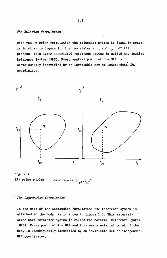
The Eulerian formuZation
With the Eulerian formulation the reference system is fixed in space,
as is shown in fiqure !.1 for two states- t 1 and t 2 - of the
process. This space-associated reference system is called the Spatial
Reference System (SRS). Every spatial point of the SRS is
unaabiquously identified by an invariable set of independent SRS
coordinates.
rP2 ----
Fig. I.l
SRS point P with SRS cooPdinates (r ,r ) pi p2
The Lagrangian formuZation
In the case of the Laqranqian formulation the reference system is
attached to the body, as is shown in fiqure !.2. This material
associated reference system is called the Material Reference System
(MRS). Every point of the MRS and thus every material point of the
body is unaabiquously identified by an invariable set of independent
MRS coordinates.
!.3
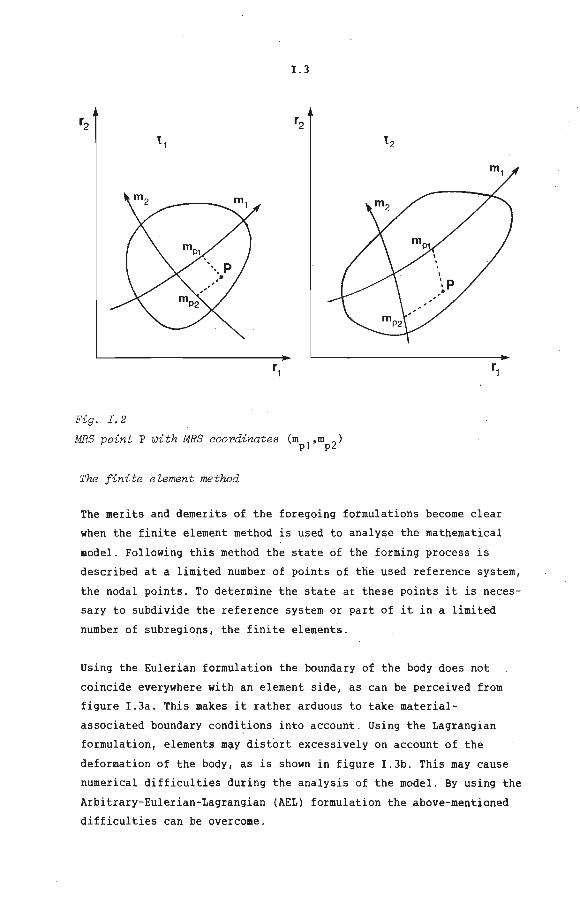
Fig. I. 2
MRS point P with MRS coordinates (mpl'mp2)
The finite element methad
The merits and demerits of the foregoing formulations become clear
when the finite element method is used to analyse the mathematica!
model. Following this method the state of the forming process is
described at a limited number of points of the used reference system,
the nodal points. To determine the state at these points it is neces
sary to subdivide the reference system or part of it in a limited
number of subregions, the finite element~.
Using the Eulerian formulation the boundary of the body does not
coincide everywhere with an element side, as can be perceived from
figure I . 3a. This makes it rather arduous to take material
associated boundary conditions into account. Using the Lagrangian
formulation, elements may distart excessively on account of the
deformation of the body, as is shown in figure I.3b. This may cause
numerical difficulties during the analysis of the model. By using the
Arbitrary-Eulerian-Lagrangian (AEL) formulation the above-mentioned
difficulties can be overcome.

I . 4
t, '[2
/"' -~ / /
V J /
V
V a V /
~ ~ / V
1\. I'--"' ""'- V -
Fig . . r. 3
Element mesh, using the Euler>ian (a) and the Lagroangian (b) tormulation
The Arobitroaroy-Euler>ian-Lagroangian tormulation
The reference system tised in the AEL tormulation is not fixed in
space nor attached to the body, as is shown in figure !.4. This non
associated ieference system is called the Computational Reference
Systea (CRS). Every point of the CRS is unaabiguously identified by
an invariable set of independent CRS coordinates .
The fact that the position of the CRS points is not given, yet can

!.5
be freely determined provides much freedom in formulating the
mathematica! model. The CRS can be f:i.xed in space, which leads to an
Eulerian formulation, or can be attached to the body, thus leading to
a Lagrangian formulation . The position of the CRS points can also be
changed continuously and in a prescribed manner during the simulation
of the forming process . The CRS point positions can also occur in the
mathematica! model as unknown variables. In that case the model has
to be extended by considering a so- called CRS determination process
simultaneously with the forming process.
Fig. I. 4
CRS point P with CRS coordinates (gpl' gp2)
In the mathematica! model of a forming process accordi ng to the AEL
formulation, both the CRS and the MRS are used . The AEL formulation
requires that there is an unambiguous conneetion between these two
reference systems in every state . The freedom to choose the position
of the CRS points is thus limited in the sense that each CRS point
always coincides with one and only one , though not always the same
MRS point and vice versa. This means that the boundary of the CRS
always coincides with the boundary of the body to be deformed . Thus,
when using the finite element method, all sorts of boundary

!.6
conditions can easily be taken into account. At the same time the
nodal point positions can be prescribed or determined in a CRS
deteraination process, in such a way that the dimension and the
geometry of the elementsis appropriate (see figure !.5).
r, ~
Fig. I. 5
Element mesh, using the AEL fo~Zation
The AEL fo~Zation in titerature
The AEL formulation, tagether with the finite difference or the
finite element method, is frequently employed to simulate processes
in gasses and fluids and processes with fluid-structure interaction .
- Hirt et al. (1972), Pracht (1974), Stein et al. (1976), Belytschko
& Kennedy (1978), Donea (1978), Dwyer et al . (1980), Hughes et al.
(1981), Kennedy & Belytschko (1981), Donea et al. (1982) -. Very re
cently the AEL formulation, tagether with the finite element method,
has been used to simulate forming processes - Huetink (1982) -. As
well in the Eulerian as in the Lagrangian formulation, so-called
rezoning methods are used, where the nodal point positions are
adjusted, if necessary, in a rather ad hoc manner - Gelten & De Jong
(1981), Roll & Neitzert (1982) -
II . 1
II An AEL formulation for continuurn mechanics
. 1 Introduetion
.2 Geometrie and kinematic quantities
.3 Stress tensors
. 4 The equilibrium equation and the principle of weighted
residuals
.5 A constitutive equation for time independent elasto
plastic material behaviour
II.1 Introduetion
When employing the Arbitrary-Eulerian-Lagrangian (AEL) formulation to
the simulation of roetal forming processes, two sets of independent
variables are used: the coordinates in the Computational Reference
System (CRS) and the coordinates in the Material Reference System
(MRS), respectively, the so-called CRS and MRS coordinates. Various
geometrie quantities can be defined at every point of these reference
systems. Considering the change of these geometrie quantities during
a state transition leads to the definition of various kinematic
quantities . The kinematic quantities which refer to a point of the
MRS describe the deformation of the material. In every state there is
an unambiguous relation between the CRS and MRS coordinates. Sectien
II.2 deals with the geometrie and kinematic quantities and the
relation between CRS and MRS coordinates.
The deformation provokes stresses in the material. The stress state
in an MRS point is represented by means of a stress tensor. In sec
tien II . 3 two stress tensors are introduced.
If inertia effects are neglected the internal stresses and the
external loads must constitute an equilibrium state. This means that

!!.2
at every MRS point the stress tensor and the external load vector
have to satisfy an equilibrium equation. This equation is presented
insection !!.4. Subsequently an integral formulation is introduced
which is equivalent to the equilibrium equation and very suitable for
determining an approximated solution.
The stresses in the material and the deformation which causes them
must satisfy a constitutive equation. In section !!.5 a constitutive
equation for time independent, elasto-plastic material behaviour is
presented.

II. 3
II.2 Geometrie and kinematic quantities
The MRS coordinates
Geometrie quantities
Kinematic quantities
The boundary
Geometrie quantities at the boundary
Kinematic quantities at the boundary
Deformation quantities
Rigid body rotation and co-rotationaZ quantities
The CRS coordinates
Geometrie quantities
Kinematic quantities
The boundary
Geometrie quantities at the boundary
Kinematic quantities at the boundary
The reZation between MRS and CRS coordinates
The MRS coordinates
Each partiele of a three-dimensional body can be identified unam
biguously by a set of three independent MRS coordinates m1, m2 and
m3
, which can be taken as elements of a column m. The columns m of
all MRS points are the elements of an invariable set M. In state T
the position vector p of MRS point m with respect to a fixed spatial
point, the origin, is
.. p
.. x(m, T) (II .2.1)
In state T the function ~. which is unique, continuous and
sufficiently differentiable, can be considered as a mapping .. x : M .. V(t), where V(t) is thesetof end points of the position .. veetorspof the MRS points. A subset of V(T), containing the end
points of the position veetors p = x(m,T), with mEM and m. is J
constant for j f i, is called the mi-parametric curve in state T .
The end point of every position vector p is situated on three
different parametrie curves (see figure II.2.1).
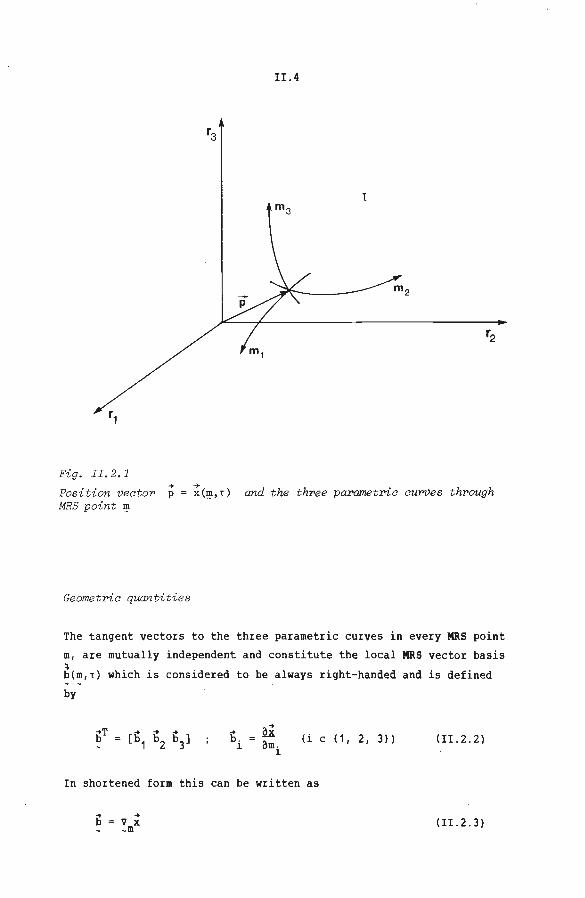
II.4
l
Fig. II. 2. 1 -+ -+
Pos ition veetoP p x(~,T) and t he thPee paPametrie curves thPough MRS point ~
Geometrie quantities
The tangent veetors to the three parametrie curves in every MRS point
m, are mutually independent and constitute the local MRS vector basis ~ b(m,t) which is considered to be always right-handed and is defined
by
b. 1
(i c {1, 2, 3}) (II.2.2)
In shortened form this can be written as
.. V x ~m
(11.2.3)
II. 5
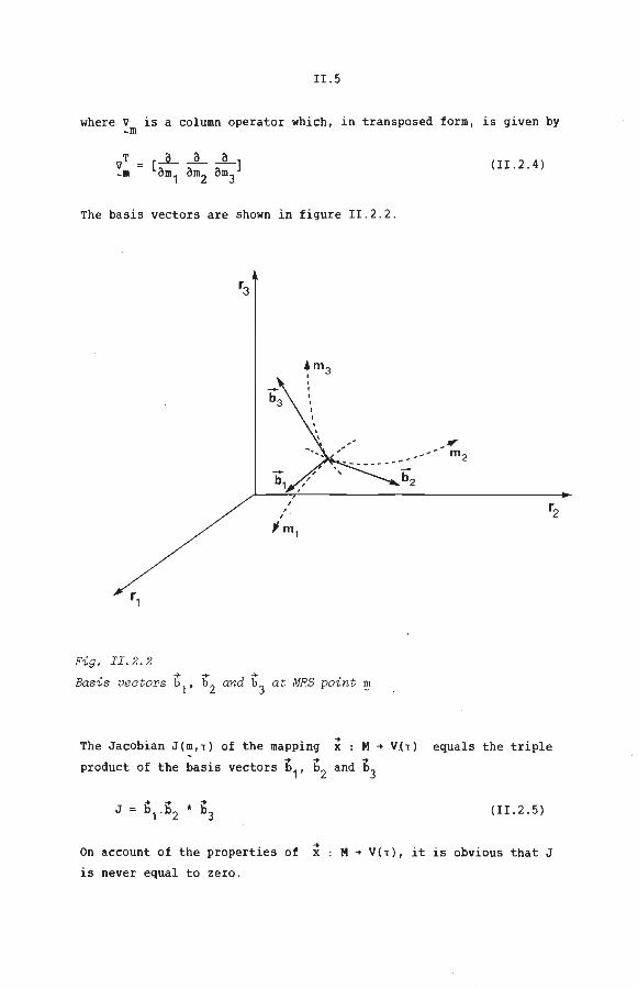
where V is a column operator which, in transposed form, is given by ~m
The basis veetors are shown in figure !!.2.2.
Fig. II. 2.2
, I
fm 1
->- ->- ->-Basis veetors b
1, b
2 and b
3 at MRS point ~
The Jacobian J(m,t) of the mapping .. x M .. V(t) .. .. ..
product of the basis veetors b1, b2 and b3
J
(II.2 . 4)
equals the triple
(II. 2 . 5)
On account of the properties of
is never equal to zero.
.. x M .. V(t), it is obvious that J
II.6
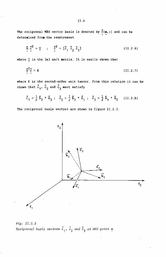
The reciprocal MRS vector basis is denoted by ~(m,t) and can be
determined from the requirement
I (II .2 .6)
where I is the 3x3 unit matrix. It is easily shown that
[ (II.2.7)
where [ is the second-order unit tensor. From this relation it can be .. .. .. shown that c 1, c2 and c3 must satisfy
1 b * b J 2 3 (II.2.8)
The reciprocal basis veetors are shown in figure II . 2 . 3.
Fig. II.2.3 + + +
Reciprocal basis veetors c 1, c2
and c3
at MRS point~

IL 7
Using the local reciprocal vector basis, the gradient operator can be
expressed in the column operator ~m
.. V
-+T c V ~ ~m
Kinematic quantities
,. .. v b.v ~m
(II.2.9)
In every state and at every MRS point the quantity A is defined and
given by A= a(m,t). The change of A at MRS point m duringa state
transition àt is called the MRS change of A and denoted by àmA
(II.2 . 10)
The MRS derivative of A is denoted by A and defined by
A (!!.2 . 11)
The velocity ~ of an MRS point is defined as the MRS derivative of
the position vector of that point
.. .. v x(m , T)
.. p (!!.2 . 12)
Using (II . 2 . 3) and (II.2 . 9) it is easily shown that for the MRS
derivate of b the following expression holds
~ .. .. .. b . (V V) (I I. 2.13)
With ~.bT find for ...
that I we c
.. ~- !v c
.. c V) (!!.2.14)
The tensor (V ~)c in the above expression can be decomposed into a
symmetrie part D and a skew- symmetric part ~. so that
D + !l -+T-+ b c [)
I I. 8
!l (II.2.15)
For the tensors[) and !l, called the deformation and rotatien rate
tensor, the next expressions hold
1 (~T~ .. T-+ 1 .. ~)c + .. .. [) + c b) {(V (V v))
2 ~ ~ 2 (II.2 . 16)
1 (~T~ .. T-+ 1 .. .. c .. .. g)
2 c b) 2
{(V v) - (V v)) (II.2.17)
For the MRS derivative of the Jacobian J we find
J J ~T-~ .. .. J(V .v) J tr(D) (II.2.18)
The boundary
An MRS point on the boundary of a three-dimensional body can be
identified both by the MRs- coordinates m and a set of two independent * * * coordinates m1 and m2, taken as the elements of a column m . The
* columns m of the MRS points on the boundary are the elements of a * set M . We assume that the boundary is always made up of the same MRS
* points and therefore the set M is invariable. In state t the .. * position vector p of MRS point m is
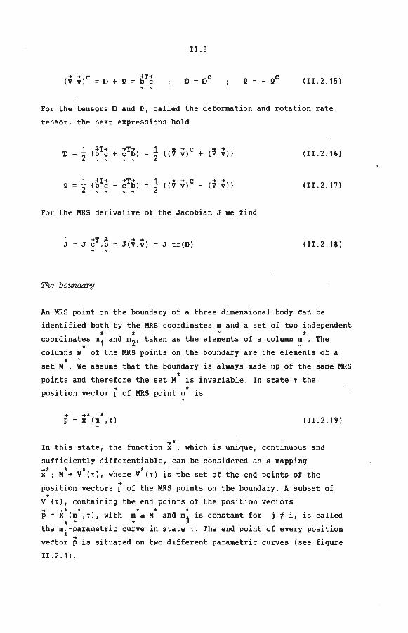
.. p .. * * x (m , t) (!!.2 . 19)
-+* In this state, the function x , which is unique, continuous and
sufficiently differentiable, can be considered as a mapping ~· * * * x : M .. V (t), where V (t) is thesetof the end points of the
position veetors p of .the MRS points on the boundary. A subset of * V (t), containing the end points of the position veetors
~ ~· * t * * p =x (m ,t), with meM and m. is constant for j f i, is called * ~ J
the mi-parametric curve in state t. The end point of every position
vector P is situated on two different parametrie curves (see figure
II . 2 . 4) .
r1
Fig. II.2.4
II. 9
Posi tion vector p = ;* (m * , T ) and the two parametrie curves t hrough . * -MRS boundary po-z-nt IE
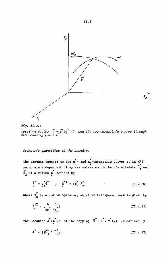
Geometrie quantities at the boundary
* * The tangent veetors to the m1- and m2-parametric curves at an MRS .. * point are independent . They are understood to be the elements b1 and
~* ~* b2 of a column b defined by
*
.... V x ~m
.. *T .. * ,.b*] b = [b 2 ~ 1
(11. 2 . 20)
where V is a column operator, which in transposed form is given by ~m
(11.2.21)
* * ~* * * The Jacobian J (m ,t) of the mapping x : M .. V (t) is defined by
* J (11.2 . 22)
!!.10
On account of the properties of ~* * * * x M ~V (t), J will never be
zero.
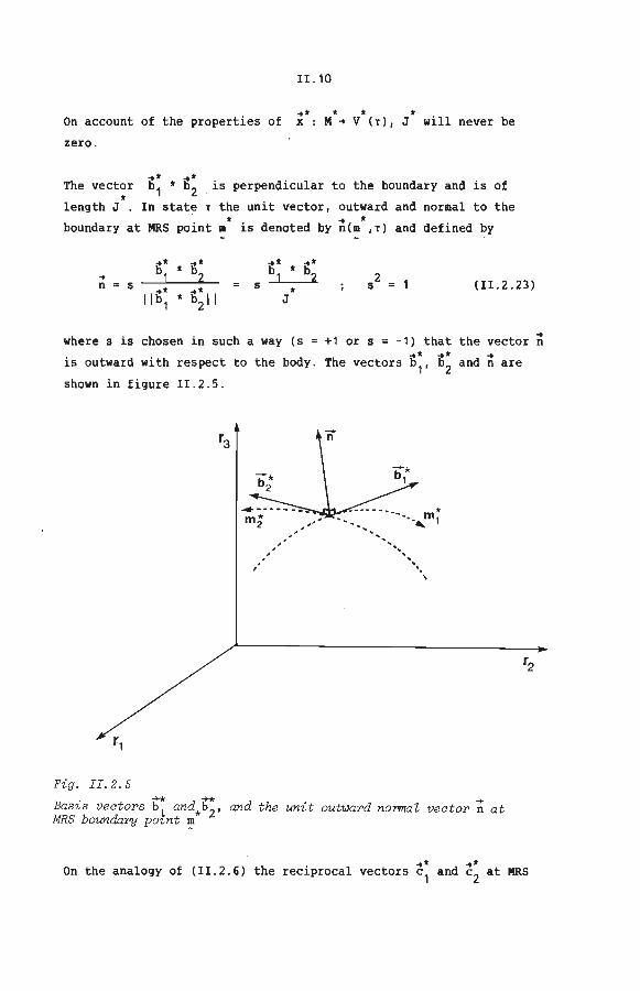
... ~* is perpendicular to the boundary and is of The vector b1 * b2
* length J In state T the unit vector, outward and normal to the * ~ * boundary at MRS point m is denoted by n(m ,t) and defined by
.. * * jj* jj* * .. * ~ bl 2 l b2 2 n = s
~* * jj * 11 s * s (11.2.23)
11 b1 2 J
where s is chosen in such a way (s = +1 or s = -1) that the vector n ~* ~* .. is outward with respect to the body. The veetors b1, b2 and nare
shown in figure 11.2.5.
Fig. II.2.5
' .. ,, '•.
\
• ~ -7-* -+ Bas~s veetors b 1 and*b2, and the unit outward no~az vector n at MRS boundary powt 1!_1
.. * .. * On the analogy of (11.2.6) the reciprocal veetors c1 and c2
at MRS

II. 11
* point m can be determined from
-.* -.*T -.*T ... -.* b . c I c [c1 c2] (II.2.24)
and
-.* .. ... .. c 1.n c 2 .n 0 (II.2.25)
where I is the 2x2 unit matrix. It can be shown not only that the
expression
-.*T-.* .. .. b c [ - n n (II.2.26)
-.* -.* satisfy must apply, but a lso that c1 and c2 must
-.* .§__ ... .. -.* L-. ... c1 * b2 * n c2 * n * b1
J J (II.2.27)
-.* * The gradient operator V , used at MRS point m to describe variations
of quantities at adjacent points on the boundary in state 1 , is
defined by
... V
-.*T * c V
~m
.. .. .. {([- n n).VI
Kinematie quantities at the boundary
(II.2.28)
Using (II.2.20), (II.2.28), (II.2.24) and (II.2 . 15), the next expres--.*
sion for the MRS derivative of b can be derived to give
With
s*
-.* c
..0* c
~* -+*-+* ... .. .. .. ... b . (V V ) b .{([ - n n) . (V V ))
l* .. .. + ll)cl b . {([ - n n) . ([)
.. *T .b I we find for
.... c
-+* -+*-+* c c . (V V ) ... * ... -+* c C .{(V V) .([
.. .. n n) I
:J* c . { ([) + 11) • ( [
.. .. n n)J
(II.2.29)
(I I. 2 . 30)
II. 12
* For the MRS derivative of the Jacobian J we find
. * J
* .. *T .0* J c .b * ~· -t* J (V .V )
Deformation quantities
* J ([ .. .. n n) :D (II.2.31)
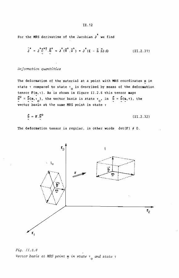
The deformation of the material at a point with MRS coordinates m in
state T compared to state T0
is described by means of the deformation
tensor F(m,T). As is shown in figure II.2.6 this tensor maps .. 0 .. - ' .. b = b(m,T ), the vector basis in state T , in b - - - 0 0
.. b(m,t), the
vector basis at the same MRS point in state T
(II.2 . 32)
The deformation tensor is regular, in other words det(F) 1 0.
Fig. II.2.6
. . .
;-. . . . . . . . · . .
!
........
.. .................... ..
Vector basis at MRS point m in state T and state T 0

II. 13
The basis veetors b0 span a volume àV0 = lb~.b~ * b~l and the basis
veetors b span àV = lb 1.b2 * b31. It is easily shown that the next
relation between the infinitesimal material volume elements dV and
dV0 must apply
dV = det(~) dV0 (!!.2 . 33)
From this relation we can conclude that det(~) > 0. The determinant
of ~ is called the volume-change factor ö
ö det(~l (!!.2.34)
Using -.T-. b c = [, ~ can be written as
~ +T-.o [~oT(V ~l]c = (Vo~ 1 c b c
~ ~m (!! . 2.35)
-1 the inverse of and ~ , ~. as
~-1 boT~ -.T -.o c ~c (V x l] ~ ~m
(_. -.o c V x ) (!!.2.36)
It can easily be shown that, for the MRS derivative of~ and ~- 1 , the
next expressions apply
~ ~T~o = (Vo~ 1 c = (V ~)c.~
F-1 boT~=_ ~-1 .(V ~lc
(!!.2.37)
(I I. 2. 38)
On account of (!! . 2.35) the relation between the two infinitesimal
material line elements d~0 d~(m,t ) and d~ = d~(m,t) is ~ 0
-. -.o dx ~.dx (!!.2.39)
With ~0 and ~ as the unit veetors in the direction of d~0 and d~, and
ds0 and ds, the lengths of these line elements, we can write, for the

II. 14
length-change · factor À
À dL: ds 0
lliill ds0
(II.2.40)
Using (!!.2.39) we find
1 IIIF. ~0 11
.. 0 c .. 0 -À = {n .IF .IF.n 12 (II.2.41)
The above is illustrated in figure !!.2.7.
r3
lo 1
'!I+ d '!I
'!'-- '!I + d '!I dx-...... > I F '
ds0
/ -o
-dx - ~ / /
" /
/ ds
'!I '!I /
Fig. II.2.7
The infinitesimal material line elements: -+o -+ o -+ o o-+o -+ -+ -+ -+
dx = p(~+d~,T ) - p(~,T ) = ds n ; dx = p(~+d~,1) - p(~,1) ds n
According to (II.2.41) the total deformation of the material at an
MRS point m can be described by the so-called stretch tensor U,

II .15
defined by
u u (11.2.42)
On account of this definition of U, a tensor R can be defined in such
a way that the following decomposition of F applies
F = IR.U Rc.IR = [ det(IR) +1 (II.2.43)
Because of the requirements which IR has to meet, we can conclude that
IR de~cribes a rigid body rotation of the material at MRS point m. The
above decomposition is called the polar decomposition of F and the
tensor IR the rotation tensor in the polar decomposition of F.
The Green-Lagrange strain tensor E is defined by
~(Fc.F- [) (11.2.44)
For the deformation rate tensor D and the rotation rate tensor ~ we
can write
D + ~ (II.2.45)
The MRS derivative of the volume-change factor ~ can be expressed
in I> as
. -1 ~ tr(F.F ) ~ tr(D) (11.2.46)
-o*o -o*o In state t 0 two independent veetors b1 a~~ b2 ~~0the .. ~~undary of a
three dimensional body span a surface 6V I lb1 * b2 I I . The ~* -+*
t, b1 and b2 , span a surface
factor is defined as
corresponding veetors in state * ~* -+* 6V llb 1 * b211. The surface-change
* ~ (II.2.47)
II .16
where dV* and dV*o are infinitesimal material surfaces. After some . * manipulations we arrive at the following expressions for 6 and its
MRS derivative' Ö *
(11.2.48)
. * 6
-.o ·-1 -c -.o det(IF) [cV ~> IIIF-c . ~0 11 + n .f .lF.If .n ] (~!.2 . 49)
IIIF-c-~0 11
Rigid body rotation and eo-rotational quantities
Besides the rotation tensor R in the polar decomposition of IF there
are many tensors r which meet the requirements
det(T) +1 (II. 2. 50)
and also describe a rotation of the material in state T compared to
state T0
. 1f we assume D = V, it is possible to introduce a rotation
tensor, which unambiguously describes the rotation of a material line
element d~ in state T compared to state T that is o'
d~(m,T) l'(m,T) dx<m,T > - 0
For the MRS derivative we obtain
.:. dx(m, T) T(m,T) dx<m,T >
- 0
(1!.2.51)
(1!.2.52)
Using the deformation rate tensor D and the rotation rate tensor 0,
we write generally
.:. dx(m,'T) {D(m,T) + O(m,T)}
In view of the assumption D V, this expression becomes
.. dx(m,T) O(m,T)
(1!.2.53)
(II.2 . 54)
II. 17
From (!!.2.51), (!!.2.52) and (!!.2.54) the following differential
equation results
U' tL I' (!!.2.55)
with the initial conditions
I' [ at (!!.2.56)
On the analogy of the polar decomposition, Nagtegaal & Veldpaus
[21] decompose the deformation tensor F to give
f = I'.F (!!.2.57)
where F is called the co-rotational deformation tensor which is
invariant to the rotatien described by U'. The co-rotational defor
mation rate tensor is defined by
(!!.2.58)
If it is assumed that D is constant during the state transition
it can be shown that
must hold
[) 1 • --~ t-l
0
- 1- ln(IF) t-1:
0
I' = IR and that the next expression for D
(!!.2.59)
The tensor ~ is called the logarithmic strain tensor.
The CRS coordinates
Employing the Lagrangian formulation, the Material Reference System
(MRS) is used, that is, every quantity is understood to be a function
of the MRS coordinates m. The Computational Reference System (CRS),
which can move independently of the material, is introduced into the
AEL formulation in such a way that each MRS point coincides with only
one CRS point and vice versa in every state.

I!. 18
Each CRS point can be identified unambiguously by a set of three
independent CRS coordinates g1, g2 and g3, which can betaken as
elements of a column g. The columns g of all CRS points are the
elements of an invariable set G. In state T the position vector p of
CRS point g is
.. p (I!. 2 . 60)
In state T the function x, which is unique, continuous and suf
ficiently differentiable, can be considered as a mapping
x : G-+ V(t), where V(t) is the set of end points of the position
veetorspof the CRS points in state T. A subset of V(r), containing
the end points of the position veetors p = x(g,T), with ge G and
gj is constant for f i, is called the gi-parametric curve in state
t. The end point of every position vectorpis situated on three
different parametrie curves.
In the preceding part of this sectien we introduced various quan
tities as a function of the MRS coordinates. In the succeeding part
we introduce similar quantities as a function of the CRS coordinates.
Geome trie quantities
The local CRS vector basis p(g,T) is chosen right-handed and defined
by
.. V X _g
where V is a column operator, given by -g
The Jacobian J(g,T) of the mapping .. x
(11.2.61)
(II.2 . 62)
G -+ V(t) equals the triple
product of the basis veetors p1, p2 and p3, so that
J (II.2 . 63)
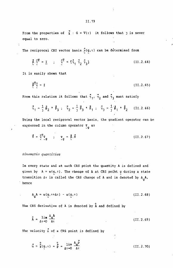
From the properties of
equal to zero.
.. x
II. 19
G .. V(T) it follows that J is never
The reciprocal CRS vector basis ~(g,T) can be d~termined from
.. ..T ~-'1 I (II.2.64)
It is easily shown that
[
From this relation it follows that ~ 1 , ~2 and ~ 3 must satisfy
1 .. .. J ~2 * ~3
1 ... .. J ~ 1 * ~2 (II.2.66)
Using the local reciprocal vector basis, the gradient operator can be
expressed in the column operator V as ~g
.. ..T V 'I V
- ~g
Kinematic quantities
V ~g
(II.2.67)
In every state and at each CRS point the quantity A is defined and
given by A= a(g,T). The change of A at CRS poibt g duringa state
transition àT is called the CRS change of .A and is denoted by à A, g
hence
à A a(g,T+àT) a(g,T) g
The
The
CRS derivative
0 lim A àT .. Û
velocity ~
0 .. ..
à A _g_
àT
of
u x(g,T)
0
of A is denoted by A and defined by
a CRS
0 ..
point is
.. lim ~ p
tn .. o àT
defined by
(II.2.68)
(II.2.69)
(II.2.70)
II .20
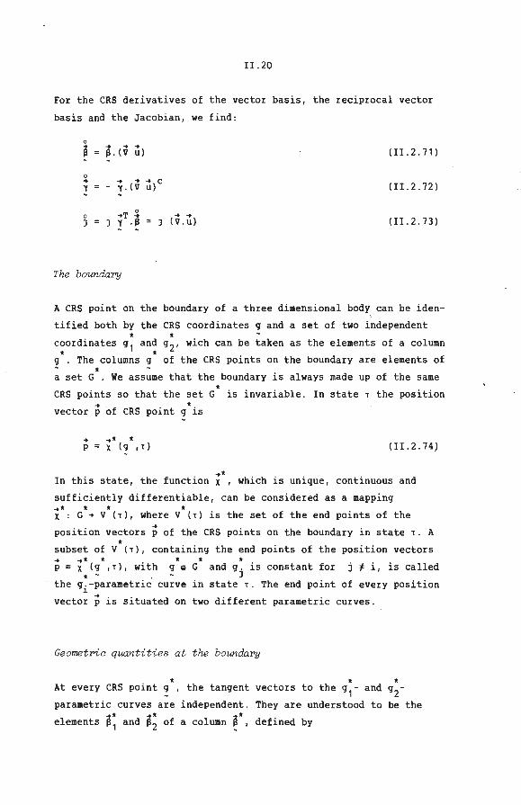
For the CRS derivatives of the vector basis, the reciprocal vector
basis and the Jacobian, we find :
0
~
0 .. "Y
0
J -.T ~
J "Y . IJ
The boundary
(II .2. 71)
(II.2.72)
(II . 2 . 73)
A CRS point on the boundary of a three dimensional body can be iden
tified both by the CRS coordinates g and a set of two independent * * coordinates g 1 and g2, wich can be taken as the elements of a column
* * g . The columns g of the CRS points on the boundary are elements of * a set G . We assume that the boundary is always made up of the same
* CRS points so that the set G is invariable . In state 1 the position
vectorpof CRS point g*is
.. p -.* * x (g ,, ) (II.2.74)
. .... . . In this state, the funct~on x , wh~ch ~s unique, continuous and
sufficiently differentiable, can be considered as a mapping .... * * * x : G .. V (l), where V (1) is thesetof the end points of the
position veetorspof the CRS points on the boundary in state 1. A * subset of V (1), containing the end points of the position veetors
... .... * * * * p =x (g ,,), with ge G and g. is constant for j I i, is called * - . J
the gi-parametric curve in state 1. The end point of every position
vector p is situated on two different parametrie curves.
Geometrie quantities at the boundary
* * * At every CRS point g , the tangent veetors to the g1- and g
2-
parametric curves are independent. They are understood to be the
~* ~· ~· elements p1 and p2 of a column ~ ., defined by

II. 21
f * .. * fT [a~ a;1 V X
~9 (!!.2 . 75)
* where the column operator V is given by
~g
v*T [~~] ~g ag
1 ag
2
(!! . 2 . 76)
* * ~* * * The Jacobian J (g ,T) of the mapping x : G .. V (T) is defined by
/ = 11 a~ * a; 11 (!!.2 . 77)
.. * The unit vector, outward and normalto the boundary; v(g ,T), can be
defined by
.. V * s
-;:t* ~* p * p 1 2
:t* * -+* * 111 p2
s *
* * where s is chosen in such a way (s
~ is outward compared to the body.
*2 s
* +1 or s
(!!.2 . 78)
-1) that the vector
~* ~* The reciprocal veetors 1 1 and 12 can be determined from
a* .. *T .. *T -+* .. * ·1 I 1 = [11 12] (!!.2.79)
and
-+* .. ..* .. 11. V 12 . v 0 (!!.2.80)
The expression
fT1* .. .. [ - V V (!!.2.81)
applies. The -+* and .. *
satisfy veetors 11 12 must
* * .. * .L a2
.. .. * .L .. .. 11 * V 12 V * p1 * * (!! . 2.82)
) )

.II.22
... The gradient operator V at a CRS point g describes variations of
quantities at adjacent points on the boundary in state T and is
defined by
... V
.. •T * 'Y V _g
Kinematic quantities at the boundary
-+* -t* The CRS derivatives of a I 'Y and are:
~· -t* -t*-t* ... .. .. .. ... 13 a . <v u 1 a . { ([ - V v). (V u
~· -t* -t*-t* c ... .{(v ... Je. ([ 'Y 'Y • (V u ) - 'Y u
o* 0 -t* -t* • .. *Tp* J J 'Y (V .u )
) }
-
The relation between MRS and CRS coordinates
(II.2.B3)
(II.2.84)
.. .. V v)} (II.2.85)
(II.2.86)
In state T 1 MRS point m coincides with CRS point g. For the position
vector p of these points we have
.. p X(ID 1 T) x<g~T) (II.2.87)
Since the functions ~ and x are unique 1 two unambiguous functions x
and x exist~ so that
m = x(p 1 T) g X (piT) (II.2.88)
Bath functions are continuous and sufficiently differentiable. In
state T the coinciding MRS and CRS points are related to each other
by the expressions
ID = X (X ( g 1 T ) 1 T ) g x<x<m1Tl1tl (II.2.89)
In state t+àt CRS point g coincides with MRS point m+àm as is shown
in figure II.2.8.
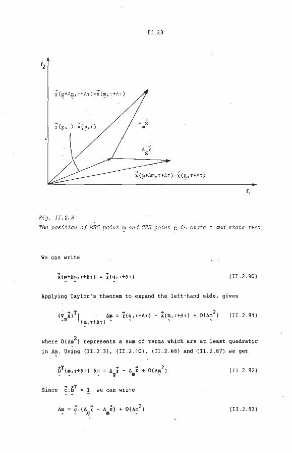
11.23
+ + X( g+~g, T +~T) =x(~,T+~T)
+ + x(g , T) =xÇ~,T)
+ + x(~+~~ , T +~T) =X(~ , T +~T)
r,
Fig. II.2 . 8
The position of MRS point m and CRS point g in state T and state T + ~T
We can write ; ·
(11.2 . 90)
Applying Taylor's theerem to expand the left- hand side , gi ves
. .. T (V x ) 1 · t.m ~ m (m,T+àT) •
(11.2.91)
2 where O(t.m ) represents a sum of terms which are at least quadratic
in t.m . Using (11.2.3), (11.2.10), (11.2.68) and ~(II.2 . 87) we get
i)T (m, T+àT) .. ..
0(t.m2J t.m à x - à x + g m (!1.2.92)
Si nee ~ . i)T I we can write
.. .. à ~) 0(àm2J àm c . (à x - +
~ _g m (!1.2.93)
II.24
In state T the value of the quantity A can be determined by employing
either or both of the functions a or a, so that
A a(m,tl a(g,Tl
The CRS change of A during the state transition àT is
à A a(g,t+àtl - a(g,Tl g a(m+àm,t+àtl - a(m,tl
(!!.2 . 94)
(II.2.95l
Expanding the first term of the right-hand side of the above expres
sion by means of Taylor's theorem, we find
a(m+àm,t+àtl a(m,t+àtl + (V alTI àm + O(àm2l (II . 2 . 96l .m (m,t+àtl •
This results in the expression for àgA given below,
à A a(rn,t+àtl - a(m,tl + (V alTI àm + O(àm2l g .m (m,t+àtl •
Substitution of (II . 2.93l gives
à A g
(II.2.97l
(II.2.98l
If the state transition is small, we may assume that the last term in
(II.2.98l can be neglected and that
(V All ~(V All (m,T+àtl (m,Tl
(!!.2 . 99)
This leads to the following relationship between the CRS _change à A g
and the MRS change àmA
à A g (!!.2.100)

I I. 25
11.3 Stress tensors
The Cauchy s t ress tensor
The co-rotat ionaZ Cauchy stress tensor
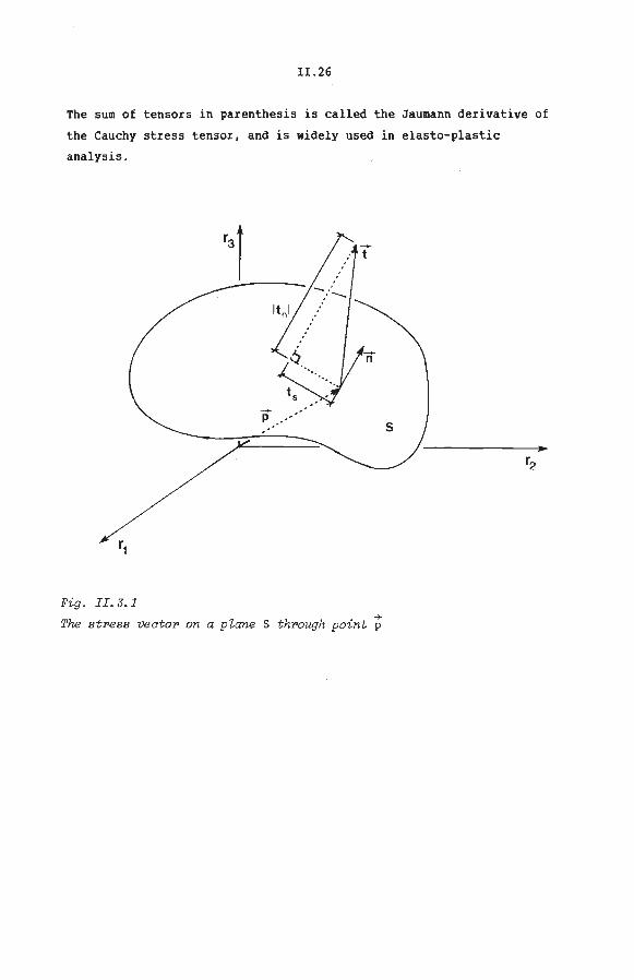
The Cauchy s t ress tensor
-+ -+ The stress vector t at MRS point p
-+ x(m,l) on a plane passing
through that point, is assigned to the unit vector ~. normal and
outward to that plane at point p, by a transformation o(m,l) . This
transformation can be shown to be linear- Lai et al.(1978) - and is
called the Cauchy stress tensor. We can write
-+ t
-+ a~ . n (!1.3 . 1)
-+ In figure 11 . 3 . 1 the stress vector on a plane S through pointpis
shown . The normal stress at p on the same plane is given by
t n
-+ -+ n . t
-+ -+ n . o.n
The magnitude of the shearing stress at p on the plane is
The co-rotationa Z Cauchy s tress tensor
.
(!1.3.2)
(Il . 3 . 3)
Following the introduetion of co-rotational kinematic quantities in
section II.2, the co-rotational Cauchy stress tensor G(m,l) is
defined by
(1!.3.4)
Using I' ~.1' we find for the MRS derivative of G
(1!.3 . 5)
II.26
The sum of tensors in parenthesis is called the Jaumann derivative of
the Cauchy stress tensor, and is widely used in elasto-plastic
analysis.
p
Fig. II.J.l
The stress vector on a pZane S through point t
II . 27
11.4 The equilibrium equation and the principle of weighted
residuals
The equi l ibrium equatian: di ffer en t i a l f arm
The equilibrium equatian: i ntegra l f arm
The equilibrium equation: differential f arm
Assuming that inertia effects are negligible, it follows from the
momenturn and mass conservation laws that in every state and at each
material point the next equilibrium equation must be satisfied
-+ -+ (V . u). + q
-+ VxeV(r) (II. 4.1)
The vector q represents the body force per unit volume in state t.
From the moment of momentum conservation law it follows that the
Cauchy stress tensor is symmetrie, hence
c ID = 1D
-+ V x'" V(t) (!!.4. 2)
Since each material point and thus each MRS point always coincides
with one single, yet not necessarily the same, CRS point, equations
(11.4.1) and (11.4.2) have to be satisfied at each CRS point in every
state t. Simultaneously the stress distribution and the deformation
have to satisfy the constitutive equation, the strain-displacement * * relationship, the kinematic boundary conditions at V cV and the
* * * .. r dynamic boundary conditions at V \V , where V is the coincident
P r boundary of CRS and MRS. Since, generally speaking, an exact solution
of the above equations cannot be found, we shall try to determine an
approximated solution. Equations (11 . 4 . 1) and (11.4.2) are not very
suitable for this purpose and thus an integral formulation is
introduced.

11.28
The equiZibPium equation: i n t egraZ farm
According to the principle of weighted residuals, the equilibrium
equation (11.4.1) is equivalent to the requirement that the integral
equation given below is satisfied in every state T for every al -.. lowable weighting function w(g,t)
I ~.[(v.~> + q) dV V(t)
0 (11.4.3)
The weighting functions ~ have to meet certain requirements, which
will be the case, if these functions are piecewise continuous (see
Zienkiewicz (1977)).
After choosing special weighting functions ~. equation (11.4 . 3) can
be used to determine approximated solutions for the equilibrium
equation. To relax the requirements as regards ;, the term ~.(9.~) in (11.4.3) is integrated by parts. This requires the weighting
function to be piecewise differentiable. Applying Gauss' law and
using ... .. t = n . ~, we arrive at
I (v ~lc:~ dV V(t)
I ~ . q dV + V(t)
•
I • V (t)
..... w.t • dV (II .4 . 4)
Since the integrals over V(t) and V (t) are extremely difficult to • evaluate, the integrations are carried out over the sets G and G
• With dV = J dG, dV
becomes
.. T-+ I (V W) 1 ' ~ J dG G ~g ~
where • and J
• • J dG and the above equation
~ ~ ~ ~* * * I w.q J dG + 1. w.t J dG (1!.4 . 5) G G
is the Jacobian of the-mapping x : G .. V(t) -t* * * .the Jacobian of the mapping x : G .. V (t).

I!. 29
II.S A constitutive equation for time independent elasto-plastic
material behaviour
A constitutive equation f or e l as t ic material behaviour
Elasto-plastic materia l behaviour
The yield condition
The decomposition of t he def ormation rat é t ensor
The MRS derivative of the his t ory parameters
A cons t i tuti ve equation fo r time independent e las t o-plas t ic
mat erial behaviour
A consti tuti ve equation for elastic mat erial behaviour
If the material behaviour at an MRS point is purely elastic , the MRS
derivative of the co-rotational Cauchy stress tensor and deformation
rate tensor must satisfy the next constitutive equation
(II.5.1)
In 9eneral the fourth-order elastic material tensor 4ê is a function
of the stretch tensor U, compared to the stress-free state, and a set
H, containin9 history parameters, which do not chan9e durin9 purely
elastic deformation (for detailed discussion of 4ê see for instanee
Hutchinson (1978) and Nagtegaal & De Jong (1980)) . In this report we 4.
assume, as is usually done, that r is constant at an MRS point . This
tensor is invertible and, owing to the symmetry of i, left. 4.
symmetrical. On account of the symmetry of D, ~ may be chosen ri9ht-
symmetrical.
Elasto-plastic mat erial behaviour
It is assumed that, if the material behaviour at an MRS point is
elasto-plastic, the MRS derivative of the co-rotational Cauchy stress
tensor and the co-rotational deformation rate tensor are related by a
II.30
constitutive equation similar to (11.5.1)
4 .. L:D (II . 5.2)
4. To determine the fourth-order tensor L, the first thing to do is to
introduce a yield condition. After this the deformation rate tensor D
is written as the sum of a tensor De, representing theelastic
deformation, and a tensor DP, representing the plastic deformation.
The next step is to write DP as a tunetion of D. For this purpose an
associated flow rule is assumed and assumptions are made concerning
the MRS derivative of the history parameters. Because of the symmetry
of i and D the tensor 4i is left-symmetrical and may be chosen right
symmetrical.
The yield condition
It is assumed that for plastic defórmation to occur at a material
point with MRS coordinates m, it is necessary that a scalar tunetion
of the co-rotational Cauchy stress tensor i(m) has reached a certain
limit value. This value depends on the deformation history of the
material at MRS point m, which is characterised by a set of history
parameters H, which change during plastic deformation only. Hence,
plastic deformation can occur only if the yield condition given below
is satisfied
f(i,Hl 0 (II.5.3)
The value of f(i,H) will never exceed zero, so that, during plastic
deformation the consistency equation
f 0 (II.5.4)
must be satisfied. The symbol * denotes a multiplication if H is a
scalar, a dot product if H is a vector and a double dot product if H
is a second-erder tensor. We will now discuss D and H.
I I. 31
The deeomposition of t he def oTmation rate t ensor
Following Nagtegaal & De Jong (1980) the deforrnation rate tensor D is
written as the sum of a tensor De representing the elastic defor
mation, and a tensor ~p representing the plastic deforrnation. Tensor
De is defined by the following expression
(II . 5 .5)
The tensor oP is defined by
(II . 5. 6)
Combination of (!! . 5.5) and (!!.5.6) gives
(II . 5. 7)
It is assumed that the material behaviour during elasto-plastic
deforrnation obeys an associated flow rule , that is
ID• P = N af ~ om (II . 5 . 8)
If the "length" of ~ is denoted by 13 and its "direction" by the
normalized tensor ~. we get
(!!.5 . 9)
Substitution in (!! . 5.7) results in
4. . 4. G: :ID - Ç 11::~ (!! . 5.10)
The MRS derivat ive of the history paramet er s
It is assumed that the MRS derivative of the history parameters H is
a function of the co- rotational plastic deforrnation rate t ens or DP,

1!. 32
so that
k(~ 111) (II.5 . 11)
The function k is such that
H k(~ 111) ~ k(n) (II . 5 . 12)
A constitutive equation for time independent elasto- plastic material
behaviour
Applying ~ = P n the consistency equation (11.5.4) becomes
(II . 5 . 13)
Substituting (11.5.10) and (11.5.12) in (11.5.13) results in
4. • 4. 3f p n : ~:D - p ~ 111: ~:111 + ~ aH*k(n) = 0
For ~ we can solve
4 .• n : ~:D
4. 1 3f 111 : ~ : n - ~ aH*k(n)
(II . 5 . 14)
(II.5.15)
Substituting in (11 . 5 . 9) results in the relation between DP and D given below
4. n n : ~
4. 1 3f n : ~ : n - ~ aH*k(n)
:D (II.5.16)
Substi tution of (11 . 5 . 16) in (11 . 5 . 7) finally results in the
constitutive equation
4 . 4.
( 4 C. _ ---:----"~ .... • .. o_.n~·'-::"G:'---] 4. 13f ;[)
n: ~ : n - ~ aH*k(111)
4 •• IL:D (II.5.17)
III.1
III Discretisation
. 1 Introduetion
. 2 The incremental method
.3 The finite el~ment method
.4 Calculation of material-associated quantities
III.1 Introduetion
In order to determine the MRS change of the co-rotational Cauchy
stress tensor during a state transition, the constitutive equation
(II.5.17) has to be integrated. If, during the state transition AT,
the co-rotational deformation rate tensor D is not a known, explicit
function of the state parameter T, integration can not be carried
out. In that case an incremental method is employed, according to
which the state transition is effected in a number of steps, the
increments. The chosen. size of an increment must allow the assumption
that D is constant during that increment. Starting from a known state
T0
, the beginning of an increment, the change of all relevant quan
tities should be determined in such a way that the weighted residual
equation (II . 4 . 5) is satisfied for every allowable weighting
function, in state Te' the end of the increment. The change of a
quantity + during an increment is called the incremental change of +
and is denoted by A+, where A+ = +(Te) - +(T0
) = +e - +0. This
incremental method, which in fact is a discretisation of a state
transition, will be discussed in section III . 2. In literature the
method is also referred to as the incremental method of weighted
residuals.
Though it is usually impossible to satisfy (II . 4.5) in state 1 for e
every allowable weighting function, this equati on can be satisfied
for every weighting function in a confined class. In this way an
approximated solution for the equilibrium equation in state Te is
III.2
obtained. To handle integration over geometrical complex volumes and
boundaries and to obtain a good approximated solution, despite the
fact that a simple weighting function is used , the finite element
method is employed . According to this method the CRS is subdivided
into subregions of rather simple geometry: the elements . In every
element the weighting function and the incremental change of some
relevant quantities are interpolated between the values of these
quantities at a limited number of CRS points belonging to this
element, the element nodal points . Known and simple functions of the
CRS coordinates g are used for the interpolation. The finite element
method is discussed in section III.3.
To determine whether the accuracy of the approximated salution is
good enough and, if this is the case, to carry out the next incremen
tal calculation, certain material -associated quantities must have a
known value at various CRS points. Because the CRS is not material
associated, it is impossible to calculate these values directly. A
special method which is discussed in section III . 4 has to be used .

III. 3
III.2 The incremental method
Starting from the known state T0
, the beginning of the increment, the
incremental changes of the reciprocal vector basis ~' the Cauchy * ~
stress tensor m, the boundary load t , the Jacobians J of the mapping ~ * ~* * * x : G ~ V and J of the mapping x : G ~ V have to be determined
in such a way that in state Te' the end of the increment, the
equation
~ T~ I (V w) "1: u J dG G ~g ~
~ ~ ~ ~· * * I w.q J dG+ I* w.t J dG (!!!.2.1) G G
is satisfied for every allowable weighting function w. In addition to
the above weighted residual equation, the constitutive equation, the
strain-displacement relations and the kinematic and dynamic boundary
conditions have also to be satisfied .
We assume the body force per unit volume, q, to have a known value at
every point. The .quantities in (III.2.1) whose value is not known at ~ .... *
every CRS point in state T , are -y·, m, t , J and J . Each of these e ~
quantities can be written as a function of the incremental
displacements of either the CRS points àr the MRS points. In view of
(II.2.72), (II.2.73) and (II.2.86) we can write :
~ ~o ~ ~o ~o ~ T~o "1 "1 + à "1 "1 "1 • <v à x> "1
g~ ~ ~g g ~ (III.2.2)
0 àg]
0 o~oT . <v à x> J = J + J + J "1 ~ ~g g (III.2.3)
* *o * *o *o~*oT * ~ . J J + à gJ J + J "1 . <v à x>
~g g (!!!.2.4)
Further we can write
( III. 2. 5)
Since the Cauchy stress tensor is a material-associated quantity, the
CRS change àgm is expressed in the MRS change àmm in accordance with
expression (!!.2.98)
l:J. Gl g
III .4
(III.2 . 6)
where ~(l:J.m2 ) represents a sum of terms which are at least quadratic
in
(!!!.2.7)
this being the change of the MRS coordinates of the CRS point g
during the state transition l:J.T. We now assume the increment to be
taken so small that ~(l:J.m2 ) in (!!!.2 . 6) can be neglected and (V 111)
determined in state T . Thus we find for 111 that 0
(III.2.B)
applies. After integrating the constitutive equation (!!.5.17), l:J. 111 m
can be expressed in Amx, formally: Ama = f(Amx), which results in
0 f(Am~) .. .. .. ..
Gl = Gl + + A X· (V G!) - Amx. (V G!) g (III.2.9)
-+* write For t we can
-+* t*o -+* t*o + * .. .. t + A t f (Agx' Amx) g (!!!.2.10)
f . . -+* .. ..
where we also use a ormal relat1onsh1p between A t , A x and A x, g g m which will not be discussed further. Substitution of (!!!.2.2-4) ,
(III.2.9) and (III.2.10) in (III.2.1) leads to an expression in the .. .. unknown incremental changes Agx' Amx.
lil. 5
111 . 3 The finite element methad
Discretisation of the CRS
InterpoZation of various quantities
AssembZy of the eZements
Di scretisation of the CRS
Employing the finite element method the CRS is subdivided into
elements. In every state, element e (e e 11,2 , ... ,n)) consistsof the
same CRS points, which can therefore be identified by local CRS
coordinates ~· defined per element. The set of local CRS coordinates
of all CRS points of element e is called Ge. The CRS points of that
element, pertaining to the boundary of the CRS, constitute the set * Ge. The int'egrals in ( 1II. 2. 1) are written as a summation of
integrals evaluated for the individual elements
n .. T .. [ I (V w ) 1 : v J dG
e=1 G ~g e ~e e e e
n r I ~ .q J dG
e=1 G e e e e
(III.3 . 1)
According to (III.2 . 2-4), .. * ( II I. 2 . 9) and ( II I. 2 . 10) , ! e, Je, Je, CD e .. * and te can be expressed in the incremental displacements
.. llgxe and ..
llmxe .
InterpoZation of various quantities
The .second step in applying the finite element method is the inter
polation of various quantities in every element . To interpolate a
quantity + is to write + as a linear combination of a number of known
functions of the local CRS coordinates, the interpolation functions.
The parameters in this linear combination are the values of + i n a

III .6
limited number of CRS points, the element nodal;points. The inter
polation functions have to meet certain requirements as is discussed
by Zienkiewicz (1977).
The interpolation of the position vector of CRS point q of element e
reads as
(ÜI.3.2)
Here, ~(g) is a column containing the known interpolation functions
and ~eCtl a column containing the position veetors of the element
nodal points. The interpolation of the incremental CRS point
displacement follows directly from (III.3.2)
(III.3.3)
where à x is a column containing the incremental nodal point q~e
displacements. The incremental MRS point displacement is also
interpolated. In this interpolation, the interpolation functions and
the element nodal points used are identical with those used when .. interpolating àgxe' thus
.. à x (g)
m e ~ (III.3.4)
.. where column à x contains the incremental displacements of the MRS
m~e
points that coincide with the element nodal points in state T . 0
The interpolation of à i (g) implies the introduetion of an m e ~ . approximation. Finally, the weighting function ~ is interpolated
e
.. w (g)
e ~
T -. Ijl (g) w ~ ~ ~e
(III.3.5)
.. where ~e is a column containing the values of the weighting function
in the element nodal points.

III. 7
AssembZy of the eZements
Af ter substitution of (III.3 . 5) in (III.3.1) we find
n n .. -+T T T-+ -+T I Ijl dG [ w I (V "' ) '( .IJ J dG [ w qeJe e=1 ~e G ~9~ ~e e e e=1 ~e G ~
e e
n -+T -+* * * + [ w I*+ te Je dG
e=1 ~e G ~
e
With introduetion of the vector columns ..
and the ~1e
.. .. ..
.1 (à x , à x ) ~ e 9~e m~e
(III.3.6) becomes
I G
e
n -+T .. .. .. [ w .m
1 (à x ,à x )
e= 1 ~e ~ e 9~e m~e
and
n -+T .. .. .. [ w • r 1 (à x , à x l
e=1 ~e ~ e g~e m~e
.. :1e
After assemblin9 the elements in the usual way we find
-+T -+ -+ -+ w .m
1 (à x,à x)
~ ~ 9~ m~
-+T ... ... -+ w .r
1(à x,à x)
~ ~ 9~ m~
(III. 3. 6)
accordin9 to
(III.3.7)
(III.3 . Bl
(III. 3. 9)
(III . 3.10)
The columns in the above expression contain the values of the various
quantities in all the nodal points of the element mesh. The elements
of a column containin9 the element nodal point values, denoted by ~ , ~e
constitute a subset of the elements of the correspondin9 column w containin9 all the nodal point values. The requirement that (III.2 . 1)
is satisfied for all wei9htin9 functions, interpolated in every
element accordin9 to (III.3.5), implies that (III.3.10) has to be
satisfied for all possible nodal point values of w, thus for every
possible column ~- It is easily seen therefore that the incremental .. .. displacements à x and à x have to satisfy the set of vector equations
9~ m~
.. .. .. r
1(à x,à x)
~ 9~ m~ (III.3.11)
III.8
111.4 Calculation of material-associated quantities
The necessary use of a special methad
The follower points
Interpolation of material-associated quantities
The necessary use of a special methad
The solution process used to solve the set of vector equations
(III.3 . 11) will be discussed in chapter V. In this process a number
of approximated solutions for (III.3.11l are determined. To establish
the accuracy of an approximated solution, the extent to which this
solution really satisfies the set of equations must be determined .
This set as described in sectien III.J results from the assembly of
terms evaluated per element. To evaluate each of these terms, one has
to integrate over the element domain. This integration is done
numerically: the value of the integrand is calculated at the in
tegration points of the element, after which a weighted summatien of
these values is carried out. Some of these integrands are a function
of material-associated quantities, such as the Cauchy stress tensor
and its gradient. Since the integration points are CRS points, which
usually do not follow the material, it is not possible to determine
the value of this material-associated quantities directly.
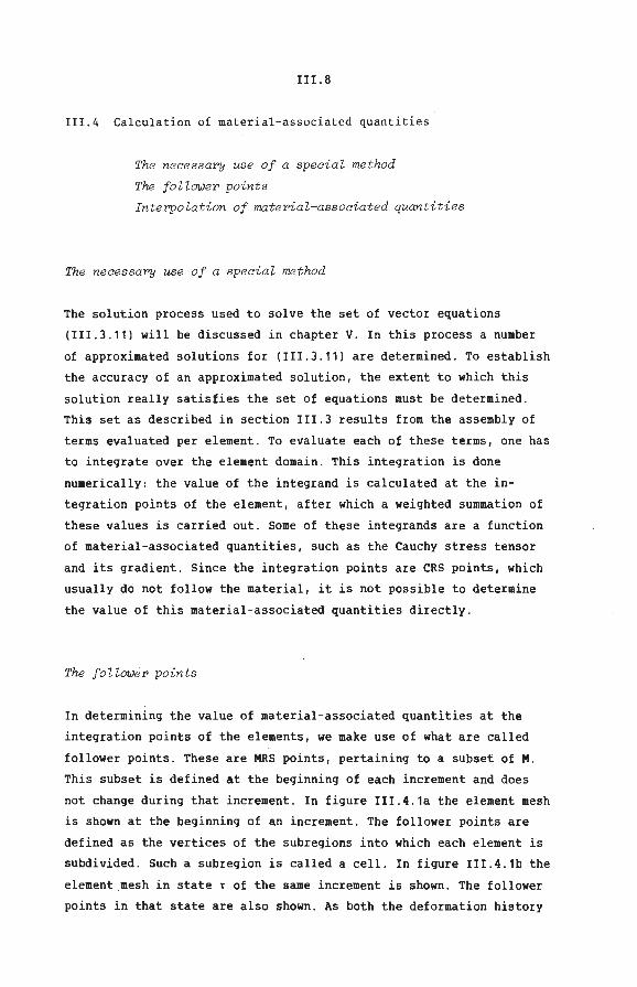
The f ollower points
In determining the value of material-associated quantities at the
integration points of the elements, we make use of what are called
follower points . These are MRS points, pertaining to a subset of M.
This subset is defined at the beginning of each increment and does
notchange during that increment . In figure III.4.1a the element mesh
is shownat the beginning of an increment . The follower points are
defined as the vertices of the subregions into which each element is
subdivided. Such a subregion is called a cell . In figure III . 4.1b the
element .mesh instatel of the same increment is shown. The follower
points in that state are also shown. As both the deformation history
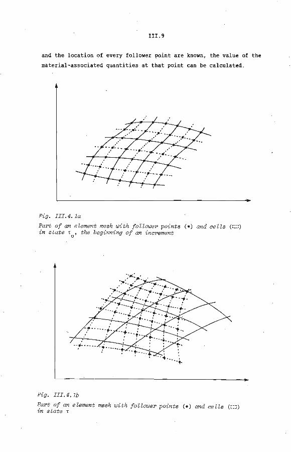
III . 9
and the location of every follower point are known, the value of the
material-associated quantities at that point can be calculated.
Fig. III. 4. la
Part of an eZement mesh with foZZower points ( • ) and ceZZs ('::~) in state T , the beginning of an increment
0
Fig. III. 4. 1b
Part of an eZement mesh with foZZower points (• ) and ceZZs (~: J) in state T
III. fo
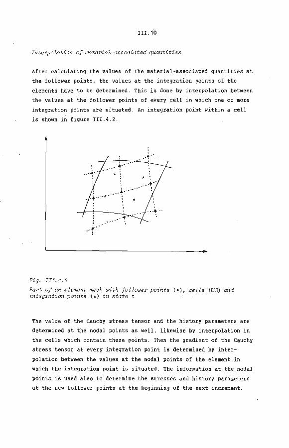
InteP,Do~ation of materia~-associated quanti ties
After calculating the values of the material-associated quantities at
the follower points, the values at the integration points of the
elements have to be determined . This is done by interpolation between
the values at the follower points of every cell in which one or more
integration points are situated . An integration point within a cell
is shown in figure III.4.2 .
0 ... ·o
............... 0
* :
*
.... .... .....
Fig . III .4. 2
Part of an e ~ement mesh wi t h f o Uowero points ( •), ce Us (~:.-:;) and i ntegroat ion points ( * ) in s tate T
The value of the Cauchy stress tensor and the history parameters are
determined at the nodal points as well, likewise by interpolation in
the cells which contain these points. Then the gradient of the Cauchy
stress tensor at every integration point is determined by inter
polation between the values at the nodal points of the element in
which the integration point is situated. The information at the nodal
points is used also to determine the stresses and history parameters
at the new follower points at the beginning of the next increment .
IV .1
IV The CRS determination process
.1 Introduetion
.2 The CRS determination process as a deformation process
IV . 1 Introduetion
For every nodal point there is one vector equation in the set
(III.3.11) . The equation fora nodal point contains the incremental
displacement veetors à x and à x, which can both be unknown. The g m number of unknowns in the set of equations may be up to twice the
number of equations which consequently cannot be solved . Specifying
the nodal point displacements and the boundary conditions must lead
toa solvable set of equations . The nodal point displacements must be
such that there is always a unique relationship between CRS and MRS.
Apart from this they may be chosen freely .
The freedom in specifying the nodal point displacements enables
certain requirements concerning element shape and element size to be
met. The shape affects the accuracy of the numerical integrations
carried out over the element. A good shape can be indicated for every
type of element. The element size affects the error which is possibly 0 • • ..
1ntroduced by 1nterpolat1ng àmx. If the number of elements and their
interconnection is constant, the optimum size of an element is not
known à priori, but depends on the condition of the material,
coinciding with the element in that state . The requirements as to
element shape may be incompatible with those affecting element size.
In that case a campromise between the requirements must be sought.
One known procedure used to specify the nodal point displacements is
the rezoning method (see Gelten ~De Jong (1981)). In the first step,
the rezoning, the free nodal point positions are determined at the
beginning of the increment to reduce the average deviation of the
optimum shape and siz·e of elements to a minimum, this average being
taken over all elements. The new nodal point positions can be
IV.2
determined automatically by means of a mesh generator - for instanee
Triquamesh (Schoofs et al . (1979)) -. In the second, the deformation
step, thesetof vector equations (III.3.11) is solved, with à x g~
chosen equal to à ; ,thus employing a Lagrangian formulation. The • m~
total incremental nodal point displacements are the summation of the
displacements during both the rezoning and the deformation steps.
Another procedure is presented in this thesis and used to specify the
nodal point positions . By this method the nodal point displacements
are understood to be the result of the deformation of a fictitious
material to which the CRS is associated and which progresses simul
taneously with the deformation of the real material with which the
MRS is associated. Todetermine this deformation, each element is
considered individually together with the fictitious material with
which it is associated . In the current state 1, the stresses in this
material are determined compared toa state 'f' in which the material
is stress-free and both shape and size of the element are optimal.
The load needed to effect the deformation from state 'f to state 1 is
determined so as to meet the requirement that the equilibrium
equation has to be satisfied in state 1, at every point of the
fictitious material. After assembling the elements, the total load on
the fictitious material is replaced by equivalent nodal forces.
Subsequently these forces are relaxed, after which the deformation of . .,
the fictitious material is effected by the internal stresses "and the
forces resulting from the coupling between CRS and MRS . Following the
procedure described in the preceding chapters, a set of vector
equations in the incremental nodal point displacements can be
formulated . This set is simultaneous with the set (III.3.11) because
of the relationship between CRS and MRS. Solving these simultaneous
sets gives à x and à~- The nodal point displacements, viz. the · g~ m~
deformation of the fictitious material, will be so as to minimize the
average deviation of the optimum element shape and size. When the
above method is used, the number of elements and their intercon
neetion does not change. This restrietion is not essential, yet makes
the method easier to describe and apply . In the next section the CRS
determination process is described . Symbols of quantities, which
refer to the fictitious material, are overlined .

IV.3
IV.2 The CRS determination process as a deformation process
The fictitious material
The optimum geometry of an element
The element nodal farces
Rela:ration of the nodal f arces
The fictitious material
The CRS is assumed to be associated with a fictitious material. To
describe the deformation of and the stresses in this material we use
the same quantities as in section II.2. The material behaviour is
assumed to be isotropie and elastic. On the analogy of (!!.5 . 1) we
can write
~ 4~ .=. "' = C:D
.:.
(IV. 2 .1)
where "' and D are the co-rotational Cauchy stress tensor and defor-
mation rate tensor respectively. The fourth-order elastic material 4.:.
tensor ~ is assumed to be constant.
The optimum geometry of an element
In every known state T we can indicate the optimum shape and size of
every element . This is described in detail in chapter V for one
particular element. In the state Tf' each element is successively
isolated from the element mesh and has the optimum shape and size.
The fictitious material associated with the element under con
sideration is stress-free (see figure IV.2.1). The deformation
tensor, which maps state Tf into state t, is denoted as Ff.
Without any restrictions to generality we may assume the co
rotational deformation rate tensor to be constant during this state
transition. Then, on the analogy of (II.2.59), we can write
(IV.2.2)

IV.4
D
Fi g. IV. 2.1
Part of an e lement mesh in state T and t he optimum geome try of one iso lat ed element in state T f
~f -f . where ~ is the logarithmic and E the Green-Lagrange strain tensor,
both considered with respect to the stat~ lf. Integrating (IV.2.1)
results in the co-rotational Cauchy stress tensor at a point of the
fictitious material in state T
(IV . 2 . 3)
If Rf is the rotation tensor in the polar decomposition of Ff, the
Cauchy stress tensor becomes
(IV.2.4)
The e lement nodal farces
For the fictitious material associated with one isolated element, the
d~formation from state 1f to state 1 can be effected by means of a

IV.5
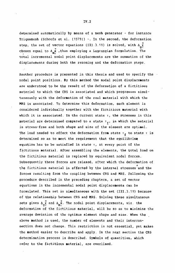
.. .. volume load q and a boundary load p, as is shown in figure IV.2.2a.
These loads must be so as to satis[y in state TI the equilibrium .. equation
.. -f + 3 at every internal point of the element. The (V.GJ ) q "'
equation -f ..
p = 111 .v must be satisfied at every point of the element
boundary. Assembling the thus loaded isolated elements produces the
body of fictitious material with which the CRS is associated. It is
obvious that this body has the same geometry as the body considered
in the forming process. It is loaded with volume loads and surface
loads as can be seen in figure IV.2.2b. These loads are replaced by
equivalent nodal forces, denoted by p, resulting in the situation
shown in figure IV.2.2c. These forces are determined per element and
those element nodal forces are denoted by Q . Using the method of ~e .
weighted residuals described insection II.4, and interpolating the
relevant quantities in each element as described in section III.3, it
is easily shown that the element nodal forces in state T are given by
expression
.. ~e
j.· .. ~~., ,·
~ .: ;
--f. ....... L ..... -···::'1: .. ····:.< .. ·{ , . . .... ! / tij;].:' "'
·+--.. ,! ..... - \ : ··:···--·" I q -: : ...- .........-
! ,;: .. ···:- I w .·. ,; .... "'"',. ,/ :
,•. ,' I
..... ......... _ .... -~
... ~· ..
: : ... -.~': __ ......... J ....... ·
·:
Fig. IV. 2. 2a + +
Volume laad q and boundary laad p on the fictitious material associated with one isolated element
(IV. 2. 5)
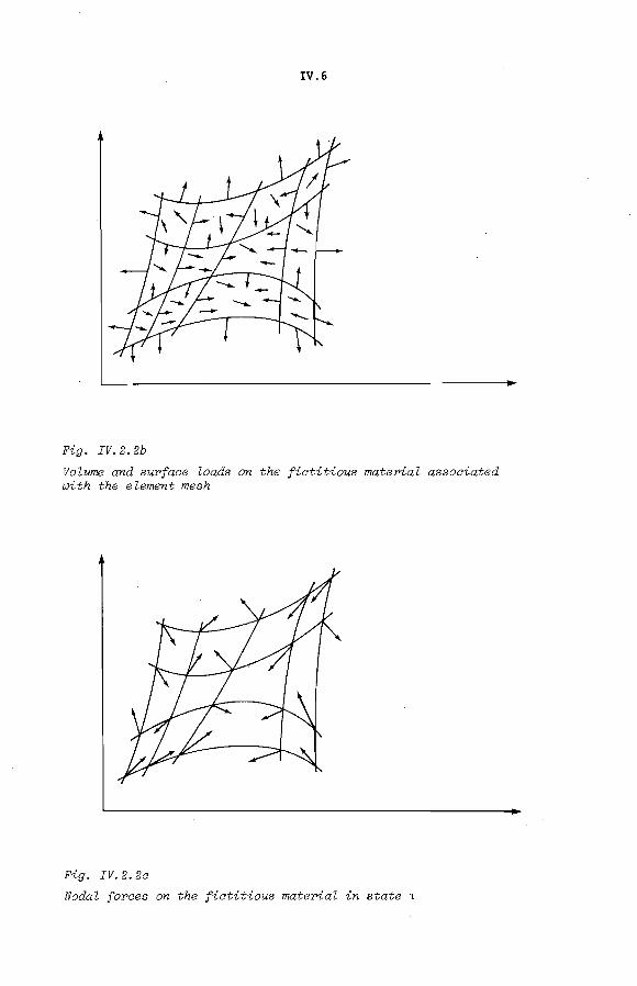
IV.6
Fig. IV. 2. 2b
Volume and surface loads on the fictitious material associated with the element mesh
Fig. IV. 2. 2c
Nodal foPces on the fictitious material in state 1
IV.7
Relaxation of the nodal f arces
Deformation of the fictitious material from state T to state Te' the
end of the increment, is effected by relaxin9 the nodal forces ~. In
state Te' the stresses resultin9 from this deformation, must satisfy
the equilibrium equation (V . Ü) = 0 at every point of the material.
In addition, the CRS boundary conditions must be satisfied. Usin9 the
method of wei9hted residuals and interpolatin9 the relevant
quantities in each element, results in the inte9ral equation 9iven
below, which is equivalent to the equilibrium equation and has to be
satisfied for every allowable wei9htin9 tunetion
n r .. T
w e=1 ~e
T T.. -I (V~ ) ~ .u J dG G ~9~ ~e e e e
(IV.2 . 6)
.. The nodal forces : 2 result from the couplin9 between CRS and MRS and
have a non-zero value only in those points where
Accordin9 to (III . 2.2) and (III.2.3), ~ and J ~e e
tunetion of the incremental displacements à x . 9 e
stress tensor can also be written as a tunetion
.. .. d
9x = dmx applies.
are written as a
Formally, the Cauchy .. of à x :
- .. ~e = f(à
9xe>· The incremental
9 e displacement à
9xe is interpolated
within each element accordin9 .. column ~2e by
relation (IV.2.6) becomes
n .. T .. .. r w .m
2 (à x >
e=1 ~e ~ e 9~ e
to (III . 3.3) . Definin9 the vector
(IV.2 . 7)
; .
(IV . 2.8)
Assemblin9 the elements in the usual way 9ives
.. T .. .. w .m2Cà x> ~ ~ 9~
(IV.2 . 9)
IV.8
The requirement that (IV .2.6) is satisfied for all weighting
functions, interpolated in every element according to (III.3 . 5) ,
implies that (IV.2 . 9) has to be satisfied for all possible nodal
point values of ;, thus for every possible column ;. The incremental
nodal point displacements à x have thus to satisfy the set of vector g, equations
(IV.2. 10)
V. 1
V The solution process
.1 Introduetion
.2 The iterative method
.3 Specification of the material behaviour
.4 Calculation of the stresses
.5 An iterative constitutive equation for time independent
elasto-plastic material behaviour
V.1 Introduetion
. The incremental nodal point displacements, à x, and the incremental q~ ..
displacement of the material in the nodal points, à x, must be deter-m~
mined in order to satisfy the followinq simultaneous sets of non-
linear vector equations pertaininq to the forming and CRS deter
mination processes, respectively:
.. .. .. m1Cà x,à x) ~ g~ m~
(V. 1. 1al
.. .. m2Cà xl ~ g~
(V.1.1b)
Additional coupling of these sets is caused by certain requirements
which the CRS and MRS displacements have to meet, including the
requirement that the CRS and MRS boundaries must always coincide. The
kinematic and dynamic boundary conditions must also be satisfied. It
is not possible to solve (V.1.1) directly because of the non
linearity of the equations. The solution procedure described in this
chapter, is known as th.e iterative method.
When the iterative method is used, a number of approximated solutions
for (V.1.1) is determined. The approximation for the exact value of
an incremental change àa, determined in iteration step i (i 2. 0), is

V.2
i denoted by àcr . The difference from the exact salution is denoted by
dcr. Thus, for a CRS or an MRS change we write
à cr g
à cr m
(V .1.2a)
(V.1.2b)
An approximation for dcr can be determined in iteration step i+1 . If
dcr is sufficiently small, the incremental change àcr is considered to
be accurate enough and the iteration process is stopped. The
differences d cr and d cr are called the iterative CRS and MRS changes. g -. m -.
In particular dgx and dmx are called the iterative displacement of a
CRS and an MRS point, respectively.
To determine the approximated incremental nodal point displacements -.i+1 -.i+1 .
à x and à x we start from the 1ncremental form of (!!! . 3.6) and g~ m~
(IV.2.6). Expressionsof the form (V.1 . 2a) are substituted for the
incremental change of the reciprocal vector basis 1 , the Cauchy * ::e
stress tensor ~e and the Jacobians Je and Je . For ~e we write
CJJ e (V. 1. 3)
where ;fi is determined after iteration step i according to (IV .2.4).
After these substitutions the two expressions are linearised with
respect to the iterative changes d ( ), as will be discussed in g
section V.2 . Further processing of the linearised expressions demands
the specification of the material behaviour of continuurn and CRS,
which is done insection V.J . The calculation of the stresses after
iteration step i+1 is necessary to decide whether the approximated
salution is accurate enough and, if necessary, to praeeed with the
salution process . The calculation method is discussed in section V.4. .. -The differences d l , d ~ ,
g~e g e linearised expressions, are
* d J and d J , which occur in the g e CJ e
expressed in d x . The CRS change d ~ g e g e can be replaced by an expression which contains the MRS change dm•e·
This quantity can be expressed in the iterative MRS displacement d ~ m e using the iterative constitutive equation which is formulated in
section V. 5.
V.J
V. 2 The iterative method
The forming proce$s
The CRS de termination process
Two simuZtaneous Zinear vector equations
The f orming process
After writing equation (III.3.6) in discretised form the incremental
changes are replaced by expresslons of the form (V.1.2a).
Linearisation with respect to the iterative changes dg( results in
n [ ~T
e=1 ~e
* n .. T dg Je i n .. T .. * d J *i * .. .-.9.:..e. [ w I Ijl qe Je dG - [ w I* Ijl t Je dG ~e i ~e e *i e=1 G Je e=1 G Je e e
n .. T i n .. T .. * *i * .. [ w I Ijl qe)e dG + [ w I* Ijl te Je dG
e=1 ~e G e=1 ~e G e e
n .. T (V ljlT)T~i.GJiJi [ w I dG (V. 2.1) e=1 ~e G ~g~ ~e e e
e
It follows from the CRS derivatives of the reciprocal vector basis 1 * and the Jacobians J and J presented insection II.2 - relations
(!! . 2 . 72), <;r.2.73) and (!!.2 . 86) - that the iterative changes d9!e•
d9
Je and d9
Je can be written as
.. .. i .. T .. i d9!e !e · <~9dgxel !e (V .2.2)
d i .. iT . (V d X ) (V.2.3) 9Je Je!e ~9 9 e
* *i .. *iT * .. d 9Je Je !e . (V d X ) (V . 2.4) ~g g e
V. 4
Thus, the iterative CRS changes of the geometrical quantities 1 , J * ~ e e and Je are expressed in the iterative CRS point displacement d i .
g e The iterative CRS change of the Cauchy stress tensor, d u , can be g e expressed in the iterative MRS change dmae and the iterative . ~ ~
d1splacements dgxe and dmxe. On the analogy of (II . 2 . 100) we can
write
d G g e (V.2.5)
In section V.5 a linear relationship between d a and d x is derived m e m e which, together with (V.2.5) allows us to write d a as a linear g e tunetion of d i and d x only. This iterative constitutive equation
g e m e · and the expressions (V.2 . 2-4) are substituted in (V.2 . 1).
Interpolation of d x and d x by analogy with (III.3.3) and · g e m e (III.3 . 4), results in the contracted equation
n [
e=1 +
n ~T i ~ [ w .B .d X
e=1 ~ e -e g~e (V.2.6)
In appendix 1 the tensor matrices~e and ~e are given inteqrally. On
assembling the elements in the usual way this equation becomes
(V.2.7)
According to the principle of weighted residuals this equation has to
be satisfied for every ~ . Hence the iterative displacements d x and ~ . m~
d X have to satisfy the following set of linear vector equations 9~
/Ai.d ~x i ~ + ~ . d x m~ g~
The CRS de termi nation process
(V . 2 . 8)
Writinq (IV . 2 . 6) in discretised form, substitutinq expressions of the
form (V . 1.2a) for the incremental changes, (V . 1. 3) for Ge and

v.s
linearising with respect to the iterative changes d ( ) 1 gÏves g
n [ ~T
e=1 ~e
-+T -+ n -+T + !' ·:2 - [ w
- - e=1 ~e (V . 2 . 9)
The iterative changes d ~ and d J can be expressed in d x I accor-g~e g e g e
ding to (V . 2.2) and (V . 2.3). Moreover 1 d; can be written as a g e
.linear expression in dgXe · Substitution of all this in (V.2.9) and
intepolation of d x 1 results in the contracted equation g e
n -+T i .. [ w .V .d X
e=1 ~ e -e g~e
n -+T Ri
[ ~e· ~2e e=1
(V . 2 . 10)
In appendix 1 the tensor matrix ~e is written integrally. Assembling
the elements in the usual way results in
-+T i -+ w .V .d X
g~ (V. 2 . 11)
According to the principle of weighted residuals this equation has to
be satisfied for every ~~ which implies that the iterative nodal .. ~ point displacements d x have to satisfy the following set of l i near
g~
vector equations
i .. V .d X - . g~
Two aimu ~taneous ~inear vector equations
(V. 2 .12)
The iterative displacements dm~ and dg~ have to satisfy the following
simultaneous vector equations
i .. i .. -+i (V. 2 .13a) A. .d x + IB .d X ~1 m~ - g~
i .. -+i (V . 2. 13b) V .d X ~2 g~
v.a
The eZastic materiaZ tensor
It is assumed that the elastic material behaviour of both the real
material of the body and the fictitious material with which the CRS
is associated, is isotropie and that the elastic material parameters 4. 4~
remain constant. The fourth-order elastic material tensors ~ and ~.
belonging to the real and the fictive materi~l respectively, are
defined by:
(V . 3.5a)
(V.3 . 5b)
Here K and K are bulk moduli and G and G shear moduli. E being
Young's modulus and v Poisson's ratio, K and G are defined by
K E
3(1-2v) G _E __
2( 1+v)
The eZasto- pZastic materiaZ tensor
(V. 3 .6)
To describe the elasto-plastic material behaviour of the continuum,
the Von Mises yield condition with isotropie hardening is used.
According to this yield condition plastic deformation at a material
point can occur only on satisfaction of equation
0 (V.3.7 )
The tensor ~d is the deviatoric part of the co-rotational Cauchy
stress tensor and ov is the current yield stress, which is the one
and only history parameter . It i s assumed that ov is a function of
the effective plastic strain EP with respec t to a reference state 10
where ov o~ and EP= ÈP0. In state T , ÈP is defined by
(V . 3.8 )

V.9
According to (V.J.?) the associated flow rule reads as
·p af .d [) = a. a~~ = a. 11 (V . 3.9)
Using the definition of the effective strain rate ~P, it is easily
shown that a. can be written as
a. = (V . 3 . 10)
According to (V.3.4) and the definition ~ a.P we find for ~ k(n)
~ k(n) (V . 3. 11)
Using (V.3.10) and the hardening parameter h we arrive at
1 ji k(n)
Employing (V.3.5) and
4. n: ll::n
(V. 3. 12)
áid n = p it is easily shown that the relations
(V. 3. 13)
(V. 3 . 14)
hold. Substituting (V.3.12), (V.3.13) and (V . 3 . 14) in (V.3 . 3) finally
gives
4. [,
4. .....3.L_ ~ - h
1 + JG (V. 3. 15)
V.10
V.4 Calcula tion of the stresses
The ao-rotationa~ Cauahy stress t ensor
The effeati ve p~astia s t rain
The mean norma~ methad wit h radia~ return
The imp~iait radia~ return method
The ao-rotationa~ Cauahy s tress t ensor
The change of the co-rotational Cauchy stress tensor at an MRS point
m during the state transition àT : T ~ T, can be determined by 0
integrating the constitutive equation (V . 3.2)
T 4" • I IL :D dT (V. 4 . 1)
To
If Dis assumed to be constant during the state transition àT, we can
use relation (!!.2 . 59) and write
_1_ T 4" à a J IL dT (
T-T (V . 4.2) 0 T
0
Here ( is the logarithmic strain tensor defined by
( 1 :zln([ + 21E) (V.4 . 3)
where IE is the Green-Lagrange strain tensor at point m witQ respect
to the state T . 0
The effeative p~astia strain
The fourth-order tensor 4i is a tunetion of the current yield stress
av , which is assumed to be a tunetion of the effective plastic strain
ÈP . Using the Von Mises yi eld condition the consist ency relation
(II. 5. 4) reads as
.,_
2 - 3 0 0
V V
V. 11
0 (V .4.4)
With ov ov(Èp) the next expression for ~p is easily derived
iP .d :d .d !........:...!. -.L..:..i_ (V . 4 . 5) 2 2 3 0 h 3 ov h
V
where h dËP
relation we find
is the hardening parameter. Using the constitutive
~p
The change in
lil : T 0
.. T
T AËP I
T 0
.d ID. ' :
effective plastic strain during
(V . 4 . 6)
the state transition
can be determined by integrating (V.4.6) and yields
IÎ!d :~ _j__ T .d dT Gl dT a: (V .4 . 7)
IL T-T I IL (1 + 3Gl 0 v 0 T (1 + 3Gl 0 v 0
The stress tensor in state T can be determined by simultaneously
integrating (V . 4.2) and (V.4.7) . Several methods are known for car
rying out this integration- for instance, see Krieg & Krieg (1977)-.
Using the Van Mises yield condition with isotropie hardening , the so
called mean normal methad is found to be very effici ent and accurate .
The mean normal method with radial return
With the mean norma l methad a stress tensor me is determined, this
being the stress tensor if the material would show purely elastic
behaviour during the state transition At : T0
.. t
(V .4.8)
V. 12
If f(~ ,o0) i 0, this tensor is equal to the co-rotational Cauchy
e v stress tensor in state t . If f(ie,o~) > 0, two scalars (À 1 ,À2) are
determined from
0
and a stress tensor im is defined by
i m
(V.4.9)
(V .4 .10)
According to (V.4.7) the effective plasticstrain is estimated as
d • (1-À)i : G:
(V .4 .11)
If the hardening parameter h is unknown, tp cannot be calculated from
the above expression. In that case an iterative procedure is
followed . In the first step the hardening parameter h is chosen zero
and in every following step it is calculated from
h (V . 4 . 12)
Finally , when the iterative calculation of tp and h has been carried
out, the co-rotational Cauchy stress tensor û in state t is given by
(V . 4 . 13)
This stress tensor, tagether with the yield stress in state t, which
is determined as a function of tP, will generally not satis fy t he
yield condition (V . 3.7). According toBrekelmans (1981) the yield
condition will be satisfied only if the material behaviour is per-
f tl 1 t . (h 0) 1"f . do d ~d · "1 11 h ec y pas 1c = or ~ an ~ are s1m1 ar . In a ot er
cases the stress tensor i is adjusted, using the so-called explicit
radial return method.
V. 13
When the co-rotational Cauchy stress tensor m in state T is deter
mined, the deviatoric part of this tensor is multiplied by a scalar a
given by
(V. 4. 14)
The tensor a id and the yield stress o satisfy the yield condition V
in state T. Since the stress tensor is adjusted afterwards, thi s
adjustment procedure is called the explicit radial return method .
The i mplicit radial return methad
An implicit radial return methad can also be employed. In that case
the fourth-order elasto-plastic material tensor is assumed to be
constant during the state transition àT
the expression
t0
~ T, which results in
(V . 4. 15)
for i in state T . By means of (V.3.15) it is easily shown that the
deviatoric part of i is given by
.d G!
d .d ..,G e~·d.:.d .• d • o + 2G a: -~ w a: 11 1L 2 :
1 + JG ov
If the scalar K and the tensor m are defined by n
K = [ 1 + JG id:(d -1
- - h- 2 ] 1 + JG ov
expression (V . 4 . 16) for êd results in
.d G! K i n
(V. 4 . 16)
(V . 4 . 17)
(V. 4 . 18)

V.14
The scalar K is determined so as to make id satisfy the yield con
dition in state t. Substitution of (V.4 . 18) in the yield condition
results in
(V.4 . 19)
where Ëp is determined according to the mean-normal method, described
before . The following expression can be derived for the co-rotational
Cauchy stress tensor in state t
1 0 • K in + 3 tr(e ) I + K tr(~) [ (V.4.20)
which, tagether with a v' satisfies the yield condition. Starting from
the above expression for Îl, an iterative constitutive relation
between d Îl and m ..
d x m will be derived in the next section.

V. 15
v.s An iterative cons titutive equ.ation f or time independent
elas to-plastic material behaviour
The iterative constitutive equation for the material
The i terative constitutive equation for the CRS
The i t erative constitutive equati on f or t he material
The relation between the iterative MRS change of the Cauchy stress . . ..
tensor, dmm' and the iterative MRS po1nt d1splacement, dmx' has been
presented by Nagtegaal & Veldpaus (21]. The derivation of this
iterative constitutive equation is incorporated in this thesis as
appendix 2. In the derivation presented here, it was necessary t o
assume the Green-Lagrange strain tensor with respect to the beginning
of the increment, to be very small, i.e . I IEl I << 1. If this as
sumption is not correct, the convergence rate of the iteration
· process will be affected, the final solution, however, will not. In
appendix 2 some results of appendix 3, dealing with functions of a
tensor, are used.
The derivation of the constitutive equation starts from the relation
between the Cauchy stress tensor m and the co-rotational Cauchy
stress tensor i , reading
11 = R.i.IRc (V . 5 . 1)
Here IR is the rotatien tensor in the polar decomposition of the
deformation tensor IF. Employing the iterative solutio.n procedure,
(V.5.1) becomes
.,i + d m m
and linearisation yields
d m m
(V.5.2)
(V .5 . 3)
V .16
Closer examinatien of dm~ and dmm results in
where the tensor dm~ is defined by
d ~ m
(V . 5.4)
(V . 5 . 5)
For the fourth -order elasto-plastic material tensor ~i the expres -
si on
i i CD CD ...1LlL
i2 ) 0
n
i holds, where K is the bulk modulus . The tensor CDn is defined i analogous to (V.4.18) and on by
i i I
CD : CD n n
while the quantities G and ~ are given by
i hioi 0
G G ...::1.. ~ 1 i
-~ i 0 3G( 1 + n 3G) 0 v
(V.5.6)
(V.5.7)
(V.5.8)
where G is the shear modulus, o~ the current yield stress and hi the
current hardening parameter .

V.17
The iterative constitutive equation for the CRS
The iterative constitutive equation for the fictitious material
associated with the C~S is analogous to (V.5.4) and reads as
d !I 1 - d Hel _;i + -i 1 - d IÜC)C -(d li - CD ·z(dgiH g 2 g g g
4- 1 - d HC) + G:: 2 (dgiH + g (V.5.9)
d lii d f.(fi)- 1 d ~T~i (V d -.)T-.i g g g~ ~ ~g gx ! (V. 5. 10)
(V . 5 . 11)
Here, K and G are the bulk and shear modulus of the fictitious
material.

VI.1
VI Axisymmetric forming processes
.1 Introduetion
.2 An axisymmetric element
.3 A plain-strain element
.4 Aspects of the CRS determination process
VI.1 Introduetion
In the preceding chapters the theoretica! aspects of the simulation
of metal forming processes are presented. This chapter deals with the
application of this theory to axisymmetric forming processes, which
occur frequently in practice.
To facilitate elaboration of various mathematica! expressions, two
spatial reference systems are introduced : the Cartesian and the
cylindrical reference system. Using the Cartesian reference system,
every point in space is identified by a set of three mutually in
dependent Cartesian coordinates x, y and z . The vector basis at a
point is denoted by ~ and defined by
~T = [~ ~ x
~ ~ ] y z (VI. 1. 1)
This vector basis is orthonormal, i . e . ~T - ~ = ! · Using the
cylindrical reference system, every spatial point is identified by a
set of three mutually independent cylindrical coordinates r, ~ and z.
The vector basis at a point is denoted by ; and defined by
.. E ~
1 ] z
This vector basis is orthonormal as well: ;T_;
systems are shown in figure VI . 1 . 1 .
(VI .1.2)
I. Both reference
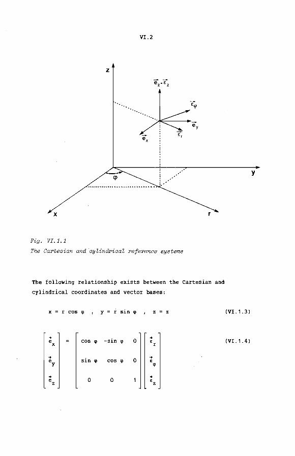
VI.2
z
x
Fig. VI.l.l
The Cartesian and cylindrical reference systems
The following relationship exists between the Cartesian and
cylindrical coordinates and vector bases:
x = r cos lP y i: sin q> z = z
... -sin 0
.. e cos (j) (j) E x r
.. sin 0
.. e (j) cos (j) E
y (j)
.. e 0 0
.. E z z
y
(VI .1. 3)
(VI.1.4)

VI. 3
Every CRS point is identified unambiguously by a set of CRS coor
dinates g. Moreover, every CRS point can be identified by means of
the Cartesian and cylindrical coordinates of that point in a state t.
In section VI.2 an axisymmetric element is presented which is used
for the simulation of the forming process . Various relevant
quantities at a point of this element are considered. Veetors and
tensors are written in components with respect to the cylindrical
basis at that point. For a vector ~ we write
.. a
T .. a E
..T E a
where column a contains the cylindrical components of ~.
(VI.1.5)
The state in which the geometry of an element is optimal, is called
tf. In this state, the fictitious material associated with the
element is stress-free . In state t, the Cauchy stress tensor at a
point of the element, the value of which depends on the deformation
of the fictitious material at this point with respect to state tf' is
a measure for the deviation from the optimum geometry of the element.
Rigid body movement of the fictitious material must not affect these
stresses. For this reason the axisymmetric element is not appropriate
for simulating the CRS determination process . The fictitious material
is considered to be associated with a plain-strain element which is
introduced in section
sidered
written
point .
.. a
at a point of
in components .. For a vector a
T .. a e
.. T e a
VI.3. Various relevant quantities are con-
this element. Veetors and tensors are being
with respect to the Cartesian basis at that
we write
(VI.1 . 6)
where column a contains the Cartesian components of ~ .
Some detailed aspects of the CRS determination process are discussed
insection VI . 4.

VI.4
VI.2 An axisymmetric element
The axisymmetric element, used to siaulate the forming process, is
shown in figure VI.2.1.
z
x
Fig. VI. 2.1
The axisymmetrio element
The cross~section is a quadrilateral with straight sides . For the
local CRS coordinates we find
y
(VI.2.1)
Each
that
local coordinate lies within the interval [-1,1]. It is assumed
~ = v for every ~ with 0 < ~ i 2v. 3g2
None of the relevant quantities in an axisymmetric forming process is
a function of the ~- or g2-coordinates. Thus attention can be fixed
on one cross- section of the element, e.g. with ~ = 0. The bilinear

VI. 5
interpolation functions used, are merely a function of the local CRS
coordinates g1 and g3. The four vertices of the quadrilateral cross
sectien are the nodal points used for the interpolation. The four
interpolation functions are contained in the column ~:
~ ~1 1 4( 1-g1 )( 1-g3) (VI.2.2)
1112 1 4 ( 1+g1 )( 1-g3)
"'3 1 4( 1+g1) ( 1+g3)
"'4 1 4( 1-g1 )( 1+g3)
A scalar quantity a at a point of the element is interpolated as
follows
1 a
2 a 3
a 4
a
(VI.2.3)
where column a contains the values of a at the element nodal points.
A vector ~ is interpolated as
If
to
.. T .. a Ijl a
the nodal point
the cylindrical
.. veetors a are
vector basis,
.. T T .. [ljl1 "'2 "'3 ljl4) a Ijl a E = a
a
a
a
(VI.2.4)
written into components with respect
we can write
1 1 1 .. a a E (VI.2.5) r lil z r
2 2 2 .. a a E r lil z lil
3 3 3 .. a a e: r lil z z
4 4 4 a a r lil z
VI.6
According tó (!! . 2 . 61) the CRS vector basis ~at CRS point q of the
element is defined by
~ .. .. VT [_a _ __Q_ _i_ J (VI.2.6) V X V p
~q ~q ~q ag1 ag2 agJ
.. Here p is the position ,vector of point g. In components with respect
to the Cartesian vector basis .. e in q we can write
.. T .. [x z]
.. p P e y e x (VI.2. 7)
.. e y
.. e z
and hence
~ T .. .. Qx_ Qy_ 2..L (V p )e ~ e ~x ~9~ ~ -x~ ag1 ag1 ag1
(VI.2 . 8)
a x Qy_ 2..L ag2 ag2 ag2
.Q.L Qy_ 2..L agJ agJ ag3
With (VI.1.3), (VI.1.4) and (VI.2 . 1), ~ can be written in components .:;
with respect to the cylindrical basis t in g as
~ .. 2.L 2..L = f3 E ~c ag1
0 ag1
(VI.2.9) -c~
0 11r 0
ar 0 az agJ agJ
VI. 7
Interpolating the cylindrical coordinates r and z according to
(VI.2.3), the matrix ~c becomes
ilij?
.!!c -~- r ilg1 ~
0 (VI. 2. 10)
0 T 11\jl r 0
(llj,T - r ilg3 ~
0
The Jacobian J of the mapping .. x G -+ V(t) is defined by
(VI. 2 . 11)
If the basis veetors pi (i= 1,2,3) are written in components with
respect to the cylindrical basis ~. it is easily shown that
The redprocal
-+ -+T ll-'f I
It both p and
results in
-+ -+T T I! E.E 'f -c~ ~ - c
vector basis ..
can be determined from 'f
.. are written components with respect to 'f ~n
I
Because of the orthonormality of ~ we find for 'f -C
-T !c = ~c
(VI.2. 12)
(VI. 2. 13)
.. this EI
~
(VI. 2. 14)
(VI. 2. 15)
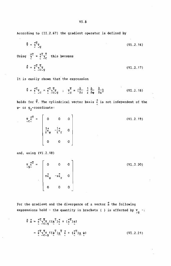
VI.8
According to (!!.2.67) the gradient operator is defined by
.. .. T V "Y V ' , g (VI.2.16)
Using '+T -+T T this becomes "Y = E :!c '
.. -+T -yTV V E
' -c,g (VI.2.17)
It is easily shown that the expression
.. V (VI.2.18)
holds for V. The cylindrical vector basis ; is not independent of the
~- or g2-coordinate :
-+T 0 0 0 V E ,c, (VI.2 . 19)
1 .. 1 .. 0 -E --E
I ~ I I
0 0 0
and , using (VI. 2. 18)
-+T 0 0 0 V E ,g, (VI. 2. 20)
.. .. 0 l!E - l!E
~ I
0 0 0
For the gradient and the divergence of a vector ~ the following
expressions hold - the quantity in brackets ( ) is affected by v ,g
(VI. 2 . 21)
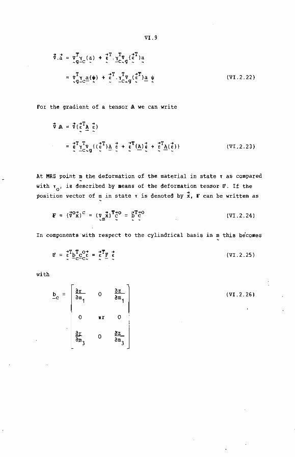
VI. 9
.. .. VT'Y (a) -+T T -+T
V.a + E .'( V (E )a ~g-e ~ -C~g ~
T -+T T -+T Ijl V 'Y a(ljl) + E .'( V (E )a
~g-e-:- ~ -C~g ~ (VI.2 . 22)
For the gradient of a tensor ~ we can write
(VI.2 . 23)
At MRS point m the deformation of the material in state 1 as compared
with 10
, is described by means of the deformation tensor F . If the
position vector of m in state 1 is denoted by ~. F can be written as
F -+T-+o b c (VI.2 . 24)
In components with respect to the cylindrical basis in m this bécomes
F -+T T o-+ ~TF .. E b C E E ~ -c-c~
(VI.2.25)
with
b .k_ 0
Q.L -C am1 am1
(VI.2 . 26)
0 11r 0
ar 0 2.L
am3 am3

VI.10
VI . J A plain-strain element
A plain-strain element is used to simulate the CRS determination
process, and is shown in figure VI.3.1.
z
x
Fig . VI . 3 . 1
The pZai n- strain e l ement
With every axisymmetric element a plain-strain element having the
same cross-section for ~ = 0 is associated. The local CRS
coordinates are such that
(VI . 3 . 1)
Each local coordinate lies within the interval [-1,1]. Moreover,
has an arbitrary but equal value a for all y .
In the plain-strain CRS determination process none of the relevant
quantities is a function of the y- or g2-coordinates. The inter
polation functions and nodal points used to interpolate these quan
tities are the same as those presented in section VI . 2 for the
axisymmetric element. For a vector ~ we write
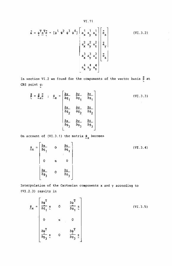
V!o11
.. T T .. [ljl1 ljl2 ljl3 ljl4] 1 1 1 .. (VI.3o2) a 111 a e a a a e x y z x
2 a2 2 .. a a e x y z y
3 3 3 .. a a a e x y z z
4 4 4 a a a x y z
Insection VI 02 we found for the components of the vector basis jl at
CRS point g:
p = jl ; ~x fuL .Q.y_ QL
~ -x~ élg1 élg1 élg1 (VI. 3 o 3)
fuL .Q.y_ QL élg2 élg2 élg2
k_ .Q.y_ QL élg3 élg3 élg3
On account of (VI. 3 0 1) the matrix P becomes -X
~x k_
0 QL
élg1 élg1 (VI.3o4)
0 Cl 0
k_ 0
QL élg3 élg3
Interpolation of the Cartesian components x and y according to
(VI.2.3) results in
élljlT él$T
!x ~x
élg 1 ~ 0 _.,_ z
élg 1 ~ (VI.3 o5)
0 Cl 0
él$T élljlT -~-x 0 - z élg3 ~ élg3 ~
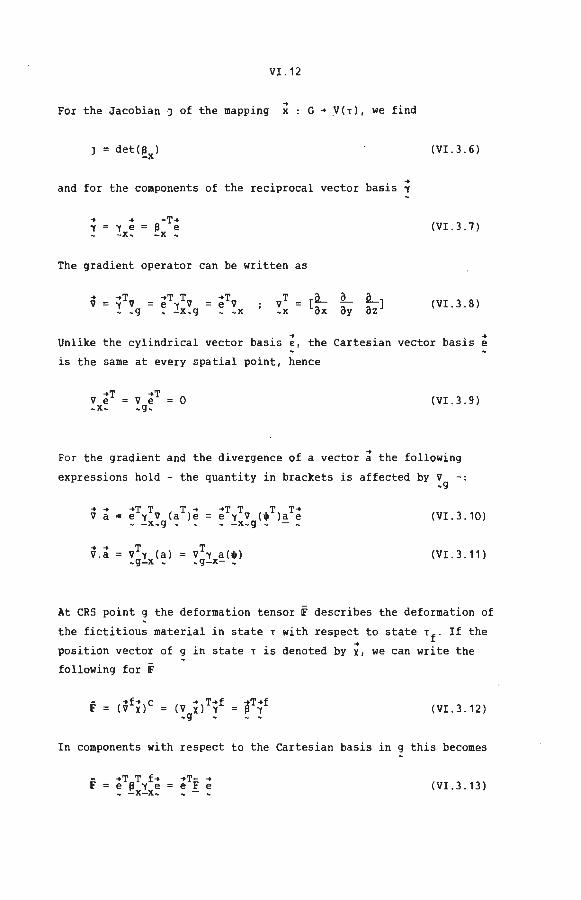
For the Jacobian J of the mapping
VI. 12
.. x G .. V(t), we find
J = det(~x) (VI.3.6)
and for the components of the reciprocal vector basis i
.. .. l l e
-X·
The gradient operator can be written as
.. V
.. T T e l V • -X.g
.. T e v •• x
(VI.3.7)
(VI. 3. 8)
Unlike the cylindrical vector basis ;, the Cartesian vector basis~
is the same at every spatial point, hence
V ~T 0 .g.
(VI. 3. 9)
For the gradient and the divergence of a vector ~ the following
expressions hold - the quantity in brackets is affected by V - : .g
.. .. V a (VI. 3. 10)
.. .. V.a (VI.3.11)
At CRS point g the deformation tensor F describes the deformation of
the fictitious material in state T with respect to state 'f· If the
position vector of g in state T is denoted by ~. we can write the
following for F
(VI.3.12)
In components with respect to the Cartesian basis in g this becomes
.. T T f .. e P l e • - x-x.
..T- .. e F e (VI. 3 . 13)
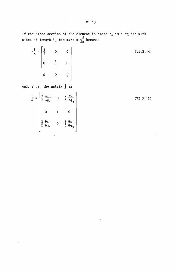
VI. 13
If the cross-section of the element in state Tf is a square with . fl 1 • fb s1des o ength & 1 the matr1x 1 · ecomes
-X
f 2 0 0 ::!x z (VI. 3 . 14 l
0 I
0 Cl
0 0 f z
and, thus , the matrix F is
F 2 ox
0 2 OX
ï og1
ï og3
(VI. 3. 15 l
0 0
2 oz 0 2 oz ï og
1 ï og3
VI .14
VI.4 Aspects of the CRS determination process
The optimum element geometry
The coupZing between CRS and MRS
The optimum e lement geometry
The axisymmetric element used to simulate the forming process is
presented in section VI.2. The shape of its cross-section may affect
the accuracy of the numerical integrations and the error, possibly
introduced by the interpolation of the MRS displacement à x . We m e assume the accuracy of the numerical integration to be maximal and
the error caused by interpolation to be minimal if the cross-section
is a square . This shape is called the optimum shape.
Both the size and the shape of the cross-section may affect the
interpolation error. In view of the size the error can be assumed to
be minima!, if the area of the cross-section is a given function of
the stress gradient within and in the neighbourhood of the element.
Various ideas have been published in literature as to the optimum
size of elements (see Turcke & McNeice (1974), Melosh & Marcal
(1977), Chiou & Wang (1979), Babuska & Rheinboldt (1979, 1980), Dwyer
et al. (1980), Zienkiewicz et al. (1981, (29]) and Bathe & Sussman
(1983)). In the CRS determination process discussed in this thesis
the optimum size of elements is not considered .
The length in y-direction of the plain-strain element in state Tf is .. f
so chosen that the reciprocal vector basis 1 at every CRS point is
(VI. 4. 1)
In the current state T the deformation tensor at CRS point g, which
describes the deformation of the fictitious material at that point
compared to state Tf' is denoted by ~f (see figure VI.4 . 1) .
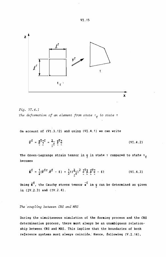
z
Fig. VI. 4.1
"( ' f
VI .15
The deformation of an element from state Tf to state T
On account of (VI.3.12) and using (VI.4.1) we can write
-f ;tT .. f IF = I' "'f
x
(VI. 4. 2)
The Green-Lagrange strain tensor in g in state T compared to state Tf
becomes
-1 { ( 2.....) 2 .. T .... T .. e ~-~ e - [) 2 lf
(VI. 4. 3)
Using Ëf, the Cauchy stress tensor ;f in g can be determined as given
in (IV.2.3) and (IV.2.4).
The coupZing between CRS and MRS
During the simultaneous simulation of the forming process and the CRS
determination process, there must always be an unambiguous relation
ship between CRS· and MRS. This implies that the boundaries of both
reference systems must always coincide.· Hence, following (V.2.14),
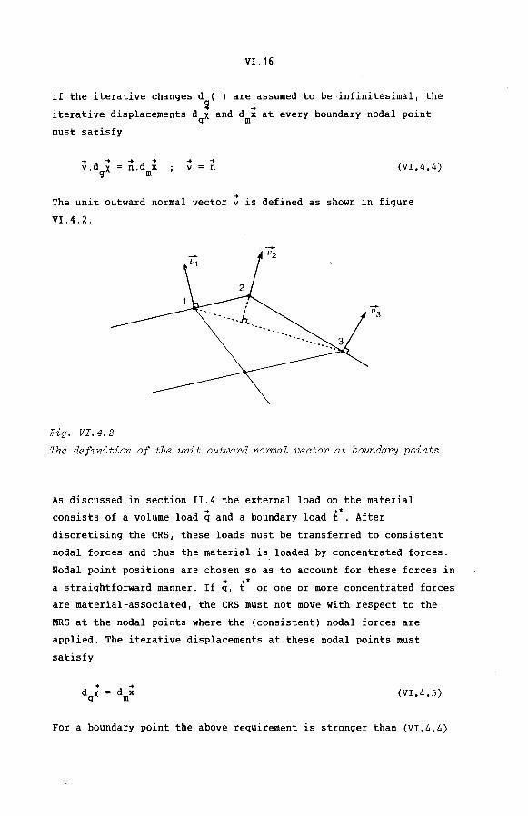
VI .16
if the iterative changes d ( ) are assumed to be infinitesimal, the • . . ~ -+ 1 . 1terat1ve d1splacements d x and d x at every boundary noda po1nt
g m must satisfy
-+ V
-+ n (VI.4.4)
The unit outward normal vector ; is defined as shown in figure
VI. 4. 2.
Fig. VI.4.2
The definition of the unit outwaPd nonmal veetoP at boundapY points
As discussed in section II.4 the external load on the material -+ -+*
consists of a volume load q and a boundary load t . After
discretising the CRS, these loads must be transferred to consistent
nodal farces and thus the material is loaded by concentrated farces.
Nodal point positions are chosen so as to account for these farces in -+ -+*
a straightforward manner. If q, t or one or more concentrated farces
are material-associated, the CRS must not move with respect to the
MRS at the nodal points where the (consistent) nodal farces are
applied. The iterative displacements at these nodal points must
satisfy
(VI.4.5)
For a boundary point the above requirement is stronger than (VI.4,4)

VII.1
VII Simulation of axisymmetric forming processes
. 1 Introduetion
. 2 A simulation program
. 3 Results of some simulations
VII.1 Introduetion
A computer program is developed to test the method described in the
preceding chapters . With this program numerical simulation of axi
symmetric forming processes can be carried out, using either the
Lagrangian or the AEL formulation. It is also possible to employ the
rezoning technique . The program is written in Burroughs Extended
Algol and implemented on the Burroughs B7700 computer of the
Eindhoven University of Technology. Some program items concerning the
simulation according to the AEL formulation are discussed in section
VII.2. Results of some simulations are presented in section VII.3.
VII.2
VII.2 A simulation program
For the simulation of a forming process according to the AEL tor
mulation the following sequence of instructions is carried out by the
program.
1: define initial model;
while increments-to-calculate do
begin
2 : define new increment;
while no-convergence do
begin
3 :
4:
5 :
6:
7 :
8:
9:
10:
11 :
12 :
13:
calculate CRS nodal point forces ;
make system of equations;
introduce kinematic boundary conditions and coupling
conditions for CRS and MRS;
calculate iterative CRS and MRS displacements at nodal
points;
adjust CRS nodal point displacements;
calculate material-associated quantities at follower
points;
update geometry and location;
update material-associated data at follower points;
transfer material-associated data from follower points to
integration and nodal points;
calculate residual nodal point forces ;
check convergence;
end;
end.
These instructions will be discussed shortly.
1: Data on geometry, connectivity, kinematic and dynamic boundary
conditions and material behaviour are input data for the
program. It is possible to interrupt the simulation and restart
with the same or partly changed boundary conditions. In that
case, the data on the deformation history must also be available
as input data.
VII. 3
2: At the beginning of every increment the follower points are
redefined, to be the MRS points, coinciding with the nodal
points and the mid-points of element sides and elements .
Defining the follower points determines the cells as well. For
every nodal and integration point are stipulated the cell in
which it is situated and its local MRS coordinates within this
cell . Material-associated data at the nodal points are
transferred to the new follower points by interpolation .
3 : The nodal forces arising out of the deviation of optimum element
shape, are determined according to the method described in
chapter IV and section V. 4 .
4 : The iterative CRS and MRS displacements d x and d ~ must satisfy g, m, the systems of linearised equations (V . 2 . 13)
I d ~ m,
d .. g~
= (VII.2.1)
If the material is (nearly) incompressible, as is the case in
some elasto-plastic forming processes, the axisymmetric element
used, may behave much too stiffly, as is described by Nagtegaal
et al . (1974) and Nagtegaal & De Jong (1981). To prevent this
"locking", reduced numerical integration is employed for those
termsin (VII . 2 . 1), which characterize the hydrastatic material
behaviour.
5: At a nodal point the two components of d x and d ~are either g m suppressed, prescribed (nonzero) or unknown . At a boundary point
we want to satisfy the coupling condition (V .2 . 14), that is
where -+i V
(VII.2 . 2)
-+i 0 0
n ~s the un~t outward normal vector at that point.
At some points the coupling condition (VI.4.5) has to be
satisfied, that is
.. d x g
VII .4
d ~ m (VII. 2. 3)
Satisfying (VII.2.2) or (VII.2.3) means coupling one or both
components of d x and d ~- The coupled components are denoted by g m
an index c, the free but unknown components are denoted by an
index Ü (ford x) and u (ford~). After dealing with the sup-g m
pressed and prescribed components in the usual way, the system
of equations (VII .2 .1) can be written as follows
A A B - B d x ~1u (VII.2.4) -u u -uc -u u -uc m.u A A B - B d x ~1c -CU -cc -CU -cc m.c 0 0 V-- V- d g~Ü R -
-UU -UC .2u 0 0 V - V d g~c ~2c -CU -CC
Taking d x = d x into account and deleting the equations with g.c m.c the unknown right-hand vector R
2 leaves us with
- c
[
A A -UU -UC A A -cu -cc 0
+ B -UC
+ B -cc
v-ue
B -1 [d x 1 -uu m.u B - d x -cu m.c v-- d x-uu g.u [
;1u1 .1c R -.2u
(VII.2.5)
6: The iterative displacement components d x , d x and d x- are m.u m.c g.u solved from (VII.2.5).
7: If the CRS and MRS boundaries coincide at the beginning of an
iterative calculation, they will still approximately
coincide after the iterative calculation, if (VII.2.2) is
satisfied and if the iterative displacements d x and d ~ are g m
infinitesimal. Since these displacements are finite the
boundaries will move apart, as is shown in figure VII.2.1 for
one nodal point.
To ensure that the CRS and MRS boundaries coincide as closely as
possible at the end of the iterative calculation, the itPrative
boundary riodal point displacements d x are adjusted: This is g
done in such a way that every boundary nodal point will finally
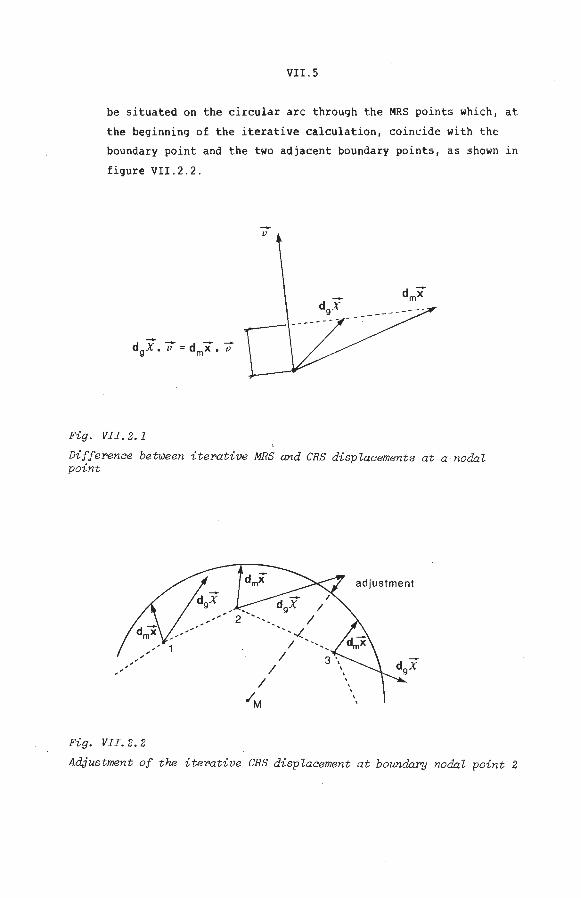
VII. 5
be situated on the circular are through the MRS points which, at
the beginning of the iterative calculation, coincide with thc
boundary point and the two adjacent boundary points, as shown in
figure VII. 2. 2.
V
Fig. VII. 2. 1
Difference between iterative MRS and CRS displacements at a nodal point
adjustment
Fig. VII. 2. 2
AdJustment of the iterative CRS displacement at boundary nodal point 2
VII. 6
B: The material-associated quantities are determined at the fol
lower points. After calculating the iterative change of the
deformation tensor F, according to
d F m
(VII.2.6)
the iterative change of the Green-Lagrange strain tensor is
calculated in accordance with
d IE m
(VII . 2 . 7)
The Cauchy stress tensor and the current yield stress are deter
mined according to the procedure described in section V.4 . The
hardening parameter is constant in value, as the hardening is
supposed to be linear.
9: Calculating the new position of the nodal points is very
straightforward. For every follower point it is determined in
which element this point is situated and what its local CRS
coordinates are within this element. The same applies, for every
nodal point, to the cell in which this point is situated and
what its local MRS coordinates are within this cell .
Although the iterative boundary nodal point displacements are
adjusted , the CRS and MRS bouridaries will not coincide exactly
as is shown in figure VII . 2.3 . This deviation is unavoidable and
in most cases very slight . However, follower points may fall
outside the element mesh. This must be corrected for two
reasons, the first being that one or m.ore cells will not then be
defined . Second, material-associated data must not be lost to
the new .element mesh. For every follower point, situated outside
the element mesh, a new follower point is defined as shown in
figure VII.2.4 .
10: The material-associated data at the new follower points are
calculated by interpolation between the data at points ~ 1 and
~z·

VII. 7
Fig . VII. 2. J
Deviation of the CRS and MRS boundaries
Fig. VII . 2. 4
I I
--. ~ ~-
'.!1,
Definition of a new fo llower point
' ' ' '
' ' ' ' ' ·
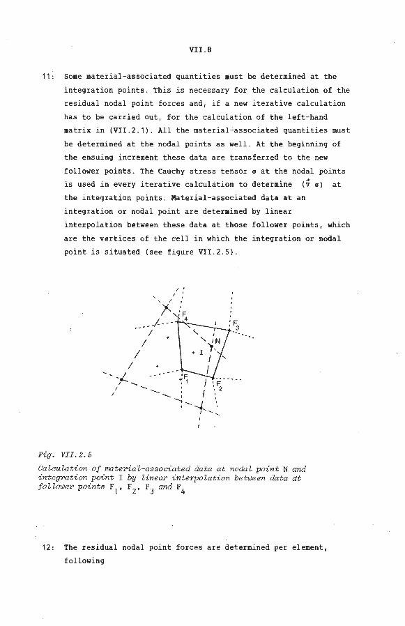
VII.S
11: Some material-associated quantities must be determined at the
integration points. This is necessary for the calculation of the
residual nodal point farces and, if a new iterative calculation
has to be carried out, for the calculation of the left-hand
matrix in (VII.2.1) . All the material-associated quantities must
be determined at the nodal points as well. At the beginning of
the ensuing increment these data are transferred to the new
follower points. The Cauchy stress tensor m at the nodal points
is used in every iterative calculation to determine ..
(V m) at
the integration points . Material-associated data at an
integration or nodal point are determined by linear
interpolation between these data at those follower points, which
are the vertices of the cell in which the integration or nodal
point is situated (see figure VII.2.5).
Fig. VII . 2. 5
I • I :
' I '
!'- -J F _ __ _ /- --- 4
I I
I I
-' -i I --I
I
Ca lculat ion of mat erial- associated da t a at nodal poin t N and i ntegPat ion point I by l i neaP i ntePpolati on between data at followeP points F
1, F
2, F
3 and F
4
12: The residual nodal point farces are determined per element,
following
VII. 9
Ri .. i ... •i • J Ijl qeJe dG + r. Ijl t eJe dG
~1e G G e e
J ( ljJT)T .. i i i dG - V "Y . GJ J G ~9~ ~e e e
(VII.2.8)
e
.. ... Volume loads q and surface loads t are taken into account by
.. k concentrated nodal point forces r which are applied aftcr
assembling the elements. The total residual nodal force vector
then becomes
(VII.2 . 9)
When the iterative calculation is terminated, the equivalent
nodal force vector ~ 1 , defined by
.. ~1
n [ f
e=1 G e
T T .. (V Ijl ) "Y . GJ J dG ~9~ ~e e e (VII.2 . 10)
is taken into account in the first iteration step of the next
increment, by adding it to the new external nodal force vector.
13 : The accuracy of the current approximated solution for the
incremental MRS displacement
accuracy is a norm of d ~ or m~
à ~. is checked . A m~
~ 1 . If the "exact''
measure for this
salution for ll ~ m~
is obtained, these norms are both zero. The approximation is
considered to be accurate enough if one of these norms is
smaller than an associated limit value. In that case the
iteration process is converged and a new incremental calcul ation
can be started.
VII. 10
If the Lagrangian formulation is used in the numerical simulation,
the iterative nodal point displacements have to satisfy th~ system of
linearised equations given below, resulting from (VII . 2 . 1) with
d ~ = d ~. that is g~ m~
i i ~ (IA +!! ).dm~
.. i ~1 (VII. 2. 11)
The integration points act as follower points. The program steps 2,
3, 7, 10 and 11 are dropped completely, whereas others are carried
out partly .
If the rezoning technique is employed in the simulation, the
iterative displacements d x and d i are calculated in two steps . 9~ m~ •
First .the iterative nodal point displacements d x are determined so 9~
as to satisfy the system of linearised equations
("VII . 2 . 12)
obtained from (VII . 2.1) with di= 0. After defining the new element m~
mesh resulting from these iterative nodal point displacements,
material-associated data are transferred from follower points to
integration points by interpolation as already described.
In the secend step the simulation is continued using the new element
mesh and the Lagrangian formu~ation . The nodal point displacements
d ~are determined so as to sà,tis fy (VII.2.11) . The total iterative m~ ,
nodal point displacements are
(VII.2 . 13)
The material-associated quantitles are determined at the follower
points. Finally these data are transferred to integration and nodal
points in the usual way.

VII . 11
VII.3 Results of some simulations
The first process which is analysed, clearly shows the possibilities
of the AEL formulation . We consider the circular disk, shown in
figure VII . 3.1. In five equal incremental steps the radial
displacement of the outer edge is prescribed. The ultimate radial
strain is 25\. The dashed area is considered in the simulation .
Fig. VII . 3. 1
CiPculaP disk: geometPy and material paPametePs
E = 2.1 • 105
N /mm2
V = 0.3 h = 10
4 N/mm2
o~ = 250 N/mm2
E = 100 N/mm2
îi = 0.45 measures in mm
If the material behaviour is elasto-plastic the analytica! solution
for the stress components is given by
0 rr 0 qup
0 = 0 zz
o 2Eh 1 ov + E + 2h(1 - v) . l~ln(1 + 2Err) -
(VII.3 . 1)

VII. 12
The use of the Lagrangian tormulation leads to the result shown in
figure VII.3 . 2a. Using the AEL tormulation leads to the result which
is shown in figure VII . 3 .2b.
a
Fig. VII.3. 2
lli:J frf1 F1 !Hl t I I! I I l I I I I I I I I I I I I I.
b
Element mesh i n vaPious states of t he defo~ation process, using the Lagrangian (a) and the AEL (b) formulation
As we can see all elements have the same geometry in the final state
if the AEL tormulation is used. Using the rezoning technique also
leads to the result shown in figure VII . 3 .2b . In all cases and every
increment, convergence was reached after the same number of iterative

VII. 13
calculations and then the stresses had the exact values given by
(VII . 3 . 1) .· The ratio of the total process time was (in seconds)
Lagrangian rezoning AEL 137 195 207 (VII. 3. 2)
The use of the AEL tormulation provides the possibility to suppress
or prescribe nodal point displacements or nodal point forces in a
straightforward manner, while at the same time the material
displacement at these points is an unknown quantity, which can be
determined. In figure VII . 3 . 3 the undeformed (dotted) and the
deformed state of the circular disk is shown both when the Lagrangian
tormulation (a) and the AEL tormulation (b) is used . Using the AEL
tormulation the following conditions are chosen
0
.. d x
m
r- ... ,.. • .. , ..... -.-- .. ··.- ... • .,
Hl+t·tt:··--t! I a
Fig. VII. 3. 3
at points 1-9 (VII . 3.3a)
at all other points (VII . 3 . 3b)
r- ., .. - -,. ... ··- ... .._ .... - .. • t I I t t f
: ' ' : 3
2
b
Element mesh in undefoY'ITied and defoY'ITied state, using t he Lagrangian (a) and the AEL (b) formuZation
The following simulation is carried out merely to show the pos
sibility o.f optimizing element geometries, even if all nodal points
are situated on a curved boundary. We consider the body and initial
element mesh, shown in figure VII.3.4.
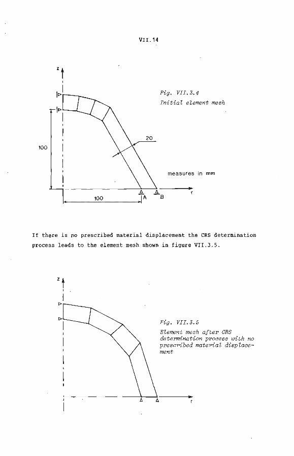
VII . 14
Fig. VII.3.4
Initial element mesh
100
measures in mm
100
If there is no prescribed material displacement the CRS determination
process leads to the element mesh shown in figure VII.3 .5.
Fig. VII. 3. 5
Element mesh after CRS de termination process with no prescribed material disp lacement
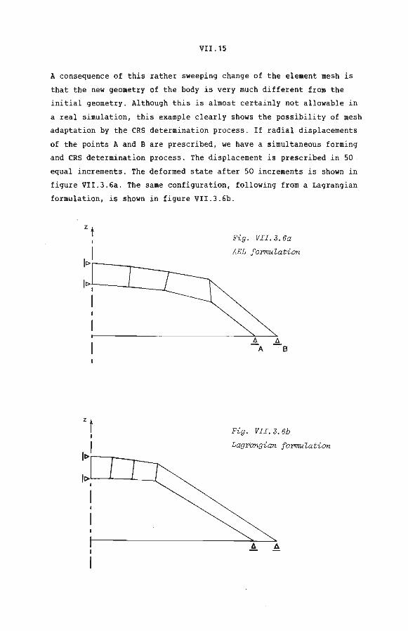
VII. 15
A consequence of this rather sweeping change of the element mesh is
that the new geometry of the body is very much different from the
initia! geometry . Although this is almast certainly not allowable in
a real simulation, this example clearly shows the possibility of mesh
adaptation by the CRS determination process. If radial displacements
of the points A and B are prescribed, we have a simultaneous forming
and CRS determination process . The displacement is prescribed in 50
equal increments . The deformed state after 50 increments is shown in
figure VII . 3.6a . The same configuration, following from a Lagrangian
formulation, is shown in figure VII.3.6b .
lt>;--, ---L __ _j
I
Fig . VII. 3. 6a
AEL fo mru Zation
Fig . VII . 3. 6b
Lagrangian f omruZation
A
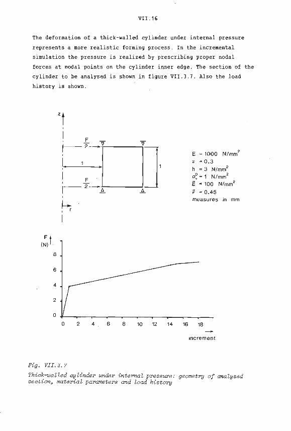
VII. 16
The deformation of a thick-walled cylinder under internal pressure
represents a more realistic forming process . In the incremental
simulation the pressure is realized by prescrihing proper nodal
forces at nodal points on the cylinder inner edge. The section of the
cylinder to be analysedis shown in figure VII.3.7 . Also the load
history is shown .
I F -- V V
!-2--.r---;]1 I F I r-2--1::.~-----'1::. '
~ I
I
8
6
4
2
0
0 2 4 6 8 10 12 Fig. VII. J. 7
14 16
E = 1000 N/mm2
V = 0.3
h = 3 N/mm2
o~ = 1 N/mm2
E = 100 N/mm2
ïi = 0.45
measures in mm
18
iocrement
Thick-walled cylinder under internal pressure : geometry of analysed section, material parameters and laad history
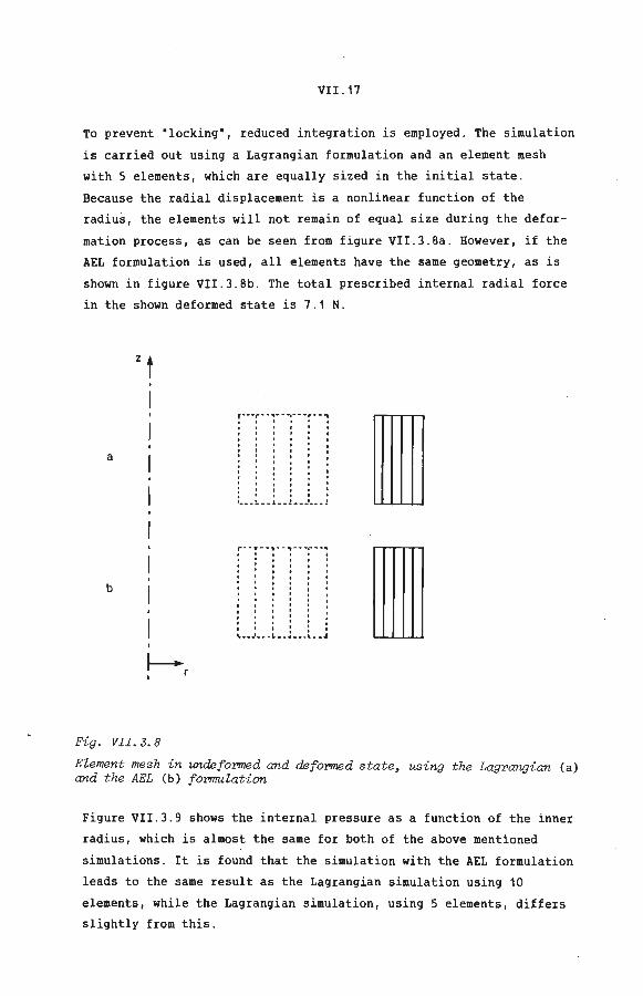
VII. 17
To prevent "locking•, reduced integration is employed. The simulation
is carried out using a Lagrangian tormulation and an element mesh
with 5 elements, which are equally sized in the initia! state .
Because the radial displacement is a nonlinear function of the
radius, the elements will not remain of equal size during the defor
mation process, as can be seen from figure VII . J.Ba. However, if the
AEL formulation is used, all elements have the same geometry, as is
shown in figure VII . J . Bb. The t otal prescribed internal radial force
in the shown deformed state is 7 .1 N.
a
b
t--r •
Fig . VII. 3. 8
r··•r• ... ,. .. . ..,---r· .. ., 4 ~ t I I I 0 0 0 0 0
• 0 •
• ...... L .... 1 .... .! ..... .' .. ~ .. .:
r- -.--, · --. -- -~"""'""''"'
0
• • I I 0
: : ; : : : .... ........... L .... ~-- -"' - -.1
Element mesh in undefor'ITied and de f or'ITied state , using the Lagrangian (a) and the AEL (b) for'ITIUlation
Figure VII . 3.9 shows the internal pressure as a function of the inner
radius, which is almost the same for both of the above mentioned
simulations . It is found that the simulation with the AEL formulation
leads to the same result as the Lagrangian simulation us ing 10
elements , while the Lagrangian simulat i on, usi ng 5 element s, differ s
slightly from this.
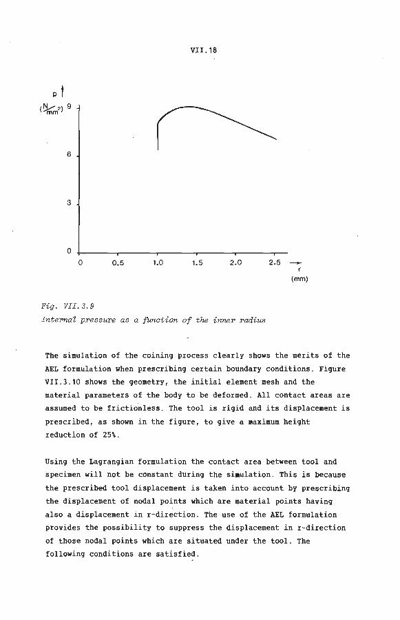
VII .18
0 0.5 1.0 1.5 2.0 2.5 -
(mm)
Fig . VII. 3. 9
Internar pressure as a funetion of the inner radius
The simulation of the coining process clearly shows the merits of the
AEL formulation when prescrihing certain boundary conditions. Figure
VII.3.10 shows the geometry, the initial elementmeshand the
material parameters of the body to be deformed. All contact areas are
assumed to be frictionless. The tool is rigid and its displacement is
prescribed, as shown in the figure, to give a maximum height
reduction of 25\.
Using the Lagrangian formulation the contact area between tool and
specimen will not be constant during the simulation. This is because
the prescribed tool displacement is taken into account by prescrihing
the displacement of nodal points which are material points having
also a displacement in r-direction. The use of the AEL formulation
provides the possibility to suppress the displacement in r-direction
of those nodal points which are situated under the tool . The
following conditions are satisfied.

VII. 19
0 for 0 i r 0 i 9
(VII.3 . 4)
for 9 < r 0 i 18
The deformed geometry is shown in figure VII . 3.11a. The same
simulation is carried out with more nodal point displacements
suppressed in r-direction , according to the conditions
0 for 0 i r 0 i 13.5
(VII. 3. 5)
d ~ m
for 13 . 5 < r 0 i 18
The deformed geometry is shown in figure VII.3 . 11b. The stress
component azz in the contact area between tool and specimen for both
the conditions (VII . 3 . 4) and (VII.3 . 5) is shown in figure VII . 3. 12.
It is obvious that the simulation according to (VII . 3 . 5) leads toa
more realistic deformation and that the tool-specimen stress is
smoother.
Fig. VII. 3. 10
E • 2.1·105
N/mm2
v • 0.3 h • 10
4 N/ mm
2
o0• 250 N/mm
2 V
measures in mm
Geometry, initial element mesh and material parameters for the coining process
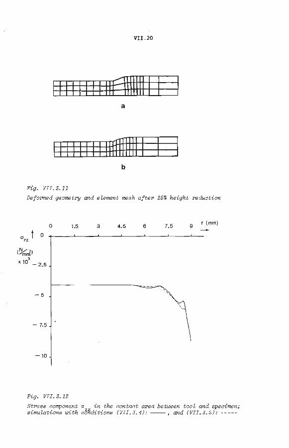
VII. 20
1111111111Alllllll I a
111111111 mfflllll I b
Fig. VII. 3. 11
Deformed geometry and element mesh after 25% height redu~tion
0 1.5 3 4.5 6 7.5 9 r (mm)
(~2) mm 3
x 10 -2.5
-5
-7.5
-10
Fig. VII. 3.12
Stress component a in the contact area be tween tool and specimen; sirrrulations with cB'fiditions (VII.3 .4) : --, and (VII . 3.5): --- --
VIII. I
VIII Concluding remarks
If the finite element method and the Lagrangian tormulation is used
to simulate forming processes, the elements are associated with the
material. Large local deformations may cause excessively distorted
elements which may give rize to numerical difficulties . To prevent
this problem a number of ad hoc solutions is known, such as the
rezoning technique, where, if necessary, the simulation is
interrupted and restarted with a new element mesh .
This thesis describes the results of research on the application of
the Arbitrary-Eulerian-Lagrangian (AELJ tormulation for the
simulation of forming processes. Using this tormulation the element
mesh is not associated with the material to be deformed . However, it
is necessary that there is an unambiguous relationship between the
points of elementmeshand material. The theoretica! background of
the AEL tormulation is presented and some new conceptions are
introduced. In the mathematica! formulations a vector-tensor notation
is used.
The flexibility, provided by the AEL tormulation concerning the
choice of the element mesh, can be used to optimize the shape of
individual elements. The optimization described in this thesis is a
continuous and automatic process. The position and geometry of the
elements result from the deformation of a fictitious, isotropic,
elastic material - Young's modulus Ë, Poisson's ratio ~ -, which is
associated with the element mesh.
The methad is applied to the simulation of axisymmetric forming
processes. Theelastic material behaviour is isotropie and linear,
while isotropie hardening is assumed in the elasto-plastic range.
The automatic optimization of the element shape leads to good results
for the simulation of the considered forming processes. It appears
that the Young's modulus E does not affect the optimization, whereas
this is less apparent if a higher value of ~ (0 i~ < 0.5) is chosen .
The AEL tormulation is very appropriate not only to generate a
suitable element mesh but also to take certain boundary conditions
into account.
VIII. 2 .
As the element mesh is not associated with the material to be
deformed, materi~l-associated quantities are calculated at follower
points, being material points, which are redefined several times
during the simulation. Subsequently the material-associated data are
transferred to the integration points by interpolation. This provokes
inaccuracies, which disturb the nodal point equilibrium, causing the
convergence rate of the iterative procedure to decrease.
Because of thc fact that, besides the forming process, the
deformation of the fictitious material is considered and because of
the necessary use of follower points, a relatively large amount of
data in the analysis occurs. Moreover, the computer time needed for
an analysis is rather long. This is partly caused by the low
efficiency of the program, which aspect did not receive to much
attention.
Resuming we can concludc that the use of the AEL formulation and the
finite element method to simulate forming processes is very
advantageous for automatically optimizing element shape and
accounting for certain boundary conditions. The merits of the
formuiation will increase if further investigation is done concerning
the possibilities of the presented method.
It is possible to adapt the element size to, for instance, the stress
gradient within and in the neighbourhood of an element. For a real
optimization of the element mesh it will generally be also necessary
to adapt the number of elements . Further research on automatic
optimization of element size and number of elements is required.
Combining the AEL formulation with the use of gap-elements offers the
possibility to simulate processes where contact phenomena occur, even
if the contact surfaces show large relative displacements. Further
theoretica! investigation of the contact phenomena and the coupling
between the boundaries of the element mesh and the material is
necessary.
It is recommendable to explore possibilities to adapt the presented
method in such a way that the convergence rate of the iterative

VIII.3
procedure increases. Also, attention must be given to improve the
efficiency of the program.
IX. 1
IX Referenc~s
Babu!lka I., Rheinboldt W.C. (1979)
Adaptive approaches and reliability estimations in finite
element analysis. Computer methods in applied mechanics and
engineering, Vol. 17/18, pp. 519-540.
2 Babu!lka I., Rheinboldt W.C. (1980)
Reliable error estimation and mesh adaptation for the finite
element method. Computational methods in nonlinear mechanics
(ed. J.T. Oden), North-Holland Publishing Company, pp. 67-108.
3 Bathe K.-J., Sussman T.D. (1983)
An algorithm for the construction of optimal finite element
meshes in linear elasticity. Recent developments in computing
methods for nonlinear solid and structure mechanics, ASME
meeting, Houston, Ta., USA, june.
4 Belytschko T.B., Kennedy J.M. (1978)
Computer models for subassembly si~;.lation. Nuclear engineering
and design, Vol. 49, pp. 17-38.
5 Brekelmans W.A.M. (1982)
Over het integreren van de elasto-plastische constitutieve
vergelijkingen voor een drie-dimensionale spanningstoestand
bij Von Mises vloeicriterium, isotrope versteviging en geen
befnvloeding door de temperatuur. Personal notes.
6 Chiou S.-I., Wang C.-C. (1979)
Error estimates of finite element approximations for problems
in linear elasticity; part 1: Problems in elastostatics.
Archive for rational mechanics and analysis, Vol. 72,
pp. 41-60.
7 Donea J. (1978)
Finite element analysis of transient dynamic fluid-structure
interaction. Advanced structural dynamics (course), Commission
of the European Communities joint research centre, Ispra,
Italy, oktober.
IX.2
8 Donea J., Giuliani S., Halleux J.P. (1982)
An Arbitrary Lagrangian-Eulerian finite element method for
transient dynamic fluid-structure interactions. Computer
methods in applied mechanics and engineering, Vol. 33,
pp. 689-723.
9 Dwyer H.A., Kee R.J., Sanders B.R. (1980)
Adaptive grid method for problems in fluid mechanics and heat
transfer. AIAA journal, Vol. 18, pp. 1205-1212.
JO Gelten C.J.M., De Jong J.E. (1981)
A method to redefine a finite element mesh and its application
to metal forming and crack growth analysis. European conference
on nonlinear finite element analysis, The Hague,
The Netherlands, november.
IJ Hirt C.W., Amsden A.A., Cook J.L. (1974)
An Arbitrary Lagrangian-Eulerian computing method for all flow
speeds. Journal of computational physics, Vol. 14, pp. 227-253.
12 Huetink J. (1981)
Analysis of metal forming processes based on a combined
Eulerian-Lagrangian finite element formulation. European con
ference on nonlinear finite element analysis, The Hague,
The Netherlands, november.
13 Rughes T.J.R., Liu W.K., Zimmermann T.K. (1981)
Lagrangian-Eulerian finite element formu lation for incom
pressible viscous flows. Computer methods in applied mechanics
and engineering, Vol. 29, pp. 329-349.
14 Hutchinson J.W. (1973)
Finite strain analysis of elastic-plastic solids and structures .
Numerical solution of nonlinear structural problems
(ed. R.F. Hartung), ASME, N.Y., USA, Vol. 17, pp. 17-29.
IS Kennedy J.M., Belytschko T.B. (1981)
Theory and application of a finite element method for Arbitrary
Lagrangian-Eulerian fluids and structures . Nuclear engineering
and design, Vol. 68, pp. 129- 146.
IX.3
16 Krieg R.D., Krieg D.B. (1977)
Aaauraaies of numeriaal solution methods for the elastia
perfeatly plastic model. Journal of pressure vessel technology,
PP· 510-515.
17 Lai W.H., Rubin D., Krempl E. (1978)
Introduetion to continuurn meahanias. 4th. Edition (1979),
Pergamon Press.
18 Melosh R.J., Marcal P.V. (1977)
An energy basis for mesh refinement of struatural continua.
International journal for numerical methods in engineering,
Vol. 17, pp. 1083-1091.
19 Nagtegaal J.C., Parks D.H., Rice J.R. (1974)
On numeriaally accurate finite element solutions in the fully
pZastia range. Computer methods in applied mechanics and
engineering, Vol. 4, pp. 153-177.
20 Nagtegaal J.C., De Jong J.E. (1980)
Some aomputational aspeats of elastia-plastia large strain
analysis. Computational methods in nonlinear mechanics
(ed. J.T. Oden), North-Holland Publishing Company, pp. 303-339.
21 Nagtegaal J.C., Veldpaus F.E.
On the implementation of finite strain plastiaity equations
in a numeriaal model. To be published.
22 Pracht W.E. (1~75)
Calaulating three-dimensional fZuid fZows at aZZ speeds with
an Eulerian-Lagrangian aomputing mesh. Journal of computational
physics, Vol. 17, pp. 132-159.
23 Roll K., Neitzert T. (1982)
On the appliaation of different numeriaal methods to aalaulate
aold forming proaesses. Numerical methods in industrial forming
processes, Swansea, U.K., june.
24 Schoofs A.J.G., Van Beukering L.H.T.M., Sluiter M.L.C. (1979)
A general purpose two-dimensional mesh generator. Advances in
engineering software, Vol. I, pp. 131-136.

IX.4
25 Stein L. R., Gentry R.A., Hirt C. W. ( 1977)
Computational simulation of transient blast loading on three
dimensional structures. Computer methods in applied mechanics
and engineering, Vol. 11, pp. 57-74.
26 Turcke D.J., McNeice G.M. (1974)
Guidelines for selecting finite element grids based on an
optimization study. Computers and structures, Vol. 4,
pp. 499-519.
27 Zienkiewicz 0. C. ( 1977)
The finite element method. 3rd. Edition (1977), McGraw Hill
Book Company.
28 Zienkiewicz O.C., Kelly D.W., Gago J.P. deS., BabuSka I. (1981)
Hierarchical finite element approaches, error estimates and
adaptive refinement. The rnathematics of finite elements and
applications MAFELAP 1981, Brunel University.
29 Zienkiewicz O.C., Gago J.P. deS., Kelly D.W.
The hierarchical concept in finite element anal ysis. To be
published.

A 1. 1
Appendix 1: The iterative weighted residual equation for forming
process and CRS determination process
The contribution of one element to the left- and right-hand side of
(V.2.1), the discretised iterative weighted residual equation for the
forming process, is - dropping the indices i and e
.. ~ I ~ q J dG G ~ J
* .. T .. * d J * * - w I* ~ t _se_
J dG (A 1. 1a) * G J
.. T .. .. T .. * * * .. T T T .. w I ~ q J dG + w I* ~ t J dG - w I (V lil l -y.ar J dG
G ~ G G ~g~ ~
(A 1. 1b)
.. * The iterative changes dg!' d J and d J can be written as g g
.. .. .. T .. dg! -y.(v d xl 'Y - ~ ~g g ~
(A1.2)
(A 1. 3)
* .. *T * .. J'Y . (vdxl
~ ~g g (A1. 4)
On the analogy of (11.2.100), we can write for dgar
.. .. .. T dar+ (d x- d x).-y (V ar) m g m ~ ~g
(A 1. 5)
Using the fact that the fourth-order material tensor ~ is right
symmetrical, the iterative constitutive equation (V.5.4) becomes
.. T .. (V d X) c ~m m ~
(A1.6)
(A1. 7)
Substituting (A1 . 2- 7) in (A1.1) results in the following compact
expressions for the left- and right-hand side, respectively :

A1. 2
A + B R1 (A1. 8)
For A, B and R1 we can write
A = A1 + A2 + A3 + A4 + A5 + A6 (A1 . 9a)
B = B1 + B2 + B3 + B4 + B5 (A1.9b)
R1 = R11 + R12 + R13 (A1.9c)
The individual terms are given by
1 I
... ... c ... d ~)c . IIJ)J dG (A1.10a) A1 2 (V w) : {(V
G m
A2 1 I <v wJc, {(v d ~) . liJ) J dG (A1 . 10b) - 2
G m
1 I
... ... c ... .. A3 2 (V w) :{liJ . (V dmx)}J dG (A1.10c)
G
1 I <v .. c .. .. c
dG (A1.10d) A4 - 2 w) :{liJ . (V dmx) l J G
I <v ... c ~ ... dm~) J dG (A1.10e) A5 w) : : (V G
- I ... ... c ... ...
ID))J dG (A1.10f) A6 (V w) : {dmx . (V G
- I .. w)c: {(v .. c
B1 (V d9
xl . liJ} J dG (A1 . 10g) G
I <v ... c ... ...
m)}J dG (A1.10h) B2 w) : ld9x.(v
G
I ..
W)C:CD .. .. B3 (V <v.d
9xlJ dG (A1.10i)
G
B4 I w. ti <v.d xlJ G g
dG (A1.10j)
... -+* -+* .... * * Bs - I* w.t (V .d xlJ dG (A1.10k) G g

A1. 3
R11 f ;,q J dG G
...... * * * R12 I. w.t J dG
G
- f .. .. c
R13 (V w) :u J dG G
Since all terms are linear, insteadof (A1.8) we can write
or, with interpolation of ;,
.. T .. ..T .. w .A.d x + w .B.d X ~ - m~ ~ - 9'~
d ~ and d i, m 9'
(A1.101)
(A1.10m)
(A1.10n)
(A 1. 11)
(A1. 12)
The contribution of one element to the left- and right-hand side of
(V.2.9), the discretised iterative weighted residual equation for the
CRS determination process is
.. T T T .. f .. - .. -f ~ w f (V ~ ) [d l·G + l·d G + l·~ ]J dG
G ~9'~ 9'~ ~ 9' J
.. T T T .. -f - w f (~9'! ) !·~ J dG
G
(A1.13a)
(A1. 13b)
Using the fact that the fourth-order aaterial tensor 4i is right
symmetrical, the iterative constitutive equation (V.5.9) becomes
(A 1. 14)
. .. T .. cv d xl l ~9' 9' ~
(A1.15)
Substituting (A1.2), (A1.3), (A1.14) and (A1.15) in (A1.13) results
in the following compact expressions for the left- and right-hand
side, respectively:
V (A 1. 16)
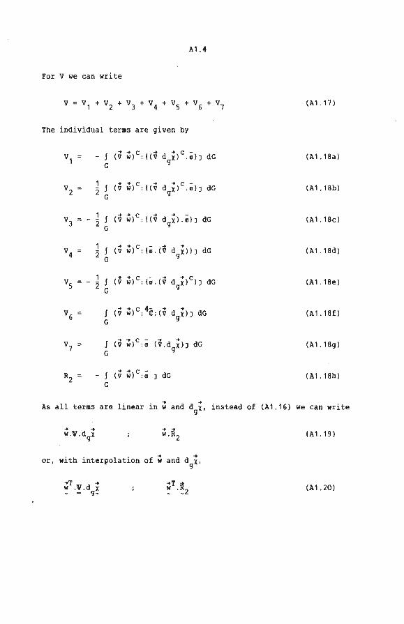
A1. 4
For V we can write
The individual terms are given by
1 ~ ~ c ~ ~ c -2 J (V w) : {(V dgx) . GJ}) dG G
1 ~ ~ c - ~ ~ 2 J (V w) : (a . (V dgxllJ dG G
.... c - ... ... f (V w) :111 (V.dgx)J dG G
- f <v ~lc : ; J dG G
(A 1. 17)
(A1.18a)
(A1.18b)
(A1.18c)
(A1 . 18d)
(A1.18e)
(A1.18f)
(A1.18g)
(A1.18h)
As all terms are linear in~ and dgx' insteadof (A1.16) we can write
~ ~
or, with interpolation of w and d9
x,
~T ~ w .V.d x ~ - g~
{A 1. 19)
(A1.20)
A2.1
Appendix 2: An iterative constitutive equation for time-independent
elasto-plastic material behaviour
The derivation of the constitutive equation starts from the
relationship between the Cauchy stress tensor ~ and the co-rotational
Cauchy stress tensor i, that is
Cl = IR.i .IRc (A2. 1)
where IR is the rotation tensor in the polar decomposition of the
deformation tensor F. It is easily shown that the linearised
expression for the iterative MRS change of ~ is given by
(A2 . 2)
From the definition (II.2.44) of the Green-Lagrange strain tensor
and the definition (II .2 .43) of the polar decomposition of the
deformation tensor F, it follows that
(A2.3)
Using the Cayley-Hamilton theorea it is shown in appendix 3 that
1 ([ + 2E)-Ï = c2E.E + c 1E + c0[ (A2.4)
where the scalar quantities c0 , c1 and c2 will depend on the
invariants of E. Now it is assumed that E is small coapared to the
unit tensor l
IIEII « 1 (A2.5)
In that case we can write
3 1 c 2 [ - 2 F .F (A2.6)

A2.2
and thus for R
IR 3 1 c 2 1F- 2 f.f .f (A2 . 7)
Some simple manipulation results in
d IR IRic m '
1 (d lH d ..,c) 2 m - m111 (A2.8)
In section V. 4 for i in state 1 the following expression has been
derived
i = K i + ! tr(GJ(T0
)) [ + K tr(G:) [ n 3
(A2.9)
Hence
d i d K . i + Kid G + K tr(dma:) [ GJ m m n m n (A2 . 10)
From the · definition (V.4.19) of the scalar quantity K we find
.a
=~~ K = _x
à i : i ê n n n
n
it follows after linearisation that
d K m
i a d a J. (~~i l. a a n v
d à ~)
.l. a
n
(A2. 11)
(A2 .12)
Using (V·. 4 . 6) the MRS change of the current yiel d stress av is gi ven
by
a V
:D (A2 . 13)
and from this, for the first term on the right- hand side of (A2.12),
we arrive at
d 0 m v
A2.3
. :dm~
(1 + ~)Ó~ (A2. 14)
For the second term on the right-hand side of (A2.12) we note that
from the definition (V.4.17) of in' it follows that
(A2. 15)
and therefore the MRS change of in becomes
d iJ 2G d ~d m n m (A2.16)
With the definition (A2.11) of on and (A2.15) it is seen that
3Gil .d 0 ___n
0 ;()
n (A2.17) n
From this we arrive at
3GIÎi d ó ___n :d ~d
m n .i m (A2.18) 0
n
Substituting (A2.14) and (A2.18) in (A2.12) results in
hiii i 3Gii 0
:d ~d dllll< :d ~ ...Y.. ___n
+ ~~-i2 m .i .i2 m ( 1 0 0
JG 0 n n n
(A2. 19)

and, using
d cÎI m
A2.4
(A2 .10) leaves US with
hi.i.i i QJ GJ 0
2G( 4[ n !l :d a: + _y
ll~:yi2 .i m (1 + 3G 0 n
0 n
+ K [ [:d «: m
.i. i 3 GJ GJ
~d _n_n - 2 .i2 l: dm 0 n
Replacing d ~d by m
1 dm[ - 3 tr(dmG:)[, we finally arrive at
d cÎI m
where the fourth-order tensor 4Mi is defined by
. . with the quantities G and P as
i hiöi 0 . a G _y p 1 - n .~ 0 3G( 1 n +
.i. i GJ GJ .....n....n) .i2 0
n
hi i 3G 10v
(A2.20)
(A2. 21)
(A2.22)
(A2.23)
The last term to be considered is the MRS change of the logarithmic
strain tensor a:, defined by
1 2ln([ + 21E) (A2.24)
In appendix 3 it is shown that
(A2.25)
Assuming I IIE 11 « 1 we find
(A2.26)
A2.5
(A2.27)
d b ri ~ Ri l' f an , ecause "' ~ IIEII « 1, also
(A2.2B)
Substituting (A2 . 28) in (A2.21) we find
(A2.29)
Premultiplying by Ri and postmultiplying by Ric gives
(A2.30)
where ~i is defined by
(A2. 31)
Substituting (A2.B) and (A2.30) in (A2.2) finally results in the
desired iterative constitutive equation
(A2.32)
A3 .1
Appendix 3: Functions of a tensor
Insome cases the value of the function f(A), where A is a second
order tensor, can be determined fairly easily by employinq the
Cayley-Hamilton theorem
(A3 . 1)
Here, J 1, J 2 and J 3 are the invariantsof A, defined by
J 1 = tr(A) J 3 det(A) (A3.2)
Repeated use of (A3.1) results in
(A3 . 3)
where the coefficients an' pn and yn are qiven by
ao 0 Po 0 Yo
a1 0 p1 y1 0
a2 p2 0 y2 0
aJ J1 PJ -J2 YJ JJ
-----------------------------a an-1J1 - an-2J2 + an-JJJ n pn - an-1J2 + an-2J3
Yn an-1J3 (A3 . 4)
If A is symmetrical, we can determine the coefficients a0 , a 1 and a2 in such a way that, for f(A), the expression
applies. On account of its sy .. etry, A can be written as
3 A= [
i=1
.. .. A.n.n. ~ ~ ~
(A3.5)
(A3.6)
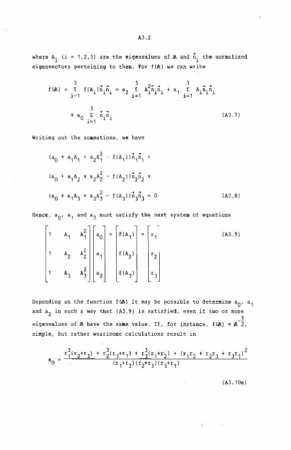
A3.2
where A. (i= 1,2,3) are the eigenvalues of~ and ~- the normalized 1 1
eigenveetors pertaining to them. For f(~) we can write
f(~)
3 r
i=1 f(A. )~ - ~ .
1 1 1
3 + a0 r
i=1
.. .. n.n .
1 1
Writing out the summations, we have
lao + a 1A1 2
+ a2A1 -.. ..
fiA 1 lln 1n1 +
2 .. .. (ao + a
1A
2 + a2A2 - f(A 2Jln2n2 +
ta0 + a 1A3 + 2 a2A3
.. .. f(A 3)ln3n3 0
(A3 . 7)
(A3.8)
Hence, a0 , a 1 and a2 must satisfy the next system of equations
A1 A2 1 ao fiA 1) r, (A3 . 9)
A2 A2 2 a, f(A 2 l r2
A3 A2 3 a2 f(A 3) r3
De pending on the function f (JA) it may be possible to determine ao,
and a2 in such a way that (A3.9) is satisfied, even if two or more
1 eigenvalues of~ have the same value. If, for instance, f (JA) = JA -21 simple, but rather wearisome calculations result in
(A3 .10a)
a,

A3.3
(A3 . 10b)
(A3. 10c)
It is easily shown that
(A3.11a)
2a 1 + 4a2 (A3 . 11b)
If ~ is not symmetrical or if a general valid solution for (A3.9)
cannot be determined, the following metbod for calculating f(~) can
be used, if f(~) is the sum of àn infinite, convergent series, that
is, if
f(~)
.. [
n=O
Using (A3.3) this results in
(A3.12)
(A3.13)
where, on account of (A3.4) the coefficient5 b0 , b1 and b2 are given
by
ho so + [ 5nln n=3
(A3. 14a)
b1 51 + [ 5npn n=3
(A3.14b)
b2 52 + [ 5 a n=3 n n (A3.14c)
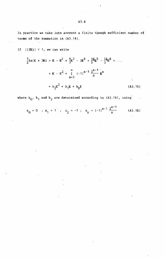
A3.4
In practice we take into account a finite though sufficient number of
termsof the summatien in (A3 . 14).
If II2EII < 1 ' we · can write
~ln([ + 2E) = IE - IE2 + 1E3 - 2E4 + ~5 - ~6 + ... 3 5 3
= E - IE2 + ( _1 )n-1
n-1 · r _2_ IEn
n=3 n
b IE 2 + 2 b1E + bo[ (A3.15)
where b0 , b1 and b2 are determined according to (A3 . 14), using
0 1 . -1 5 n
n-1 (-1)n-1 _2_
n (A3 . 16)
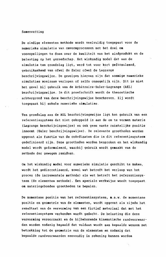
Samenvatting
De eindige elementen methode wordt veelvuldig toegepast voor de
numerieke simulatie van omvormprocessen met het doel om
voorspellingen te doen over de kwaliteit van het eindprodukt en de
belasting op het gereedschap. Het wiskundig model dat aan de
simulatie ten grondslag ligt, werd tot voor kort geformuleerd,
gebruikmakend van ofwel de Euler ofwel de Lagrange
beschrijvingswijze . De gevolgen hiervan zijn dat sommige numerieke
simulaties moeizaam verlopen of zelfs onmogelijk zijn . Dit is niet
het geval bij gebruik van de Arbitraire-Euler- Lagrange (AEL)
beschrijvingswijze . In dit proefschrift wordt de theoretische
achtergrond van deze beschrijvingswijze beschreven . Zij wordt
toegepast bij enkele numerieke simulaties.
Ten grondslag aan de AEL beschrijvingswijze ligt het gebruik van een
referentiesysteem dat niet gekoppeld is aan de om te vormen materie
(Lagrange beschrijvingswijze) en ook geen vaste ruimtelijke positie
inneemt (Euler beschrijvingswijze). De relevante grootheden worden
opgevat als functie van de coördinaten die in dit referentiesysteem
gedefinieerd zijn . Deze grootheden worden besproken en het wiskundig
model wordt geformuleerd, waarbij gebruik wordt gemaakt van de
methode der gewogen residuen .
Om het wiskundig model voor numerieke simulatie geschikt te maken,
wordt het gediscretiseerd, zowel wat betreft het verloop van het
proces (de incrementele methode) als wat betreft het referentiesys
teem (de elementen methode). Een speciale werkwijze wordt toegepast
om materiegebonden grootheden te bepalen .
De momentane positie van het referentiesysteem, m.a.w. de momentane
positie en geometrie van de elementen, wordt opgevat als zijnde het
resultaat van de vervorming van een fictief materiaal dat met het
referentiesysteem verbonden wordt gedacht . De belasting die deze
vervorming veroorzaakt en de bijbehorende kinematische randvoorwaar
den worden zodanig bepaald dat voldaan wordt aan bepaalde wensen met
betrekking tot de geometrie van de elementen en zodanig dat
bepaalde randvoorwaarden eenvoudig in rekening kunnen worden

gebracht. De vervorming van reêel en fictief materiaal vindt
gelijktijdig plaats.
Het gediscretiseerd wiskundig model bestaat uit een stelsel niet
lineaire algebraische vergelijkingen. De onbekende grootheden worden
bepaald volgens een iteratieve methode. Daarbij wordt een aantal
benaderingen van de uiteindelijke oplossing bepaald door herhaald
oplossen van de gelineariseerde versie van bovengenoemd stelsel .
De AEL beschrijvingswijze is met succes toegepast voor de simulatie
van enkele axi-symmetrische omvormprocessen.
Nawoord
Het in dit proefschrift beschreven onderzoek is van februari 1979 tot
augustus 1983 uitgevoerd binnen de vakgroep Fundamentele Werktuigbouw
kunde (voorheen Technische Mechanica) van de Technische Hogeschool
Eindhoven.
De initiator van het onderzoek was Joop Nagtegaal, In de beginfase had
ik in hem een enthousiast en deskundig begeleider. Toen Joop de TH
verliet, werd zijn begeleidende taak overgenomen door Frans Veldpaus
en Marcel Brekelmans. De vanzelfsprekendheid waarmee en de manier
waarop dit gebeurde verdient bewondering. Het resultaat van de vele
gesprekken die we samen gevoerd hebben is in het proefschrift aanwijs
baar aanwezig in de vorm van ideeën en formuleringen. Bij veel van deze
besprekingen was de regulerende invloed van Jan Janssen van groot
belang.
Van groot nut is het afstudeerwerk van Martien Hulsen geweest. Hij
paste de AEL beschrijvingswijze toe voor de simulatie van hyper
elastische vervormingsprocessen.
Het proefschrift is getypt door Lia Neervoort en Els Scheepens. Vooral
Els heeft bereidwillig vele uren doorgebracht achter de terminal van
het tekstverwerkingsysteem om op zeer accurate wijze de vele
wijzigingen in de tekst aan te brengen. Marcel Brekelmans heeft het
uiteindelijke manuscript grondig bekeken, hetgeen nog een aantal
verbeteringen tot gevolg had.
Bovengenoemde personen wil ik hartelijk bedanken voor de bijdrage aan
het onderzoek en de totstandkoming van het proefschrift en vooral ook
voor de plezierige wijze waarop de samenwerking plaatsvond.
Behalve de hierboven met name genoemde personen, wil ik alle leden van
de vakgroep Fundamentele Werktuigbouwkunde bedanken voor de prettige
contacten. Mede als gevolg hiervan heb ik binnen deze vakgroep een
aantal jaren fijn gewerkt
Eindhoven, augustus 1983
Piet Schreurs
STELLINGEN
behorende bij het proefschrift
NUMERICAL SIMULATION OF FORMING PROCESSES
I. De in dit proefschrift beschreven Arbitraire-Euler-Lagrange
formulering is een geschikt uitgangspunt om bij gebruik van de
eindige elementen methode (automatisch) de elementverdeling te
optimaliseren en om zowel materiegebonden als niet-materiegebonden
randvoorwaarden eenvoudig in rekening te brengen .
Hoofdstuk VII van dit proefschrift.
2. Bij simulatie van omvormprocessen met behulp van de eindige elementen
methode is optimaliseren van de elementverdeling in veel gevallen
alleen goed mogelijk als het aantal elementen tijdens de simulatie
kan worden veranderd.
3. De in dit proefschrift beschreven methode voor de berekening van
materiegebonden grootheden in een niet-materiegebonden element
verdeling leidt, in vergelijking met de gebruikelijke werkwijze
bij de Lagrange formulering, in het algemeen tot een lagere
convergentiesnelheid.
Hoofdstuk VII van dit proefschrift.
4. Voor de simulatie van vloeistofstromingsprocessen met behulp van
de eindige elementen methode is de beschrijving van het proces in
termen van stroomsnelheid en (eventueel) hydrostatische druk te
prefereren boven de beschrijving in termen van stroomfunctie en
wervelsterkte.
5. Bij de beschrijving van de stroming van incompressibele vloei
stoffen in termen van stroomsnelheid en hydrostatische druk blijkt
de Lagrange multiplicator, waarmee de incompressibiliteitseis
meestal in rekening wordt gebracht, geÏdentificeerd te kunnen worden
met de hydrostatische druk. Dit impliceert dat, als bij toepassing
van de elementen methode de druk in een knooppunt wordt voorgeschreven,
lokaal niet meer kan worden voldaan aan de continuiteitsvergelijking.
Gresho P.M., Lee R.L., Sani R.L.: On the time-dependent salution
of the incompressible Newton-Stakes equations in two and three
dimensions. Recent advances in numerical methods in fluids
(ed. C. Taylor and K. Morgan), Pineridge Press Ltd., Swansea,
U.K., pp. 27-79, 1980.
6. Roll en Neitzert negeren de mogelijkheid om de eindige elementen
methode af te leiden met behulp van de methode der gewogen residuën.
Roll K., Neitzert T.: On the application of different numerical
methods to calculate cold forrning processes. Numerical methods
in industrial forming processes, Swansea, U.K., juni 1982.
7. Het begrip initiële rek is fysisch niet zinvol. Gebruik van dit
begrip is verwarrend en moet vermeden worden.
8. De uit militaire kringen voortkomende, ongegronde verdachtmakingen
aan het adres van de vredesbeweging vormen de beste propaganda
die deze beweging zich wensen kan.
9. Het toenemend aanbod van voedingsmiddelen in voordeelverpakking zal
de noodzakelijke gevarieerdheid in de voeding verminderen.
10. Door automatisering gaat werk naar de knoppen.
Eindhoven, 12 september 1983 Piet Schreurs