NUMERICAL SIMULATION OF FLOATING OFFSHORE WIND …
147
NUMERICAL SIMULATION OF FLOATING OFFSHORE WIND TURBINE DYNAMIC RESPONSES WITH EXPERIMENTAL COMPARISON A Dissertation by HYUNSEONG MIN Submitted to the Office of Graduate and Professional Studies of Texas A&M University in partial fulfillment of the requirements for the degree of DOCTOR OF PHILOSOPHY Chair of Committee, Jun Zhang Co-Chair of Committee, Hamn-Ching Chen Committee Members, Moo-Hyun Kim David Arthur Brooks Head of Department, Sharath Girimaji May 2018 Major Subject: Ocean Engineering Copyright 2018 Hyunseong Min
Transcript of NUMERICAL SIMULATION OF FLOATING OFFSHORE WIND …

NUMERICAL SIMULATION OF FLOATING OFFSHORE WIND TURBINE
DYNAMIC RESPONSES WITH EXPERIMENTAL COMPARISON
A Dissertation
by
HYUNSEONG MIN
Submitted to the Office of Graduate and Professional Studies of
Texas A&M University
in partial fulfillment of the requirements for the degree of
DOCTOR OF PHILOSOPHY
Chair of Committee, Jun Zhang
Co-Chair of Committee, Hamn-Ching Chen
Committee Members, Moo-Hyun Kim
David Arthur Brooks
Head of Department, Sharath Girimaji
May 2018
Major Subject: Ocean Engineering
Copyright 2018 Hyunseong Min

ii
ABSTRACT
Hywind, the world’s first operational Floating Offshore Wind Turbine (FOWT),
is constrained by a delta mooring system to improve the yaw station-keeping capacity. In
this study, a mooring line-simulation code in COUPLE-FAST was extended to simulate
the dynamics of a delta mooring system using a Finite Element Method. The old mooring-
simulation code in COUPLE-FAST was replaced with the extended code, and the new
program is named as COUPLE-D-FAST. In this program, FAST calculates the
aerodynamic, control and electrical system, and structural dynamic forces. COUPLE-D
computes mooring and hydrodynamic forces, and then it calculates the global motions of
FOWT using the wind forces computed using FAST.
COUPLE-D-FAST was then employed for the simulation of Hywind constrained
by a taut delta mooring system. The simulated global motions and mooring lines’ tensions
of Hywind were compared with the related measurements in a wave basin and the
corresponding simulations obtained using a commercial code, FAST-OrcaFlex.
Several cases were simulated and compared with the measurements, which include
free-decay tests, wind loads-only tests, wave loads-only tests, and wind combined with
wave loads tests. Without empirical tunings on the yaw stiffness and damping of the
Hywind’s mooring system, the simulated yaw free-decay responses showed excellent
agreement with those of the model test. In general, the simulated motions and mooring
lines’ tensions of Hywind showed satisfactory agreement with the experimental results in
the cases of various wind and wave conditions. For the cases of wind combined with
iii
irregular wave loads, however, the simulated pitch of the FOWT near its resonant
frequency was significantly smaller than the related measurements. This may result from
the scaling issue between the prototype and its model that the aerodynamic damping
follows the Reynolds number while the scale in the model test was based on the Froude
number.
In this dissertation, it was found that COUPLE-D-FAST can reliably and
accurately simulate the delta mooring system of Hywind. The accurate predictions of the
delta mooring dynamics may make important contribution to the future design of FOWT.

iv
ACKNOWLEDGEMENTS
I would like to express my gratitude to Dr. Jun Zhang, my advisor and my
committee chair, for his profound comments and suggestions throughout this research. I
also would like to thank my committee co-chair, Dr. Hamn-Ching Chen, and my
committee members, Dr. Moo-Hyun Kim and Dr. David Brooks, for their guidance and
support throughout the course of this research.
I want to thank Dr. Cheng Peng for providing the source code of COUPLE-FAST
and sharing his knowledge of the numerical challenges of coupling problems. Thanks also
go to my friends and colleagues and the department faculty and staff for making my time
at Texas A&M University a great experience.
Finally, special thanks to my mother, father and brother for their encouragement
and unfailing support. I want to express my deepest love and thanks to my wife, Soonwoo
Kim, for her patience, love, and taking care of our son. I am thankful to my son Henry for
giving me happiness.

v
CONTRIBUTORS AND FUNDING SOURCES
Contributors
This work was supervised by a dissertation committee consisting of Professors Jun
Zhang and Hamn-Ching Chen of the Department of Civil Engineering, Professor Moo-
Hyun Kim of the Department of Ocean Engineering, and Professor David Arthur Brooks
of the Department of Oceanography.
The model test data for Chapters 4 to 6 were provided by State Key Laboratory of
Ocean Engineering in Shanghai Jiao Tong University.
All other work conducted for the dissertation was completed by the student
independently.
Funding Sources
Graduate study was supported by scholarships from the Department of Ocean
and a dissertation fellowship from Office of Graduate and Professional Studies at Texas
Engineering at Texas A&M University and Barrett and Margaret Hindes Foundation,
A&M University.

vi
NOMENCLATURE
CG Center of Gravity
DOE U.S. Department of Energy
DOF Degrees of Freedom
FEM Finite Element Method
FFT Fast Fourier Transform
FOWT Floating Offshore Wind Turbines
HWM Hybrid Wave Model
IFFT Inverse Fast Fourier Transform
JONSWAP Joint North Sea Wave Project
KC Keulegan-Capenter
LC Load Case
LF Low Frequency
MARIN Maritime Research Institute Netherland
NREL National Renewable Energy Laboratory
OC3 Offshore Code Comparison Collaboration
TLP Tension Leg Platform
WF Wave Frequency

vii
TABLE OF CONTENTS
Page
ABSTRACT .......................................................................................................................ii
ACKNOWLEDGEMENTS .............................................................................................. iv
CONTRIBUTORS AND FUNDING SOURCES .............................................................. v
NOMENCLATURE .......................................................................................................... vi
TABLE OF CONTENTS .................................................................................................vii
LIST OF FIGURES ........................................................................................................... ix
LIST OF TABLES ...........................................................................................................xii
1. INTRODUCTION ........................................................................................................ 1
1.1. Background and Literature Review ............................................................... 1 1.2. Overview of the Research Work .................................................................... 9
2. DYNAMICS OF A DELTA MOORING SYSTEM .................................................. 11
2.1. Dynamic Equations for an Extensible Mooring Line .................................. 11
2.2. Numerical Implementation: Finite Element Method ................................... 12 2.3. Boundary Conditions ................................................................................... 17
2.3.1. Boundary Conditions at the Smooth Connections ..................... 17
2.3.2. Boundary Conditions at the Jointed Connections ...................... 18 2.4. Formulation .................................................................................................. 19
3. PRINCIPLES OF COUPLE-D-FAST ....................................................................... 22
3.1. Modeling of FOWT in COUPLE-D ............................................................ 22 3.2. Modeling of FOWT in FAST ...................................................................... 25
3.2.1. Wake and Airfoil Modeling ....................................................... 26 3.2.2. Blade and Tower Flexibility ...................................................... 26 3.2.3. Control System........................................................................... 27
3.3. Coupling Overview of COUPLE-FAST ...................................................... 27 3.3.1. Coordinate Systems ................................................................... 29
3.3.2. Mathematical Formulation of Coupling Problem ...................... 33 3.3.3. Coupling Procedures of COUPLE-D-FAST .............................. 35
4. NUMERICAL MODEL SET-UP AND CALIBRATION ......................................... 38

viii
4.1. Model Experiments ...................................................................................... 38 4.1.1. Experimental Facilities .............................................................. 38
4.1.2. Set-up of Model and Instruments ............................................... 39 4.2. Numerical Simulation Set-up and Calibration ............................................. 42
4.2.1. Simulation Settings .................................................................... 42 4.2.2. Hywind Platform Model ............................................................ 43 4.2.3. Hydrodynamic Coefficients for the Morison Equation ............. 44
4.2.4. Tower Stiffness Tests ................................................................. 45 4.3. Fixed Wind Turbine Test ............................................................................. 46
5. INVESTIGATION OF HYWIND RESPONSES ...................................................... 48
5.1. Mooring Stiffness Test ................................................................................. 48 5.2. Free-decay Tests .......................................................................................... 52
5.2.1. Free-decay Tests without Tuned Parameters ............................. 52 5.2.2. Free-decay Tests with Adjusted Parameters .............................. 56
5.3. Corrections of Wind Speeds ........................................................................ 59 5.4. Motions of Hywind under Steady Wind Loads ........................................... 61
5.5. Discussion .................................................................................................... 64
6. INVESTIGATION OF HYWIND RESPONSES WITH CORRECTED CENTER
OF GRAVITY ............................................................................................................ 65
6.1. Environmental Conditions ........................................................................... 65 6.1.1. Turbulent Wind Conditions ....................................................... 65
6.1.2. Met-ocean Conditions ................................................................ 67 6.2. Correction of the Center of Gravity ............................................................. 68
6.2.1. Simulation using Measured Wind Forces .................................. 68 6.2.2. Correction of the Center of Gravity ........................................... 71
6.3. Free-decay Tests .......................................................................................... 74 6.4. CASE I: Turbulent Winds Impact-Only Cases ............................................ 80 6.5. CASE II: Waves Impact-Only Cases ........................................................... 83
6.5.1. Wave Generation ....................................................................... 83 6.5.2. Simulation Results ..................................................................... 85
6.6. CASE III: Impact of Turbulent Winds and Regular Waves ........................ 94
6.7. CASE IV: Impact of Turbulent Winds and Irregular Waves ..................... 102 6.8. Discussion .................................................................................................. 109
7. CONCLUSIONS ...................................................................................................... 111
REFERENCES ............................................................................................................... 116
APPENDIX A ................................................................................................................ 121
ix
LIST OF FIGURES
Page
Figure 1 Cumulative Installed Wind Power Capacity Required to Produce 20% of
Projected Electricity by 2030; Reprinted from U.S.DOE (2008) ....................... 2
Figure 2 Delta Mooring System ......................................................................................... 6
Figure 3 Discretization of a Cable .................................................................................... 11
Figure 4 Boundary Conditions of Delta Mooring System ............................................... 17
Figure 5 Assembled Matrix for a Cable with N Elements ............................................... 21
Figure 6 Assembled Matrix for a Delta Mooring System ................................................ 21
Figure 7 Wave Frequency Band Division; Reprinted from Zhang et al. (1996) .............. 25
Figure 8 Flowchart of Coupling Procedure of COUPLE-D-FAST .................................. 29
Figure 9 Coordinate Systems of Hywind in COUPLE-D-FAST ..................................... 30
Figure 10 xy-Plane View of Space-fixed Coordinate System .......................................... 31
Figure 11 Body-fixed Coordinate Systems ...................................................................... 32
Figure 12 Flow Chart of Simulation Process in COUPLE-D-FAST ............................... 37
Figure 13 Model Setting (a) and Floating Platform (b); Reprinted from Duan et al.
(2015) ................................................................................................................ 40
Figure 14 Mooring Layout (a) and Assembled Devices (b); (b) is reprinted from Duan
et al. (2015) ....................................................................................................... 41
Figure 15 Geometry of Hywind Spar ............................................................................... 43
Figure 16 Taper Modeling in the Simulation ................................................................... 44
Figure 17 Mooring Layouts in the Simulations ............................................................... 49
Figure 18 Static Offset Test Comparisons; (a) and (d) are reprinted with permission
from Min and Zhang (2017) ............................................................................. 50
Figure 19 Configuration of Mooring Lines (Yaw=10°); Reprinted with permission
from Min and Zhang (2017) ............................................................................. 51

x
Figure 20 Free-decay Tests in Translational Directions (Un-tuned); (a) and (c) are
reprinted with permission from Min and Zhang (2017) ................................... 54
Figure 21 Free-decay Tests in Rotational Directions (Un-tuned); (c) is reprinted with
permission from Min and Zhang (2017) ........................................................... 55
Figure 22 Free-decay Tests in Rotational Directions (Tuned); (c) is reprinted with
permission from Min and Zhang (2017) ........................................................... 58
Figure 23 Initial Settings of Rotor in SJTU’s Study; Reprinted with permission from
Min and Zhang (2017) ...................................................................................... 59
Figure 24 Average Platform Motions and Mooring Tensions ......................................... 63
Figure 25 Comparison of Surge and Pitch Amplitude Spectrum (Operational 1) ........... 67
Figure 26 Comparison of Surge and Pitch Amplitude Spectrum (Operational 2) ........... 67
Figure 27 Comparison of Surge and Pitch Amplitude Spectrum (Extreme) .................... 67
Figure 28 Average Platform Motions using Measured Wind Forces ............................... 70
Figure 29 Pitch Decay Results with the Given (blue) and Corrected (red) CG ............... 72
Figure 30 Average Platform Motions using Measured Wind Forces with the Corrected
CG ..................................................................................................................... 73
Figure 31 Free-decay Tests in Rotational Directions (Tuned) ......................................... 75
Figure 32 Mooring Layout for Indexing .......................................................................... 77
Figure 33 Downstream-side Mooring Tension during Yaw Free-decay .......................... 78
Figure 34 Upstream-side Mooring Tension during Yaw Free-decay............................... 79
Figure 35 Average Platform Motions and Mooring Tensions (LC01-LC03) .................. 81
Figure 36 Wave Elevations (LC05) ................................................................................. 84
Figure 37 Spectrum of Wave Elevations (LC05) ............................................................. 84
Figure 38 Comparison of Platform Motions (LC04) ....................................................... 87
Figure 39 Comparison of Simulated Motions (LC04) ..................................................... 88
Figure 40 Comparison of Mooring Tensions at Delta Joint (LC04) ................................ 89

xi
Figure 41 Comparison of Platform Motions (LC05) ....................................................... 92
Figure 42 Comparison of Mooring Tensions at Delta Joint (LC05) ................................ 93
Figure 43 Average Platform Motions and Mooring Tensions (LC06-LC08) .................. 96
Figure 44 Amplitudes of Platform Motion and Mooring Tension at WF (LC06-LC08) . 97
Figure 45 Comparison of Platform Motions (LC08) ..................................................... 100
Figure 46 Comparison of Mooring Tensions at Delta Joint (LC08) .............................. 101
Figure 47 Comparison of Tower-top Yaw Moments (LC08) ........................................ 102
Figure 48 Comparison of Platform Motions (LC11) ..................................................... 106
Figure 49 Comparison of Mooring Tensions at Delta Joint (LC11) .............................. 107
Figure 50 Comparison of Tower-top Yaw Moments (LC11) ........................................ 108

xii
LIST OF TABLES
Page
Table 1 Mass Properties of Hywind Model (Duan et al., 2015) ...................................... 41
Table 2 Platform Properties of Hywind Model ................................................................ 41
Table 3 Mooring System Properties; Reprinted from Duan et al. (2015) ........................ 42
Table 4 Parameters for Estimation of Drag Coefficient ................................................... 45
Table 5 Fixed Wind Turbine Test Results; Reprinted from Duan et al. (2015) ............... 47
Table 6 Adjusted Parameters of the FOWT System ........................................................ 56
Table 7 Natural Period of Hywind FOWT; Reprinted with permission from Min and
Zhang (2017) .................................................................................................... 57
Table 8 Redefined Wind Speed; Reprinted with permission from Min and Zhang (2017)
.......................................................................................................................... 60
Table 9 Average Behaviors of Hywind by Steady Wind Impact; Reprinted with
permission from Min and Zhang (2017) ........................................................... 62
Table 10 Average Behaviors of Hywind by Steady Wind Impact; Reprinted from Min
et al. (2016) ....................................................................................................... 63
Table 11 Wind Speeds ...................................................................................................... 66
Table 12 Environmental Conditions ................................................................................ 68
Table 13 Environmental Conditions for Simulations using Measured Wind Forces ....... 70
Table 14 Pitch Moment of Inertia and Stiffness Comparison .......................................... 72
Table 15 Additional Tuning of the FOWT System .......................................................... 74
Table 16 Natural Period of the Hywind System (Unit: sec) ............................................ 76
Table 17 Averages of Platform Motions and Mooring Tensions (LC01-LC03) .............. 82
Table 18 Statistics for Platform Motions and Mooring Tensions (LC04) ....................... 86
Table 19 Statistics for Platform Motions and Mooring Tensions (LC05) ....................... 91

xiii
Table 20 Averages and Amplitudes of Platform Motions and Mooring Tensions (LC06-
LC08) ................................................................................................................ 95
Table 21 Statistics for Platform Motions and Mooring Tensions (LC09-LC11) ........... 105

1
1. INTRODUCTION
1.1. Background and Literature Review
For the last two decades, the world’s level of renewable energy use has grown to
meet our current and future energy needs. Among the various types of renewable energy,
wind is one of the most widely available and cost-effective sources. In the past, most wind
turbines were primarily constructed on land or in nearshore water. However, such turbines
have shortcomings such as visual and noise impacts on residents, and intermittent
electricity generation due to fluctuating wind speeds. Offshore wind turbines, especially
those located in relatively deep water, can alleviate these problems. Especially since
offshore wind tends to get stronger and steadier as the distance from land increases, such
locations are likely to increase the production of electricity.
In 2008, the US Department of Energy (DOE) published a report stating that wind
energy could provide as much as 20% of the US’s electricity by 2030. This would have a
positive effect on the environment by reducing air pollutants and carbon dioxide emissions.
A shift to wind energy would also help to conserve water and reduce the demand for fossil
fuels. As shown in Figure 1, offshore wind technology could gradually increase to
generate as much as 18% (54GW) of the total wind power capacity by 2030 (U.S.DOE,
2008).
In the United States, wind power capacity increased by 8.2GW in 2016. Wind
capacity increased to the total constructed wind capacity of 82.1GW. In the same year,
global wind additions were estimated at 54.6GW, for a cumulative total of 486.7GW. The

2
US’s wind energy market took second place behind China, based on the cumulative
capacity. The first offshore wind farm in the United States was commissioned in Rhode
Island in December of 2016. The projected capacity is 30 MW, and it is expected to supply
electricity to 17,000 Rhode Island households (U.S.DOE, 2017a, b).
Figure 1 Cumulative Installed Wind Power Capacity Required to Produce 20% of
Projected Electricity by 2030; Reprinted from U.S.DOE (2008)
Designing and constructing offshore wind farms is quite difficult compared to on-
land production. Construction costs are high because offshore structures must endure
harsh conditions such as hurricanes and typhoon. In addition, offshore wind turbines
demand relatively high maintenance costs compared to those on land. Despite these
disadvantages, offshore wind sources generate more energy because the offshore winds
quality is better than those on land. According to the National Renewable Energy
Laboratory (NREL), US offshore wind sources could generate as much as four times the
nation’s electric capacity (Musial and Ram, 2010).

3
Currently, several countries have plans to construct or been constructing floating
wind farms. Floating Offshore Wind Turbines (FOWT) have already been built in many
locations. The world’s first operational FOWT was called Hywind; it was constructed by
Statoil of Norway. The floating platform is a spar-buoy type with 100 m draft and installed
in 200 m water depth. The diameter of the platform is 8.3 m at the main section and 6 m
at the water’s surface. The platform is connected to the seabed through a three-point
mooring system. The wind turbine has a capacity of 2.3 MW and produced 32.5 GWh
since 2010. Recently, Statoil constructed the world’s first wind farm, named Hywind
Scotland Pilot Park located in Scotland. The wind turbines were installed at a water depth
of 95 to 129 m. They have a capacity of 30 MW in total, which could provide around
22,000 homes with electricity beginning in late 2017.
The second FOWT built was called WindFloat. The FOWT is a semi-submersible
designed by Principle Power, and it was constructed in the offshore of Portugal in 2011.
This structure’s design was intended to improve motion performance by including heaving
plates at each column. Thus, the structure is able to set aside stability by establishing a
sufficiently low pitch motion. Chain and polyester mooring lines are deployed in the
pursuit of cost effectiveness and simplicity. The wind turbine has a 2 MW capability; it
generated 3 GWh of power the year after its construction (www.principlepowerinc.com).
Another FOWT has been in operation since 2013 on offshore Nagasaki, Japan
(Utsunomiya et al., 2015). Its type of platform is a hybrid-spar buoy, and it supports 2
MW of downwind-type turbines. The platform consists of a steel and precast pre-stressed
concrete. The diameter of the platform is 7.8 m at the main section and 4.8 m at the water’s

4
surface. The hub height is 56 m above the water’s surface, and the draft is 76 m. The
platform is attached to the seabed by three anchored chains. Fukushima Shinpuu FOWT
was deployed in Fukushima, Japan in 2015. The platform is a V-shaped semi-submersible
with eight mooring lines; the wind turbine’s capacity is 7 MW, making it the world’s
largest floating wind turbine (www.fukushima-forward.jp).
Since structures of FOWTs in deep water are floaters, they must be constrained by
a mooring or tendon system. Because the mooring system plays an important role in the
floating structure’s movement, an accurate prediction of the mooring system’s behavior is
crucial. Several simulation tools have been developed to predict FOWT behavior, such as
HAWC2 and FAST. HAWC2 was developed by DTU Wind Energy of Denmark to
simulate FOWT responses. FAST was created by the National Renewable Energy
Laboratory (NREL), and it is one of the most well-known simulation tools. Through
Offshore Code Comparison Collaboration (OC3), the performance of FAST was
successfully verified against other numerical codes such as HAWC2 and Simo (Jonkman
and Musial, 2010).
Along with the development of FOWT simulation tools, several model tests were
conducted to understand FOWT motion characteristics, as well as to validate the related
numerical simulation tools. Hydro Oil & Energy tested a spar-type platform with a 5 MW
wind turbine at the Ocean Basin Laboratory of Marintek in Norway (Nielsen et al., 2006).
At the basin of the Maritime Research Institute Netherland (MARIN), model tests of a
1:50 scale were implemented for three different types of platforms: spar-buoy, semi-
submersible, and TLP-type coupled with the NREL 5MW baseline wind turbine (Goupee

5
et al., 2014). They provided the FOWT configurations, setup details, and measurement
sensors and devices. The different concepts of FOWTs were then compared under various
sea states and wind conditions (Koo et al., 2012). Recently, Hywind experiments were
conducted at the Deepwater Offshore Basin in Shanghai Jiao Tong University (SJTU) of
a 1:50 scale (Duan et al., 2015).
Despite the many numerical codes developed and model tests conducted, there
have been few published studies comparing the results of model tests and numerical
simulations. Regarding the 5MW wind turbine supported by the Hywind platform, Nielsen
et al. (2006) presented a comparison of predicted and measured surge motions at the
nacelle under various wind and wave conditions. Two different numerical codes
(HywindSim and Simo-Riflex) were used for the simulation, and they rendered similar
predictions. While the comparisons showed that the predicted surge motions in the wave
frequency range were close to the measurements, predictions in the range of resonant pitch
and surge frequencies were found to be significantly different (by 100% to 200%) from
the related measurements. More recently, Browning et al. (2012) conducted numerical
simulations using FAST and compared them to measurements of a 1:50 scaled model
(Hywind) made in the MARIN’s wave basin (Martin et al., 2012). After comparing the x-
axis direction acceleration at the top of the wind tower and heave of the spar, they showed
that the wave frequency predictions and measurements were close, but there were large
discrepancies in the resonant pitch and surge frequencies, consistent with observations
made in a previous study by Nielsen et al. (2006). It should be noted that no comparisons
of predicted and measured mean motions were presented in these two studies.
6
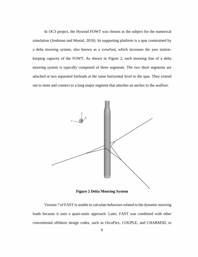
In OC3 project, the Hywind FOWT was chosen as the subject for the numerical
simulation (Jonkman and Musial, 2010). Its supporting platform is a spar constrained by
a delta mooring system, also known as a crowfoot, which increases the yaw station-
keeping capacity of the FOWT. As shown in Figure 2, each mooring line of a delta
mooring system is typically composed of three segments. The two short segments are
attached at two separated fairleads at the same horizontal level to the spar. They extend
out to meet and connect to a long major segment that attaches an anchor to the seafloor.
Figure 2 Delta Mooring System
Version 7 of FAST is unable to calculate behaviors related to the dynamic mooring
loads because it uses a quasi-static approach. Later, FAST was combined with other
conventional offshore design codes, such as OrcaFlex, COUPLE, and CHARM3D, to
X
Y
Z

7
utilize their ability to calculate dynamic mooring loads. Although FAST was coupled with
various offshore design codes, it still relied on empirical tunings on the yaw stiffness and
damping to simulate the delta mooring system. Several previous studies (Bae et al., 2011;
Browning et al., 2012; Min et al., 2016) used empirically calibrated increases in the yaw
stiffness and damping for the delta mooring system. Then the three segments of mooring
line were simplified to an equivalent conventional one-segment mooring line in the
simulations.
Efforts have been made to validate empirically calibrated increases in the yaw
stiffness and damping of a delta mooring system. Kallesøe and Hansen (2011) developed
a dynamic mooring line model, which was coupled with HAWC2. In their study, the delta
mooring system was analyzed using a multi-body formulation in HAWC2. The results
obtained using their program were compared to those obtained using a quasi-static
approach. They concluded that the bending equivalent loads at the bottom of the wind
tower computed by the direct modeling approach were less than those calculated by the
quasi-static approach. Quallen et al. (2013) introduced a quasi-static mooring model for
the delta mooring. Their codes were coupled with a CFD-based hydrodynamic simulation
code. They verified their code against the related results of OC3 (Jonkman and Musial,
2010) in free-decay and regular wave-only tests. Hall and Goupee (2015) developed a
lumped-mass mooring line model and verified it by comparing it to experimental results
from the DeepCWind, a semi-submersible FOWT. Their code could be used to simulate a
delta mooring system, and was utilized later by Andersen et al. (2016).

8
Various mooring analysis tools have been released in version 8 of FAST, including
Map++, MoorDyn, and FEAMooring. Map++ uses a quasi-static approach to model a
mooring system. MoorDyn employs a lumped-mass method, and FEAMooring applies a
Finite Element Method (FEM). The last two approaches (the lumped-mass method and
FEM) have also been used in commercial offshore design codes. Despite the many
numerical codes have been released for the mooring system analysis, very few are
specialized for the dynamic simulations of a delta mooring system. Wendt et al. (2016)
verified the applicability of the MoorDyn, FEAMooring, and Map++ mooring modules in
version 8 of FAST in the simulation comparing with DeepCWind test results. However,
they did not examine the delta mooring system. Andersen et al. (2016) focused on
validating the ability of version 8 of FAST to model the Hywind’s delta mooring system.
They used Map++ and MoorDyn to compare simulations obtained using FAST-OrcaFlex.
In their study, FEAMooring was not employed because it was unable to model a delta
mooring system directly. The simulation data for free-decay and wave-only tests were
compared with the OrcaFlex simulation and related measurements obtained from the
MARIN’s basin test. The results calculated by the dynamic mooring solver, MoorDyn,
showed a satisfactory level of agreement with those of OrcaFlex. They also found that the
direct modeling of a mooring system can provide far more accurate results regarding
mooring line tensions than the simplified mooring line approach with an empirically-
calibrated increase in yaw stiffness and damping.

9
1.2. Overview of the Research Work
In this research, COUPLE-D-FAST was developed allowing for the simulation of
a delta mooring system. It was then applied to the simulations of the Hywind FOWT. The
mooring module in COUPLE-D-FAST was developed using FEM, as in the case with
FEAMooring (Version 8 of FAST), but our software can simulate a delta mooring system.
The developed module was combined with existing code entitled COUPLE-FAST and
named COUPLE-D-FAST.
The main advantages of using COUPLE include the accurate prediction of
hydrodynamic and mooring loads. First, the Hybrid Wave Model (HWM) (Zhang et al.,
1996) was chosen to compute the wave kinematics, which led to accurate predictions of
nonlinear wave interactions. The ratio of the diameter of the Hywind platform to the wave
length at the spectral peak was small enough to allow for the slender-body approximation.
Thus, the wave loads (both potential and drag forces) were calculated by the Morison
equation, and the wave kinematics were predicted using the HWM. Since HWM was able
to predict the wave kinematics at a second order wave steepness up to the free surface,
there was no need to use an empirical stretch or approximation such as linear extrapolation
or wheeler stretching. Regarding the mooring dynamics in COUPLE-D, the delta mooring
system could then be explicitly modeled for a dynamic simulation. Hence, the yaw
stiffness and damping of a delta mooring system could be accurately calculated without
relying on empirical tunings.
This dissertation provides a description of how to model a delta mooring system;
using the case of Hywind FOWT with a taut delta mooring system. COUPLE-D-FAST

10
was employed to simulate the FOWT’s motion and tension in its mooring system. The
dynamic behaviors of the delta mooring system obtained using COUPLE-D-FAST were
then compared with the results of other existing codes such as COUPLE-FAST and FAST-
OrcaFlex, as well as the measurements of SJTU (Duan et al., 2015).

11
2. DYNAMICS OF A DELTA MOORING SYSTEM
For simulations of a delta mooring system, the CABLE3D module (Ma and
Webster, 1994), the mooring module in COUPLE, is modified. The mooring module is
based on FEM. It follows Garrett (1982)’s principle for an inextensible cable and Lindahl
and Sjoberg (1983)’s study for an extensible cable. The detailed derivation of the
governing equations for an extensible mooring line can be found in Chen (2002). In this
section, the governing equations and the numerical formulation especially for the delta
mooring system are described.
2.1. Dynamic Equations for an Extensible Mooring Line
Figure 3 Discretization of a Cable
In using FEM to compute mooring dynamics, an extensible mooring line can be
considered as the long slender cable, and the bending moments and shear forces are

12
neglected. As shown in Figure 3, the FEM discretizes the long slender cable into many
elements that each element has two nodes at both ends. Mooring line tension T is the only
internal force.
The configuration of a cable can be represented by a vector, r(s,t), where s and t
represent the arc length along the cable, and time, respectively. Based on the conservation
of linear momentum the governing equation can be expressed as follows together with a
stretching constraint condition:
qrrM )~
( (2.1)
1)
~
1( 2 EA
rr (2.2)
where, M is the mass matrix, is the Lagrange multiplier which can be expressed using
the normal strain ε and the tension in a cable, / (1 )T . q is the external forces
distributed on the cable; it includes hydrostatic, hydrodynamic and gravity forces. EA is
the axial stiffness of the cable. A superposed dot denotes the derivatives with respect to
time, and a prime the derivatives with respect to space.
2.2. Numerical Implementation: Finite Element Method
To solve the motion equation and the constraint equation for the unknowns, r and
, the Galerkin method is employed to discretize the partial differential equation (2.1)

13
and the constraint equation (2.2). The configuration of the cable (r) is approximated by
Hermite cubic interpolation ai(s), the Lagrange multiplier ( ), external forces (q), and
mass matrix of the cable (M) are estimated by quadratics, pm(s). With selections of the
shape functions, the unknowns and the other variables can be expressed with the tensor
notation:
( , ) ( ) ( )
( , ) ( ) ( )
( , ) ( ) ( )
( , ) ( ) ( )
in i n
m m
mn m n
m m
s t u t a s
s t t p s
s t q t p s
s t t p s
r e
q e
M M
(2.3)
The shape functions for Hermite cubic and quadratics are respectively:
32
4
32
3
32
2
32
1
)(
23)(
2)(
231)(
a
a
a
a
(2.4)
)12()(
)1(4)(
231)(
3
2
2
1
p
p
p
(2.5)
where, en is a unit vector for translational directions, and ξ is a non-dimensional and
normalized coordinate defined by ξ=s/L, and L is the un-stretched length of an element.
The ranges of subscripts are n = 1 - 3 for translational directions, i = 1 - 4 for the index of
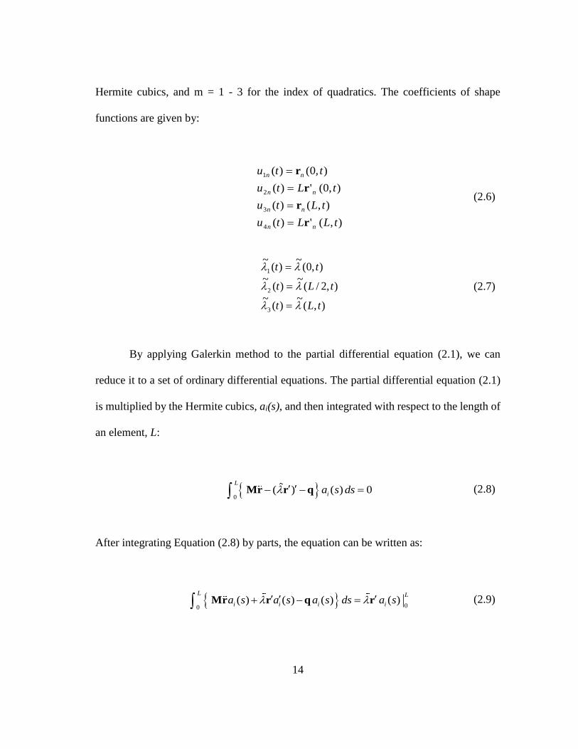
14
Hermite cubics, and m = 1 - 3 for the index of quadratics. The coefficients of shape
functions are given by:
),(')(
),()(
),0(')(
),0()(
4
3
2
1
tLLtu
tLtu
tLtu
ttu
nn
nn
nn
nn
r
r
r
r
(2.6)
),(~
)(~
),2/(~
)(~
),0(~
)(~
3
2
1
tLt
tLt
tt
(2.7)
By applying Galerkin method to the partial differential equation (2.1), we can
reduce it to a set of ordinary differential equations. The partial differential equation (2.1)
is multiplied by the Hermite cubics, ai(s), and then integrated with respect to the length of
an element, L:
0
( ) ( ) 0L
ia s ds Mr r q (2.8)
After integrating Equation (2.8) by parts, the equation can be written as:
00( ) ( ) ( ) ( )
L L
i i i ia s a s a s ds a s Mr r q r (2.9)

15
The right-hand side of the above equation represents the forces applied at the two ends of
an element which are named as generalized forces, fi.
0
1
2
3
4
(0) (0)
0
( ) ( )
0
L
i ia
L L
f r
f r F
f
f r F
f
(2.10)
We also obtain the constraint equation as follows:
2
0
1( ) (1 ) 1 0
2
L
mp s dsEA
r r (2.11)
Letting be / EA and plugging the expressions (2.3) into (2.9) and (2.11), we
can obtain the discretized forms of the ordinary differential equations (2.12) and the
constraint equations (2.13), respectively.
ikm njm kj ikm m kn im mn inM u u q f (2.12)
21 1 1
( 2 ) 02 2 2
ikm in kn iklm l l in kn mu u u u (2.13)
where, i, k = 1 – 4, and j, l, m = 1 – 3. It should be noted that inf is a tensor form of the
generalized forces. The coefficients in the equations are defined by:

16
1
0
1
0
1
0
1
0
1
0
1( ) ( ) ( )
( ) ( ) ( )
( ) ( )
( )
1( ) ( ) ( ) ( )
ikm i k m
ikm i k m
im i m
m m
iklm i k l m
a a p dL
L a a p d
L a p d
L p d
a a p p dL
(2.14)
Equation (2.12) involves twelve second-order ordinary differential equations, and
Equation (2.13) results in three algebraic equations. Let ( ) ( )K
inu t and ( ) ( )K
m t be values at
time step (K), then the updated values of inu and m at the next time step (K+1) are as
follows:
( 1) ( )
( 1) ( )
K K
in in in
K K
m m m
u u u
(2.15)
Substituting (2.15) into (2.12) and (2.13), and discarding the higher order terms,
the 15 equations for an element of the cable can be written in a matrix form, [A][ΔX]=[B].
The unknown vector, ΔX, is defined as follows:
11 12 13 21 22 23 1 2
31 32 33 41 42 43 3
( , , , , , , , ,
, , , , , , )T
u u u u u u
u u u u u u
X (2.16)

17
2.3. Boundary Conditions
In modeling a delta mooring system by FEM, four kinds of boundary conditions
are defined at four different locations namely, the fairleads, the smoothly connected
points, the joint of the three mooring segments, and the bottom as shown in Figure 4. At
the fairleads of mooring segments 1 and 2, hinged boundary conditions are applied. It
should be noted that the boundary conditions other than the hinge can be straightforwardly
extended. The support of the seabed is modeled as an elastic system.
Figure 4 Boundary Conditions of Delta Mooring System
2.3.1. Boundary Conditions at the Smooth Connections
Elements within each mooring segment in Figure 4 are smoothly connected at the
internal nodes if no concentrated external forces are applied. That is, the displacements
and gradients of the adjacent elements should be the same, while the internal tensions are

18
of the same value (but opposite directions). Therefore, the boundary conditions can be
expressed as:
( 1) ( )
3 1
( 1) ( 1) ( ) ( )
4 2
( 1) ( )
3 1
/ /
p p
n n
p p p p
n n
p p
u u
u L u L
(2.17)
where, (p-1) and (p) are indices of the neighboring elements, and (p-1) L and (p) L are the
length of (p-1) and (p) elements respectively. If there are no external forces and moments,
the generalized internal force should be balanced:
( 1) ( )
3 1 0p p
n nf f (2.18)
2.3.2. Boundary Conditions at the Jointed Connections
Similar to the boundary conditions at the smooth connection, the force at the joint
of the three segments should be balanced in the absence of concentrated external forces,
and the displacements at the jointed nodes of three neighboring elements have to be the
same. However, the gradients and the internal tensions of the elements at the jointed point
will not be the same. As shown in Figure 4, if elements (p), (q) and (r) are jointed, the
boundary conditions are:
( ) ( ) ( )
3 3 1
p q r
n n nu u u (2.19)

19
( ) ( ) ( )
3 3 1 0p q r
n n nf f f (2.20)
2.4. Formulation
The 15 unknowns of each element shown in equation (2.16) are governed by 15
equations. Since neighboring elements share 7 unknowns based on the boundary
conditions (2.17), the total unknowns for a cable can be reduced to 15+8(N-1) if a cable
has N elements without a delta joint. When the algebraic equations are summed up by
assembling procedure as shown in Figure 5, the summed generalized forces between
adjacent elements at the right-hand-side of equation, denoted by [B’], are cancelled out
owing to the force balancing condition (2.18). The prime denotes an assembled form of
[B]. Bandwidth of the coefficient matrix [A’] is 29.
For the case of a delta mooring line, the assembled matrix of each mooring segment
can be further manipulated using the boundary conditions (2.19). As a result, the total
unknowns for a delta mooring line can be reduced to 15+8(N1+N2+N3), where N1, N2 and
N3 are the numbers of elements for the three segments, respectively. Similar to the force
balancing condition for the case of smoothly connected elements, the boundary conditions
(2.20) are also satisfied in the right-hand side matrix [B’] of the assembled equations.
Figure 6 attempts to visualize how to assemble the matrix [A’] for the case of a
delta mooring line. For example, in this figure, the two hull-side (short) mooring segments
(A1 and A2) are divided into two elements (N1=N2=2), respectively. To assemble the
matrix of the three mooring segments, the coefficient matrix of the jointed elements among

20
mooring segments A1 and A2 should be rearranged in order to apply the boundary
condition (2.19). The unknown vectors for these last elements can be expressed as:
11 12 13 21 22 23 1 2
41 42 43 3 31 32 33
( , , , , , , , ,
, , , , , , )T
u u u u u u
u u u u u u
X (2.21)
In comparison with equation (2.16), the coefficients related to the displacements of the
joint node occupy the last three rows and the last three columns in the coefficient matrix
of the elements N1 and N2. Firstly, the mooring segments A2 and B form the assembled
matrix by sharing the displacements of the jointed node. Next, the last 3×3 diagonal part
in the matrix of the element N1 are later added to the overlapped parts (3×3) of the
previously assembled matrix, i.e., the purple box in Figure 6. The rest of the coefficients
in the last three rows and columns of the element N1’s matrix, i.e., the blue boxes in Figure
6, is rearranged by aligning with the overlapped part. The bandwidth depends on the
number of elements for the hull-side mooring segments (N2), and its values are 16N2+37.
Since the bandwidth of the systems of equations for a delta mooring line is larger than the
one for the single mooring line, it requires relatively high computational costs.

21
Figure 5 Assembled Matrix for a Cable with N Elements
Figure 6 Assembled Matrix for a Delta Mooring System
22
3. PRINCIPLES OF COUPLE-D-FAST
In this research, a numerical code called COUPLE-D-FAST is used to investigate
the FOWT dynamic responses. The code consists of two major modules, known as
COUPLE-D and FAST. Briefly, COUPLE-D calculates hydro-related forces, responses
of a delta mooring system, and 6 degrees of freedom (DOF) motions of a FOWT while
FAST computes wind-related forces and elastic forces of the tower and blades. The
overview of this code and some of the principles of modeling are described in following
subsections.
3.1. Modeling of FOWT in COUPLE-D
COUPLE (or COUPLE-D) was developed to analyze interactions between a
platform and its mooring lines or risers in time domain simulation which was and is being
developed by Prof. Jun Zhang and his former and current graduate students at Texas A&M
University and is written in FORTRAN (Cao and Zhang, 1997; Chen, 2002; Peng et al.,
2014; Min et al., 2016; Min and Zhang, 2017).
The Hywind FOWT system consists of a wind turbine, a floating platform moored
by a delta mooring system. When Hywind is modeled by COUPLE-D, the wind turbine
components are considered as rigid structures, i.e. the flexibility of the tower and blades
is not considered in COUPLE-D.
The 6 DOF nonlinear motion equations of a platform are coupled with the wind
external forces on the wind turbine governed by the aero-servo-elastic dynamic equations

23
and the dynamic equations of mooring lines through hinge boundary conditions. To solve
the motion equations in COUPLE-D, the Newmark-β method scheme is selected and
combined with iteration procedures to advance in time domain. The 6 DOF motion
equations can be summarized as (Paulling and Webster, 1986):
s a ( ) ( ) ( )x t x t x t M M B C F (3.1)
where, sM is the mass matrix of the FOWT system, aM is the added matrix, B the
damping matrix and C the restoring stiffness matrix. F denotes the summation of
external forces which include current forces, wave forces, mooring forces, aero-servo-
elastic forces, etc.
One of the dominant external forces acting on the floating structures is wave forces.
COUPLE-D-FAST has two options for calculating wave forces on the floating structure,
the second-order diffraction/radiation theory and the Morison equation using HWM.
A wave diffraction and radiation potential theory is the well-known method to
calculate wave forces, and one of the well-known numerical codes is WAMIT. In the
potential theory, the wave potential is solved numerically using a Boundary Element
Method in a frequency domain. Forces of this method consist of wave exciting forces,
added mass forces, and radiation damping forces. Wave drift damping forces could be
calculated by a heuristic formula (Aranha, 1994; Clark et al., 1993) without solving a
second-order low-forward speed diffraction and radiation problem. Then, all forces in

24
frequency domain are converted to forces in a time domain by the Inverse Fast Fourier
Transform (IFFT) or the convolution integral.
In this study, wave forces are calculated by the Morison equation instead of the
potential wave theory, since most FOWT platforms, like spar buoy, semi-submersible, and
tension leg platform, can be modelled as the combination of slender members.
For cylindrical structures, the Morison equation can be used to approximate wave
forces when the ratio of the typical wave length to the diameter is greater than 5 (λ>5D).
Accurate calculations of wave loads start with the accurate predictions of wave kinematics
because the calculation of the Morison equation requires wave kinematics of the ambient
fluid and the wave evolution. Wave kinematics could be calculated in many different
methods, like the second-order wave theory, the linear extrapolation, the Wheeler
stretching and the HWM. In this study, wave kinematics and wave elevations are
calculated using the HWM. Because HWM predicts nonlinear wave kinematics up to free
surface, the empirical stretching or approximations are not needed.
In using the HWM, an irregular wave spectrum is divided by three ranges: a very
low frequency range (pre-long wave band), a powerful range, and a very high frequency
region (restrictive band). The nonlinear effects wave components of a very low frequency
region are negligible because the amplitudes in the region are relatively small. The wave
components in the very high frequency region (restrictive band) are considered as the
bond-wave components instead of free-wave components.
The spectrum in the powerful range are further divided into three bands, a long
wave band and two of short wave bands as shown in Figure 7. The wave-wave interactions

25
within the same wave band are computed using the conventional perturbation approach.
The interactions between different wave bands are calculated using the phase modulation
approach. By applying the two different approaches, the solutions of wave kinematics
quickly converge for a wave field of a broad-banded spectrum.
Figure 7 Wave Frequency Band Division; Reprinted from Zhang et al. (1996)
3.2. Modeling of FOWT in FAST
In COUPLE-D-FAST, the aerodynamic forces are simulated by the AeroDyn
package in the FAST code. The FAST code is a nonlinear time domain simulator that uses
a combined modal- and multibody-dynamics formulation. FAST is able to simulate most
common wind turbine configurations and control scenarios (Jonkman, 2007). FAST
combines aerodynamics models (aero), hydrodynamic model for offshore wind turbine
(hydro), control and electrical system (servo), and structural dynamic models (elastic) to
simulate coupled nonlinear aero-hydro-servo-elastic computation in a time domain.

26
In FAST, the flexibility of the blades and tower is calculated using a linear modal
analysis. The nacelle and hub are considered as rigid bodies modelled by relevant lumped
mass and inertia terms. All DOFs can be controlled by switches which allows one to increase
or decrease the accuracy of the numerical model. The detailed explanation of the theoretical
background of FAST can be found in Jonkman (2007) and Moriarty and Hansen (2005).
3.2.1. Wake and Airfoil Modeling
The effects of aerodynamics for aero-elastic simulations of horizontal axis wind
turbine configurations are calculated using AeroDyn. It computes the aerodynamic lift, drag,
and pitching moment of airfoil sections along the wind turbine blades, which are determined
by dividing each blade into segments along the blade span. AeroDyn simultaneously collects
the geometry of turbine, operating condition, blade-element velocity and location, and wind
inflow. Those are employed to calculate the various forces for each segment, and then the
forces are used for calculating the distributed forces on the blades. The aerodynamic forces
have effect on turbine deflections and vice versa. AeroDyn takes advantage of relations based
on two dimensional localized flows, and the properties of the airfoils along the blade are
characterized by lift, drag, and pitching moment coefficients from results of wind tunnel
experiment. (Moriarty and Hansen, 2005)
3.2.2. Blade and Tower Flexibility
The flexibility of the blades and tower is considered using a linear modal analysis
with small deflections assumption for each member. The characteristics of the flexibility
for each member are decided by the distribution of mass and stiffness properties along the

27
span of the members, and by specifying their shapes as polynomials. In this research, the
functions of mode shapes are determined using BMODES which is a finite element code
to provide dynamically coupled modes for a beam and provided by NREL. In FAST,
blades behave in the directions of two flap-wise modes and an edgewise mode, and a tower
behave in the directions of two fore-after and two side-to-side modes. When generating
blade modes, the rotor speed will affect significantly the frequency of vibration while it
slightly affects the mode shapes (Jonkman, 2007).
3.2.3. Control System
For the NREL 5 MW baseline wind turbine, two control systems are employed for
a stability of a generator of the wind turbine: a generator-torque controller and a blade-
pitch controller. The two control systems are modeled to operate individually in the below-
rated and above-rated wind speed range, respectively. The generator-torque control system
is intended for maximizing the power capture below the rated operation condition. The
blade-pitch control system is intended for regulating the generator speed above the rated
operation condition. (Jonkman et al., 2009)
3.3. Coupling Overview of COUPLE-FAST
In COUPLE-D-FAST, FAST is used to calculate the wind forces, the servo
dynamic forces of a wind turbine, and the effects of flexible materials. On the other hand,
COUPLE-D computes the mooring forces of a delta mooring system and the

28
hydrodynamic forces on the FOWT platform using HWM; as a result, COUPLE-D
calculates the global motions of the FOWT platform using the forces estimated by FAST.
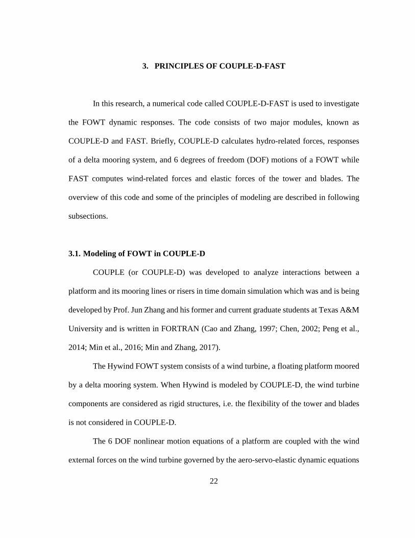
In terms of the components of a structure, the major difference among COUPLE-
D and FAST is the flexibilities of a tower and blades of a wind turbine. Both programs
consider the bodies of a platform as rigid structures, but FAST considers the tower and
blades as flexible parts, which differs from that COUPLE-D assumes the whole parts of
FOWT are rigid. Therefore, the appropriate correction for the differences is required for
coupling the independent programs. FAST computes the forces at the bottom of the turbine
tower which include wind forces and servo dynamic forces as well as inertial forces with
flexibility. Meanwhile, COUPLE-D calculates the inertial forces above the bottom of the
tower using the rigid-body assumption. The differences of the forces between FAST and
COUPLE-D are calculated, and then directly used for the analysis of global motions of
FOWT in COUPLE-D. The coupling procedure is described in Figure 8, and more details
of the coupling procedure will be presented in following subsections.
The time step of the COUPLE-D module can be determined relating to that of
FAST. The time step of COUPLE-D can be the same as that of FAST or larger than that
because the motions of the tower (FAST) have large natural frequency compared to the
motions of the supporting platform (COUPLE-D), and the forces acting on the floating
platform (COUPLE-D) varies relatively slowly with respect to the forces on
rotor/nacelle/tower (FAST). By applying a relatively large time step in COUPLE-D, the
CPU time can decrease substantially (Peng, 2015). In this study, the time steps are 0.01
sec in the FAST module and 0.05 sec in the COUPLE-D module.
29
Figure 8 Flowchart of Coupling Procedure of COUPLE-D-FAST
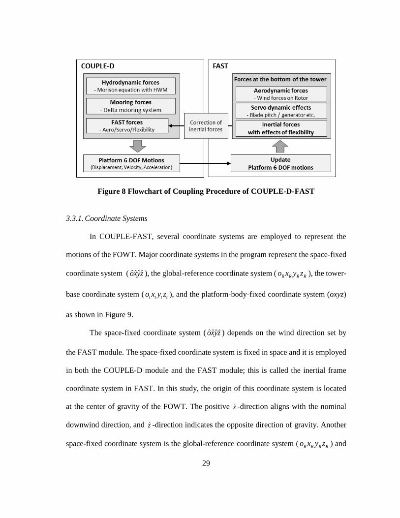
3.3.1. Coordinate Systems
In COUPLE-FAST, several coordinate systems are employed to represent the
motions of the FOWT. Major coordinate systems in the program represent the space-fixed
coordinate system ( ˆ ˆˆˆoxyz ), the global-reference coordinate system ( R R R Ro x y z ), the tower-
base coordinate system ( t t t to x y z ), and the platform-body-fixed coordinate system (oxyz)
as shown in Figure 9.
The space-fixed coordinate system ( ˆ ˆˆˆoxyz ) depends on the wind direction set by
the FAST module. The space-fixed coordinate system is fixed in space and it is employed
in both the COUPLE-D module and the FAST module; this is called the inertial frame
coordinate system in FAST. In this study, the origin of this coordinate system is located
at the center of gravity of the FOWT. The positive x -direction aligns with the nominal
downwind direction, and z -direction indicates the opposite direction of gravity. Another
space-fixed coordinate system is the global-reference coordinate system ( R R R Ro x y z ) and

30
is also fixed in space. The directions of winds, waves, currents, and mooring lines, can be
defined by this coordinate system. As shown in Figure 10, its xR and yR axes are defined
with respect to the angle of wind direction in the space-fixed coordinate system. The z-
axis of this coordinate system coincides with that of the space-fixed coordinate system.
Figure 9 Coordinate Systems of Hywind in COUPLE-D-FAST
31
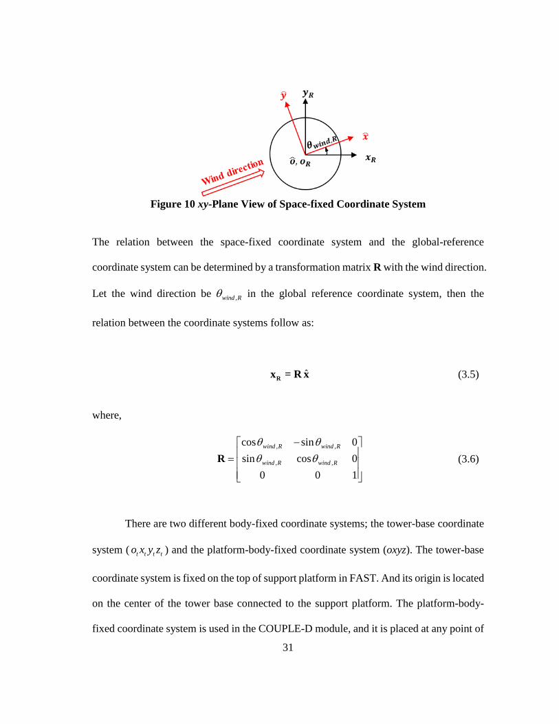
Figure 10 xy-Plane View of Space-fixed Coordinate System
The relation between the space-fixed coordinate system and the global-reference
coordinate system can be determined by a transformation matrix R with the wind direction.
Let the wind direction be ,wind R in the global reference coordinate system, then the
relation between the coordinate systems follow as:
ˆR
x = R x (3.5)
where,
, ,
, ,
cos sin 0
sin cos 0
0 0 1
wind R wind R
wind R wind R
R (3.6)
There are two different body-fixed coordinate systems; the tower-base coordinate
system ( t t t to x y z ) and the platform-body-fixed coordinate system (oxyz). The tower-base
coordinate system is fixed on the top of support platform in FAST. And its origin is located
on the center of the tower base connected to the support platform. The platform-body-
fixed coordinate system is used in the COUPLE-D module, and it is placed at any point of

32
the platform or the center of gravity. In this study, its origin point is located at the center
of gravity of the FOWT. This coordinate system overlaps exactly with ˆ ˆˆˆoxyz when the
platform is at its initial position. The two body-fixed coordinate systems move and rotate
with the platform motion as shown in Figure 11.
Figure 11 Body-fixed Coordinate Systems
The relation between the space-fixed coordinate system and the platform-body-
fixed coordinate system is defined by a transformation matrix T with Euler angles. When
the platform is moved with the translational motion, and is rotated with the Euler angles,
the relation between x in oxyz and x in ˆ ˆˆˆoxyz can be expressed as:
ˆ tx = ξ + T x (3.7)
where,

33
3 2 3 1 3 2 1 3 1 3 2 1
3 2 3 1 3 2 1 3 1 3 2 1
2 2 1 2 1
cos cos sin cos cos sin sin sin sin cos sin cos
sin cos cos cos sin sin sin cos sin sin sin cos
sin cos sin cos cos
T
(3.8)
where, ξ is the translational motion, and 1 , 2 , and 3 represent the angle of roll, pitch,
and yaw in ˆ ˆˆˆoxyz , respectively.
3.3.2. Mathematical Formulation of Coupling Problem
a. Static coupling problem
For the initial time step, COUPLE-D calculates the mean position by computing
mean current and wave drifting forces acting on the platform and mooring lines’ and
hydrostatic restoring forces. This is initial position of the platform used in FAST. This
static equation for the FOWT is expressed as:
( ) mean HSn Mx t C F F F (3.9)
where, meanF is mean forces applied on the platform of the FOWT, HSnF is nonlinear
restoring forces, and MF is mooring system forces.
b. Dynamic coupling problem
The motion equations (3.1) can be modified as following expression under the
Morison approach.
34
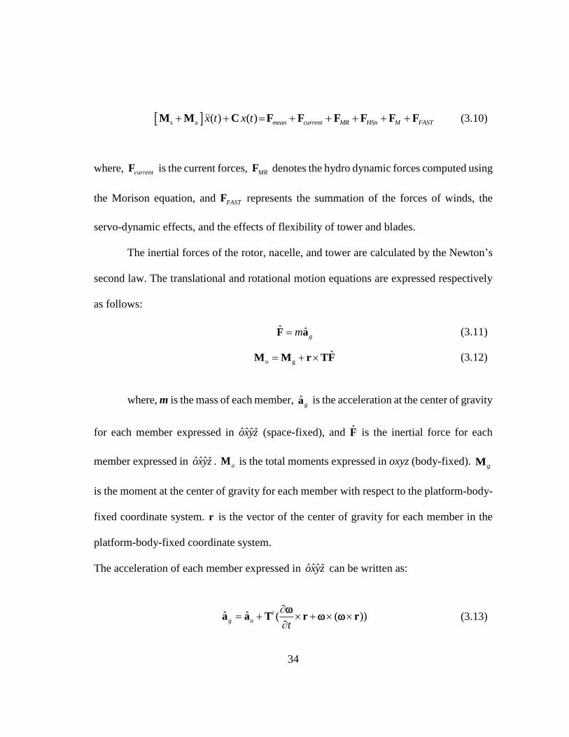
s a ( ) ( ) mean current MR HSn M FASTx t x t M M C F F F F F F (3.10)
where, Fcurrent is the current forces, FMR denotes the hydro dynamic forces computed using
the Morison equation, and FFAST represents the summation of the forces of winds, the
servo-dynamic effects, and the effects of flexibility of tower and blades.
The inertial forces of the rotor, nacelle, and tower are calculated by the Newton’s
second law. The translational and rotational motion equations are expressed respectively
as follows:
ˆ ˆgmF a (3.11)
o g
ˆ M M r TF (3.12)
where, m is the mass of each member, ag is the acceleration at the center of gravity
for each member expressed in ˆ ˆˆˆoxyz (space-fixed), and F is the inertial force for each
member expressed in ˆ ˆˆˆoxyz . oM is the total moments expressed in oxyz (body-fixed). gM
is the moment at the center of gravity for each member with respect to the platform-body-
fixed coordinate system. r is the vector of the center of gravity for each member in the
platform-body-fixed coordinate system.
The acceleration of each member expressed in ˆ ˆˆˆoxyz can be written as:
ˆ ˆ ( ( ))t
g ot
a a T r r
(3.13)

35
where, ˆoa is the acceleration of the platform at the origin expressed in ˆ ˆˆˆoxyz , and is the
angular velocity expressed in oxyz.
FAST returns the wind forces, the servo-dynamic effects, and the inertial forces
above the bottom of the tower expressed in t t t to x y z . The force vector FFAST can be written
as:
, , ,
ˆ ˆ ˆ )
( )
T F (F F FF
M r F M M M
t
t R N T
FAST
t TB t g R g N g T
(3.14)
where, tF and tM given by FAST are the forces and moments at the bottom of the tower
expressed in t t t to x y z , respectively. TBr is the vector of the bottom of the tower expressed
in oxyz. FR , FN and FT represent the inertial forces of the rotor, nacelle, and tower which
are calculated by COUPLE-D and expressed in ˆ ˆˆˆoxyz , respectively. ,Mg R
, ,Mg N
and
,Mg T are the inertial moments of the rotor, nacelle, and tower which are calculated by
COUPLE-D and expressed in oxyz, respectively.
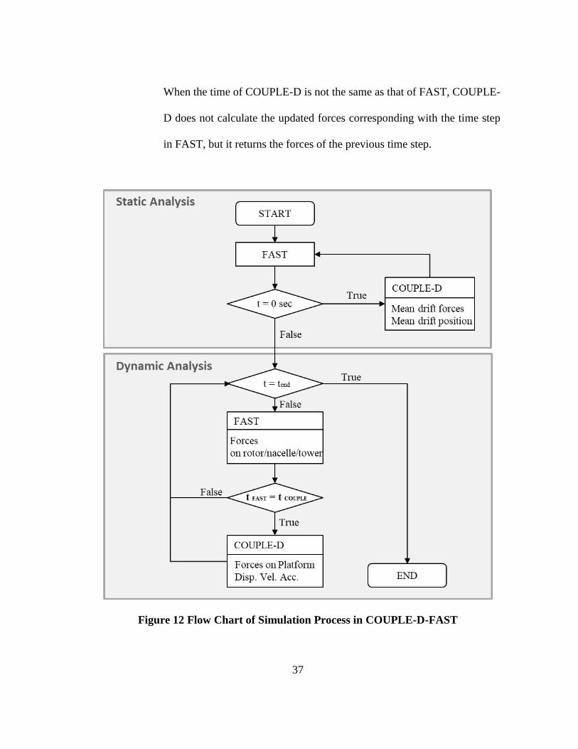
3.3.3. Coupling Procedures of COUPLE-D-FAST
Since the time steps of the FAST and COUPLE-D modules are 0.01 sec and 0.05
sec, respectively in the program, COUPLE-D is only activated every five time steps of
FAST. The coupling procedure is summarized as follows, and the flow chart is plotted in
Figure 12.

36
1. Initial Position (t = 0 sec); Static Analysis
1) COUPLE-D determines the mean position by the mean current and wave
drifting forces on the platform, ant it transfers the position and forces into
FAST.
2) FAST sets the initial position of the FOWT using the position from
COUPLE-D.
2. Time Marching Stage; Dynamic Analysis (t > 0 sec, and tFAST = tCOUPLE)
1) FAST collects all forces applied on the rotor/nacelle/tower with respect to
the tower-base coordinate system, and it transports the forces to COUPLE-
D.
2) COUPLE-D calculates all forces acting on the platform, but excluding the
aerodynamic portions. It also computes inertial forces of the
rotor/nacelle/tower under the condition that COUPLE-D does not allow a
deflection of each member. COUPLE-D subtracts the inertial forces from
the forces given by FAST. As a result, the differences, equation (3.14),
among the two kinds of forces represent the wind forces on the rotor, the
servo-dynamic effects and the effects of flexibility of the tower and blades.
3) Then, COUPLE-D predicts motions, velocities, and accelerations of the
FOWT using all external forces including the differences from 2).
4) Finally, COUPLE-D provides the predicted displacements, velocities,
accelerations, and external forces for FAST.
3. Time marching stage (t > 0 sec, but tFAST ≠ tCOUPLE)
37
When the time of COUPLE-D is not the same as that of FAST, COUPLE-
D does not calculate the updated forces corresponding with the time step
in FAST, but it returns the forces of the previous time step.
Figure 12 Flow Chart of Simulation Process in COUPLE-D-FAST

38
4. NUMERICAL MODEL SET-UP AND CALIBRATION
The 5 MW Hywind FOWT was employed for the model test and hence for the
numerical simulations in this research. In the following subsections, the experimental
facilities and set-up of the model are briefly described, and additionally, the calibration
for certain parameters, such as the hydrodynamic coefficients and wind turbine tower
stiffness used in the numerical simulations, is also described.
4.1. Model Experiments
4.1.1. Experimental Facilities
The behaviors of the Hywind FOWT under aerodynamic and wave loads were
tested and measured in the Deepwater Offshore Basin in SJTU (Duan et al., 2015). The
wave basin had the following dimensions 50 m (length) × 40 m (width) × 10 m (depth),
and the waves and currents were achieved by a 222 multi-independence flap wave
generator. The facility was able to produce quality wind fields using its generation system,
which was designed and modified for the model tests. The wind generation system used
nine axial fans to produce parallel wind fields. Its output dimensions were 3.76 m × 3.76
m and it had a capacity of up to 9.53 m/s. A honeycomb-shaped screen was placed in front
of the wind fans to generate a steady wind-quality wind flow and to lower turbulence
intensity.

39
4.1.2. Set-up of Model and Instruments
The prototype FOWT was geometrically scaled down following a 1:50 Froude
similitude. The properties of the 5 MW NREL reference wind turbine (Jonkman et al.,
2009) and floating system from the OC3 project (Jonkman, 2010) were used in the model
test. The mooring system’s properties and water depth followed the MARIN’s experiment
(Koo et al., 2012).
In the experiments, the properties of the wind turbine model were modified to be
equipped with measuring instruments such as motion sensors and load cells. The mass
properties of the SJTU’s Hywind model were then compared with those of the prototype
and the MARIN’s model tests (see Table 1). It should be noted that the mass and length
values listed refer to the prototype unless otherwise specified, and the center of mass
represents the distance from the mean water level. The blades in the model test were made
from woven carbon fiber epoxy composite materials due to limitations in mass scaling
resulting from the Froude similitude. Thus, they could only be approximated as rigid,
inflexible blades. The tilt angles of the shaft and blade pre-cone were 0 degrees, and blade
pitch control was not allowed.
The spar-buoy platform of Hywind was also modified to match the mass and center
of gravity of the total system by adjusting the metal ballast. The platform’s main
characteristics are listed in Table 2. The moment of inertia in yaw was not measured in
the SJTU’s model test. Thus, in this research the yaw moment of inertia was estimated by
its counterpart in the MARIN’s experiment (Koo et al., 2012). It was determined to be 100

40
× 106 kg-m2 based on the mass ratio of the SJTU’s platform to the MARIN’s platform.
Figure 13 shows the installed FOWT model and the spar platform.
In the model tests, several measuring devices were installed, including an
accelerometer, optical motion sensor, two load cells, and three tension sensors (as shown
in Figure 14). One load cell was placed between the nacelle and tower, and the other was
located at the rear part of the nacelle. The load cells were able to capture loads in three
translational and three rotational directions. The accelerometer (3 DOF) was installed at
the nacelle, and the optical motion sensor (6 DOF) was located at the bottom of the turbine
tower. A taut delta mooring system with a 200 m water depth was employed in the SJTU’s
model test, which was accomplished by the MARIN’s model test (Koo et al., 2012). Its
layout and the locations of the tension sensors are depicted in Figure 14 (a). The properties
of the delta mooring system are listed in Table 3.
(a) (b)
Figure 13 Model Setting (a) and Floating Platform (b); Reprinted from Duan et al.
(2015)

41
Table 1 Mass Properties of Hywind Model (Duan et al., 2015)
Property Unit NREL* MARIN** SJTU***
Blades kg 53,220 48,750 52,659
Hub kg 56,780 72,880 57,272
Nacelle kg 240,000 274,900 239,082
Tower mass kg 249,718 164,600 287,128
Instruments on tower kg - 137,640 113,391
Platform mass kg 7,466,330 7,281,600 7,316,578
Total system mass kg 8,066,048 7,980,370 8,066,110
Total system center m -78.00 -76.35 -78.95
* Jonkman and Musial (2010);** Koo et al. (2012);***Duan et al. (2015)
Table 2 Platform Properties of Hywind Model
Property Unit NREL* MARIN** SJTU***
Overall length m 130 130 130
Draft m 120 120 120
Platform center of mass m -89.92 -91.1 -94.15
Platform mass kg 7,466,330 7,281,600 7,316,578
Platform Roll Inertia kg·m² 4,229,230,000 3,966,000,000 4,656,382,813
Platform Pitch Inertia kg·m² 4,229,230,000 3,966,000,000 4,656,382,813
Platform Yaw Inertia kg·m² 164,230,000 98,600,000 Not measured
* Jonkman and Musial (2010);** Koo et al. (2012);***Duan et al. (2015)
(a) (b)
Figure 14 Mooring Layout (a) and Assembled Devices (b); (b) is reprinted from
Duan et al. (2015)
42
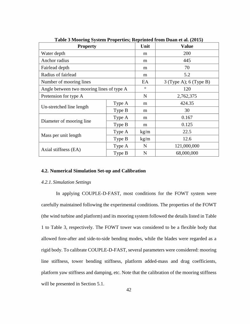
Table 3 Mooring System Properties; Reprinted from Duan et al. (2015)
Property Unit Value
Water depth m 200
Anchor radius m 445
Fairlead depth m 70
Radius of fairlead m 5.2
Number of mooring lines EA 3 (Type A); 6 (Type B)
Angle between two mooring lines of type A ° 120
Pretension for type A N 2,762,375
Un-stretched line length Type A m 424.35
Type B m 30
Diameter of mooring line Type A m 0.167
Type B m 0.125
Mass per unit length Type A kg/m 22.5
Type B kg/m 12.6
Axial stiffness (EA) Type A N 121,000,000
Type B N 68,000,000
4.2. Numerical Simulation Set-up and Calibration
4.2.1. Simulation Settings
In applying COUPLE-D-FAST, most conditions for the FOWT system were
carefully maintained following the experimental conditions. The properties of the FOWT
(the wind turbine and platform) and its mooring system followed the details listed in Table
1 to Table 3, respectively. The FOWT tower was considered to be a flexible body that
allowed fore-after and side-to-side bending modes, while the blades were regarded as a
rigid body. To calibrate COUPLE-D-FAST, several parameters were considered: mooring
line stiffness, tower bending stiffness, platform added-mass and drag coefficients,
platform yaw stiffness and damping, etc. Note that the calibration of the mooring stiffness
will be presented in Section 5.1.

43
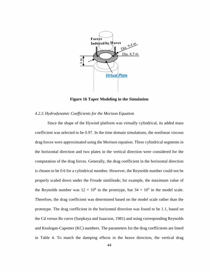
4.2.2. Hywind Platform Model
The platform shape of Hywind can be divided into three sections. The platform
diameter above the taper of the platform was 6.5 m, and the diameter below the taper was
9.4 m. In this study, the platform was simplified as a combination of three cylinders with
different diameters (as shown in Figure 15). In short, the taper section was simplified as a
cylinder with a 7.95 m diameter, which is the diameter of the taper’s midsection. The
vertical forces acting on the taper section were estimated from the forces acting on a virtual
plate located at the taper’s midsection as shown in Figure 16. It should be noted that the
vertical forces were applied only on the side of the plate faced up.
(a) Geometry in the model test
(b) Geometry in the simulation
Figure 15 Geometry of Hywind Spar
44
Figure 16 Taper Modeling in the Simulation
4.2.3. Hydrodynamic Coefficients for the Morison Equation
Since the shape of the Hywind platform was virtually cylindrical, its added mass
coefficient was selected to be 0.97. In the time domain simulations, the nonlinear viscous
drag forces were approximated using the Morison equation. Three cylindrical segments in
the horizontal direction and two plates in the vertical direction were considered for the
computation of the drag forces. Generally, the drag coefficient in the horizontal direction
is chosen to be 0.6 for a cylindrical member. However, the Reynolds number could not be
properly scaled down under the Froude similitude; for example, the maximum value of
the Reynolds number was 12 × 106 in the prototype, but 34 × 103 in the model scale.
Therefore, the drag coefficient was determined based on the model scale rather than the
prototype. The drag coefficient in the horizontal direction was found to be 1.1, based on
the Cd versus Re curve (Sarpkaya and Isaacson, 1981) and using corresponding Reynolds
and Keulegan-Capenter (KC) numbers. The parameters for the drag coefficients are listed
in Table 4. To match the damping effects in the heave direction, the vertical drag

45
coefficients of the taper section and bottom of the platform were chosen to be 0.35 and
3.0, respectively.
Table 4 Parameters for Estimation of Drag Coefficient
Wave
Height
(m)
Wave
Period
(sec)
Water
Particle
Velocity
Amplitude
(m/s)
Diameter
at surface
(m)
KC
number
Reynolds number
Model Prototype
2 8 0.79 6.5 0.97 14×103 5×10⁶
4 10 1.26 6.5 1.93 23×103 8×10⁶
7.1 12.1 1.84 6.5 3.43 34×103 12×106
4.2.4. Tower Stiffness Tests
The properties of the wind turbine tower used in the model test were different from
those of the reference tower mentioned in the OC3 project, due to the measuring
instruments installed in the tests. This led to different shapes and mass distributions
compared to those of the OC3’s reference tower. The tower used in the experiments was
built from aluminum tubes with different diameters. The tower properties in the simulation
needed to be calibrated to simulate the tower behavior. In the simulation, the tower was
considered to be comprised of six cylindrical tubes with different diameters, and the
tower’s mass and center of gravity corresponded to the values used in the experiment.
The forces induced by the tower’s flexibility were calculated via the linear modal
analysis in the FAST module. The mode shapes for the fore-after and side-to-side were
calculated using BMODES provided by NREL. The multiplier of the tower stiffness was
considered to match the first fore-after mode frequencies for both the model test and

46
simulation. Then, the first mode frequencies were computed using a Fast Fourier
Transform (FFT) of the accelerations of the nacelle; the values were 0.46 Hz in the model
test and 0.47 Hz in the simulation.
4.3. Fixed Wind Turbine Test
Since the Hywind prototype was geometrically scaled down according to a Froude
scale in the experiment, the viscous wind forces from winds could not be appropriately
reproduced. If the wind speeds followed the Froude scale in the model test, the wind forces
on the rotor of the wind turbine would be too small. Therefore, the discrepancy between
the model and the prototype needed to be properly treated.
In the model tests, Duan et al. (2015) adjusted the wind speeds to obtain the
targeted rotor thrust. The targeted rotor thrust was initially calculated by the FAST
simulations under the conditions that the wind turbines were fixed to the ground as if they
were the on-land wind turbines, and the blade pitch controller was operated with changes
in wind speeds. It should be noted that the wind speeds in the FAST simulation were
defined as “nominal,” which was different from the wind speeds in the model tests. The
wind turbine in the model test was also mounted on a fixed base, and the wind speeds were
adjusted to meet the targeted thrust forces. For cases of wind speeds exceeding 11.4 m/s
(the rated wind speed), the testing wind speeds were lowered below the nominal wind
speeds. This was because the blades were fixed on the hub in the model test, whereas the
blades’ pitch angles in the FAST simulation were adjusted by the blade pitch controller.
Table 5 shows a comparison of the results from the model tests with those of the FAST

47
simulations. The table shows that the measured mean thrust forces matched the thrust force
predicted by FAST, but the related rotor speeds did not match.
Table 5 Fixed Wind Turbine Test Results; Reprinted from Duan et al. (2015)
Wind speed (m/s) Thrust (kN) Rotor speed (rpm)
FAST Model FAST Model FAST Model
5.0 9.4 276 276 7.5 7.9
11.4 12.8 770.4 770.4 12.1 14.4
18.0 11.1 451.1 451.1 12.1 10.9

48
5. INVESTIGATION OF HYWIND RESPONSES1
In this section, the capacities of COUPLE-D-FAST are examined through
comparisons with the related results obtained, respectively, using COUPLE-FAST and
FAST-OrcaFlex, and the measurements at the SJTU’s wave basin. It should be noted that
the reference point of the FOWT’s global motion in the SJTU’s tests was located at the
mean water level before external forces were applied. To verify the mooring model in
COUPLE-D-FAST, static offset tests were implemented to validate the mooring stiffness.
The properties of Hywind, such as natural periods and damping effects, were then
determined based on free-decay tests. Finally, the Hywind’s global motion was
investigated through wind-only load cases.
5.1. Mooring Stiffness Test
To verify the mooring model in COUPLE-D-FAST, the mooring forces from
COUPLE-D-FAST were compared with those of COUPLE-FAST and FAST-OrcaFlex,
and the SJTU’s measurements. A simplified mooring system was used in COUPLE-FAST.
However, the delta mooring system was employed for the other simulations. A multibody
formulation was used to simulate the delta mooring system in FAST-OrcaFlex (i.e., each
jointed node was altered by a massless buoy). Figure 17 shows the mooring layouts in the
1 Part of this section is reprinted with permission from "Numerical Simulation of a Floating Offshore Wind
Turbine Constrained by Delta Mooring System" by Min and Zhang (2017). Proceedings of the 27th (2017)
International Offshore and Polar Engineering Conference, Copyright [2017] by the International Society of
Offshore and Polar Engineers (ISOPE)

49
numerical simulations using the three different codes. Comparisons were made for the
static offset tests and the shapes of the mooring lines.
(a) COUPLE-FAST (b) COUPLE-D-FAST (c) FAST-OrcaFlex
Figure 17 Mooring Layouts in the Simulations
The horizontal offset tests were conducted within a surge or sway range of 0 to 6
m for the model tests, and within 0 to 10 m for the simulations. The results of the static
offset tests from the model test and numerical simulations are plotted in Figure 18. Figure
18(a) and (b) show that the simulated stiffness curves for the surge and sway directions,
respectively, agree well with the measurements. It should be noted that the available
experimental results for the static offset test were limited only in the surge and sway
directions. All simulated results for the heave direction were in good agreement, as shown
in Figure 18(c). Because differences among the simulations were very small, they are
indistinguishable in these figures. The yaw rotational offset test was implemented within
a range of 0 to 10 degrees to examine the delta mooring model’s yaw-stiffness capacity as

50
compared to the single mooring model. The yaw stiffness curve comparisons show very
good agreement between the predictions by COUPLE-D-FAST and FAST-OrcaFlex (see
Figure 18(d)). This clearly demonstrates that the developed mooring code in COUPLE-D-
FAST properly captured the mooring forces of the delta mooring system. Moreover, it also
shows that the delta mooring system significantly increased the yaw-restoring moments,
as compared to the case of a simplified mooring system, although the effect of the delta
mooring system was insignificant in the translational directions.
(a) Surge
(b) Sway
(c) heave
(d) Yaw
Figure 18 Static Offset Test Comparisons; (a) and (d) are reprinted with
permission from Min and Zhang (2017)

51
Figure 19 depicts the mooring line configuration when the yaw angle was 10
degrees. The mooring lines’ segments were almost identically shaped for both COUPLE-
D-FAST and FAST-OrcaFlex, but COUPLE-FAST showed a different profile due to the
simplification of the mooring system. This clearly indicates that the delta mooring system
can substantially increase yaw stiffness, which is consistent with the comparison
illustrated in Figure 18(d). This supports the superiority of the explicit simulation of delta
mooring system, and also shows that it provides more realistic mooring behaviors.
Figure 19 Configuration of Mooring Lines (Yaw=10°); Reprinted with permission
from Min and Zhang (2017)

52
5.2. Free-decay Tests
5.2.1. Free-decay Tests without Tuned Parameters
Free-decay tests were carried out to determine the properties of Hywind such as
natural periods and damping effects. The free-decay results are shown in Figure 20 and
Figure 21 for the translational and rotational directions, respectively. It should be noted
that additional tunings for better matching were not included in these Figures.
Overall, the simulated free-decay for surge, sway, and heave were in good
agreement with the measurements, as shown in Figure 20. The surge motions of the
floating structure were closely related to the restoring forces of its mooring system. Figure
20(a) indicates that the simulated results of all of the numerical models were in satisfactory
agreement with the model test results, suggesting that the numerical codes were able to
accurately simulate the restoring effects of the mooring system. In the heave free-decay
tests, COUPLE-FAST and COUPLE-D-FAST rendered similar responses with the
experiments, as shown in Figure 20(c), while FAST-OrcaFlex showed a slightly different
natural period.
Figure 21 illustrates the free-decay results for rotational directions. In the roll and
pitch decay tests plotted in Figure 21(a) and (b), respectively, the simulated natural periods
rendered much smaller values than the measured ones. The reason for this phenomenon
has not yet been identified. Additional tunings might be needed to match the decay results
for the model test and simulations. The pitch decay test comparison indicated that Hywind
was slightly under-damped compared to the model test after 50 sec. This may be because
the installed cables in the model test (as shown in Figure 13) could have created a damping

53
effect on the FOWT system. In Figure 21(c), the yaw decay simulations considering the
delta mooring system – COUPLE-D-FAST and FAST-OrcaFlex – were in excellent
agreement with the experiment, but the simulated natural periods were slightly smaller
than the measurement. This might be because the estimated yaw moment of inertia was
slightly smaller than in the model test. It should be noted that he yaw moment of inertia
was not measured in the model test. The yaw decay results from COUPLE-FAST clearly
show that the natural period and damping effects could not be captured properly without
explicit modeling. The following section describes the tunings of the platform properties
that were made to obtain better agreement in the free-decay tests.
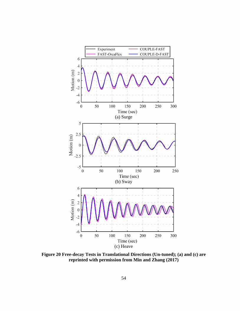
54
(a) Surge
(b) Sway
(c) Heave
Figure 20 Free-decay Tests in Translational Directions (Un-tuned); (a) and (c) are
reprinted with permission from Min and Zhang (2017)
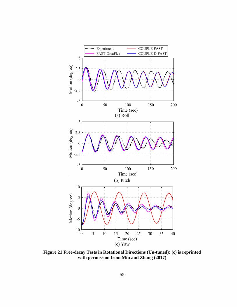
55
(a) Roll
.
(b) Pitch
(c) Yaw
Figure 21 Free-decay Tests in Rotational Directions (Un-tuned); (c) is reprinted
with permission from Min and Zhang (2017)

56
5.2.2. Free-decay Tests with Adjusted Parameters
The platform properties were adjusted based on a better agreement between the
simulation results and the related rotational free-decay tests. The moments of inertia were
adjusted by increasing 26% and 14% of the moments of inertia in the FOWT system’s roll
and pitch, respectively. For all simulations, the yaw moment of inertia for the Hywind
platform was increased by 10%. The additional yaw damping and stiffness were set to 22
× 106 N-m/(rad/s) and 108 × 106 N-m/(rad), respectively, only for the COUPLE-FAST
simulation. To include the cables’ effects at the wind turbine tower, we considered a linear
damper with a magnitude of 14 (kN/m/s), which was attached at the mid-section of the
tower. The adjusted parameters are listed in Table 6.
Table 6 Adjusted Parameters of the FOWT System
Simulation
model
Roll Pitch Yaw
Additional
Moment of
Inertia
kg-m2
Additional
Moment of
Inertia
kg-m2
Additional
Moment of
Inertia
kg-m2
Additional
Damping
N-m/(rad/s)
Additional
Stiffness
N-m/rad
FAST-OrcaFlex 91×108 49×108 10×106 - -
COUPLE-FAST 91×108 49×108 10×106 22×106 108×106
COUPLE-D-FAST 91×108 49×108 10×106 - -
Figure 22 shows the results of the free-decay tests for the rotational directions.
Because the adjusted properties hardly affected the translational motion, the related figures

57
(surge, sway, and heave) were omitted for brevity. Using the adjusted parameters listed in
Table 6, the simulated decays were in good agreement with the related measurement. In
Figure 22(c), the measured and simulated yaw motions agreed well, but the FAST-
OrcaFlex simulation showed relatively low damping effects while the COUPLE-D-FAST
showed good agreement with the measurements. A comparison of the simulated and
measured natural periods can be found in Table 7. Although the yaw natural period
computed by COUPLE-FAST showed better agreement with the measurements than those
obtained using the other codes, all predicted yaw natural periods were insignificantly
different from the various models considered (within 0.2 sec).
Table 7 Natural Period of Hywind FOWT; Reprinted with permission from Min
and Zhang (2017)
Case Surge Heave Pitch Yaw
Experiment 40.46 27.60 33.94 5.95
FAST-OrcaFlex 40.72 28.22 32.88 6.12
COUPLE-FAST 40.83 27.78 33.66 6.00
COUPLE-D-FAST 40.76 27.78 33.78 6.08
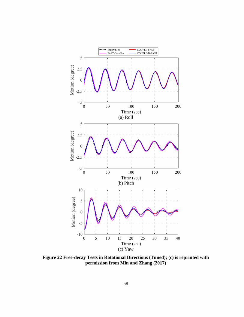
58
(a) Roll
(b) Pitch
(c) Yaw
Figure 22 Free-decay Tests in Rotational Directions (Tuned); (c) is reprinted with
permission from Min and Zhang (2017)

59
5.3. Corrections of Wind Speeds
Due to a misunderstanding of the coordinate system for the wind thrust between
the experiment and the FAST simulation, the wind speeds in the model test based on the
fixed wind turbine test in Table 5 were overestimated and need to be corrected
accordingly. In the experimental setting, the rotor shaft axis was parallel to the horizontal
direction of the global coordinate system (as shown in Figure 23(a)). Therefore, the
measured thrust forces were caused solely by the wind thrust. However, as shown in
Figure 23(b), the shaft in the FAST simulation was tilted by -5 degrees, which is the
default setting of the NREL’s 5MW reference wind turbine (Jonkman et al., 2009). This
indicates that the simulated thrust forces included a portion of the rotor weight, in addition
to the wind thrust. The rotor weight’s portion of the thrust force was approximately 94 kN
(= 9.81 × 109.9 × sin(5°)) in the simulation. For example, in the case of 5 m/s winds (see
Table 5), the measured wind force was 51% larger than the simulated wind force.
(a) Experiment (b) Simulation
Figure 23 Initial Settings of Rotor in SJTU’s Study; Reprinted with permission
from Min and Zhang (2017)

60
When the simulation used the nominal wind speed given by Duan et al. (2015), the
overestimated wind conditions led to a significant discrepancy in the motion of the FOWT
between the model test and the simulation, specifically in the mean surge and pitch
motions (Min et al., 2016). Therefore, the nominal wind speeds needed to be corrected
based upon the settings used in the experiment, instead of the default setting (as in the
NREL case). Hence, the shaft tilt and pre-cone angles were explicitly set to be 0 degrees
in running FAST, consistent with the settings for the model test. With the corrected
settings, the nominal wind speeds were redefined to proper values through the FAST
simulations. Since the blade pitch control was not included in the experiment, the control
system was also not included in the FAST simulation. Without the pitch controller, the
blade pitch angles in the simulation were chosen to be the angles corresponding with the
selected wind speeds. Table 8 shows a comparison of the results from the model tests with
those of the FAST simulations. The simulated thrust forces under the corrected wind
speeds were well matched with the corresponding measurements. The first two wind
conditions in Table 8 are named Operational conditions 1 and 2, and the final wind
condition is called the Extreme condition in this research.
Table 8 Redefined Wind Speed; Reprinted with permission from Min and Zhang
(2017)
Wind speed (m/s) Rotor thrust (kN) Rotor speed (rpm) Blade pitch (°)
FAST Model FAST Model FAST Model FAST Model
I 6.55 9.4 275.3 276 8.24 7.9 0 0
II 14.30 11.1 451.0 451.1 12.10 10.9 9.28 0
III 11.41 12.8 770.0 770.4 12.57 14.4 0 0
I: Operational condition 1; II: Operational condition 2; III: Extreme condition

61
5.4. Motions of Hywind under Steady Wind Loads
To investigate the effects of wind loads on Hywind, three different nominal wind
speeds of 6.55 (Operational 1), 14.30 (Operational 2) and 11.41 (Extreme) m/s at the hub
height were used in the numerical simulations using COUPLE-FAST, COUPLE-D-FAST,
and FAST-OrcaFlex for one-half hour. The average platform motion and mooring tension
for the upstream (U) and downstream (D) sides were compared with the measurements in
Table 9. Under steady winds, the dynamic motions and forces were very small, so their
comparisons were omitted. It should be noted that the FOWT’s average surge and heave
motions were at the mean water level. The average motions and forces from the COUPLE-
FAST and COUPLE-D-FAST simulations rendered very similar responses, indicating that
the delta mooring system had less impact on the FOWT’s motions, except with yaw
motions. However, the direct modeling of the delta mooring system has an advantage in
that additional tuning of the yaw stiffness and damping was not needed. Interestingly, the
FAST-OrcaFlex simulation showed slightly larger discrepancies in the platform motions
in comparison with the other two simulations. This discrepancy may have resulted from
differences in the modeling approach.
Even though corrected wind speeds were used in the simulations, the predicted
pitch motions were still smaller than the measured values, as indicated in Table 9.
However, it should be noted that they were greatly improved compared to the results of
our previous study (Min et al., 2016), as listed in Table 10. Figure 24 offers a visual
comparison of the results obtained from the previous results of Min et al. (2016), the
present results from COUPLE-D-FAST and FAST-OrcaFlex, and the model test.
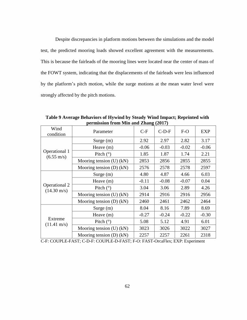
62
Despite discrepancies in platform motions between the simulations and the model
test, the predicted mooring loads showed excellent agreement with the measurements.
This is because the fairleads of the mooring lines were located near the center of mass of
the FOWT system, indicating that the displacements of the fairleads were less influenced
by the platform’s pitch motion, while the surge motions at the mean water level were
strongly affected by the pitch motions.
Table 9 Average Behaviors of Hywind by Steady Wind Impact; Reprinted with
permission from Min and Zhang (2017)
Wind
condition Parameter C-F C-D-F F-O EXP
Operational 1
(6.55 m/s)
Surge (m) 2.92 2.97 2.82 3.17
Heave (m) -0.06 -0.03 -0.02 -0.06
Pitch (°) 1.85 1.87 1.74 2.21
Mooring tension (U) (kN) 2853 2856 2855 2855
Mooring tension (D) (kN) 2576 2578 2578 2597
Operational 2
(14.30 m/s)
Surge (m) 4.80 4.87 4.66 6.03
Heave (m) -0.11 -0.08 -0.07 0.04
Pitch (°) 3.04 3.06 2.89 4.26
Mooring tension (U) (kN) 2914 2916 2916 2956
Mooring tension (D) (kN) 2460 2461 2462 2464
Extreme
(11.41 m/s)
Surge (m) 8.04 8.16 7.89 8.69
Heave (m) -0.27 -0.24 -0.22 -0.30
Pitch (°) 5.08 5.12 4.91 6.01
Mooring tension (U) (kN) 3023 3026 3022 3027
Mooring tension (D) (kN) 2257 2257 2261 2318
C-F: COUPLE-FAST; C-D-F: COUPLE-D-FAST; F-O: FAST-OrcaFlex; EXP: Experiment

63
Table 10 Average Behaviors of Hywind by Steady Wind Impact; Reprinted from
Min et al. (2016)
Parameter
Wind condition
Operational 1
(5 m/s)
Operational 2
(18.0 m/s)
Extreme
(11.4 m/s)
Surge (m) 1.88 3.78 7.47
Heave (m) -0.01 -0.04 -0.20
Pitch (°) 1.19 2.40 4.73
Mooring tension (U) (kN) 2822 2883 3003
Mooring tension (D) (kN) 2644 2527 2297
Figure 24 Average Platform Motions and Mooring Tensions

64
5.5. Discussion
In this section, COUPLE-D-FAST’s capability for modeling the delta mooring
system was examined through static offset and free-decay tests, and steady wind impact-
only tests. Corrections of wind speeds were made prior to simulating the wind impact-
only cases, because the tested wind speeds were initially overestimated as mentioned in
Section 5.3. The delta mooring system was directly modeled in COUPLE-D-FAST and
FAST-OrcaFlex, while COUPLE-FAST used a simplified model for the mooring system.
The model test and all simulations were in satisfactory agreement with regards to mooring
stiffness in surge and sway. In terms of yaw stiffness, COUPLE-D-FAST and FAST-
OrcaFlex showed similar mooring stiffness values that were much greater than those
predicted by COUPLE-FAST.
In the yaw decay tests, the motions obtained using COUPLE-D-FAST and FAST-
OrcaFlex showed good agreement with the related measurements, indicating the
superiority of direct modeling of the delta mooring system. In terms of roll and pitch,
however, the simulated natural periods were smaller than the measured ones. This led to
case-specific increases in the moments of inertia in those directions, so that the computed
free-decay motions agreed well with the measurements. However, the increases (26% in
roll and 14% in pitch) might not be negligible tuning but be regarded as unrealistic tuning.
In addition, the simulated mean motions rendered smaller values than the measurements,
even though the wind speeds were corrected in Section 5.3. The discrepancies of the free-
decay tests and the mean FOWT motions are further investigated in the next section.
65
6. INVESTIGATION OF HYWIND RESPONSES WITH CORRECTED
CENTER OF GRAVITY
Although the corrected wind speeds were used in COUPLE-D-FAST and FAST-
OrcaFlex (see Section 5.4), the improvements were not enough to yield satisfactory
agreement with the related measurements of the global motions. To understand the source
or reasons for the discrepancies between the simulations and related measurements, we
firstly focused on the comparison of the mean global motion of the FOWT. The simulated
results from COUPLE-D-FAST are compared with those of the SJTU’s model test under
various environmental conditions.
Eleven cases were used in the comparison include wind impact-only, irregular
wave impact-only, wind with regular waves, and wind with irregular waves. The
comparisons involve global platform motions and mooring tensions in both time and
frequency domains. Prior to applying the various met-ocean conditions, the FOWT’s
center of gravity was corrected through simulations using measured wind forces, and free-
decay tests were then implemented to examine the effects of this correction.
6.1. Environmental Conditions
6.1.1. Turbulent Wind Conditions
While the application of steady wind conditions was described in Section 5.3,
turbulent wind conditions were applied at this stage of the research to make the simulated
winds more similar to those used in the model tests. Similar to the results given in Section

66
5.3, the redefined nominal wind speeds based on the fixed wind turbine tests but under the
impact of the turbulence winds are given in Table 11. While the nominal wind speeds of
Operational 1 and Extreme conditions remain the same as compared to the corresponding
wind speeds in Section 5.3, the wind speeds of Operational condition 2 were lowered to
keep the consistency of the model test condition that the blade pitch rotation was not
allowed.
Because the time series of wind speeds from the model tests were not available,
the turbulence intensities for Operational 1, Operational 2, and Extreme conditions were
chosen to be 5%, 3%, and 2%, respectively, and the turbulent winds for the simulations
were generated using the TurbSim program (Jonkman, 2009). The turbulence intensities
were selected based on the spectral analysis for surge and pitch motions under the wind
load only conditions. Figures 25 to 27 show comparisons of surge and pitch spectrum
obtained using COUPLE-D-FAST under the steady and turbulent wind conditions and the
model test. As shown in these figures, the simulated surge and pitch under turbulence wind
conditions show good agreement with the corresponding measurements while dynamic
responses are barely observable in the simulations under steady wind conditions.
Table 11 Wind Speeds
Wind speed (m/s) Rotor thrust (kN) Rotor speed (rpm) Blade angle (°)
FAST Model FAST Model FAST Model FAST Model
I 6.55 9.4 275.6 276 8.2 7.9 0 0
II 8.62 11.1 451.3 451.1 9.9 10.9 0 0
III 11.41 12.8 770.2 770.4 12.6 14.4 0 0
I: Operational condition 1; II: Operational condition 2; III: Extreme condition

67
(a) Surge (b) Pitch
Figure 25 Comparison of Surge and Pitch Amplitude Spectrum (Operational 1)
(a) Surge (b) Pitch
Figure 26 Comparison of Surge and Pitch Amplitude Spectrum (Operational 2)
(a) Surge (b) Pitch
Figure 27 Comparison of Surge and Pitch Amplitude Spectrum (Extreme)
6.1.2. Met-ocean Conditions
Eleven different cases were simulated in this study. They can be divided into four
sets: wind load-only (LC01-LC03), wave load-only (LC04 and LC05), combined wind
and regular wave loads (LC06-LC08), and combined wind and irregular wave loads

68
(LC09-LC11). The Joint North Sea Wave Project (JONSWAP) spectrum was employed
to generate irregular waves in both the model test and simulation. The wave conditions in
LC05, LC10, and LC11 represented one year return period in the Gulf of Maine (Koo et
al., 2012). To prevent sudden “jerk” movements of the FOWT at the beginning, a 100
seconds sine-function ramp function was applied on the simulated external forces at the
beginning. The met-ocean conditions for all of the cases are summarized in Table 12.
Table 12 Environmental Conditions
CASE Wind speeds (m/s)
Waves Model Simulation
Wind
only
LC01 9.4 6.55 -
LC02 11.1 8.62 -
LC03 12.8 11.41 -
Irregular
waves only
LC04 - - 2 m / 8 sec (γ = 3.3)
LC05 - - 7.1 m / 12.1 sec (γ = 2.2)
Winds +
Regular
waves
LC06 9.4 6.55 2 m / 8 sec
LC07 11.1 8.62 6 m / 11 sec
LC08 12.8 11.41 4 m / 10 sec
Winds +
Irregular
waves
LC09 9.4 6.55 2 m / 8 sec (γ = 3.3)
LC10 11.1 8.62 7.1 m / 12.1 sec (γ = 2.2)
LC11 12.8 11.41 7.1 m / 12.1 sec (γ = 2.2)
6.2. Correction of the Center of Gravity
6.2.1. Simulation using Measured Wind Forces
After the corrections to the nominal wind speeds were made, the simulated average
surge and pitch are still smaller than the corresponding measurements listed in Section
5.4. To investigate these discrepancies, we conducted simulations directly using the
measured wind loads instead of using FAST’s predictions.

69
The measurements at Load Cell #1 (see Figure 14(b)) were chosen instead of those
of Load Cell #2 because the mass property of the motor in the nacelle was not specified
in the model test. Considering that Load Cell #1 was moving and rotating with respect to
the FOWT’s movement, the loads should have been transformed to the reference frame:
ˆ ˆˆˆoxyz (space-fixed) for translational directions and oxyz (body-fixed) for rotational
directions. Since the measured wind load is directly applied in the simulation (instead of
the FAST computation), the motion equation (Eq. 3.10) is written as:
s a ( ) ( ) M M C F F F F F Fmean current MR HSn M EXPx t x t (4.1)
ˆ
ˆ( )
T F FF
M r F TF
t
measured TOP
EXP
measured TOP measured TOP
(4.2)
where, FEXP is the measured wind forces at Load Cell #1 after the exclusion of inertia
force and moment, FTOP represents the inertial forces above Load Cell #1 in ˆ ˆˆˆoxyz ,
Fmeasured and Mmeasured are the measured forces and moments, respectively, at Load Cell #1,
and rTOP is the location of Load Cell #1 in the oxyz coordinates. The mass above Load Cell
#1 was estimated to be 449.013 tons, which included the upper parts of the wind turbine
tower. Then, the weight effects induced by the pitch motions were subtracted from the
measured forces. Nine cases were simulated using this approach, and the results are listed
in Table 13. Figure 28 shows the average surge and pitch motions predicted using this
approach and their comparisons with the measured values. Overall, the predicted average

70
surge and pitch are still smaller than the corresponding measurements. The under-
predictions of mean surge may be likely caused by the smaller average pitch, because the
mean surge is compared at the mean water level, not at the center of gravity of the system.
Table 13 Environmental Conditions for Simulations using Measured Wind Forces
Wind
condition
Mean wind forces
at the load cell #1
(in model test)
Wave condition
Type H // T or Hs // Tp
Operational 1
281.5 kN - -
282.3 kN Regular waves 2 m // 8 sec
268.3 kN Irregular waves 2 m // 8 sec
Operational 2
506.8 kN - -
481.5 kN Regular waves 6 m // 11 sec
445.1 kN Irregular waves 7.1 m // 12.1 sec
Extreme
757.2 kN - -
685.1 kN Regular waves 4 m // 10 sec
698.0 kN Irregular waves 7.1 m // 12.1 sec
(a) Surge (b) Pitch
Figure 28 Average Platform Motions using Measured Wind Forces

71
6.2.2. Correction of the Center of Gravity
Wind forces are one of the dominant factors affecting the mean surge and pitch of
the FOWT. After measured wind forces were used as input in the simulation, we attempted
to find which other factors were responsible for the smaller predicted average pitch. The
other important factors determining mean surge and pitch include the FOWT system’s
mooring line restoring force and hydrostatic stiffness. Because the surge stiffness from the
model test and the simulation were in relatively satisfactory agreement (as shown in Figure
18(a)), the main reason for the small pitch motions is likely caused by the hydrostatic
stiffness, which was dominated by the distance between the centers of buoyancy (CB) and
the center of gravity (CG) of the FOWT.
In the experiment, the spar platform’s CG could be inaccurate because there were
uncertainties such as the location of the metal ballast in the spar and the spar’s complicated
inner space. This led to a reconsideration of the location of the FOWT’s CG, which is
closely related to the pitch stiffness of the floating system. The CG for the total system
was estimated to be -76.267 m, while the CG given by the model test was -78.947 m.
The pitch moment of inertia and the FOWT system’s stiffness were re-estimated
based on the corrected CG, and they were then compared to the corresponding calculations
based on the given CG as listed in Table 14. As shown in this table, the stiffness by
hydrostatic and mooring system decreased largely (-16%) after applying the correction of
CG although the change regarding the pitch moment of inertia was relatively insignificant
(-4%). It should be noted that the additional tunings for the pitch moment of inertia are
not included in this estimation. Figure 29 shows pitch free-decay comparisons of two
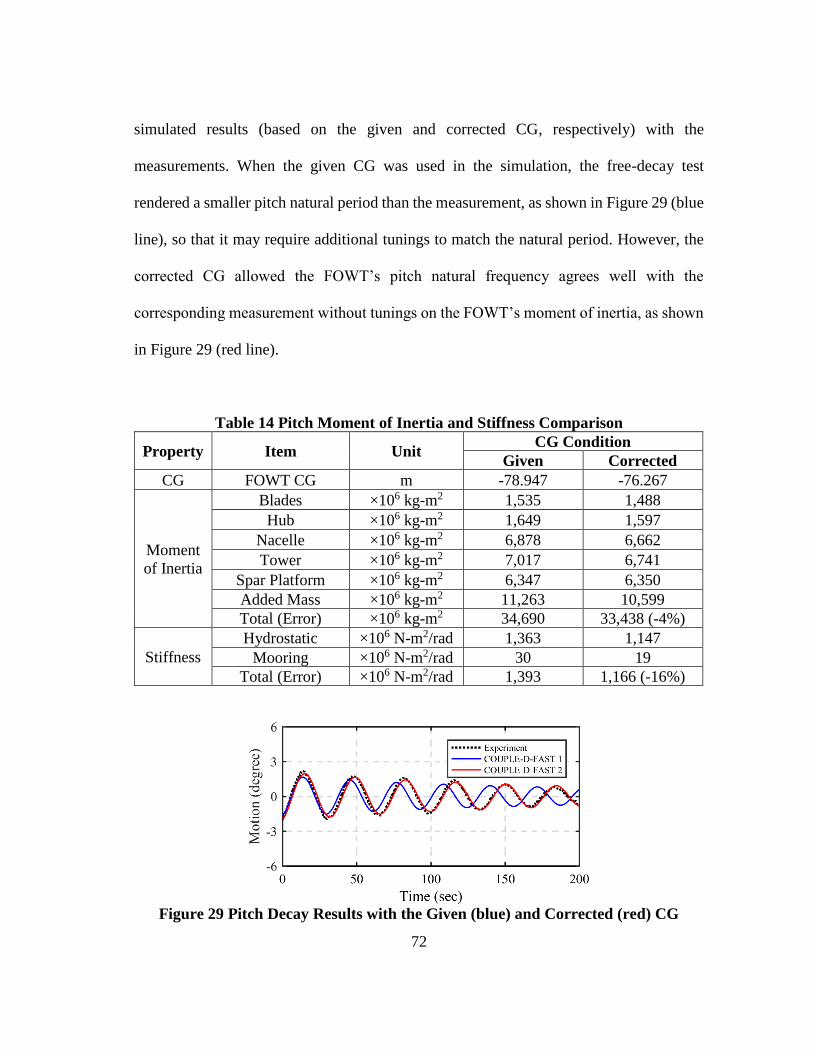
72
simulated results (based on the given and corrected CG, respectively) with the
measurements. When the given CG was used in the simulation, the free-decay test
rendered a smaller pitch natural period than the measurement, as shown in Figure 29 (blue
line), so that it may require additional tunings to match the natural period. However, the
corrected CG allowed the FOWT’s pitch natural frequency agrees well with the
corresponding measurement without tunings on the FOWT’s moment of inertia, as shown
in Figure 29 (red line).
Table 14 Pitch Moment of Inertia and Stiffness Comparison
Property Item Unit CG Condition
Given Corrected
CG FOWT CG m -78.947 -76.267
Moment
of Inertia
Blades ×106 kg-m2 1,535 1,488
Hub ×106 kg-m2 1,649 1,597
Nacelle ×106 kg-m2 6,878 6,662
Tower ×106 kg-m2 7,017 6,741
Spar Platform ×106 kg-m2 6,347 6,350
Added Mass ×106 kg-m2 11,263 10,599
Total (Error) ×106 kg-m2 34,690 33,438 (-4%)
Stiffness
Hydrostatic ×106 N-m2/rad 1,363 1,147
Mooring ×106 N-m2/rad 30 19
Total (Error) ×106 N-m2/rad 1,393 1,166 (-16%)
Figure 29 Pitch Decay Results with the Given (blue) and Corrected (red) CG
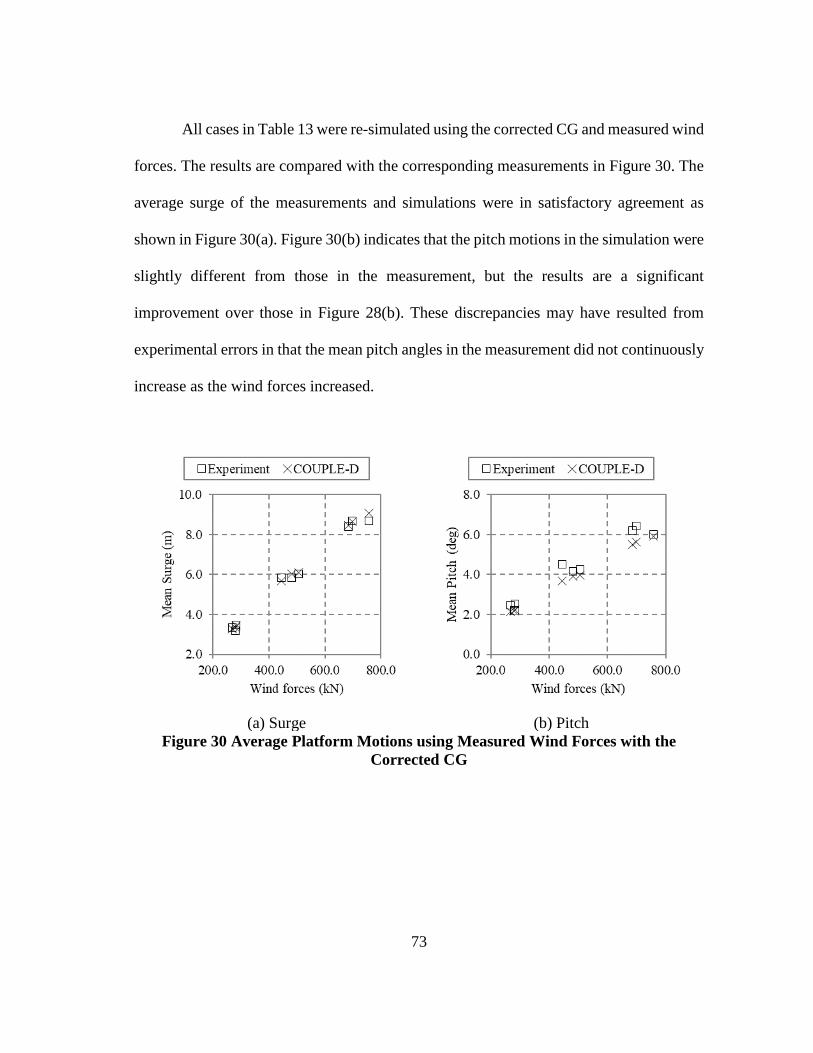
73
All cases in Table 13 were re-simulated using the corrected CG and measured wind
forces. The results are compared with the corresponding measurements in Figure 30. The
average surge of the measurements and simulations were in satisfactory agreement as
shown in Figure 30(a). Figure 30(b) indicates that the pitch motions in the simulation were
slightly different from those in the measurement, but the results are a significant
improvement over those in Figure 28(b). These discrepancies may have resulted from
experimental errors in that the mean pitch angles in the measurement did not continuously
increase as the wind forces increased.
(a) Surge (b) Pitch
Figure 30 Average Platform Motions using Measured Wind Forces with the
Corrected CG

74
6.3. Free-decay Tests
The corrected center of gravity could have changed the Hywind’s natural
frequency because it results in a change in the hydrostatic stiffness. With the corrected
center of gravity, the Hywind’s natural periods and damping were investigated again
through the related free-decay tests.
Since the change to the center of gravity hardly affected the free-decay of the
translational motion, the related free-decay comparisons have been omitted for brevity.
Additional fine tuning was done to produce better agreement between the simulation and
model tests. The tuned parameters are listed in Table 15. In the roll decay test, the roll
moments of inertia were increased by 10% over the total roll moments of inertia in the
simulations. A linear damper with a magnitude of 14 (kN/m/s) was considered so as to
include the cables’ effects at the mid-point of the wind turbine tower. Figure 31 shows the
results of the free-decay tests for rotational directions. As shown in this figure, the free-
decay simulations were in satisfactory agreement with the measurement although a small
surge natural period in FAST-OrcaFlex was rendered. The simulated and measured natural
periods are compared in Table 16.
Table 15 Additional Tuning of the FOWT System
Case
Roll Pitch Yaw
Additional
Moment of
Inertia
kg-m2
Additional
Moment of
Inertia
kg-m2
Additional
Moment of
Inertia
kg-m2
Additional
Damping
N-m/(rad/s)
Additional
Stiffness
N-m/rad
FAST-OrcaFlex 33×108 - 10×106 - -
COUPLE-FAST 33×108 - 10×106 22×106 108×106
COUPLE-D-FAST 33×108 - 10×106 - -
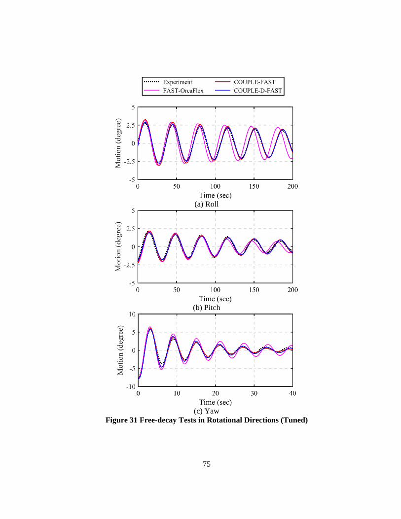
75
(a) Roll
(b) Pitch
(c) Yaw
Figure 31 Free-decay Tests in Rotational Directions (Tuned)

76
Table 16 Natural Period of the Hywind System (Unit: sec)
Case Surge Sway Heave Roll Pitch Yaw
Experiment 40.46 40.94 27.60 35.60 33.94 5.95
FAST-OrcaFlex 40.73 40.85 28.12 34.40 32.98 6.12
COUPLE-FAST 40.77 40.80 27.78 35.49 33.80 6.00
COUPLE-D-FAST 40.74 40.80 27.78 35.49 33.88 6.08
The simulated and measured mooring tensions at the two fairleads and joints of
each mooring line were also compared. The layout of the mooring system and mooring
line index numbers are given in Figure 32. For the yaw decay test, Figure 33 and Figure
34 show comparisons of the downstream- and upstream-side mooring line tensions for
COUPLE-D-FAST and FAST-OrcaFlex, respectively. Note that the mooring line tensions
were not recorded in the measurements for free-decay tests. Figure 33(a) and (b) include
a comparison of the mooring tensions at the fairleads on the downstream-side (Tensions
3-1 and 3-2), which could not be computed when a simplified mooring system was used
such as in the COUPLE-FAST simulation. Both the COUPLE-D-FAST and FAST-
OrcaFlex simulations rendered very similar responses. With regards to the tensions at the
delta mooring joint, while the simulated results showed similar responses in the initial
stage (0 to 10 seconds) during the yaw decay test, they rendered somewhat different
oscillations after that stage. For the upstream side illustrated in Figure 34, the overall
simulated results from both numerical models were in satisfactory agreement at the
fairleads tensions, but some differences were observed in the case of the tensions at the
delta joint (as shown in Figure 34(c)) after 10 seconds at the downstream-side mooring
line.

77
Figure 32 Mooring Layout for Indexing

78
(a) Tension 3-1 (Fairlead)
(b) Tension 3-2 (Fairlead)
(c) Tension 3 (Delta joint)
Figure 33 Downstream-side Mooring Tension during Yaw Free-decay

79
(a) Tension 2-1 (Fairlead)
(b) Tension 2-2 (Fairlead)
(c) Tension 2 (Delta joint)
Figure 34 Upstream-side Mooring Tension during Yaw Free-decay

80
6.4. CASE I: Turbulent Winds Impact-Only Cases
Three turbulent wind conditions corresponding to the cases of Operational 1
(LC01), Operational 2 (LC02), and Extreme (LC03) were simulated for a one-hour
duration using COUPLE-D-FAST. Figure 35 lists the comparisons of the average platform
motion and mooring line tension at joints for the measurement, previous (Min and Zhang,
2017), and current simulations. The numerical comparisons are listed in Table 17. It
should be noted that the CG given by the model test was employed in the Min and Zhang
(2017)’s simulations. In Figure 35, it is shown that the mean positions from the current
simulations were much improved over those in Min and Zhang (2017), indicating that the
CG was properly corrected. For LC01 and LC03, the simulated results were in good
agreement with the measurements. However, some discrepancies in the mean surge were
observed in LC01 and LC03, while the mean pitch motions in the simulations agreed well
with the measurements. It should also be noted that the differences of mean surge between
the simulated results of COUPLE-D-FAST and the measurements were relatively small,
approximately 4 and 10 mm in the model scale for LC01 and LC03, respectively.
LC02 evidenced simulated surge and pitch motions that were smaller than the
measurement. This could have been because the measured wind forces were larger than
the simulated forces. Although the surge and pitch motions for the model test and
simulation were somewhat different for LC02, the mooring line tensions for the
simulations and model test were in excellent agreement. This is because the displacements
at the fairleads (-70 m from the mean water level) were not as large as the platform
displacements at the mean water level.

81
Figure 35 Average Platform Motions and Mooring Tensions (LC01-LC03)

82
Table 17 Averages of Platform Motions and Mooring Tensions (LC01-LC03)
CASE Parameter C-D-F (Old)1 C-D-F2 EXP3
LC01
Surge (m) 2.97 3.37 3.17
Heave (m) -0.03 -0.04 -0.06
Pitch (°) 1.87 2.21 2.21
Mooring tension 1 (kN) 2855.8 2852.4 2855.1
Mooring tension 2 (kN) 2855.4 2856.6 2854.6
Mooring tension 3 (kN) 2578.2 2582.3 2596.8
LC02
Surge (m) 4.87 5.50 6.03
Heave (m) -0.08 -0.10 0.04
Pitch (°) 3.06 3.60 4.26
Mooring tension 1 (kN) 2916.1 2911.5 2956
Mooring tension 2 (kN) 2916.7 2918.2 2949.6
Mooring tension 3 (kN) 2461.1 2468.5 2463.5
LC03
Surge (m) 8.16 9.19 8.69
Heave (m) -0.24 -0.29 -0.30
Pitch (°) 5.12 6.02 6.01
Mooring tension 1 (kN) 3025.5 3018.9 3026.6
Mooring tension 2 (kN) 3021.1 3027.1 3010.7
Mooring tension 3 (kN) 2256.9 2272.2 2317.5 1 Min and Zhang (2017)’s COUPLE-D-FAST results 2 COUPLE-D-FAST 3 Experiment

83
6.5. CASE II: Waves Impact-Only Cases
6.5.1. Wave Generation
The JONSWAP spectrum was employed to generate irregular waves in both the
model test and simulations. Two irregular wave conditions were generated in this study.
In the first, the irregular waves had a significant wave height of 2 m and a peak period of
8 sec, with a shape factor of 3.3 (LC04); in the other, the waves had a significant wave
height of 7.1 m and a peak period of 12.1 sec, with a shape factor of 2.2 (LC05). To
reproduce the waves from the model tests in the simulation, we used the phase information
obtained from the resultant waves of the model tests by using IFFT. However, with regards
to the wave amplitudes, the values obtained using the JONSWAP spectrum were used. In
the simulation, the nonlinear effects of wave-wave interactions were predicted by HWM.
Figure 36 and Figure 37 include comparisons of the measured and simulated wave
elevations for LC05 in time and frequency domains, respectively. Overall, the computed
wave elevations agreed with the measurements well, as shown in Figure 36. The amplitude
spectra of the measurement and simulation were also in good agreement in both the wave
frequency (WF) range (0.05 < f < 0.20 Hz) and the low frequency (LF) range (f < 0.05
Hz), as shown in Figure 37. This clearly indicates that the nonlinear effects of wave-wave
interactions were well-predicted by the HWM. However, in the WF range, the amplitude
at the peak frequency of the measurement is slightly larger than the simulated one.

84
Figure 36 Wave Elevations (LC05)
Figure 37 Spectrum of Wave Elevations (LC05)

85
6.5.2. Simulation Results
The case of LC04 has a significant wave height of 2 m and a peak period of 8 sec.
The statistics of the FOWT’s motions and mooring tensions are listed in Table 18. Figure
38 shows the comparisons between the measured time series and amplitude spectra for the
surge, heave, pitch, and yaw motions and the corresponding predictions. The amplitude
spectra were obtained using Fast Fourier Transform (FFT) and an 8-point average
smoothing window. Figure 38(a) shows that the average heave motions in the simulation
were approximately zero while the measured motions shifted to the positive z-axis
direction. This may have been caused by inaccuracy in the measurements because the
shifted heave was relatively small (about 3 mm in the model scale). With regard to the
platform’s dynamic motions within the WF range, 0.05 to 0.20 Hz, Figure 38(b) showed
satisfactory agreement between the experiment and the simulation, except for the yaw
dynamic motions. While the measurements showed some yaw dynamic motions, the
simulated yaw motions were barely observable. Near the surge natural frequency, the
surge responses predicted using COUPLE-D-FAST were slightly smaller than those of the
experiment.
To examine the discrepancies in heave and yaw motions, the simulated motions
from COUPLE-D-FAST were also compared with the corresponding results predicted
using FAST-OrcaFlex. Figure 39 shows the platform’s heave and yaw motions obtained
respectively using the two different programs were in satisfactory agreement. It should be
noted that the platform yaw motions were barely observable in both simulations. Imperfect

86
axisymmetric settings for the wave direction and/or mooring layout may have caused these
yaw motions in the measurements.
Table 18 Statistics for Platform Motions and Mooring Tensions (LC04)
Mean SD Max Min
Surge (m) Experiment 0.068 0.611 -0.454 0.167
Simulation 0.012 0.548 -0.523 0.155
Heave (m) Experiment 0.200 0.383 0.085 0.042
Simulation 0.002 0.102 -0.076 0.030
Pitch (°) Experiment 0.151 0.516 -0.224 0.097
Simulation 0.006 0.367 -0.299 0.080
Yaw (°) Experiment -0.106 0.093 0.260 -0.442
Simulation 0.000 0.000 0.000 0.000
Tension 1
(kN)
Experiment 2775.2 2830.1 2732.4 13.4
Simulation 2763.1 2802.5 2731.5 10.7
Tension 2
(kN)
Experiment 2781.2 2873.7 2691.3 28.7
Simulation 2763.1 2802.5 2731.5 10.7
Tension 3
(kN)
Experiment 2768.9 2868.9 2672.8 33.5
Simulation 2761.5 2828.0 2691.2 21.0
Figure 40 offers a comparison of the mooring line tensions between the
measurements and simulations. The measured and simulated mooring tensions were in
good agreement, as shown in Figure 40(a). The tension spectra for the downstream side
(Mooring Line 3) showed good agreement while the spectra for the upstream side
(Mooring Lines 1 and 2) did not (see Figure 40(b)). Specifically, the tensions in Mooring
Line 1 was much smaller than those in Mooring Line 2. Ideally, the mooring tensions in
the upstream lines should show similar responses because the upstream mooring line
layout were symmetric with respect to the wave propagation direction. These
discrepancies are also observed in Figure 40(b). The significant differences between
tension amplitude spectra of Lines 1 and 2 near the surge natural frequency may have been
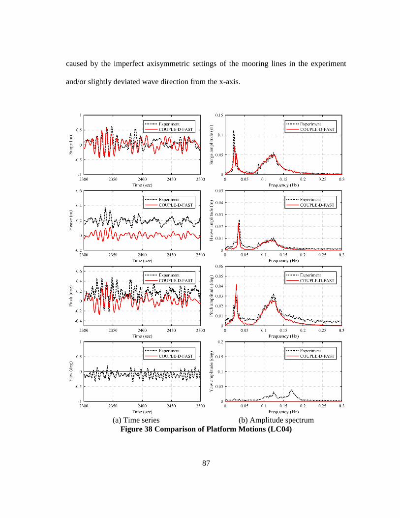
87
caused by the imperfect axisymmetric settings of the mooring lines in the experiment
and/or slightly deviated wave direction from the x-axis.
(a) Time series (b) Amplitude spectrum
Figure 38 Comparison of Platform Motions (LC04)
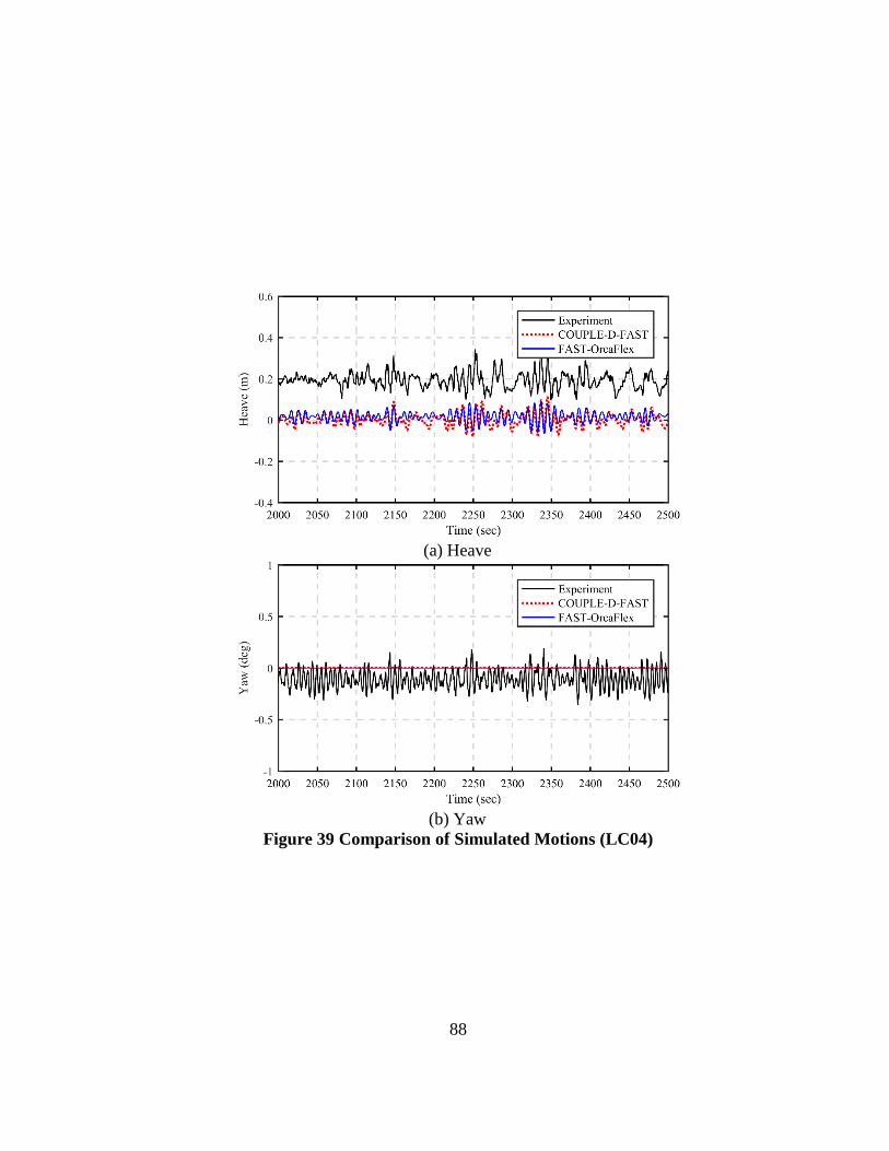
88
(a) Heave
(b) Yaw
Figure 39 Comparison of Simulated Motions (LC04)

89
(a) Time series (b) Amplitude spectrum
Figure 40 Comparison of Mooring Tensions at Delta Joint (LC04)

90
The second set of irregular waves had a significant wave height of 7.1 m and a
peak period of 12.1 sec (LC05). The direction of the waves was also set to propagate in
the x-axis direction. The statistics of the simulation and related measurements are
summarized in Table 19. Figure 41 gives the comparisons between the simulated surge,
heave, pitch, and yaw motions and the related measurements in both time and frequency
domains. In Figure 41(a), it is observed that the simulated motions in general agreed with
the measurements. However, the measurements showed some yaw motions while the yaw
motions were barely observable in the simulation. Similar to the case of LC04, this may
be resulted from the slightly deviated wave direction from the x-axis and/or the imperfect
symmetric setting of the mooring line layout. Figure 41(b) shows that both the simulated
and measured amplitude spectra had a similar response in the WF range (0.05 < f < 0.20
Hz). For the LF range (f < 0.05 Hz), the overall resonance motions in the simulation
showed also similar responses to those in the model test. The mooring tensions at the delta
joints are compared in Figure 42 indicating that the computed mooring tensions agreed
well with the measured tensions.

91
Table 19 Statistics for Platform Motions and Mooring Tensions (LC05)
Mean SD Max Min
Surge (m) Experiment 0.082 1.042 4.667 -3.739
Simulation 0.061 1.123 4.182 -4.293
Heave (m) Experiment 0.172 0.354 1.371 -0.956
Simulation 0.025 0.301 1.063 -0.982
Pitch (°) Experiment 0.202 0.505 2.380 -1.758
Simulation 0.032 0.511 1.693 -1.704
Yaw (°) Experiment -0.067 0.213 0.904 -0.969
Simulation 0.000 0.001 0.003 -0.004
Tension 1
(kN)
Experiment 2774.3 81.7 3059.6 2514.4
Simulation 2767.5 81.6 3080.8 2496.1
Tension 2
(kN)
Experiment 2780.9 100.8 3098.5 2458.3
Simulation 2767.5 81.7 3080.9 2496.1
Tension 3
(kN)
Experiment 2764.4 173.8 3368.8 2148.1
Simulation 2758.8 158.0 3373.6 2199.1

92
(a) Time series (b) Amplitude spectrum
Figure 41 Comparison of Platform Motions (LC05)

93
(a) Time series (b) Amplitude spectrum
Figure 42 Comparison of Mooring Tensions at Delta Joint (LC05)

94
6.6. CASE III: Impact of Turbulent Winds and Regular Waves
Three cases (LC06 to LC08) of regular waves combined with turbulent wind
impacts were studied to analyze the platform and mooring responses under ideal wave
conditions. The mean positions and tensions of the FOWT and their dynamic responses at
the WF are summarized in Table 20. The visualized comparisons of the average and
dynamic motions and tensions are depicted in Figure 43 and Figure 44, respectively. In
general, the overall mean motions and tensions in simulations showed good agreement
with the corresponding measurements as shown in Figure 43, except for the mean yaw.
The mean yaw discrepancy was expected because the wind direction in the simulations
was perfectly along the x-axis direction while that in the model tests might be slightly
deviated.
The dynamic responses at the regular wave frequency are shown in Figure 44(a)
for the platform motions and in Figure 44(b) for the mooring tensions. The simulated
dynamic responses agree well with the related measured values. Although in the case of
LC08 the differences in surge amplitude between the measurement and the simulation
seemed to be large, the differences were only 3 mm on the model scale. Thus, those
differences were considered acceptable in the comparison. The yaw responses at the WF
were well-captured, though slight differences (0.2 degrees) were observed in the case of
LC07.

95
Table 20 Averages and Amplitudes of Platform Motions and Mooring Tensions
(LC06-LC08)
Case Parameter Mean Amplitude (at WF)
Experiment Simulation Experiment Simulation
LC06
(Operational
1)
Surge (m) 3.47 3.37 0.29 0.30
Heave (m) 0.14 -0.03 0.06 0.05
Pitch (°) 2.52 2.21 0.15 0.15
Yaw (°) 0.40 0.09 0.13 0.10
Mooring 1 (kN) 2879.6 2853.3 13.6 14.5
Mooring 2 (kN) 2879.2 2857.4 14.5 14.8
Mooring 3 (kN) 2594.7 2582.0 29.5 29.2
LC07
(Operational
2)
Surge (m) 5.82 5.53 1.61 1.66
Heave (m) 0.08 -0.07 0.34 0.37
Pitch (°) 4.16 3.61 0.79 0.78
Yaw (°) 0.69 0.06 0.40 0.21
Mooring 1 (kN) 2950.4 2917.4 97.8 94.7
Mooring 2 (kN) 2947.9 2923.1 90.4 96.2
Mooring 3 (kN) 2472.5 2467.0 198.3 189.2
LC08
(Extreme)
Surge (m) 8.44 9.24 0.78 0.93
Heave (m) -0.54 -0.27 0.20 0.21
Pitch (°) 6.24 6.04 0.41 0.46
Yaw (°) 1.30 0.15 0.20 0.19
Mooring 1 (kN) 3031.9 3023.0 42.8 48.7
Mooring 2 (kN) 3022.1 3030.7 41.8 50.8
Mooring 3 (kN) 2327.6 2269.3 93.2 101.5

96
Figure 43 Average Platform Motions and Mooring Tensions (LC06-LC08)
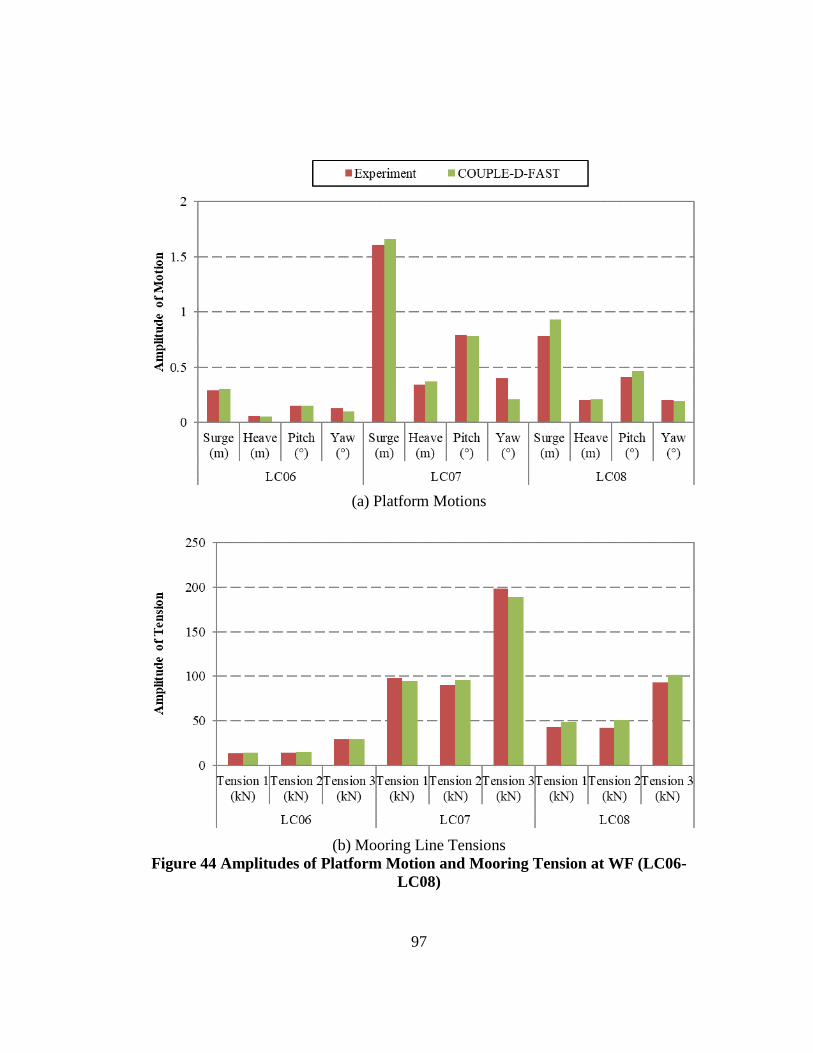
97
(a) Platform Motions
(b) Mooring Line Tensions
Figure 44 Amplitudes of Platform Motion and Mooring Tension at WF (LC06-
LC08)
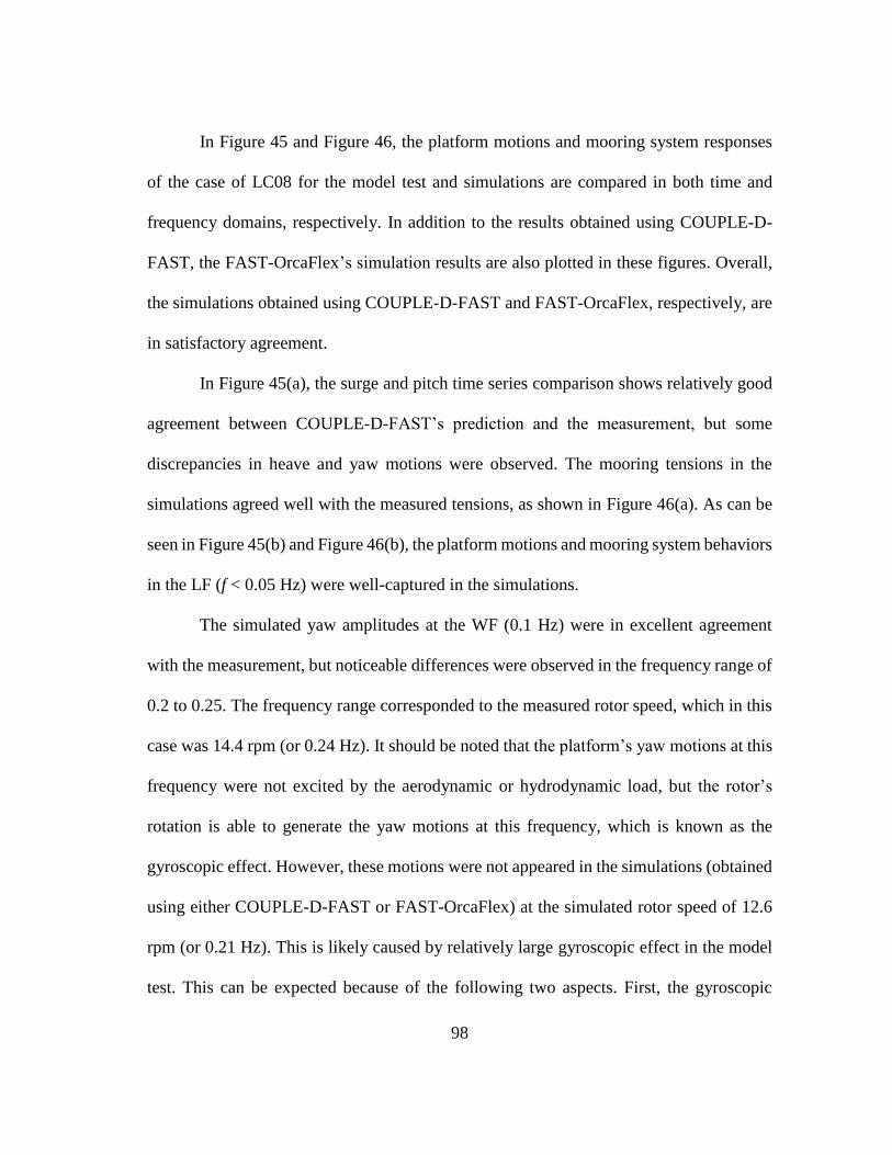
98
In Figure 45 and Figure 46, the platform motions and mooring system responses
of the case of LC08 for the model test and simulations are compared in both time and
frequency domains, respectively. In addition to the results obtained using COUPLE-D-
FAST, the FAST-OrcaFlex’s simulation results are also plotted in these figures. Overall,
the simulations obtained using COUPLE-D-FAST and FAST-OrcaFlex, respectively, are
in satisfactory agreement.
In Figure 45(a), the surge and pitch time series comparison shows relatively good
agreement between COUPLE-D-FAST’s prediction and the measurement, but some
discrepancies in heave and yaw motions were observed. The mooring tensions in the
simulations agreed well with the measured tensions, as shown in Figure 46(a). As can be
seen in Figure 45(b) and Figure 46(b), the platform motions and mooring system behaviors
in the LF (f < 0.05 Hz) were well-captured in the simulations.
The simulated yaw amplitudes at the WF (0.1 Hz) were in excellent agreement
with the measurement, but noticeable differences were observed in the frequency range of
0.2 to 0.25. The frequency range corresponded to the measured rotor speed, which in this
case was 14.4 rpm (or 0.24 Hz). It should be noted that the platform’s yaw motions at this
frequency were not excited by the aerodynamic or hydrodynamic load, but the rotor’s
rotation is able to generate the yaw motions at this frequency, which is known as the
gyroscopic effect. However, these motions were not appeared in the simulations (obtained
using either COUPLE-D-FAST or FAST-OrcaFlex) at the simulated rotor speed of 12.6
rpm (or 0.21 Hz). This is likely caused by relatively large gyroscopic effect in the model
test. This can be expected because of the following two aspects. First, the gyroscopic

99
frequency and the related moments induced by the rotor rotation were dominated by the
Reynolds number not by the Froude number. Secondly, likely uneven mass distributions
over the rotor’s plane with respect to its center may cause those large gyroscopic motions.
Figure 47 show a comparison of the yaw moments (or gyroscopic moments) at the tower
top in the COUPLE-D-FAST and FAST-OrcaFlex simulations, with the corresponding
measurements. As expected, the measured gyroscopic moments were much larger than the
simulated ones.

100
(a) Time series (b) Amplitude spectrum
Figure 45 Comparison of Platform Motions (LC08)

101
(a) Time series (b) Amplitude spectrum
Figure 46 Comparison of Mooring Tensions at Delta Joint (LC08)

102
Figure 47 Comparison of Tower-top Yaw Moments (LC08)
6.7. CASE IV: Impact of Turbulent Winds and Irregular Waves
Three cases (LC09 to LC11) of the Hywind FOWT’s dynamic behavior were
investigated under the impact of turbulent winds and irregular waves. The main
parameters of the three cases were listed in Table 12. The statistics of the FOWT’s
responses and mooring lines’ tensions for the Operational 1 (LC09), Operational 2 (LC10),
and Extreme (LC11) cases are summarized in Table 21. Most of the simulated results are
agree with the measurements. However, relatively large differences were observed in the
yaw motions. The discrepancies in average yaw may have been the result of the tested
wind conditions not being directly used in the simulations. The standard deviations in yaw
also rendered some discrepancies. It is mainly because the simulated yaw motions excited
by the rotor-rotations were not as large as the measurements.
Figure 48 and Figure 49 show the time series and amplitude spectra of the case of
LC11 for the platform motions and the mooring tensions at the joints for the measurements
and COUPLE-D-FAST and FAST-OrcaFlex predictions. In this case, irregular waves
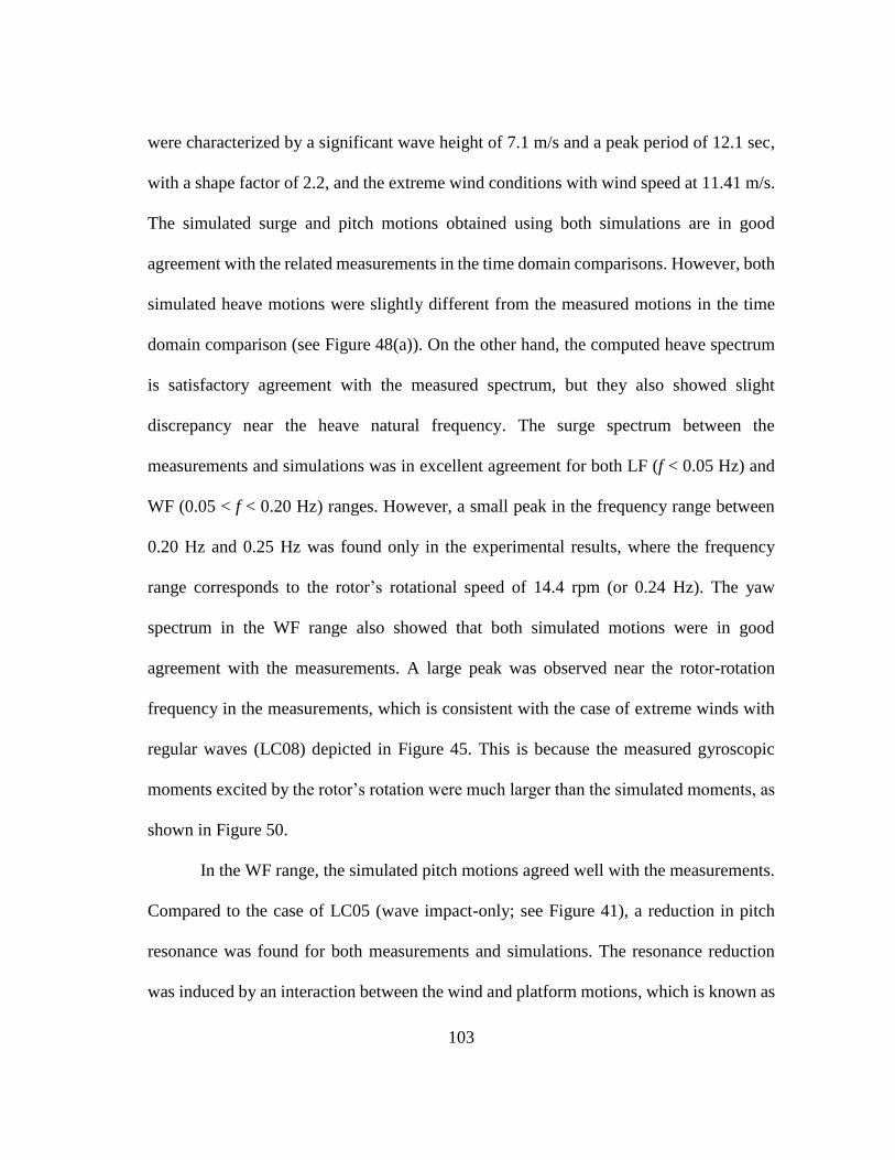
103
were characterized by a significant wave height of 7.1 m/s and a peak period of 12.1 sec,
with a shape factor of 2.2, and the extreme wind conditions with wind speed at 11.41 m/s.
The simulated surge and pitch motions obtained using both simulations are in good
agreement with the related measurements in the time domain comparisons. However, both
simulated heave motions were slightly different from the measured motions in the time
domain comparison (see Figure 48(a)). On the other hand, the computed heave spectrum
is satisfactory agreement with the measured spectrum, but they also showed slight
discrepancy near the heave natural frequency. The surge spectrum between the
measurements and simulations was in excellent agreement for both LF (f < 0.05 Hz) and
WF (0.05 < f < 0.20 Hz) ranges. However, a small peak in the frequency range between
0.20 Hz and 0.25 Hz was found only in the experimental results, where the frequency
range corresponds to the rotor’s rotational speed of 14.4 rpm (or 0.24 Hz). The yaw
spectrum in the WF range also showed that both simulated motions were in good
agreement with the measurements. A large peak was observed near the rotor-rotation
frequency in the measurements, which is consistent with the case of extreme winds with
regular waves (LC08) depicted in Figure 45. This is because the measured gyroscopic
moments excited by the rotor’s rotation were much larger than the simulated moments, as
shown in Figure 50.
In the WF range, the simulated pitch motions agreed well with the measurements.
Compared to the case of LC05 (wave impact-only; see Figure 41), a reduction in pitch
resonance was found for both measurements and simulations. The resonance reduction
was induced by an interaction between the wind and platform motions, which is known as

104
aerodynamic damping. One interesting phenomenon was that the degree of reduction in
pitch was different between the measurements and simulations. It is also observed that the
surge resonance motions between the measurements and simulations are in good
agreement. This indicates that the aerodynamic damping forces among the model test and
simulations were different. The damping difference may have been caused by the scale
effect from the Froude similitude because the aerodynamic damping follows the Reynolds
number scaling.
All computed tensions at the delta mooring joints were in satisfactory agreement
with the measurement in both time and frequency domain comparisons (see Figure 49).
However, some tension discrepancies were found in the LF range, which may be caused
by the differences in pitch resonance motions.

105
Table 21 Statistics for Platform Motions and Mooring Tensions (LC09-LC11) Mean SD Max Min
LC09
Surge (m) Experiment 3.316 0.221 4.068 2.659
Simulation 3.377 0.242 4.316 2.538
Heave (m) Experiment 0.153 0.051 0.349 -0.014
Simulation -0.037 0.034 0.084 -0.129
Pitch (°) Experiment 2.445 0.151 3.014 1.886
Simulation 2.211 0.149 2.698 1.764
Yaw (°) Experiment 0.344 0.753 1.928 -1.215
Simulation 0.036 0.081 0.325 -0.247
Tension 1
(kN)
Experiment 2870.3 16.5 2926.5 2810.5
Simulation 2853.1 12.4 2900.8 2807.1
Tension 2
(kN)
Experiment 2873.0 26.2 2961.2 2786.2
Simulation 2857.4 12.3 2905.1 2814.9
Tension 3
(kN)
Experiment 2599.0 31.0 2701.4 2492.3
Simulation 2581.4 24.0 2663.5 2481.1
LC10
Surge (m) Experiment 5.841 0.981 9.656 2.556
Simulation 5.557 1.103 9.443 1.526
Heave (m) Experiment -0.469 0.313 0.676 -1.581
Simulation -0.080 0.303 0.999 -1.094
Pitch (°) Experiment 4.520 0.484 6.267 2.818
Simulation 3.628 0.495 5.358 2.081
Yaw (°) Experiment 0.987 1.216 3.329 -1.551
Simulation 0.063 0.155 0.607 -0.536
Tension 1
(kN)
Experiment 2947.2 80.2 3224.8 2684.6
Simulation 2917.3 76.2 3228.2 2674.8
Tension 2
(kN)
Experiment 2941.7 99.9 3279.1 2599.7
Simulation 2923.3 78.3 3235.7 2673.0
Tension 3
(kN)
Experiment 2448.1 177.5 3027.2 1799.8
Simulation 2464.3 152.8 3072.6 1940.5
LC11
Surge (m) Experiment 8.679 1.039 13.540 5.252
Simulation 9.303 1.105 13.172 4.765
Heave (m) Experiment -0.595 0.318 0.481 -1.794
Simulation -0.268 0.299 0.890 -1.182
Pitch (°) Experiment 6.420 0.524 8.696 4.857
Simulation 6.075 0.509 7.668 4.218
Yaw (°) Experiment 1.256 1.135 3.733 -1.270
Simulation 0.133 0.178 0.771 -0.579
Tension 1
(kN)
Experiment 3037.1 81.2 3333.5 2747.1
Simulation 3026.8 74.8 3324.2 2787.5
Tension 2
(kN)
Experiment 3028.0 96.7 3415.0 2692.3
Simulation 3034.0 78.0 3335.4 2753.6
Tension 3
(kN)
Experiment 2306.3 179.5 2878.8 1681.2
Simulation 2264.7 154.7 2914.8 1732.1

106
(a) Time series (b) Amplitude spectrum
Figure 48 Comparison of Platform Motions (LC11)
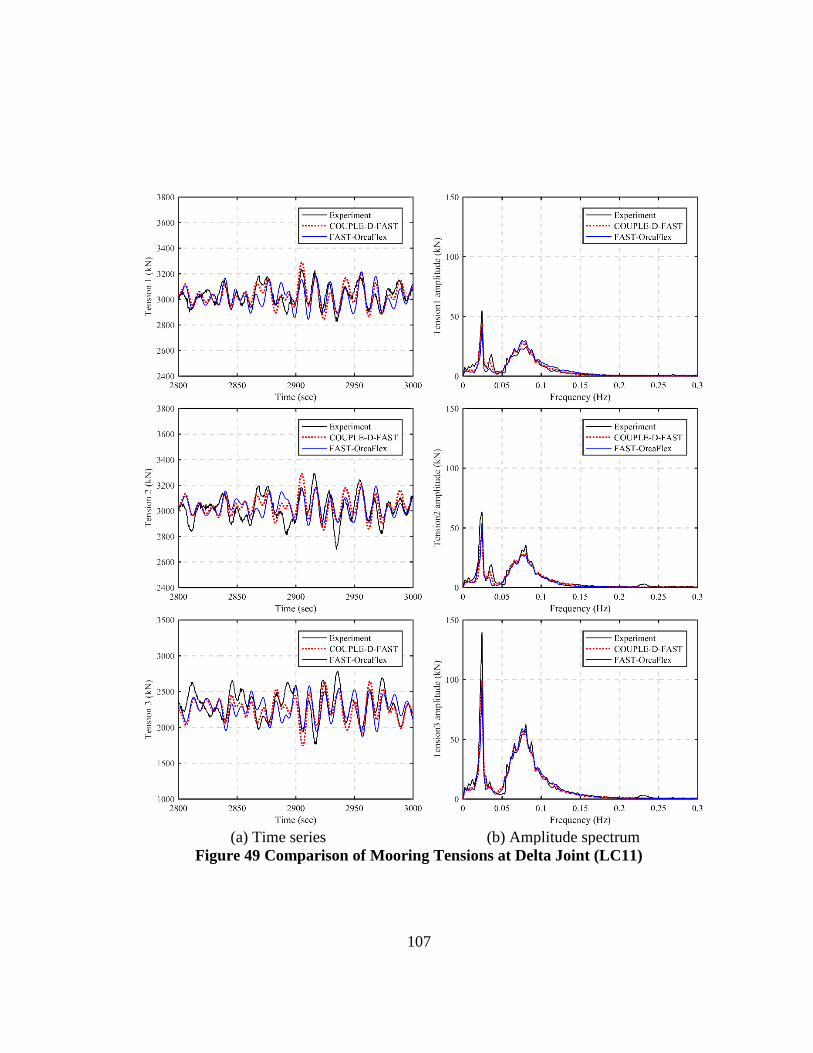
107
(a) Time series (b) Amplitude spectrum
Figure 49 Comparison of Mooring Tensions at Delta Joint (LC11)

108
Figure 50 Comparison of Tower-top Yaw Moments (LC11)

109
6.8. Discussion
In this section, COUPLE-D-FAST was verified through the comparisons of its
simulations with the related results of model tests. FAST-OrcaFlex was also used for the
simulation to examine the validity of COUPLE-D-FAST in certain cases where the
comparison between the measurements and simulations showed significant and/or
qualitative differences. The simulations using measured wind forces were implemented
using COUPLE-D only, mainly to investigate the sources causing the discrepancies in
mean motions (as described in Section 5.4) among the model test and simulations. The
simulations led to a correction of the center of gravity for the Hywind, which was changed
by approximately 3% closer to the water surface. The pitch free-decay test demonstrated
the validity of the CG correction, in that the case-specific increases in the moments of
inertia were no longer needed which were applied in our previous works (Min et al., 2016;
Min and Zhang, 2017). The CG correction led to the results that the simulated average
platform motions obtained in this research are in much better agreement with the measured
motions than that in our previous studies.
Eleven cases of various wind and wave conditions were simulated. The simulated
results were then compared to the corresponding measurements. The overall simulated
platform responses and mooring tensions agreed well with the measurements. In cases of
winds with irregular waves, the pitch resonances in the simulations were smaller than the
measured pitch resonances. This may have been caused by the different aerodynamic
damping which may result from the fact that the Froude similitude does not comply to the
scaling of aerodynamic forces. While the yaw resonances were barely visible in the

110
simulated results, the measurements showed large yaw resonances in the range of the
rotor-rotational frequency. This implies that the gyroscopic effects induced by the rotor’s
rotation in the model tests were larger than those in the simulation.

111
7. CONCLUSIONS
In this study, the CABLE3D module in COUPLE-FAST was extended to enable
the simulation of a delta mooring system. The extended COUPLE-FAST was named as
COUPLE-D-FAST. It was then used to investigate the dynamics of Hywind, a spar-type
FOWT with a delta mooring system. In most numerical simulations conducted in the
previous studies of Hywind, its delta mooring system was simplified to be a single
mooring system for the sake of simplicity, which needs empirical tuning and calibration
of its yaw stiffness and damping. The focus of this dissertation was to validate COUPLE-
D-FAST through comparisons with the related model tests and simulations using other
software, such as COUPLE-FAST and FAST-OrcaFlex.
The input to the numerical simulation carefully followed the major conditions and
settings of the model tests conducted in the wave basin. However, some features were
adjusted for the simplification of the computation. For example, the taper section of the
Hywind platform was approximated by a step cylinder. The following aspects of the
numerical model were carefully calibrated: mooring line stiffness, tower bending stiffness,
added-mass and drag coefficients of the platform.
The delta mooring system was modeled in the COUPLE-D-FAST and FAST-
OrcaFlex simulations without the simplification. For COUPLE-FAST, the empirically
calibrated yaw stiffness and damping were added, as has been done in the previous
research (Browning et al., 2012; Jonkman and Musial, 2010; Min et al., 2016). The
mooring surge and sway stiffness curves of all simulations and the related measurements
were in satisfactory agreement. The yaw stiffness curves calculated using COUPEL-D-
112
FAST and FAST-OrcaFlex, respectively, were in satisfactory agreement. The curves also
showed that the delta mooring system rendered a significantly large yaw stiffness
compared to the simplified mooring systems (without tuning the yaw stiffness) in
COUPLE-FAST.
COUPLE-D-FAST was initially calibrated by comparing its predictions with the
related free-decay tests. For translational motion, the simulated free-decay responses were
in good agreement with the corresponding measurements. In the yaw decay tests, the
effects of the yaw damping and stiffness related to the delta mooring system were captured
by COUPLE-D-FAST, and there was no need for additional case-specific tuning. In terms
of yaw damping effects, COUPLE-D-FAST was able to capture the damping effects better
than FAST-OrcaFlex.
Although Min and Zhang (2017) corrected the nominal wind speeds identified in
the model tests, the average motions of the Hywind FOWT was still smaller than those
recorded in the model tests. When the measured wind forces were directly input to the
simulations instead of those predicted by FAST, the predicted mean surge and pitch
motions rendered still smaller values compared to the mean motions in the model tests.
The smaller mean motions were likely caused by the hydrostatic pitch stiffness, which is
the dominant factor determining the mean pitch and surge of a spar-buoy platform at the
mean water level. To examine the effects of hydrostatic stiffness, we changed the
Hywind’s center of gravity by 3% closer to the calm water surface. The simulations using
the changed center of gravity showed that the average surge at the mean water level and
pitch motions were in satisfactory agreement with the related measurements. In addition,
113
there was no need to have an adjusted increase in the pitch moment of inertia to match the
pitch natural frequency, as did in our previous work (Min et al., 2016; Min and Zhang,
2017).
Eleven different cases were simulated and compared with the corresponding model
tests in order to validate COUPLE-D-FAST. These cases can be divided into four
different-load categories: wind load-only, irregular wave load-only, combined wind and
regular wave loads, and combined wind and irregular wave loads.
For the wind impact-only cases, the average platform motions predicted using
COUPLE-D-FAST showed satisfactory agreement with the corresponding measurements,
which is better than the results of our previous study (Min and Zhang, 2017). For the
irregular wave load-only cases, the phase of wave components obtained from for the
measured wave elevations was used for the simulation of the incident waves following the
corresponding JONSWAP spectrum. As expected, the simulated wave amplitude spectra
were similar to the related measured ones. The simulated FOWT’s global motion and
mooring tension at the delta joints showed satisfactory agreement with the corresponding
measurements in both time and frequency domains. In cases of regular waves combined
with wind, the mean position and dynamic response predicted using COUPLE-D-FAST
showed good agreement with the related model tests. Although some differences in the
surge amplitude at the wave frequency were observed, the magnitude of those differences
were very small (3 mm) in the model scale. For cases of irregular waves with wind, the
simulated FOWT’s behaviors, including motions and tensions, agreed very well with the
measurements in both time and frequency domain comparisons. The computed pitch
114
resonance in the LF range (near the natural frequencies of the surge and pitch) rendered a
relatively small response in comparison to those of the measurements. It is probably
caused by the different aerodynamic damping effects between the model tests and
simulations, because the aerodynamic damping effects follow the Reynolds number
instead of the Froude number.
The simulated yaw motion in the WF range showed satisfactory agreement with
the corresponding measurements. However, the simulated mean yaw motion showed
unsatisfactory agreement with the related measurements. Therefore, in addition to the
COUPLE-D-FAST simulations, FAST-OrcaFlex simulations were conducted to
investigate those discrepancies in the COUPLE-D-FAST simulations. It was shown that
the two numerical simulations were in good agreement in both time and frequency
domains. Yaw motions, other than the wave frequency, showed large discrepancies
between the simulations and the model tests. That is, the yaw motion induced by a
gyroscopic effect was barely observable in the simulations, while the model tests showed
relatively large yaw motions near the rotor-rotation frequency. The large yaw
discrepancies at the rotor-rotation frequency were expected. First, it is known that the
gyroscopic frequency and the related moments resulting from the blade rotation of the
wind turbine does not follow the Froude number scaling of the model tests to the
prototype. Secondly, likely uneven mass distribution over the rotor’s plane with respect to
its center in the model test may result in larger gyroscopic moments than those in the
simulations

115
Our research has shown that COUPLE-D-FAST can reliably and accurately
simulate the Hywind’s behaviors including its delta mooring system. The accurate
prediction of mooring tensions for all mooring segments of the delta mooring system will
contribute to FOWT design by providing key information such as fatigue life estimations
for mooring lines.

116
REFERENCES
Andersen, M. T., Wendt, F. F., Robertson, A. N., Jonkman, J. M., and Hall, M. 2016.
"Verification and Validation of Multisegmented Mooring Capabilities in Fast V8."
The 26th International Ocean and Polar Engineering Conference, Rhodes, Greece.
Aranha, J. 1994. "A Formula for ‘Wave Damping’in the Drift of a Floating Body."
Journal of Fluid Mechanics 275:147-155.
Bae, Y. H., Kim, M. H., Im, S. W., and Chang, I. H. 2011. "Aero-Elastic-Control-Floater-
Mooring Coupled Dynamic Analysis of Floating Offshore Wind Turbines." The
21st International Offshore and Polar Engineering Conference, Maui, Hawaii,
USA.
Browning, J., Jonkman, J., Robertson, A., and Goupee, A. 2012. "Calibration and
Validation of a Spar-Type Floating Offshore Wind Turbine Model Using the Fast
Dynamic Simulation Tool." Proceedings of the Science of Making Torque From
Wind, Oldenburg, Germany.
Cao, P., and Zhang, J. 1997. "Slow Motion Responses of Compliant Offshore Structures."
International Journal of Offshore and Polar Engineering 7 (02):119-126.
Chen, X. 2002. "Studies on Dynamic Interaction between Deep-Water Floating Structures
and Their Mooring/Tendon Systems." Doctor of Philosophy Thesis, Ocean
Engineering Program, Civil Engineering Department, Texas A&M University.
Clark, P., Malenica, Š., and Molin, B. 1993. "An Heuristic Approach to Wave Drift
Damping." Applied Ocean Research 15 (1):53-55.
117
Duan, F., Hu, Z., and Wang, J. 2015. "Model Tests of a Spar-Type Floating Wind Turbine
under Wind/Wave Loads." ASME 2015 34th International Conference on Ocean,
Offshore and Arctic Engineering, St. John's, Newfoundland, Canada.
Garrett, D. 1982. "Dynamic Analysis of Slender Rods." Journal of Energy Resources
Technology 104 (4):302-306.
Goupee, A. J., Koo, B. J., Kimball, R. W., Lambrakos, K. F., and Dagher, H. J. 2014.
"Experimental Comparison of Three Floating Wind Turbine Concepts." Journal
of Offshore Mechanics and Arctic Engineering 136 (2):020906-020906.
Hall, M., and Goupee, A. 2015. "Validation of a Lumped-Mass Mooring Line Model with
Deepcwind Semisubmersible Model Test Data." Ocean Engineering 104:590-
603.
Jonkman, B. J. 2009. Turbsim User's Guide: Version 1.50. National Renewable Energy
Laboratory, Golden, CO, USA.
Jonkman, J. M. 2007. Dynamics Modeling and Loads Analysis of an Offshore Floating
Wind Turbine. National Renewable Energy Laboratory, Golden, CO, USA.
Jonkman, J. M. 2010. Definition of the Floating System for Phase IV of OC3. National
Renewable Energy Laboratory, Golden, CO, USA.
Jonkman, J. M., Butterfield, S., Musial, W., and Scott, G. 2009. Definition of a 5-Mw
Reference Wind Turbine for Offshore System Development. National Renewable
Energy Laboratory, Golden, CO, USA.

118
Jonkman, J. M., and Musial, W. 2010. Offshore Code Comparison Collaboration (OC3)
for Iea Task 23 Offshore Wind Technology and Deployment. National Renewable
Energy Laboratory, Golden, CO, USA.
Kallesøe, B. S., and Hansen, A. M. 2011. "Dynamic Mooring Line Modeling in Hydro-
Aero-Elasticwind Turbine Simulations." The 21st International Offshore and Polar
Engineering Conference, Maui, Hawaii, USA.
Koo, B. J., Goupee, A. J., Kimball, R. W., and Lambrakos, K. F. 2012. "Model Tests for
a Floating Wind Turbine on Three Different Floaters." ASME 2012 31st
International Conference on Ocean, Offshore and Arctic Engineering, Rio de
Janeiro, Brazil.
Lindahl, J., and Sjoberg, A. 1983. "Dynamic Analysis of Mooring Cables." The Second
International Symposium on Ocean Engineering and Ship and Handling,
Gothenburg, Sweden.
Ma, W., and Webster, W. 1994. An Analytical Approach to Cable Dynamics: Theory and
User Manual. Sea Grant Project R/Oe-26. Department of Naval Architecture and
Offshore Engineering, University of California at Berkeley, CA, USA.
Martin, H. R., Kimball, R. W., Viselli, A. M., and Goupee, A. J. 2012. "Methodology for
Wind/Wave Basin Testing of Floating Offshore Wind Turbines." ASME 2012 31st
International Conference on Ocean, Offshore and Arctic Engineering, Rio de
Janeiro, Brazil.
Min, H., Peng, C., Duan, F., Hu, Z., and Zhang, J. 2016. "Numerical Simulation of
Dynamics of a Spar Type Floating Wind Turbine and Comparison with Laboratory
119
Measurements." ASME 2016 35rd International Conference on Ocean, Offshore
and Arctic Engineering, Busan, Korea.
Min, H., and Zhang, J. 2017. "Numerical Simulation of a Floating Offshore Wind Turbine
Constrained by Delta Mooring System." The 27th International Ocean and Polar
Engineering Conference, San Francisco, CA, USA.
Moriarty, P. J., and Hansen, A. C. 2005. Aerodyn Theory Manual. National Renewable
Energy Laboratory, Golden, CO, USA.
Musial, W., and Ram, B. 2010. Large-Scale Offshore Wind Power in the United States:
Assessment of Opportunities and Barriers. National Renewable Energy
Laboratory, Golden, CO, USA.
Nielsen, F. G., Hanson, T. D., and Skaare, B. r. 2006. "Integrated Dynamic Analysis of
Floating Offshore Wind Turbines." ASME 2006 25th International Conference on
Ocean, Offshore and Arctic Engineering, Hamburg, Germany.
Paulling, J., and Webster, W. C. 1986. "A Consistent, Large-Amplitude Analysis of the
Coupled Response of a Tlp and Tendon System." Proceedings Fifth International
Mechanics and Arctic Engineering Symposium, Tokyo, Japan.
Peng, C. 2015. "Numerical Study on a Spar Type Floating Offshore Wind Turbine Using
Couple-Fast Code." Doctor of Philosophy Thesis, Ocean Engineering Program,
Civil Engineering Department, Texas A&M University.
Peng, C., Yan, F., and Zhang, J. 2014. "Coupled Dynamic Response of a Spar Type
Floating Offshore Wind Turbine." ASME 2014 33rd International Conference on
Ocean, Offshore and Arctic Engineering, San Francisco, California, USA.
120
Quallen, S., Xing, T., Carrica, P., Li, Y., and Xu, J. 2013. "Cfd Simulation of a Floating
Offshore Wind Turbine System Using a Quasi-Static Crowfoot Mooring-Line
Model." The 23rd International Offshore and Polar Engineering Conference,
Anchorage, Alaska, USA.
Sarpkaya, T., and Isaacson, M. 1981. Mechanics of Wave Forces on Offshore Structures:
Van Nostrand Reinhold Company, NY, USA.
U.S.DOE. 2008. 20% Wind Energy by 2030: Increasing Wind Energy's Contribution to
U.S. Electricity Supply. Execute Summary. Springfield, VA, USA.
U.S.DOE. 2017a. 2016 Offshore Wind Technologies Market Report. Alexandria, VA,
USA.
U.S.DOE. 2017b. 2016 Wind Technologies Market Report. Alexandria, VA, USA.
Utsunomiya, T., Sato, I., Kobayashi, O., Shiraishi, T., and Harada, T. 2015. "Design and
Installation of a Hybrid-Spar Floating Wind Turbine Platform." ASME 2015 34th
International Conference on Ocean, Offshore and Arctic Engineering, St. John's,
Newfoundland, Canada.
Wendt, F. F., Andersen, M. T., Robertson, A. N., and Jonkman, J. M. 2016. "Verification
and Validation of the New Dynamic Mooring Modules Available in Fast V8." The
26th International Ocean and Polar Engineering Conference, Rhodes, Greece.
Zhang, J., Chen, L., Ye, M., and Randall, R. E. 1996. "Hybrid Wave Model for
Unidirectional Irregular Waves—Part I. Theory and Numerical Scheme." Applied
Ocean Research 18 (2–3):77-92.

121
APPENDIX A
SIMULATION RESULTS
1. LC01 (6.55 m/s Wind Only; Operational Condition 1)
1.1 Platform motions

122
1.2 Mooring tensions

123
2. LC02 (8.62 m/s Wind Only; Operational Condition 2)
2.1 Platform motions

124
2.2 Mooring tensions

125
3. LC03 (11.41 m/s Wind Only; Extreme Condition)
3.1 Platform motions

126
3.2 Mooring tensions
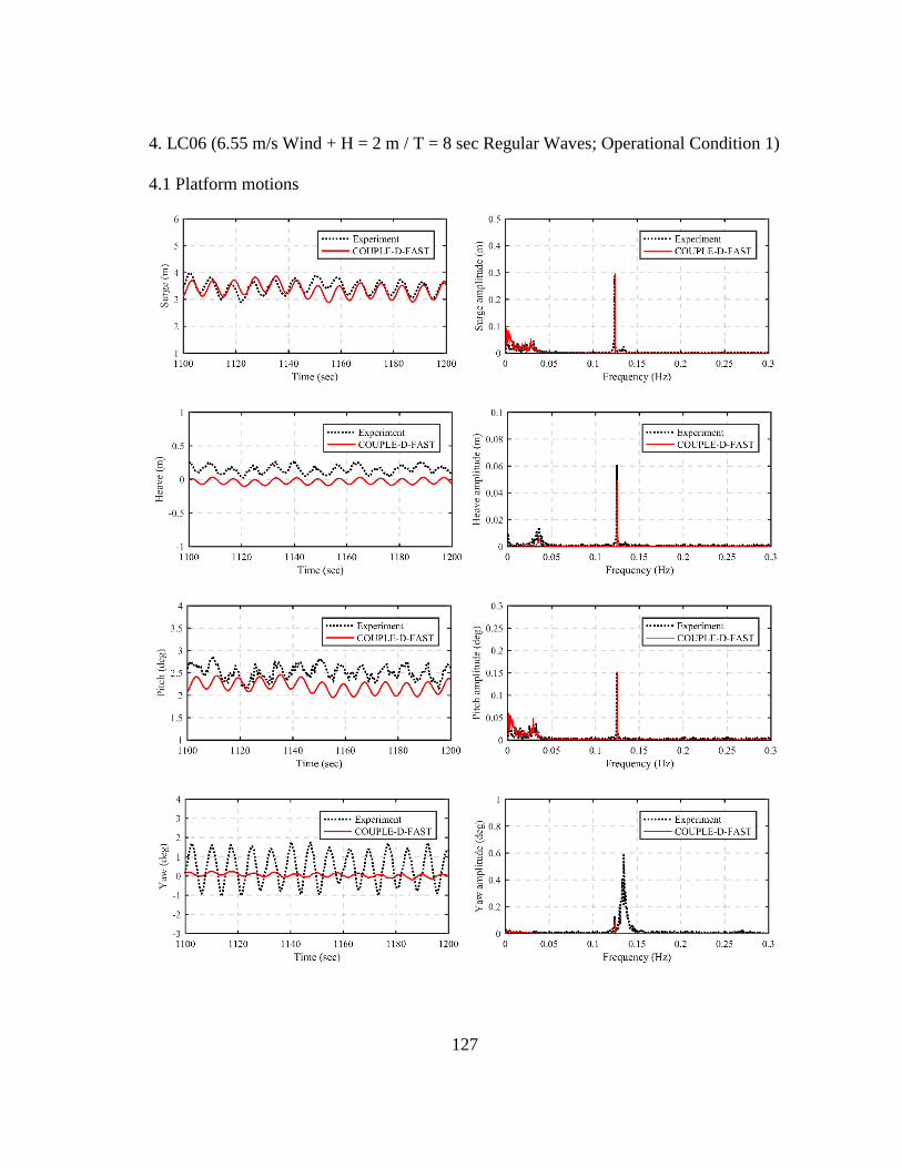
127
4. LC06 (6.55 m/s Wind + H = 2 m / T = 8 sec Regular Waves; Operational Condition 1)
4.1 Platform motions

128
4.2 Mooring tensions

129
5. LC07 (8.62 m/s Wind + H = 6 m / T = 11 sec Regular Waves; Operational Condition 2)
5.1 Platform motions
3

130
5.2 Mooring tensions

131
6. LC09
(6.55 m/s Wind + Hs = 2 m / Tp = 8 sec Irregular Waves; Operational Condition 1)
6.1 Platform motions

132
6.2 Mooring tensions
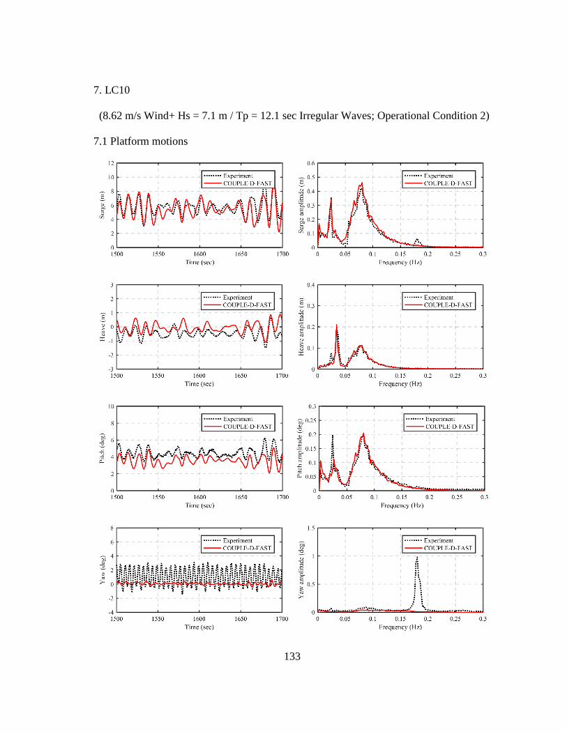
133
7. LC10
(8.62 m/s Wind+ Hs = 7.1 m / Tp = 12.1 sec Irregular Waves; Operational Condition 2)
7.1 Platform motions
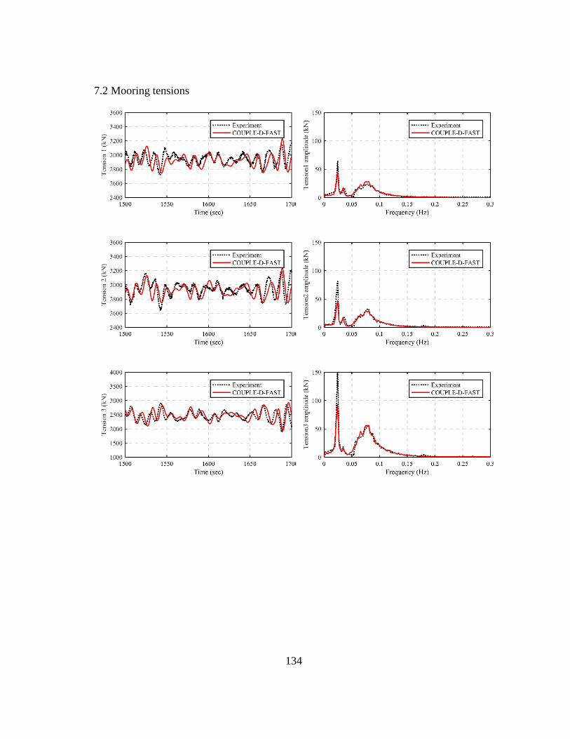
134
7.2 Mooring tensions