NUMERICAL SIMULATION OF ALUMINUM EXTRUSION PROCESSUSING SOLUTION ADAPTIVE FINITE ELEMENT METHOD

Mahender P. Reddy, Manas K. DebThe Computational Mechanics Company, Inc

:\ lIstin: TX 78752

and

J. Tinsley OdenTexas Institute for Computational and Applied Mathematics,

The University of Texas at AustinAustin. TX 78712

Sumbitted to Finite Elements in Analysis and DesignJanuary 1995

1

4-15

NUMERICAL SIMULATION OF ALUMINUM EXTRUSION PROCESSUSING SOLUTION ADAPTIVE FINITE ELEMENT METHOD

Mahender P. Reddy, Manas K. DebThe Computational Mechanics Company, Inc.,

Austin, TX 78752

and

J. Tinsley OdenTexas Institute for Computational and Applied Mathematics,

The University of Texas at AustinAustin, TX 78712

SUMMARY

Extrusion of two dimensional planar and axisymmetric aluminum sections is analyzedusing solution adaptive h-finite element method. The equations governing the flow of incom-pressible, non-Newtonian fluids are solved using an iterative penalty finite element model.An error estimation scheme based on the element residual method is used to obtain errorindicators. These indicators provide a basis for mesh refinement. The results from solutionadapted mesh are compared with those obtained after a series of uniform refinements of thecoarse mesh. Computed values for normal force on the die face with a solution adaptedmesh (399 elements for the planar extrusion and 477 for the axisymmetric case) were foundto be comparable (less than 0.4% for the planar section and 3% for the axisymmetric case)to those predicted with a fine mesh (1728 elements). These results indicate that reliablea-posteriori estimates of local errors in the numerical solution can be used provide a nearoptimal finite element mesh to solve complex problems.

1

INTRODUCTIONBackground

Extrusion is a commercially important process for the mass production of metal goods.Demands for high-speed production rates, increased product safety standards, and lowerenergy consumption have resulted in the increased use of numerical methods to predict theflow of metal during extrusion and other forming processes. A complete understanding ofthe flow field, temperature and load distribution, and behavior of the metal under variousoperating conditions is essential in selecting and optimizing the process variables such asthe extrusion rate, initial billet temperature, die design, and selection of proper equipment.

In the past, analytical methods such as the slip-line field methods [1]were used to analyzethe forming processes. These techniques allow the analysis of forces and flow in steady-stateprocesses for simple geometries. Nevertheless, forming processes are often unsteady and thegeometries are often complex. In addition, the extrusion process is highly nonlinear andthe simulation results are often sensitive to small changes in die geometry, temperature, diepressure, friction, and material characterization. Hence, classical analytical methods areseldom suitable for accurately determining the effect of various parameters on the metalflow.

It is now accepted that these shortcomings can be overcome by using modern numericalmethods such as the finite element method. Numerical methods, in principle, should enableone to conduct a systematic study of the effect of various parameters on the forming processeswhile providing understanding of the functionality of the process and the product thanpossible with experimental methods. When using numerical methods, one needs to ask thefollowing questions:

• how can one realistically model complex flow domains that are encountered commonlyin engineering practice?

• how accurate are the numerical solutions?, and

• is the grid fine enough to capture and resolve the flow behavior accurately?

The answer to the first question depends on the choice of mesh generation scheme. Itshould be emphasized that the numerical method being used to analyze the problem mustbe grid and coordinate system independent and also be able to automatically add or deletecells or grid points as needed to resolve the local solution errors. This can be achieved byusing unstructured grids, which is not feasible with mesh generators that use a body-fittedcoordinate system. The solution adaptive finite element methods satisfies these criteria andare well suited for modeling complex flow domains, and also enable the consistent impositionof gradient boundary conditions. In addition, the finite element method enables the userto obtain detailed solutions of the mechanics in the deforming body, such as: velocities,stresses, shear rates, temperature and pressure distributions.

The accuracy of the numerical solution depends on many factors: physical and math-ematical model of the flow phenomenon, the quality of numerical approximation, etc .. Inmetal extrusion, as in other forming processes, the material may undergo plastic deforma-tion. The plastic strains often outweigh elastic strains and the idealization of rigid-plastic

2

or rigid-viscoplastic material behavior is acceptable [2]. This assumption leads to what isknown as flow formulation. In flow formulation, one obtains the flow field by solving theequations governing the flow of incompressible non-Newtonian fluids in a given domain withappropriate constitutive relationship and boundary conditions. The finite element methodhas been used successfully to analyze extrusion and various forming process (See Ref. (2-6]and other similar works reported in literature).

Tradidonally, the accuracy of the numerical method can be established by comparingthe solution with available experimental data, which is usually very difficult to obtain forcomplex flow fields. In such instances, one creates a finite element mesh based on experienceand engineering judgment, and solves the problem. Then a second analysis is perfo.rmed bydoubling the mesh density. If there is a significant difference in the two solutions additionalrefinements are required until a mesh-independent solution is obtained. Such numericalexperiments are not always feasible when solving the complex problems encountered incommon engineering practice because of the time involved in regenerating the finite elementmesh and the computational cost in solving large problems.

In recent times, a new technology has emerged which promises to provide an alternativeto this traditional approach and which can be used for nonlinear processes. This technologycenters around the use of a reliable a-posteriori estimates of local errors in the numericalsolution; these provide a basis for mesh modification that can be directed to the regions ofthe domain where the solution is error is large. Using reliable information and hp-adaptationtechniques, the mesh in these critical regions can be redefined by either refining the elementsor enriching the interpolation basis for the elements.

This hp-adaptation and error-estimate strategy can remove the guess work from themesh generation process and can provide the user with a highly sophisticated tool to analyzecomplex flow problems starting with a very coarse mesh. Adaptive hp- finite element modelshave been used for the analysis of significant classes of incompressible flow problems [7-9].These techniques automatically adjust the element size h and its interpolation order p so asto deliver very high rates of convergence.

Present Study

In the present work, we apply the mesh adaptive methodologies to analyze steady-stateextrusion of visco-plastic materials (aluminum in particular). To this end, we analyzedtwo-dimensional planar and axisymmetric problems. First we analyzed the problems usingsuccessive mesh refinements (up to three levels) starting from an initial coarse mesh. Next,starting with the same initial coarse mesh, for each converged solution we estimated thelocal error in the solution and adapted the mesh by refining the elements with large errorsto produce an optimal mesh. The results from these refinement studies are presented.

In the next Section we describe the governing equations and the boundary conditionsfor the aluminum extrusion process. In Section 3 we describe the finite element model andadaptation strategies. Numerical results are presented in Section 4.

In this paper, we limit ourself to two-dimensional and axisymmetric flow geometries,and extension to three-dimensional geometries is straightforward. Also, only h-adaptationis used in the numerical experiments presented.

3

GOVERNING EQUATIONSConservation Equations

In aluminum extrusion process, as in other forming processes, the material undergoesplastic deformation. The plastic strains often outweigh elastic strains: and the idealizationof rigid-plastic or rigid-viscoplastic material behavior is acceptable [2]. This assumptionleads to what is known as flow formulation. In the flow formulation, the stress can bewritten as a function of the strain rate and a nonlinear viscosity relates the stress and strainrate.

Consider the steady flow of a non-isothermal, viscous, incompressible material in a closedregion n c JRn (n = 2, or 3). The laws of conservation of mass, linear momentum, andenergy can be used to derive the governing equations in terms of the velocity field, pressure,and temperature. In a rectangular Cartesian coordinate system (Xl, X2), these are given by

\7. u = a in np(u· \7)u = \7. u(u,p) + f in n

pCp( u . \7)T = -\7. q + Q + <I> in n

(1)(2)(3)

where u denotes the velocity vector, T is the temperature of the fluid, p is the mass densityof the fluid, Cp is the specific heat of the fluid at constant pressure, q is the heat fluxvector, Q denotes the volumetric heat source, <I> represents internal heat generation ratedue to viscous dissipation, f is the body force vector, u denotes the total stress tensor. Inthis study, the contributions of body force terms and volumetric heat source terms are notsignificant when compared to others and are henceforth neglected.

For viscous incompressible fluids, the components of the total stress tensor I u, can berepresented as the sum of the viscous (or deviatoric) part, T, and the hydrostatic part, -pI:

u = T - pI (4)

where p denotes the pressure and 1 is the unit tensor. The constitutive relations for theviscous stress tensor, T, and heat flux vector, q, respectively, are given by:

T

q

2µD(u)-k\7T

(5)(6)

where D (u) = (\7 u + \7u t) /2 are the components of the rate of the strain tensor, µ is theviscosity of the f:l.uid, which is a function of the temperature and rate of strain. k is theisotropic thermal conductivity of the material.

2.2 Constititive Relationship

For visco-plastic materials, the constitutive equations are expressed by [9]

?_uT=3iD(u)

4

(7)

where (; is the flow stress, which, in general, is a function of strain rate for a given temper-ature, and

(8)

is the effective strain rate. From Equations (5) and (7) we obtain,

(1

µ = 3€

The flow stress for aluminum depends on an internal state variable representing the materialmicrostructure (10]. An accurate description of the flow stress requires solving an evolu-tion equation which governs the internal variable. However, without the loss of valuableinformation, the flow stress can be approximated by the following empirical relations:

{ Z) lIn}(1 = ~ sinh - 1 (AZ = € exp (~)

(10)

(11)

where Z is the temperature dependent strain rate, Q is the activation energy, R is theuniversal gas constant, A is the reciprocal strain factor, a is a constant, and n is stressexponent.

Boun~ary Conditions

To complete the set of equations, Equations (1) - (3) need to be combined with anappropriate set of boundary conditions. Let r be the boundary of the domain n. For themomentum equation, the velocities (essential boundary condition) or the surface tractions(natural boundary condition) must be specified along the boundary. Similarly, for theenergy equations, the temperature (essential boundary condition) or the heat flux (naturalboundary condition)must be specified along the boundary. Let ru denote the boundary onwhich the velocities are specified, and rt be the boundary on which the stresses are specified.We have r = r u EB r t. Similarly, for the energy equation, r T denotes the boundary on whichthe temperature is specified, and rq represents the boundary on which the fluxes are specified(r = rT EB rq). Mathematically, the boundary conditions are:

on fuon rT

or

or (12)

where n denotes the outward unit normal vector on the boundary r. Note that pressureenters the natural boundary conditions through the total stress components.

5

FINITE ELEMENT MODELBackground

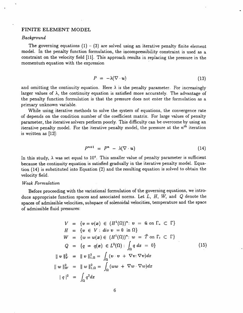
The governing equations (1) - (3) are solved using an iterative penalty finite elementmodel. In the penalty function formulation, the incompressibility constraint is used as aconstraint on the velocity field [11]. This approach results in replacing the pressure in themomentum equation with the expression .

p = ->'(\7. u) (13)

and omitting the continuity equation. Here"\ is the penalty parameter. For increasinglylarger values of >., the continuity equation is satisfied more accurately. The advantage ofthe penalty function formulation is that the pressure does not enter the formulation as aprimary unknown variable.

While using iterative methods to solve the system of equations, the convergence rateof depends on the condition number of the coefficient matrix. For large values of penaltyparameter, the iterative solvers perform poorly. This difficulty can be overcome by using aniterative penalty model. For the iterative penalty model, the pressure at the nth iterationis written as [12]:

pn+l = pn _ >'(\7. u) (14)

In this study, >. was set equal to 104. This smaller value of penalty parameter is sufficientbecause the continuity equation is satisfied gradually in the iterative penalty model. Equa-tion (14) is substituted into Equation (2) and the resulting equation is solved to obtain thevelocity field.

Weak Formulation

Before proceeding with the variational formulation of the governing equations, we intro-duce appropriate function spaces and associated norms. Let L, H, VV, and Q denote thespaces of admissible velocities, subspace of solenoidal velocities, temperature and the spaceof admissible fluid pressures:

v -H =W -

Q -

II v II~ -

II w II~v -

I q 12 =

{v = v(:z:) E (H1(n)t: v = u on f" C f}{v E v: div v = 0 in n}{w = w(:z:) E (H1(n)t: w = Ton ft C f}

{q = q(:z:) E L2(n) : in q dx = O}

IIv lIin = r (v· v + 'Vv:'Vv)dx, inIIw lIin = r (ww + \7w· \7w)dx. inin q2dx

6

(15)

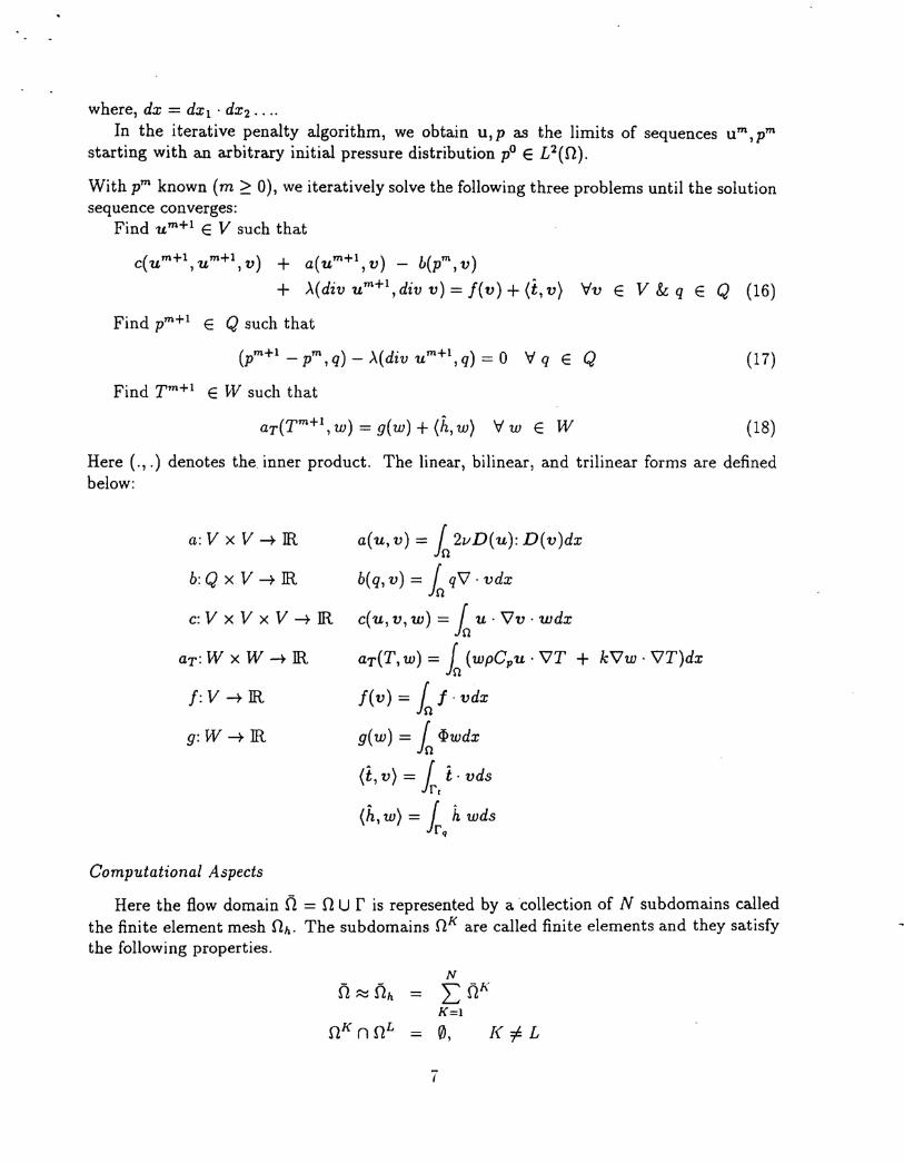
where, dx = dXl . dx2 ....In the iterative penalty algorithm, we obtain u, p as the limits of sequences um, pm

starting with an arbitrary initial pressure distribution pO E £2(0).

With pm known (m ~ 0), we iteratively solve the following three problems until the solutionsequence converges:

Find um+1 E V such that

c(um+l, um+l, v) + a(um+1, v) - b(pm, v)+ >"(div um+1,div v) = f(v) + (t,v) Vv E V & q E Q (16)

Find pm+l E Q such that

(pm+l _ pm,q) _ >"(div um+1,q) = 0 V q E Q

Find Tm+1 E W such that

aT(Tm+1,w)=g(w)+(h,w) Vw E W

(17)

(18)

Here (., .) denotes the inner product. The linear, bilinear, and trilinear forms are definedbelow:

a: V x V -+ IR a(u,v) = in 2vD(u): D(v)dx

b: Q x V -+ IR b(q,v) = in q\l. vdx

c: V x V x V -+ IR c(u, v, w) = in u· \lv . wdx

aT: W x W -+ IR aT(T, w) = k (wpCpu . VT + kVw· VT)dx

f: V -+ IR f (v) = in f .vdx

g: W -+ IR g(w) = in ipwdx

(t, v) = { t· vdsJrr

(h,w) = { h wdsJrq

Computational Aspects

Here the flow domain n = nUris represented by a collection of N subdomains calledthe finite element mesh nh. The subdomains OK are called finite elements and they satisfythe following properties.

NL nh'K=l

0, [( # L

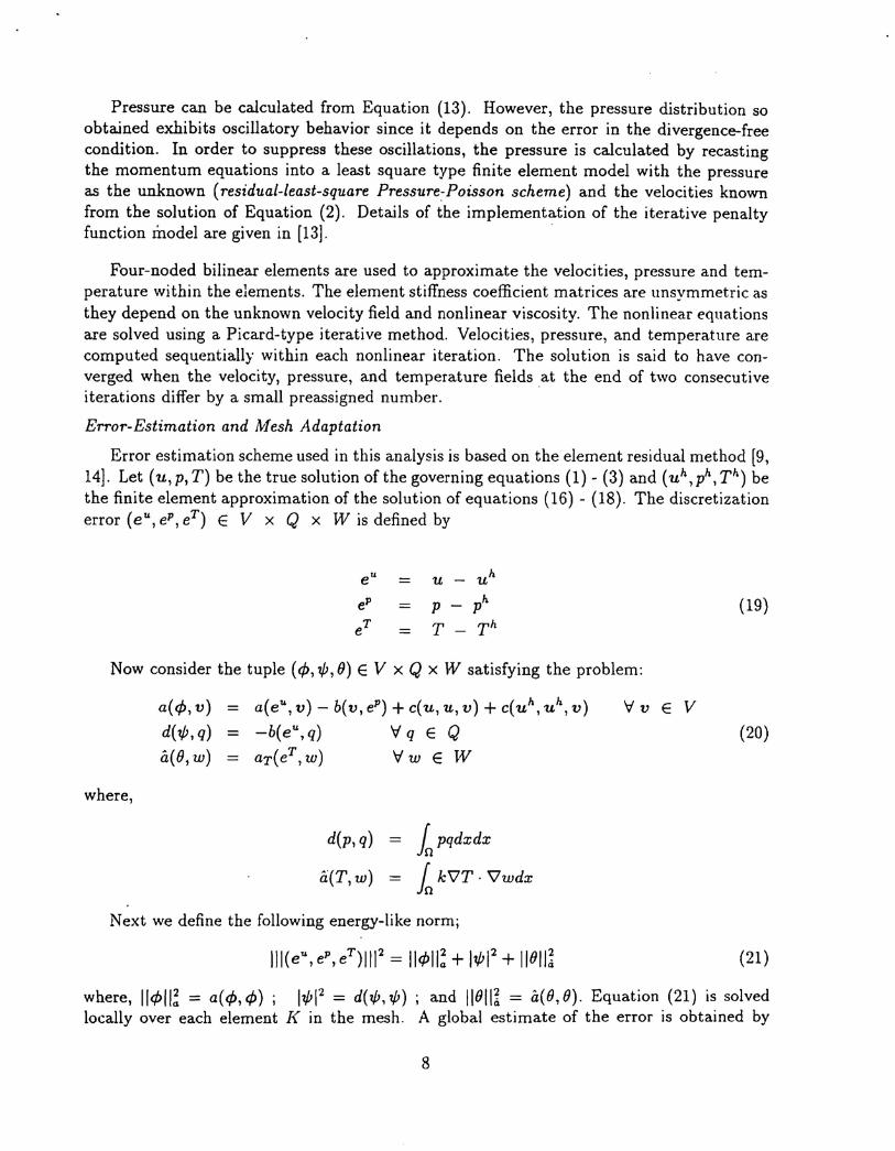
Pressure can be calculated from Equation (13). However, the pressure distribution soobtained exhibits oscillatory behavior since it depends on the error in the divergence-freecondition. In order to suppress these oscillations, the pressure is calculated by recastingthe momentum equations into a least square type finite element model with the pressureas the unknown (residual-least-square Pressure~Poisson scheme) and the velocities knownfrom the solution of Equation (2). Details of the implementation of the iterative penaltyfunction model are given in [13].

Four-noded bilinear elements are used to approximate the velocities, pressure and tem-perature within the elements. The element stiffness coefficient matrices are unsymmetric asthey depend on the unknown velocity field and nonlinear viscosity. The nonlinear equationsare solved using a Picard-type iterative method. Velocities, pressure, and temperature arecomputed sequentially within each nonlinear iteration. The solution is said to have con-verged when the velocity, pressure, and temperature fields at the end of two consecutiveiterations differ by a small preassigned number.

Error-Estimation and Mesh Adaptation

Error estimation scheme used in this analysis is based on the element residual method [9,14]. Let (u, p, T) be the true solution of the governing equations (1) - (3) and (uh, ph, Th) bethe finite element approximation of the solution of equations (16) - (18). The discretizationerror (eU

, eP, eT) E V x Q x W is defined by

eU = u - uh

eP - p _ ph (19)eT - T - Th

Now consider the tuple (4),''µ, 0) E V x Q x HI satisfying the problem:

where,

a(4), v)d("µ,q)a(O, w)

a(eU, v) - b(v, eP) + c(u, u, v) + c(uh, uh, v)

-b(eU,q) V q E QaT(eT,w) Vw E W

Vv E V(20)

d(p, q)

Ci(T, w)

kpqdxdx

in k\lT . '\lwdx

Next we define the following energy-like norm;

(21)

where, 114>1I~ = a(4),4>); 1.,µ12 = d("µ,"µ) ; and 110m = a(O,fJ). Equation (21) is solvedlocally over each element [{ in the mesh. A global estimate of the error is obtained by

8

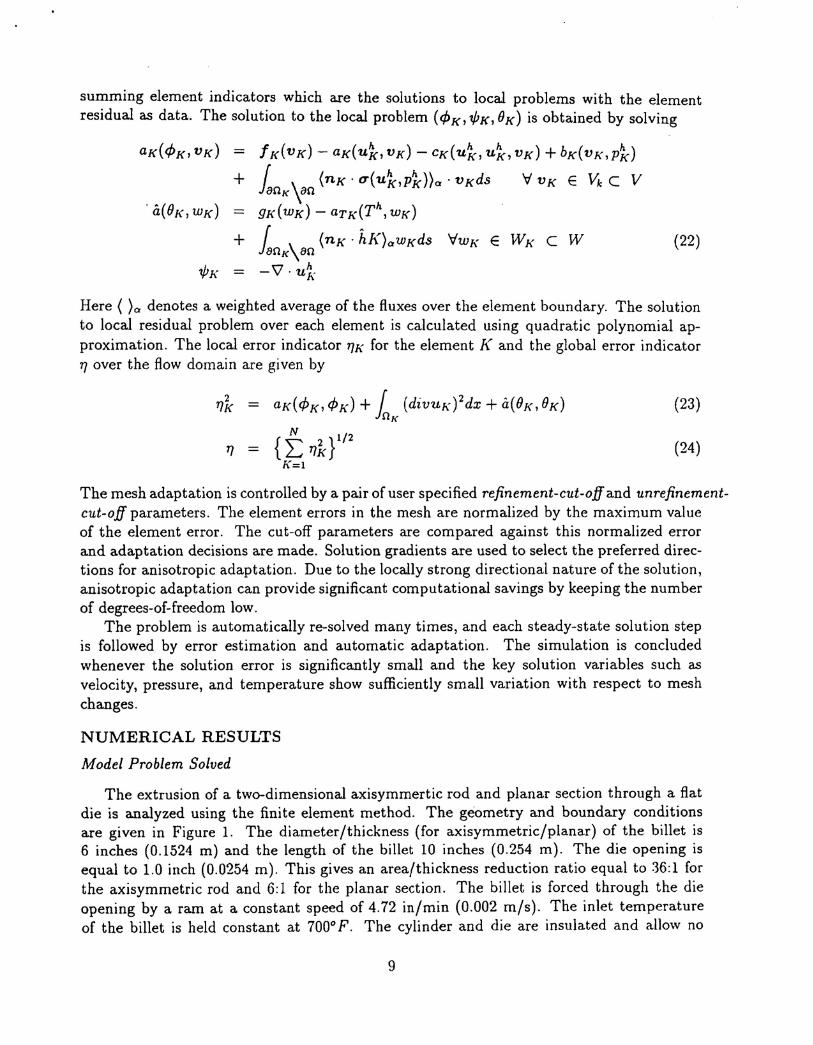
summing element indicators which are the solutions to local problems with the elementresidual as data. The solution to the local problem (tPK, .,pK, OK) is obtained by solving

- fK(VK) - aK(uk, VK) - cK(uk, uk, VK) + bK(VK,pk)

+ [ \ (nK' u(uk,Pk))a . vKds 'V VK E Vk C VlanK an- gK(WK) - aTK(Th,wK)

+ [ \ (nK . hK)awKds 'VWK E WK C WlanK an= -V'. u~

(22)

Here ( )a denotes a weighted average of the fluxes over the element boundary. The solutionto local residual problem over each element is calculated using quadratic polynomial ap-proximation. The local error indicator 17K for the element K and the global error indicator17over the flow domain are given by

(23)

(24)

The mesh adaptation is controlled by a pair of user specified refinement-cut-off and unrefinement-cut-off parameters. The element errors in the mesh are normalized by the maximum valueof the element error. The cut-off parameters are compared against this normalized errorand adaptation decisions are made. Solution gradients are used to select the preferred direc-tions for anisotropic adaptation. Due to the locally strong directional nature of the solution,anisotropic adaptation can provide significant computational savings by keeping the numberof degrees-of-freedom low.

The problem is automatically re-solved many times, and each steady-state solution stepis followed by error estimation and automatic adaptation. The simulation is concludedwhenever the solution error is significantly small and the key solution variables such asvelocity, pressure, and temperature show sufficiently small variation with respect to meshchanges.

NUMERICAL RESULTS

Model Problem Solved

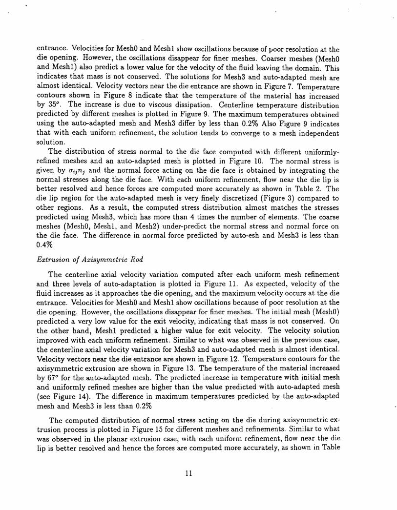
The extrusion of a two-dimensional axisymmertic rod and planar section through a flatdie is analyzed using the finite element method. The geometry and boundary conditionsare given in Figure 1. The diameter/thickness (for axisymmetric/planar) of the billet is6 inches (0.1524 m) and the length of the billet 10 inches (0.254 m). The die opening isequal to 1.0 inch (0.0254 m). This gives an area/thickness reduction ratio equal to 36:1 forthe axisymmetric rod and 6:1 for the planar section. The billet is forced through the dieopening by a ram at a constant speed of 4.72 in/min (0.002 m/s). The inlet temperatureof the billet is held constant at 7000 F. The cylinder and die are insulated and allow no

9

slip. The material properties of aluminum and the constants in Equations (10) and (11) aregiven in Table 1

As mentioned in the Introduction, the aim of this study is to apply mesh adaptivemethodologies to analyze the steady-state extrusion of visco-plastic materials (aluminum inparticular). To illustrate the advantages of using adaptation techniques with an a posteriorierror estimate, we first solve the problem (for both axisymmetric and planar cases) using aseries of uniformly refined meshes. Next, y;e solve the same problem using the adaptationtechniques explained above. The relative accuracy of the numerical solution is determinedby comparing two sets of results (die force, centerline velocity, and temperature).

Figure 2 shows the initial mesh, consisting of 27 bilinear elements and 40 nodes. Startingwith this coarse mesh, the mesh is uniformly refined three times to obtain three mesheswith 108, 432, and 1728 elements, respectively. The successive finer meshes are obtained bydividing each element in the previous coarse mesh into four smaller elements of same aspectratio. In other words, the 108 elements mesh is obtained by dividing each element in the 27element mesh into four smaller elements of equal area.

For mesh adaptation based on error estimation, we solve the same problem using theadaptation strategy explained in the previous section. For each converged solution startingwith the initial coarse mesh, the error indicators are computed and the mesh is automat-ically adapted in the regions where the normalized relative error is larger than the speci-fied value. Appropriate norms of solution gradients are used to select preferred directionsfor anisotropic adaptation. Due to the locally strong directional nature of the solution,anisotropic adaptation can provide significant computational savings by keeping the num-ber of degrees-of-freedom low. The mesh adaptation is stopped when the solution error andcbanges in the key solution variables such as the velocities, pressure, and temperature aresufficiently small.

The numerical results are presented below. As expected, the quality of the solution interms of the computed velocity, pressure, and temperature distribution is improved witheach refinement. For clarity and ease of explanation, we refer to the initial mesh as MeshO.Meshl, Mesh2, and Mesh3 are the meshes obtained after one-, two-, and three- uniformrefinements of MeshO. Figures 3 and 4 show the finite element mesh obtained after threelevels of auto-adaptation for the planar and axisymmetric cases. The auto-adapted meshfor the planar case consists of 399 elements and 492 nodes and that of the axisymmetriccase consists of 477 elements and 576 nodes. In these meshes, the element density is morenear regions where large variations in the solution take place (such as the die entrance andother singularities). The finite element mesh after three uniform refinements (Mesh3) isshown in Figure 5. Comparing meshes in Figures 3 and 4 with the one shown in Figure 5indicates that in Mesh3 large number of elements are placed in regions of little importance.It should be pointed 'out that for complex geometries, it would be difficult to manuallygenerate meshes similar to those shown in Figures 3 and 4.

Planar Extrusion

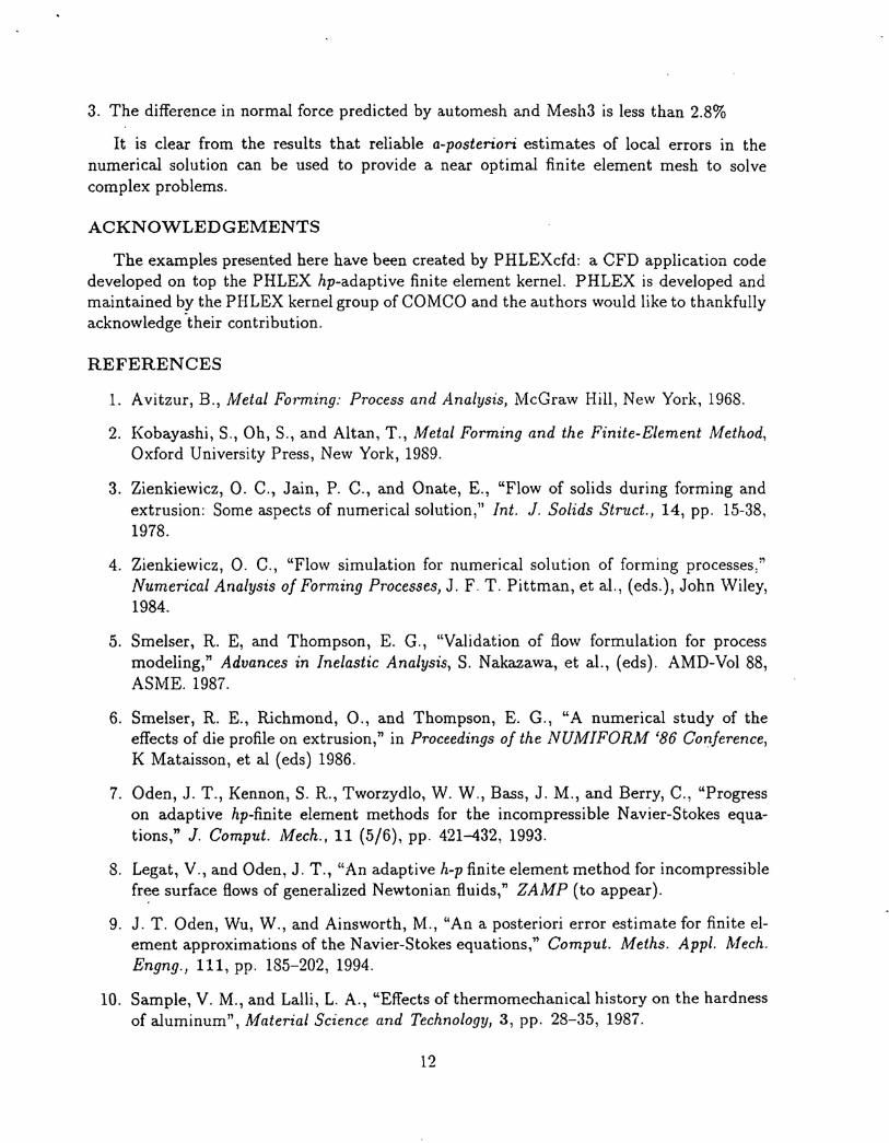
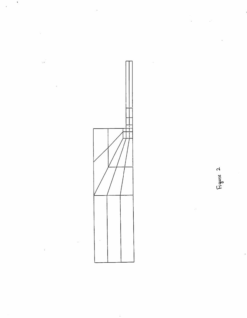
Centerline axial velocity variation computed after each uniform mesh refinement andthree levels of auto-adaptation is plotted in Figure 6. The axial velocity increases as thefluid particles reach the die opening. As expected the maximum velocity occurs at the die

10

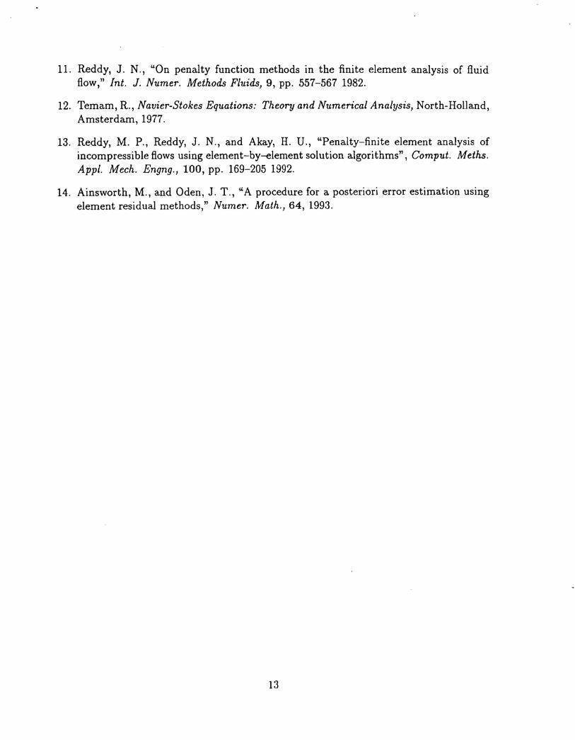
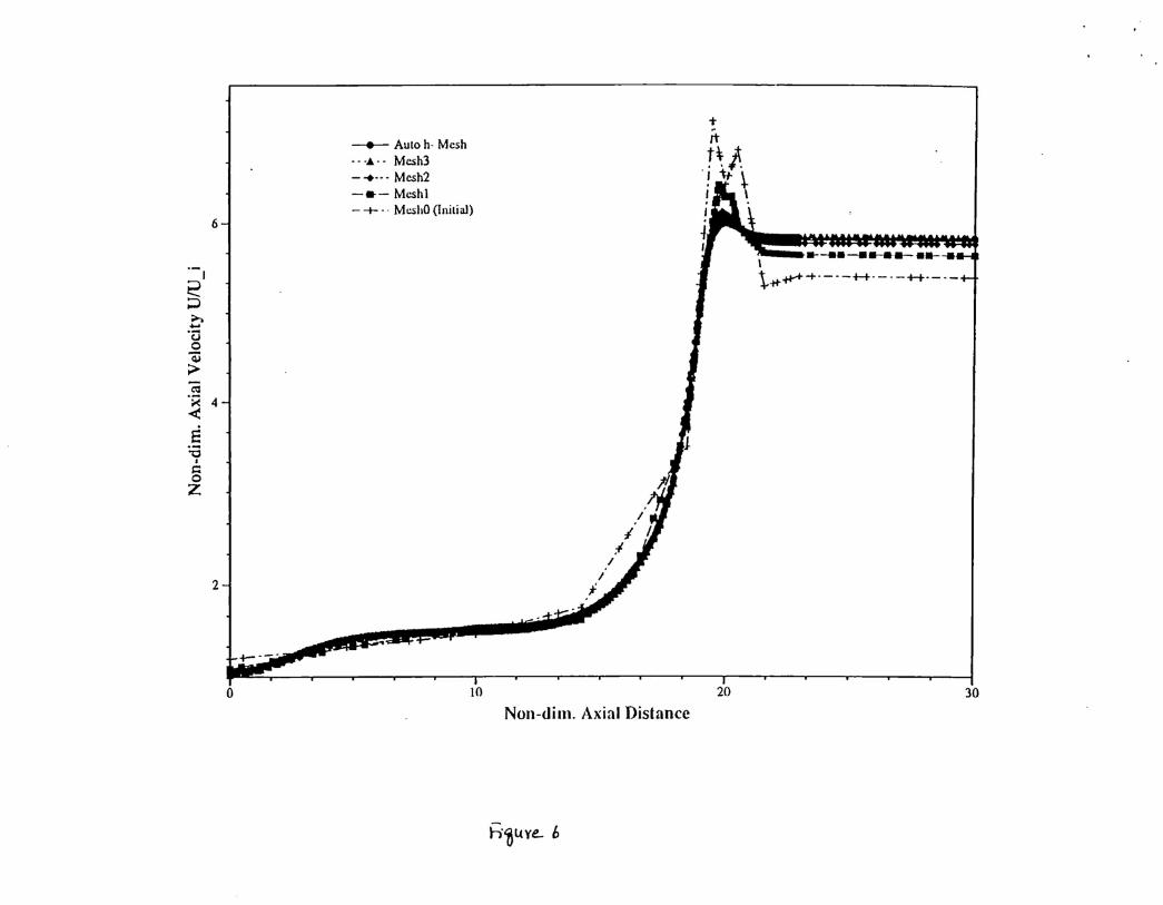
entrance. Velocities for MeshO and Meshl show oscillations because of poor resolution at thedie opening. However, the oscillations disappear for finer meshes. Coarser meshes (MeshOand Meshl) also predict a lower value for the velocity of the fluid leaving the domain. Thisindicates that mass is not conserved. The solutions for Mesh3 and auto-adapted mesh arealmost identical. Velocity vectors near the die entrance are shown in Figure 7. Temperaturecontours shown in Figure 8 indicate that the temperature of the material has increasedby 35°. The increase is due to viscous dissipation. Centerline temperature distributionpredicted by different meshes is plotted in Figure 9. The maximum temperatures obtainedusing the auto-adapted mesh and Mesh3 differ by less than 0.2% Also Figure 9 indicatesthat with each uniform refinement, the solution tends to converge to a mesh independentsolution.

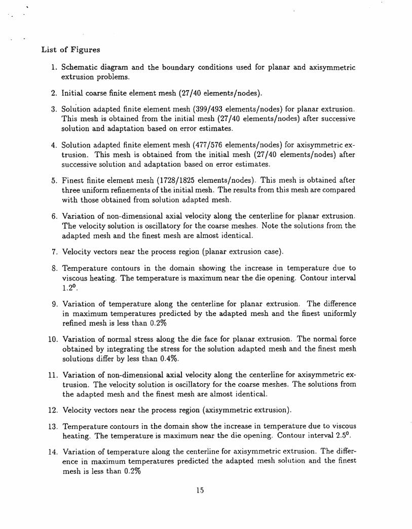
The distribution of stress normal to the die face computed with different uniformly-refined meshes and an auto-adapted mesh is plotted in Figure 10. The normal stress isgiven by G'ijnj and the normal force acting on the die face is obtained by integrating thenormal stresses along the die face. With each uniform refinement, flow near the die lip isbetter resolved and hence forces are computed more accurately as shown in Table 2. Thedie lip region for the auto-adapted mesh is very finely discretized (Figure 3) compared toother regions. As a result, the computed stress distribution almost matches the stressespredicted using Mesh3, which has more than 4 times the number of elements. The coarsemeshes (MeshO, Meshl, and Mesh2) under-predict the normal stress and normal force onthe die face. The difference in normal force predicted by auto-esh and Mesh3 is less than0.4%

Extrusion of Axisymmetric Rod

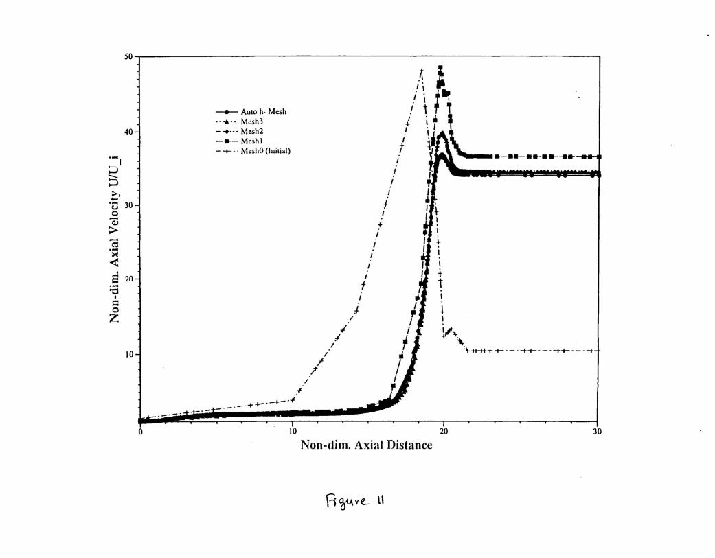
The centerline axial velocity variation computed after each uniform mesh refinementand three levels of auto-adaptation is plotted in Figure 11. As expected, velocity of thefluid increases as it approaches the die opening, and the maximum velocity occurs at the dieentrance. Velocities for MeshO and Meshl show oscillations because of poor resolution at thedie opening. However, the oscillations disappear for finer meshes. The initial mesh (MeshO)predicted a very low value for the exit velocity, indicating that mass is not conserved. Onthe other hand, Meshl predicted a higher value for exit velocity. The velocity solutionimproved with each uniform refinement. Similar to what was observed in the previous case,the centerline axial velocity variation for Mesh3 and auto-adapted mesh is almost identical.Velocity vectors near the die entrance are shown in Figure 12. Temperature contours for theaxisymmetric extrusion are shown in Figure 13. The temperature of the material increasedby 67° for the auto-adapted mesh. The predicted increase in temperature with initial meshand uniformly refined meshes are higher than the value predicted with auto-adapted mesh(see Figure 14). The difference in maximum temperatures predicted by the auto-adaptedmesh and Mesh3 is less than 0.2%

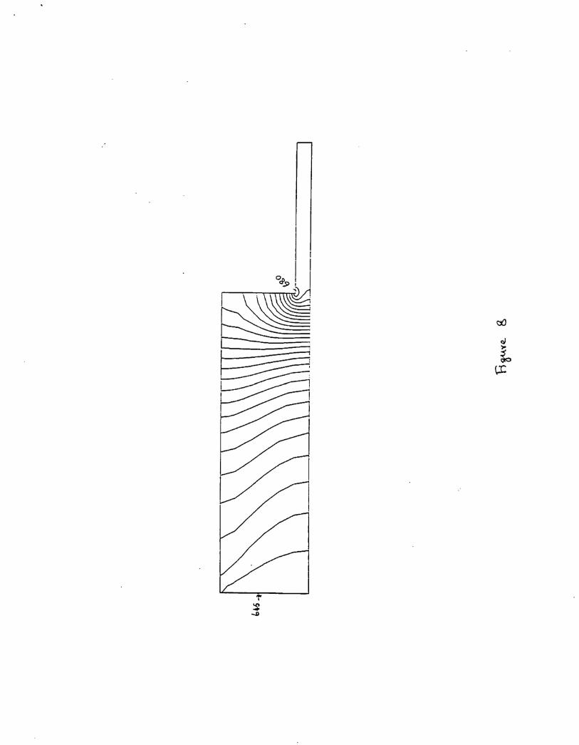
The computed distribution of normal stress acting on the die during axisymmetric ex-trusion process is plotted in Figure 15 for different meshes and refinements. Similar to whatwas observed ill the planar extrusion case, with each uniform refinement, flow near the dielip is better resolved and hence the forces are computed more accurately, as shown in Table

11

3. The difference in normal force predicted by automesh and Mesh3 is less than 2.8%

It is clear from the results that reliable a-posteriori estimates of local errors in thenumerical solution can be used to provide a near optimal finite element mesh to solvecomplex problems.

ACKNOWLEDGEMENTS

The examples presented here have been created by PHLEXcfd: a CFD application codedeveloped on top the PHLEX hp-adaptive finite element kernel. PHLEX is developed andmaintained by the PHLEX kernel group of COMCO and the authors would like to thankfullyacknowledge -their contribution.

REFERENCES

1. Avitzur, B., Metal Forming: Process and Analysis, McGraw Hill, New York, 1968.

2. Kobayashi, S., Oh, S., and Altan, T., Metal Forming and the Finite-Element Method,Oxford University Press, New York, 1989.

3. Zienkiewicz, O. C., Jain, P. C., and Onate, E., "Flow of solids during forming andextrusion: Some aspects of numerical solution," Int. J. Solids Struct., 14, pp. 15-38,1978.

4. Zienkiewicz, O. C., "Flow simulation for numerical solution of forming processes,"Numerical Analysis of Forming Processes, J. F. T. Pittman, et a1., (eds.), John \Viley,1984.

5. Smelser, R. E, and Thompson, E. G., "Validation of flow formulation for processmodeling," Advances in Inelastic Analysis, S. Nakazawa, et aI., (eds). AMD-VoI88,ASME.1987.

6. Smelser, R. E., Richmond, 0., and Thompson, E. G., "A numerical study of theeffects of die profile on extrusion," in Proceedings of the NUMIFORM '86 Conference,K Mataisson, et al (eds) 1986.

7. aden, J. T., Kennon, S. R., Tworzydlo, W. W., Bass, J. M., and Berry, C., "Progresson adaptive hp-finite element methods for the incompressible Navier-Stokes equa-tions," J. Comput. l\1ech., 11 (5/6), pp. 421-432, 1993.

8. Legat, V., and Oden, J. T., "An adaptive h-p finite element method for incompressiblefree surface flows of generalized Newtonian fluids," ZAMP (to appear).

9. J. T. Oden, Wu, W., and Ainsworth, M., "An a posteriori error estimate for finite el-ement approximations of the Navier-Stokes equations," Comput. Meths. Appl. Mech.Engng., 111, pp. 185-202, 1994.

10. Sample, V. M., and Lalli, L. A., "Effects of thermomechanical history on the hardnessof aluminum", Material Science and Technology, 3, pp. 28-35, 1987.

12

11. Reddy, J. N., "On penalty function methods in the finite element analysis of fluidflow," Int. J. Numer. Methods Fluids, 9, pp. 557-567 1982.

12. Temam, R., Navier-Stokes Equations: Theory and Numerical Analysis, North-Holland,Amsterdam, 1977.

13. Reddy, M. P., Reddy, J. N., and Akay, H. U., "Penalty-finite element analysis ofincompressible flows using element-by-element solution algorithms", Comput. Meths.Appl. Mech. Engng., 100, pp. 169-205 1992.

14. Ainsworth, M., and Oden, J. T., "A procedure for a posteriori error estimation usingelement residual methods," Numer. Math., 64, 1993.

13

Table 1: Material properties for aluminum.Cp = 1.076J/gm-I<k = 224 W/ m - I<p = 2664 I<g/m3

Q = 0.03224 MPa-1

A = 8.5761 1/ Sec.Q = 177200 J/gm - molR = 8.3213 J /mol - I< - gmn = 4.75

Table 2. Normal force on the die (planar extrusion).

Elements Nodes Force (!vI N) Remarks27 40 3.17439 MeshO (Ini tial Mesh)

108 133 3.81281 Meshl (1 Uniform Refinement)432 481 4.28364 Mesh2 (2 Uniform Refinements)

1728 1825 4.63250 Mesh3 (3 Uniform Refinements)399 492 4.64996 Auto-Mesh(3 Auto Adaptation Steps)

Table 3. Normal force on the die (axisymmetric extrusion).

Elements Nodes Force (MN) Remarks27 40 0.28056 MeshO (Initial Mesh)

108 133 1.72938 Mesh1 (1 Uniform Refinement)432 481 1.99436 Mesh2 (2 Uniform Refinements)

1728 1825 2.15672 Mesh3 (3 Uniform Refinements)477 576 2.09450 Auto-Mesh(3 Auto Adaptation Steps)

14

List of Figures

1. Schematic diagram and the boundary conditions used for planar and axisymmetricextrusion problems.

2. Initial coarse finite element mesh (27/40 elements/nodes).

3. Solution adapted finite element mesh (399/493 elements/nodes) for planar extrusion.This mesh is obtained from the initial mesh (27/40 elements/nodes) after successivesolution and adaptation based on error estimates.

4. Solution adapted finite element mesh (477/576 elements/nodes) for axisymmetric ex-trusion. This mesh is obtained from the initial mesh (27/40 elements/nodes) aftersuccessive solution and adaptation based on error estimates.

5. Finest finite element mesh (1728/1825 elements/nodes). This mesh is obtained afterthree uniform refinements of the initial mesh. The results from this mesh are comparedwith those obtained from solution adapted mesh.

6. Variation of non-dimensional axial velocity along the centerline for planar extrusion.The velocity solution is oscillatory for the coarse meshes. Note the solutions from theadapted mesh and the finest mesh are almost identical.

7. Velocity vectors near the process region (planar extrusion case).

8. Temperature contours in the domain showing the increase in temperature due toviscous heating. The temperature is maximum near the die opening. Contour interval1.2°.

9. Variation of temperature along the centerline for planar extrusion. The differencein maximum temperatures predicted by the adapted mesh and the finest uniformlyrefined mesh is less than 0.2%

10. Variation of normal stress along the die face for planar extrusion. The normal forceobtained by integrating the stress for the solution adapted mesh and the finest meshsolutions differ by less than 0.4%.

11. Variation of non-dimensional axial velocity along the centerline for axisymmetric ex-trusion. The velocity solution is oscillatory for the coarse meshes. The solutions fromthe adapted mesh and the finest mesh are almost identical.

12. Velocity vectors near the process region (axisymmetric extrusion).

13. Temperature contours in the domain show the increase in temperature due to viscousheating. The temperature is maximum near the die opening. Contour interval 2.5°.

14. Variation of temperature along the centerline for axisymmetric extrusion. The differ-ence in maximum temperatures predicted the adapted mesh solution and the finestmesh is less than 0.2%

15

15. Variation of normal stress along the die face for axisymmetric extrusion. The normalforce obtained by integrating the stress for the solution adapted mesh and the finestmesh solutions differ by less than 3.0%.

16

Cylinder U == 0, q.ll == 0

Product t 0.0254 m-.-.-".-.-.-.-.-.-.-.---.-.-.-.-.-.-.---.-.-.-.-.-.-.-.-.---.-.

Symmetry Plane V.1l == 0, 't == 0, q.1l == 0f

~ ~~ J0.254 m 0.127 In

Ram/pistonU == 0.002 m/secV==oT == 645 K

0.1524 m Billet

Die Face[J == 0, q.1I == 0

Free Sllfface V.Il::= 0, q.1l :()

Outflowp==o't == 't ::= 0I n

q.1l == 0

Fi~UYe- i

r-r-

l±--'- J,//

~,/v

../ / I fV/ V// I f

/~/ I

V / / f I

~I I f1/ I f

/ / I I fI I

/ I I / L/ / f

I /

I

III II , I

I I

II

1mHtt

lUll-lI

111111111

mmll:lil"

-- -. II- .11--11

\t-tt ........+- - --t-+-- --++.- --

J

I

I I.f

I;'

f

-.- Auto h- Mesh• - -A - - Mesh3- ..... - Mesh2- .. - Meshl- -+- -. McshO (Initial)

2

6

I2;::l;.-..........(J0Qj;>CQ

'R 4<E"0•I:0Z

-f----

o 10 20 30

Non-dim. Axial Distance

h·~ltye.. 6

I / / / II / / /

I // / / I

I / /I / / /

I / I II

1 1

.. . ......

690

680

g 670'-'euI-::l.....~I-euPo.Eeur-- 660

650

640 .0.0

-.- Aulo h- Mesh- - .~ . - Mesh3- -. .. - Mesh2- .. - Meshl--t-- MeshO(lnitial)

0.1 0.2

Axi~tl Distnncc (Ill)

F1~y~ Cf

/-tHH -t- -- -++-. - -++- -- ++

J ..... -..... -tHt-e.....#.

••• •• .e ••

0.3 0.4

400

~ - ....... ·.... M ........... ~.... -+ -+- +-... • - +-*...,.... -+- ...... -+- .... -. -+--.- ... -+--. -+- ... -. -+--+- ... -+-+.-+- ... -+.~

' . --.--.-r '•• "1::;----- -_..._... •__• ..._____._-...___I .......+......+~.I I I _-..,................., • "t-'+',k.

• I .~..... ._.->_._I . .....'1-+ +_._._._ .•I I f .... ~.~ -+__ ._. +- _• I' .~•.+-._.

200 -Ill I !" /1+ jI fI II ir /

100-1. t.I

-.- AUIO h- Mesh- . -. -. Mesh3- ... -. - Mesh2-.- Meshl-+" MeshO Onilial)

300

..-C'J

~~'-'tiltilQ.J"-.....

Cfj

'aE"-oZ

o2 3 4

Distance from Die Lip (Y IY i)5 6

H ~l,\ ve... 10

50

40

;:>1-;:>~.....'u 30o-<1J;>-C':.~<S 20;a

I

CoZ

10

-.- AUlo h· Mesh·"A·· Mesh3- ...... Mesh2-.- Mesh]- -+- .. MeshO (Inilial)

/

*_._.- ..+ ......-+- ..i

./I

II

;ft

.~.'i! "I

I+II

+I

III

I

fI

4-I

III

IfI

1-/

------..-..---.--

+I

I~~i"\.

'l--tH++ +-. -. -++-.-. -++-.-.-+

o 10 20

Non-dim. Axial Distance

R~ye... II

30

, ,

II I I

/II

I / I I

II

I I I I

I I , I

I , I

; I

, , I I

I I

!~

~~~~

~

~ II

1

III

~-

-11- .... ..- ..... __ --....-.........................

740

720

.-~ 700'-"

Q.l...:3...~r..Q.l0..EQ.l 680

f-4

660

-.- AUIO h· Mesh-- ·A.. Mcsh3- -+ ... Mcsh2-.- Meshl- -+- .. MeshO (Inilial)

......... -+-....

..A'........

..,.,.. .............

/

I;'

/

f_-I...........

./I

;t/

~f

/~iHH +. - .-++. - --++- -- .'-t+tI

IT

fI

IIt

l-I

I

..

6400.0 0.1 0.2

Axial Distance (m)

h'6U l (L l4-

0.3 0.4

t I I

t ,I

I r~: 1•.'';' , I

~ t I t~ • • I... I I~ f ~

I

~ + II'iI

+I

~ • t• --~ v; -;;I• • , " '2

~ ~ +, '-'

~ ~ ("'IN - C IO.::~~.::~ , = l1 ~ rJ l1 I ...-~ <::E:E:E:E .-I~ • I t . I . I ,..,

I ~ ~ • + -~ , I -~ f • : I I I t,..,,

~~.

~ • I I C.... I .-:I • • + .J \.0~ + f t ~ --II • + 0~ T t - J

+ -; 04- - ~+ 0 ~~ t ~ 00

t ~ C]:

+<""l (.J

+ c

+ -t ."-U)

~+ 0+.. +\

\ +

-- t.. +\ t\

--.++\ +\. .. +'..~ . t

*+"t'" •.. i, iii i i ~

8 8 8 8 8 0II"l '<f ..... N

(gdW) SSa.I1S IUW.I0N