lable at ScienceDirect

Renewable Energy 63 (2014) 715e723

Contents lists avai

Renewable Energy

journal homepage: www.elsevier .com/locate/renene

Numerical simulation of a marine current turbine in free surface flow

X. Bai*, E.J. Avital, A. Munjiza, J.J.R. WilliamsSchool of Engineering and Materials Science, Queen Mary University of London, Mile End Road, London E1 4NS, United Kingdom

a r t i c l e i n f o

Article history:Received 4 January 2013Accepted 25 September 2013Available online

Keywords:Marine current turbineImmersed boundary methodFree surfaceLevel set methodPower performanceTSR

* Corresponding author. Tel.: þ44 02078825308.E-mail address: x.bai@qmul.ac.uk (X. Bai).

0960-1481/$ e see front matter � 2013 Elsevier Ltd.http://dx.doi.org/10.1016/j.renene.2013.09.042

a b s t r a c t

The numerical prediction of the power performance of a marine current turbine under a free surface isdifficult to pursue due to its complex geometry, fluidestructural interactions and ever-changing freesurface interface. In this paper, an immersed boundary method is used to couple the simulation ofturbulent fluid flow with solid using a three-dimensional finite volume solver. Two free surface methodsare proposed and tested for different conditions. The methods were then validated respectively byvarious studies and a coupled simulation was proposed for a marine current turbine operating under freesurface waves. The power coefficients of a horizontal axis marine current turbine (MCT) with differentrotating speeds are calculated and compared against the experimental data. It is found that the method isin general agreement with published results and provides a promising potential for more extensive studyon the MCT and other applications.

� 2013 Elsevier Ltd. All rights reserved.

1. Introduction

Renewable energy usually refers to those natural sources ofenergy which are possible to use without diminishing the resource.Modern renewable energy technology can date from the late 20thcentury and is thought to provide about 9.7% of final energy con-sumption worldwide in 2011and is still increasing [1]. The currentEuropean target is to source 20% of its energy from renewablesources by 2020 and the UK was given a 15% target to aid this.

Among all the renewable energy sources, tidal power has thedistinct advantage of being highly predictable compared to someother forms of renewable energy (solar energy, wind energy, etc)which gives tidal energy development an important potential forfurther electricity generation. The marine current turbine (MCT) isan exciting proposition for the extraction of tidal and marine cur-rent power. It is gaining momentum as a viable technology and iscurrently the subject of much attention and research [2].

Research surrounding MCT’s is focused in several areas: powergeneration, environmental effects, and turbine array design etc.Among these areas, power generation is of the highest priority andattracts the most interest. In a report by the European Commission[3], 106 promising locations for marine current exploitation havebeen identified and given an estimated total electricity output of48 TWh per year. Based on the UK electrical consumption of328 TWh for 2010 [4], the MCTs have a potential of supplying morethan 10% of the current UK energy demand. Therefore, the ability to

All rights reserved.

predict the hydrodynamic performance of a marine current turbinehas became essential for the design of the turbine and variousnumerical and experimental methods have been proposed to ach-ieve that. Significant work have been carried out by Consul et al. [5]on the hydrodynamic performance of a cross-flow marine turbineunder difference blockage and free surface conditions usingFLUENTand the RANS approach. Kinnas and Xu [6] have applied theboundary element method coupled with a potential flow solver topredict the wake geometry and cavity pattern behind a marinecurrent turbine. Bahaj et al. [7] have performed extensive experi-mental analysis of the performance of a horizontal axis marineturbine in a towing tank and cavitation tunnel. Another numericalmethod based on blade element momentum theory (BMET) hasalso been successfully developed to give a rough prediction ofturbine performance [8] but can’t provide detailed informationabout the surrounding fluid field.

In this paper, a numerical schemebased on large eddy simulationand the immersed boundary method is used to capture fluidestructure interaction. It was first proposed by Peskin [9] to simulatethe flow around an elastic body and in 1997, a direct forcing IBmethodwas developedbyMohd-Yusof [10] to handle a rigid body. Inthis method, the immersed boundary was represented by a set ofdiscrete points of which the physical velocity is already known. Theforce is calculated fromthedifference between thevirtual velocityofpointwhich is interpolated from the nearbyfluid grid and its knownvelocity and added back to produce the correct flow field. Thisdirect-forcing method was later successfully used to simulate flowover 3D complex geometry [2] andmoving boundaries coupledwitha turbulence model [11]. Recent development of the immersed

X. Bai et al. / Renewable Energy 63 (2014) 715e723716

boundary method [12] have made it possible to treat fluid-solidinterface in a partitioned approach by exchanging geometric, ki-netic and dynamic information between fluid and solid and there-fore can be used for large scale and parallelized simulations.

2. Computational method

2.1. Governing equations

To simulate the flow in a 3D computational domain the authorsused an in-house Computational Fluid Dynamic (CFD) C code calledCgLes [13]. This code has been used for many years by several re-searchers on UK national high-end computing facilities and ishighly parallelized and efficient.

The governing NaviereStokes equations for incompressible floware written in their finite volume format:ZV

vuivxi

dV ¼ 0 (1)

ZV

vuivt

dV þZV

vuiujvxj

dV ¼ �ZV

1r

vpvxi

dV þ 1r

ZV

vTijvxj

dV þZV

firdV

(2)

where r is the density, u is the velocity vector, f is a volume forcingterm (gravity, feedback force and etc) and i ranges from 1 to 3 torepresent three directions and velocity components respectively. Tis the component of the total stress tensor which for a Newtonianfluid, can be calculated by

Tij ¼ m

vuivxj

þ vujvxi

� 23dijV,uj

!(3)

where m is the dynamic viscosity of the fluid and dij is the Kro-necker’s delta.

For turbulence modelling, the spatial filtering based Large EddySimulation was chosen for its ability of capturing the unsteadinessof relatively small turbulence while requires less computationalresources than Direct Numerical Simulation. Let “”denotes thefiltered value of one variable, the momentum equation can then berewritten as:

vuivt

DVþZs

uiujndsþZs

ssgij nds ¼ �1r

vpvxi

DVþZs

w

vuivxj

þvujvxi

!nds

þ firDV

(4)

where ssgij is the sub-grid stress tensor used to take account of theeffect of unsolved length scales and the correct approximation ofssgij should account for the reminder of the energy spectrum and theinteraction among all length scales. Using Smagrinsky Sub-gridmodel with the Manson wall damping function, the sub-gridstress tensor can be approximated by

ssgij ¼ �2wtSij þ13ssgii dij (5)

wt ¼ffiffiffiffiffiffiffiffiffiffiffiffiffi2SijSij

q*1:0=

1

ðCsDÞ2þ 1

ðklwÞ2!

(6)

where Sij ¼ 1=2ððvui=vxjÞ þ ðvuj=vxiÞÞ is the rate-of-strain tensor, wt

is the turbulent eddy viscosity, D is the cube root of the cell volume,Cs is a model constant taken as 0.095, lw is the distance from thewall boundary and k ¼ 0.415 is the Von Karman constant.

At the free surface interface, care has to be taken to avoid asudden jump in phase properties which will lead to unsteadiness ofthe solution. The density and viscosities are therefore specified asfollows:

r ¼ rg þ�rl � rg

�c (7)

m ¼ mg þ�ml � mg

�c (8)

rl, rg, ml, mg represent the density and dynamic viscosity of thewaterand air respectively. c is the fractional volume scalar which is 1when the computational cell is full of water and 0 if occupied by air.The volume fraction is updated with the change of the surfaceprofile and can be obtained using either the height function or levelset function.

Once all the values of the density and viscosity have beenknown, the projection method is used to derive the pressurePoisson equation.

V,

�Vpr

�¼ V,u*

dt; (9)

where u* is the intermediate velocity vector from the predictor stepand dt is the time stepping [13].

Equations (1)e(9) are then discretized on a fixed staggeredCartesian grid and solved by the finite volume approach. A second-order Adams-Bashforth method has been used for time integration,and the following pressure solvers have been used and comparedagainst each other for efficiency, the Conjugate Gradient (CG)method, the dynamic Successive-Over-Relaxation (SOR) methodand the Bi-conjugate gradient stabilized (BICGSTAB) method. Thedetailed result will be given in the case study section.

2.2. Immersed boundary method

The immersed boundary method used in this paper is based onthe direct forcing IB method of Mohd-Yusof [10] with an improvedbody force distribution scheme. Also, in our implementation thebody force updating is incorporated into the pressure iterations sothat the boundary condition on the immersed boundary can besatisfied exactly [14].

Using the IB method and the second order Adam-Bashforth timemarching scheme, in a single phase approximation, themomentumequation can be discretized and rearranged to get

unþ1i ¼ uni þ dt

32hni �

12hn�1i � 3

2vpn

vxiþ 12vpn�1

vxi

!þ f nþ1=2

i dt

(10)

where

hi ¼ �vuiujvxj

þ 1r

v

vxj

"ðmþ rwtÞ

vuivxj

þ vujvxi

!#(11)

comprises the convective and diffusive terms and the force f is thebody force representing the virtual boundary force, the subscript ndenotes the current time step and n � 1, n þ 1 stand for the valuesfrom previous step and future step respectively.

X. Bai et al. / Renewable Energy 63 (2014) 715e723 717

By introducing the interpolation function I(x) and distributionfunction D(X) respectively, the boundary condition on theimmersed boundary was set by making

Unþ1ib ¼ Vnþ1

ib (12)

where Unþ1ib is the velocity on the immersed boundary points

interpolated from nearby computational grids and the Vnþ1ib is the

desired physical velocity imposed at the same point. For example, ifthe structure physical boundary is a non-slip solid wall, to satisfythis boundary condition the interpolated velocity Uib should equalto the physical desired velocity which is zero.

Finally, the feedback force on the grid points can be calculatedfrom:

fnþ1

2i dt¼D

�Vnþ1ib �Unþ1

ib

�

¼D

Vnþ1ib � I

uni þdt

32hni �

12hn�1i �3

2vpn

vxiþ12vpn�1

vxi

!!!

(13)

Depending upon the application, this feedback force can then bechosen to be exerted back only on either the grid inside the solid orthe solid and fluid as a whole. Eqs. (10) and (13) are then solved inan iterative loop until the boundary condition shown in Eq. (12) issatisfied.

A more comprehensive description of this method and how itcan be solved iteratively in an implicit way is given in the paper by Jiet al. [14].

2.3. Free surface scheme

For a horizontal-axis marine current turbine, it is believed thatthe rotor blades should locate as near to the free surface as possiblewhere the cross-sectional area can intercept the highest streamvelocities [15]. Therefore, to simulate the marine current turbineoperation in a real physics environment, a proper free surfacescheme has to be implemented and validated. Here, the authorscome across two different free surface schemes applicable for thefixed Cartesian grid, the height function method and the level setmethod.

2.3.1. Height function methodThe concept of height function was first proposed to describe

the free surface by Nilchols and Hirt for three-dimensional waveprediction near obstacles on a fixed rectangular grid [16]. Theoriginal idea of interface marker particles from the Marker andCell (MAC) method [17] is extended here by relating to thereference points on the interface. The free surface was treateddirectly as moving boundary with a single-value height functionH(x,y,z). The height function is then calculated and updated from aseparate equation usually governed by the kinematic boundarycondition.

vHvt

þ uvHvx

þ vvHvy

�w ¼ 0 (14)

where u,v,w are the surface velocities in the x,y,z directionsrespectively and z denotes the vertical direction.

To take advantage of the finite volumemethod used in our code,the kinematic boundary condition governing the height functioncan also be written in conservative form by integration of thecontinuity equation over the depth from the non-slip bottom wallto the free surface.

vH vZH

vZH

vtþvx

�B

udzþvx

�B

vdz ¼ 0 (15)

where �B denotes the distance from the bottom wall to the refer-ence plane.

The above height function method has the distinct feature ofeasy implementation and superior efficiency in computing. How-ever, due to the single-valued nature of the height function, it is notable to simulate problems such as breaking wave and collapsingsurfaces. For the main simulation, the authors only required toevaluate the non-breaking wave effect on the performance of theturbine. And it has a proven accuracy and promising potential ifcoupled with other free surface methods such as Volume-of-Fraction (VOF) [18] to provide a better approximation of theinterface location in the surface reconstruction.

In the current code, the height function can be updated eitherexplicitly or implicitly depending upon the time marching scheme.The height value on the surface changes only according to the netflow flux from its own control column and functions like a set ofdiscrete heights and need to be smoothed and reconstructedconstantly. Simple test cases were carried out and result was pre-sented in the next section.

2.3.2. Level set methodIn order to bringmore capability to the current code, the authors

also have looked into the level set method which has the sameaccuracy and efficiency but with an automatic surface recon-structing scheme. The level set method is a numerical techniquefirst developed to track interfaces and shapes using a signed levelset function to represent the distance from the interface [19]. It hasproved to be capable of handling problems with large density ratios(about 1000 to 1), surface tension and viscosity jump conditionswith a high order of accuracy. The interface of interest is marked thezero level set while other grids are labelled with negative andpositive values respectively depending on its physical phase andlocation. One disadvantage of the level set method is that it can’tconserve the mass exactly compared with other popular free sur-face methods, especially the VOF scheme. It is commonly believedthat the advection of the level set function and re-initialization ofthe interface are the main sources of the problem [20]. The level setfunction can be advected using the following equation:

v4

vtþ u,V4 ¼ 0; (16)

in which 4 is the level set function to be solved and updatedexplicitly or implicitly.

After the advection, the interface is smeared over a finitenumber of cells with non-zero values to take account of thediscontinuity of the density, viscosity and surface forces at theinterface and the thickness of the smeared region needs to be keptconstant during the entire simulation. Since the level set function isa signed distance function, the slope and curvature can be calcu-lated explicitly once the level set function is updated and can beused later to enforce the correct boundary condition.

It has been suggested that by using a higher order scheme, girdrefinement and better re-initialization schemes, the mass-conservation problem of the level set method can be avoided or atleast improved [21] .In current project, a modified conservative Levelset developed by Olsson and Kreiss [22] is employed to handle thefree surface wave on top of the operating turbine. In advection of Eq.(12), the total variation diminishing (TVD) scheme was used toenforce the conservation law without introducing oscillations nearthe interface [23]. This scheme used the finite volume approach to

X. Bai et al. / Renewable Energy 63 (2014) 715e723718

calculate the flux in each control volume and reconstruct the inter-face using a piecewise linear scheme. Details about the TVD schemeand its implementation in level set problem can be found in theoriginal paper of Olsson and Kreiss [21].

As mentioned earlier, the thickness of the smeared interfaceneeds to be kept constant during the entire simulation. An artificialcompression term proposed by Harten [24] was added to keep thediscontinuities and to solve the conservation law iteratively:

4s þ V, f!ð4Þ ¼ 0; (17)

where s is the artificial time and f!

is the compressive flux whichacts in the smeared region and in the normal direction of theinterface defined as f

!ð4Þ ¼ 4ð1� 4Þn^ � 3V4. εV4 is the viscosityterm for the discontinuity and was confined by the thickness of theinterface. By solving Eqs. (12) and (13) with correct boundaryconditions, the interface can be obtained and updated at each timestep after the flow field was renewed.

3. Validation case

Before the authors applied the immersed boundary method tothe simulation of a marine current turbine, extensive validationwork has been carried out to prove its reliability and accuracy. Oneof the simplest but very important benchmark problems is the flowpast a stationary circular cylinder which has been investigatedexperimentally and numerically for many years. Furthermore,simulations of flow past 3D geometries and turbulent flow prob-lems also need to be verified. Most of the validationwork includinglaminar flow past 2D stationary circular cylinder; laminar flowaround a 3D sphere; turbulent flow over a horizontal/incline plateand turbulent flow around a 3D cylinder/sphere can be found Baiet al. [25] and Ji et al. [14] where it is shown that our scheme is ableto produce results with at least the same accuracy and efficiency asother numerical methods and compares well with publishedexperimental data. In this paper, the authors present anothervalidation by simulating flow past an oscillating cylinder to proveits ability to handle problems with moving boundaries.

3.1. Flow past an oscillating cylinder

For the validation simulations (ReD ¼ 200), a computationaldomain is set asW/dc ¼ 14.4, L1/dc ¼ 5.6 and L2/dc¼ 20. Amesh sizeof dc/h ¼ 20 is adopted to keep the total number of girds within areasonable range. In the above, L1 and L2 are the stream-wise lengthof domain before and after the cylinder’s centre, dc is the diameterof the cylinder and W is the width of the computational domain inthe cross-flow direction. The same boundary conditions were usedin the simulation of flow past a stationary cylinder by Ji et al. [14],with Dirichlet inflow, free-slip top and bottom and a Neumann-type outflow boundary condition.

The cylinder is oscillated in the cross-flow direction and has thedimensionless displacement of

dy ¼ 0:15 sinð2pt*StÞ (18)

where St is the Strouhal number based on mean free stream ve-locity U, cylinder diameter dc and natural shedding frequency f for astationary cylinder.

St ¼ fndcu

(19)

In current case, St is found to be close to 0.2 by both experi-mental data from Williamson [26] and numerical method [14].

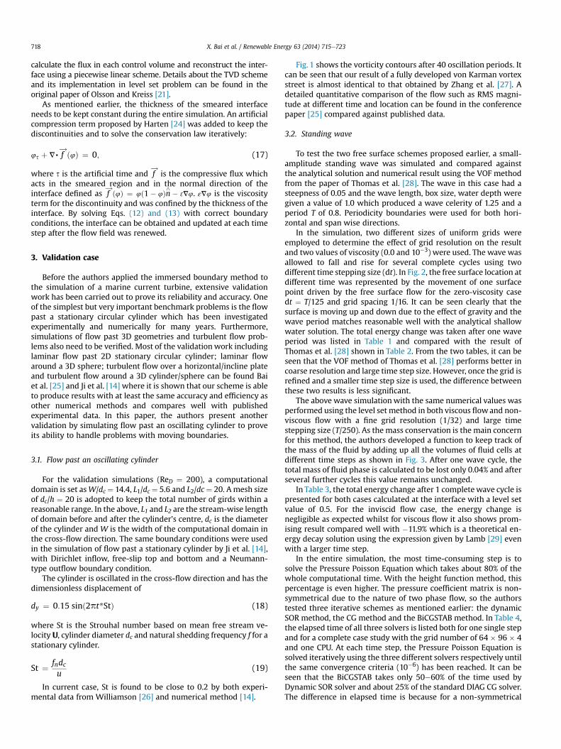
Fig. 1 shows the vorticity contours after 40 oscillation periods. Itcan be seen that our result of a fully developed von Karman vortexstreet is almost identical to that obtained by Zhang et al. [27]. Adetailed quantitative comparison of the flow such as RMS magni-tude at different time and location can be found in the conferencepaper [25] compared against published data.

3.2. Standing wave

To test the two free surface schemes proposed earlier, a small-amplitude standing wave was simulated and compared againstthe analytical solution and numerical result using the VOF methodfrom the paper of Thomas et al. [28]. The wave in this case had asteepness of 0.05 and the wave length, box size, water depth weregiven a value of 1.0 which produced a wave celerity of 1.25 and aperiod T of 0.8. Periodicity boundaries were used for both hori-zontal and span wise directions.

In the simulation, two different sizes of uniform grids wereemployed to determine the effect of grid resolution on the resultand two values of viscosity (0.0 and 10�3) were used. The wave wasallowed to fall and rise for several complete cycles using twodifferent time stepping size (dt). In Fig. 2, the free surface location atdifferent time was represented by the movement of one surfacepoint driven by the free surface flow for the zero-viscosity casedt ¼ T/125 and grid spacing 1/16. It can be seen clearly that thesurface is moving up and down due to the effect of gravity and thewave period matches reasonable well with the analytical shallowwater solution. The total energy change was taken after one waveperiod was listed in Table 1 and compared with the result ofThomas et al. [28] shown in Table 2. From the two tables, it can beseen that the VOF method of Thomas et al. [28] performs better incoarse resolution and large time step size. However, once the grid isrefined and a smaller time step size is used, the difference betweenthese two results is less significant.

The above wave simulationwith the same numerical values wasperformed using the level set method in both viscous flowand non-viscous flow with a fine grid resolution (1/32) and large timestepping size (T/250). As the mass conservation is the main concernfor this method, the authors developed a function to keep track ofthe mass of the fluid by adding up all the volumes of fluid cells atdifferent time steps as shown in Fig. 3. After one wave cycle, thetotal mass of fluid phase is calculated to be lost only 0.04% and afterseveral further cycles this value remains unchanged.

In Table 3, the total energy change after 1 completewave cycle ispresented for both cases calculated at the interface with a level setvalue of 0.5. For the inviscid flow case, the energy change isnegligible as expected whilst for viscous flow it also shows prom-ising result compared well with �11.9% which is a theoretical en-ergy decay solution using the expression given by Lamb [29] evenwith a larger time step.

In the entire simulation, the most time-consuming step is tosolve the Pressure Poisson Equation which takes about 80% of thewhole computational time. With the height function method, thispercentage is even higher. The pressure coefficient matrix is non-symmetrical due to the nature of two phase flow, so the authorstested three iterative schemes as mentioned earlier: the dynamicSOR method, the CG method and the BiCGSTAB method. In Table 4,the elapsed time of all three solvers is listed both for one single stepand for a complete case study with the grid number of 64 � 96 � 4and one CPU. At each time step, the Pressure Poisson Equation issolved iteratively using the three different solvers respectively untilthe same convergence criteria (10�6) has been reached. It can beseen that the BiCGSTAB takes only 50e60% of the time used byDynamic SOR solver and about 25% of the standard DIAG CG solver.The difference in elapsed time is because for a non-symmetrical

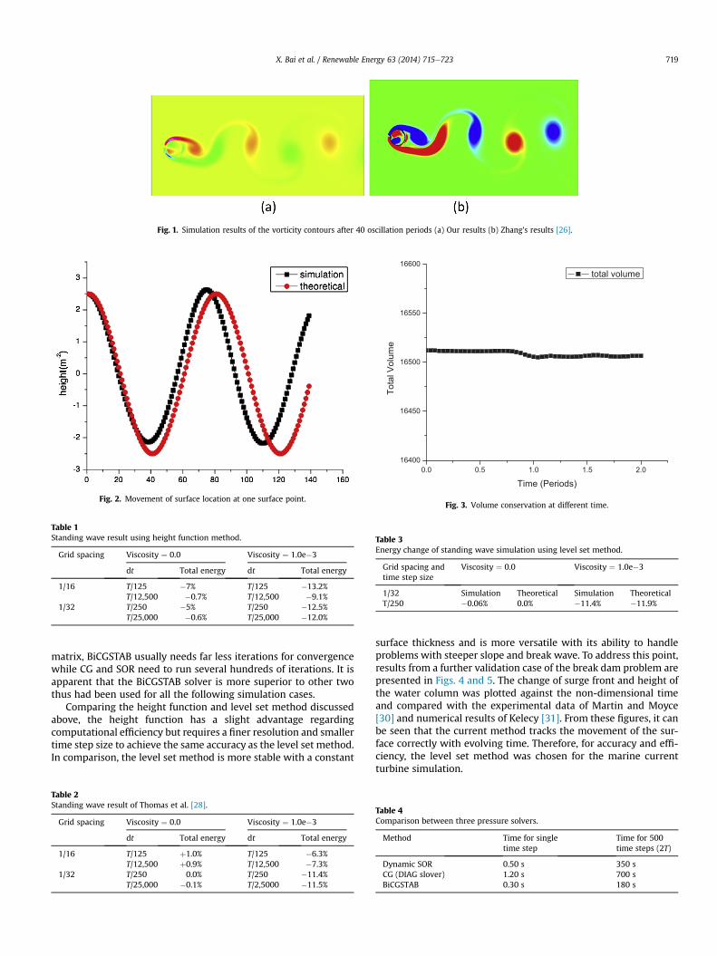
Fig. 1. Simulation results of the vorticity contours after 40 oscillation periods (a) Our results (b) Zhang’s results [26].

Fig. 2. Movement of surface location at one surface point.

Table 1Standing wave result using height function method.

Grid spacing Viscosity ¼ 0.0 Viscosity ¼ 1.0e�3

dt Total energy dt Total energy

1/16 T/125 �7% T/125 �13.2%T/12,500 �0.7% T/12,500 �9.1%

1/32 T/250 �5% T/250 �12.5%T/25,000 �0.6% T/25,000 �12.0%

0.0 0.5 1.0 1.5 2.016400

16450

16500

16550

16600

Tota

l Vol

ume

Time (Periods)

total volume

Fig. 3. Volume conservation at different time.

Table 3Energy change of standing wave simulation using level set method.

Grid spacing andtime step size

Viscosity ¼ 0.0 Viscosity ¼ 1.0e�3

1/32 Simulation Theoretical Simulation TheoreticalT/250 �0.06% 0.0% �11.4% �11.9%

X. Bai et al. / Renewable Energy 63 (2014) 715e723 719

matrix, BiCGSTAB usually needs far less iterations for convergencewhile CG and SOR need to run several hundreds of iterations. It isapparent that the BiCGSTAB solver is more superior to other twothus had been used for all the following simulation cases.

Comparing the height function and level set method discussedabove, the height function has a slight advantage regardingcomputational efficiency but requires a finer resolution and smallertime step size to achieve the same accuracy as the level set method.In comparison, the level set method is more stable with a constant

Table 2Standing wave result of Thomas et al. [28].

Grid spacing Viscosity ¼ 0.0 Viscosity ¼ 1.0e�3

dt Total energy dt Total energy

1/16 T/125 þ1.0% T/125 �6.3%T/12,500 þ0.9% T/12,500 �7.3%

1/32 T/250 0.0% T/250 �11.4%T/25,000 �0.1% T/2,5000 �11.5%

surface thickness and is more versatile with its ability to handleproblems with steeper slope and break wave. To address this point,results from a further validation case of the break dam problem arepresented in Figs. 4 and 5. The change of surge front and height ofthe water column was plotted against the non-dimensional timeand compared with the experimental data of Martin and Moyce[30] and numerical results of Kelecy [31]. From these figures, it canbe seen that the current method tracks the movement of the sur-face correctly with evolving time. Therefore, for accuracy and effi-ciency, the level set method was chosen for the marine currentturbine simulation.

Table 4Comparison between three pressure solvers.

Method Time for singletime step

Time for 500time steps (2T)

Dynamic SOR 0.50 s 350 sCG (DIAG slover) 1.20 s 700 sBiCGSTAB 0.30 s 180 s

Fig. 4. Surface profile at different time.

Table 5Blade profile specifications [7].

r/R r (mm) c/R Pitch (deg) Thickness/chord (%)

0.2 80 0.125 15 240.25 100 0.1203 12.1 22.50.3 120 0.1156 9.5 20.70.35 140 0.1109 7.6 19.50.4 160 0.1063 6.1 18.70.45 180 0.1016 4.9 18.10.5 200 0.0969 3.9 17.60.55 220 0.0922 3.1 17.10.6 240 0.0875 2.4 16.60.65 260 0.0828 1.9 16.10.7 280 0.0781 1.5 15.60.75 300 0.0734 1.2 15.10.8 320 0.0688 0.9 14.60.85 340 0.0641 0.6 14.10.9 360 0.0594 0.4 13.60.95 380 0.0547 0.2 13.11.0 400 0.05 0 12.6

X. Bai et al. / Renewable Energy 63 (2014) 715e723720

3.3. Simulation of the power performance of a rotating marinecurrent turbine

The turbine design of Bahaj et al. [7] was chosen for this project’svalidation purposes as large associated data-sets are available. Theselected model turbine has a diameter of 800 mm and consisted ofthree blades developed from the NACA 63-8XX series airfoil sec-tions. There are 17 stations along each blade of which the co-ordinates are interpolated from coordinate-based data for NACA63-812, 63-815, 63-818, 63-821 and 63-824. These simple profilesare given different thickness characteristics, chord length, and pitchdistributions to form a complicated 3D twisting blade. The detailedcharacteristics of each station can be found in Table 5.

Having known all the geometrical specifications, the turbinewas constructed using CAD tools and points were then taken fromthe exposed surfaces for the Immersed Boundary Points. Fig. 6

Fig. 5. Square dam break problem h ¼ 0.05175 m (a) surge front against non-

shows the visualisation of a marine turbine with a 20� hub pitchangle which was used in the following simulations. The main in-terest of the authors’ research was to predict the power perfor-mance of the turbine in a range of rotational speeds, flow speedsand different hub pitch angles. In the experiment of Bahaj et al. [7],the range of tip speed ratios (TSRs) required for this investigationwas achieved with a constant channel speed by varying the rotorrotational speed. The variation in rotor speed was achieved byvarying the load on the rheostats and in our numerical simulation,the same setting can be easily reproduced by fixing the rotatingspeed of the turbine to different prescribed values. The power co-efficient for each rotational speed can then be obtained using thefollowing equation,

CP ¼ QU12 rpR

2U3N

(20)

where R is the radius of the turbine, UN is the channel free streamvelocity, U is the rotational speed (rad/s) and Q is the torque on theblade which was produced by the fluid. The tip speed ratio (TSR) isdefined as TSR ¼ QU/UN.

Several small scale simulations have been performed using theturbine design above in a relatively smaller computation domain toprovide a quick preview of how the turbine works. Figs. 7 and 8

dimensional time (b) water column height against non-dimensional time.

Fig. 6. The visualisation of a marine turbine with a 20� hub pitch angle.

X. Bai et al. / Renewable Energy 63 (2014) 715e723 721

show the contour of the stream-wise flow velocity and isosurface ofthe vortex magnitude behind the rotating turbine in a laminar andturbulence flow respectively. It can be clearly seen that the im-mediate wake exists and a low velocity region follows the shape ofthe turbine. As the inflow speed increases, this region became lessclear due to the turbulence effects but is still noticeable. From thevortex contour, the turbine is rotating in anti-clockwise directionand has a strong vortex behind it. As the Reynolds number isincreased, this effect is further exaggerated.

For the main simulation the computational domain is set to 10Din the stream-wise directionwhereD is the diameter of the turbine.And the turbine is placed 3D from the inlet, the height is set to 3Dwith a blade tip immersion of 0.55D which is the same as theexperimental setting, the width of the domain is to set to 5D toeliminate the effect of the side-walls. To take advantage of theimmersed boundary method, a uniform rectangle grid was used forall simulations. The finest grid resolution was 1280 � 384 � 640 instream wise, vertical and span wise directions respectively,resulting in a total grid number of 300 million. The simulation wascarried out on UK high end parallel computer HECToR using a totalof 150 CPUs.

Fig. 7. At ReD ¼ 1e þ 3 the contour of stream-wise flow

Inflow and outflow boundary conditions are used and the freesurface was initialized as a flat surface tracked by the level setmethod, the bottom was set to a free-slip wall and a periodicboundary condition is used for the sidewalls. The simulationwas tobe carried out by setting the hub pitch angle to 20� and the inflowspeed of 1.73m/s to produce a curve of the power coefficient versusdifferent TSR speeds in the turbulent flow. Based on the rotordiameter, the Reynolds number for this simulation can be calcu-lated as:

ReD ¼ rDUN

m¼ 1000kg=m3*0:8m*1:73m=s

1:002*10�3Pa s¼ 1:38� 106

(21)

where m is the dynamic viscosity for water at 20 �C.The main simulation in the full scale computational domain

mentioned abovewas then carried out to predict the hydrodynamicperformance of themarine turbine and also served as a validation ofour numerical code. In Fig. 9, the power coefficient at three differentTSR speedswas plotted and comparedwith the experimental data ofBahaj et al. [7]. Our results follow closely the trend of the powercurve and the experimental data: as the rotation speed increases,the power coefficient first increases and then decreases afterreaching itsmaximum. This can be used to determine the optimizedoperation speed of the turbine if installed in a locationwith certainrange of flow speed. In our case, the TSR for the maximum powerexploitation should be close to 6 as shown in Fig. 9. The influence ofgrid resolution on this strongly coupled fluid-solid interactionproblem has been investigated and an increased accuracy can beobserved in Fig. 9 with half the grid size but the same model size. Itcan be seen that the case with refined grid shows a better matchwith the experimental data and has an error range of about 4%. Also,the existence of the free surface has caused a slight increase in thepower coefficient although there is no significant deformationobserved throughout the simulation. It is reasonable to believe thatthe increasewill bemuchhigher if the turbine is located closer to thesurface orwith a surfacewave. The deviation from the experimentalcurve can be due to several aspects: domain size, the number ofpoints used to represent the body, or the grid resolution. Because thesimulation is run on a structured grid, for a 3D problemdoubling thegrid resolution means the overall computational cost is 16 timesgreater than before due to de decrease of the time step. For coarsegrid, there are only 2e3 cells along the vertical direction and 4e6cells in stream-wise at the blade tip where the rotation speed is the

velocity (a) and isosurface of vortex magnitude (b).

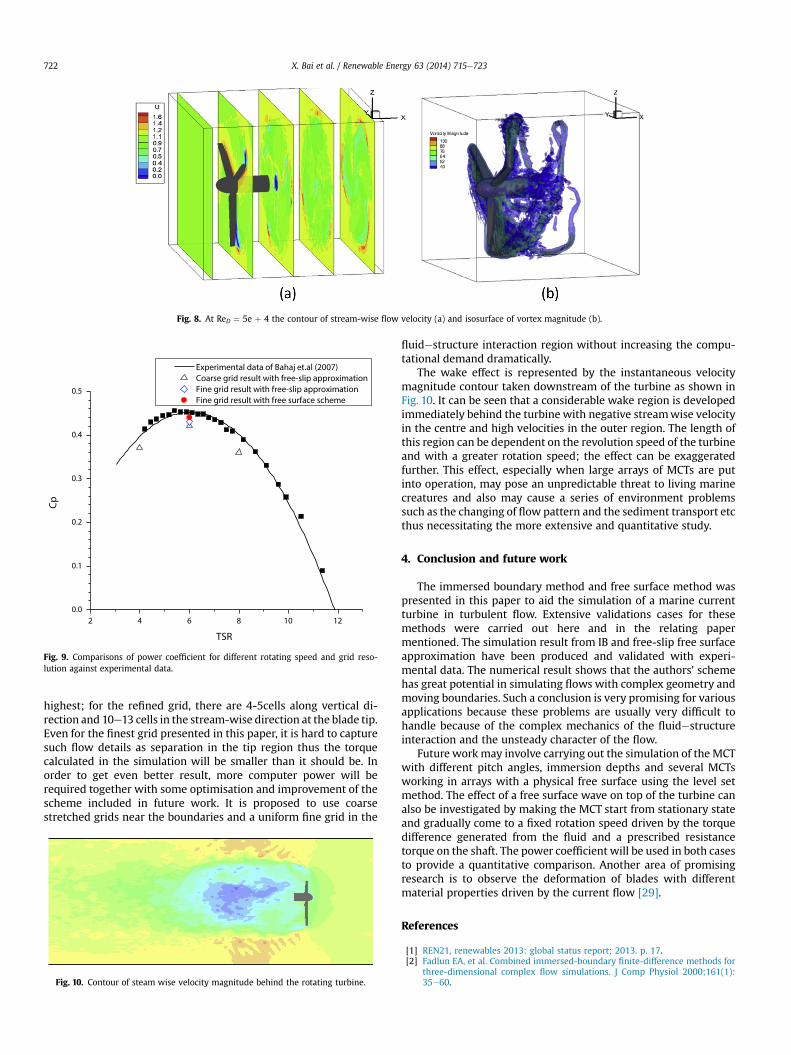
Fig. 8. At ReD ¼ 5e þ 4 the contour of stream-wise flow velocity (a) and isosurface of vortex magnitude (b).

Fig. 9. Comparisons of power coefficient for different rotating speed and grid reso-lution against experimental data.

X. Bai et al. / Renewable Energy 63 (2014) 715e723722

highest; for the refined grid, there are 4-5cells along vertical di-rection and 10e13 cells in the stream-wise direction at the blade tip.Even for the finest grid presented in this paper, it is hard to capturesuch flow details as separation in the tip region thus the torquecalculated in the simulation will be smaller than it should be. Inorder to get even better result, more computer power will berequired together with some optimisation and improvement of thescheme included in future work. It is proposed to use coarsestretched grids near the boundaries and a uniform fine grid in the

Fig. 10. Contour of steam wise velocity magnitude behind the rotating turbine.

fluidestructure interaction region without increasing the compu-tational demand dramatically.

The wake effect is represented by the instantaneous velocitymagnitude contour taken downstream of the turbine as shown inFig. 10. It can be seen that a considerable wake region is developedimmediately behind the turbine with negative streamwise velocityin the centre and high velocities in the outer region. The length ofthis region can be dependent on the revolution speed of the turbineand with a greater rotation speed; the effect can be exaggeratedfurther. This effect, especially when large arrays of MCTs are putinto operation, may pose an unpredictable threat to living marinecreatures and also may cause a series of environment problemssuch as the changing of flow pattern and the sediment transport etcthus necessitating the more extensive and quantitative study.

4. Conclusion and future work

The immersed boundary method and free surface method waspresented in this paper to aid the simulation of a marine currentturbine in turbulent flow. Extensive validations cases for thesemethods were carried out here and in the relating papermentioned. The simulation result from IB and free-slip free surfaceapproximation have been produced and validated with experi-mental data. The numerical result shows that the authors’ schemehas great potential in simulating flows with complex geometry andmoving boundaries. Such a conclusion is very promising for variousapplications because these problems are usually very difficult tohandle because of the complex mechanics of the fluidestructureinteraction and the unsteady character of the flow.

Future work may involve carrying out the simulation of the MCTwith different pitch angles, immersion depths and several MCTsworking in arrays with a physical free surface using the level setmethod. The effect of a free surface wave on top of the turbine canalso be investigated by making the MCT start from stationary stateand gradually come to a fixed rotation speed driven by the torquedifference generated from the fluid and a prescribed resistancetorque on the shaft. The power coefficient will be used in both casesto provide a quantitative comparison. Another area of promisingresearch is to observe the deformation of blades with differentmaterial properties driven by the current flow [29].

References

[1] REN21, renewables 2013: global status report; 2013. p. 17.[2] Fadlun EA, et al. Combined immersed-boundary finite-difference methods for

three-dimensional complex flow simulations. J Comp Physiol 2000;161(1):35e60.

X. Bai et al. / Renewable Energy 63 (2014) 715e723 723

[3] Wave energy project results: the exploitation of tidal marine currents. Com-mission of the European Communities; 1996.

[4] 2010; Available from: www.dti.gov.uk/energy/inform/energy_stats/.[5] Consul CA, Willden RHJ, McIntosh SC. Blockage effects on the hydrodynamic

performance of a marine cross-flow turbine. Philosophical Trans R Soc A-MathPhys Eng Sci 2013;371(1985).

[6] Kinnas, Xu. Analysis of tidal turbines with various numerical methods. In: 1stannual MREC technical conference 2009. Massachusetts, USA.

[7] Bahaj AS, et al. Power and thrust measurements of marine current turbinesunder various hydrodynamic flow conditions in a cavitation tunnel and atowing tank. Renew Energy 2007;32(3):407e26.

[8] Buhl WT. Perf user’s guide. National Renewable Energy Laboratory; 2009.[9] Peskin HM. National accounting and the environment. Artikler fra Statistisk

sentralbyrå, nr 50. Oslo: Aschehoug; 1972. p. 60.[10] Mohd-Yusof J. Combined immersed-boundary/B-spline methods for simula-

tions offlow in complex geometries. In: Annual researchbriefs 1997. p. 317e27.[11] Verzicco R, et al. Large eddy simulation in complex geometric configurations

using boundary body forces. Aiaa J 2000;38(3):427e33.[12] Uhlmann M. An immersed boundary method with direct forcing for the

simulation of particulate flows. J Comp Physiol 2005;209(2):448e76.[13] Thomas TG, Williams JJR. Development of a parallel code to simulate skewed

flow over a bluff body. J Wind Eng Ind Aerodynam 1997;67e68:155e67.[14] Ji C,MunjizaA,Williams JJR.Anovel iterativedirect-forcing immersedboundary

method and its nite volume applications. J Comp Physiol 2012;231(4):25.[15] Barltrop N, et al. Investigation into wave-current interactions in marine cur-

rent turbines. Proc Inst Mech Eng Part A-J Pow Energy 2007;221(A2):233e42.[16] Nichols BD, Hirt CW. Calculating 3-dimensional free-surface flows in vicinity

of submerged and exposed structures. J Comp Physiol 1973;12(2):234e46.[17] Harlow FH, Welch JE. Numerical calculation of time-dependent viscous

incompressible flow. Phys Fluids 1965;8.[18] Bornia G, et al. On the properties and limitations of the height function

method in two-dimensional Cartesian geometry. J Comp Physiol 2011;230(4):851e62.

[19] Osher S, Sethian JA. Fronts propagating with curvature-dependent speedealgorithms based on Hamilton-Jacobi formulations. J Comp Physiol1988;79(1):12e49.

[20] van der Pijl SP, et al. A mass-conserving level-set method for modelling ofmulti-phase flows. Int J Numer Meth Fluids 2005;47(4):339e61.

[21] Sussman M, Fatemi E. An efficient, interface-preserving level set redistancingalgorithm and its application to interfacial incompressible fluid flow. Siam JScientific Comput 1998;20(4):1165e91.

[22] Olsson E, Kreiss G. A conservative level set method for two phase flow. J CompPhysiol 2005;210(1):225e46.

[23] LeVeque RJ. Finite volume methods for hyperbolic problemsIn Cambridgetexts in applied mathematics, vol. xix. Cambridge ; New York: CambridgeUniversity Press; 2002. p. 558.

[24] Harten A. The artificial compression method for computation of shocks andcontact discontinuities. Comm Pure Appl Math 1977:611e38.

[25] X.Bai, Avital EJ, Williams JJR. Numerical simulation of a marine current turbinein turbulent flow. In: 6th international conference on energy & development,environment & biomedicine (EDEB’12). Athens, Greece: Vouliagmeni Beach;2012.

[26] Williamson CHK. Oblique and parallel modes of vortex shedding in thewake of a circular-cylinder at low Reynolds-numbers. J Fluid Mech1989;206:579e627.

[27] Zhang N, Zheng ZC. An improved direct-forcing immersed-boundary methodfor finite difference applications. J Comp Physiol 2007;221(1):250e68.

[28] Thomas TG, Leslie DC, Williams JJR. Free-surface simulations using a conser-vative 3d code. J Comp Physiol 1995;116(1):52e68.

[29] Lamb H. Hydrodynamics. 6th ed., vol. 2. New York: Dover publications; 1945l.viiexv, 738 p.

[30] Martin JC, Moyce WJ. An experimental study of the collapse of liquid columnson a 331 rigid horizontal plane. Philos T R Soc 1952;224:13.

[31] Kelecy FJ, Pletcher RH. The development of a free surface capturing approachfor multidimensional free surface flows in closed containers. J Comp Physiol1997;138(2):939e80.