Numerical simulation and performance assessment of an absorption solar air-conditioning system...

Research Article

Building Systems and

Components

E-mail: [email protected]

Numerical simulation and performance assessment of an absorption solar air-conditioning system coupled with an office building

Sébastien Thomas (), Philippe André

Department of Sciences and Environmental Management, University of Liège, 185 Avenue de Longwy, 6700 Arlon, Belgium Abstract To minimize environmental impact and CO2 production associated with air-conditioning, it is reasonable to evaluate the prospects of a clean energy source. Solar energy, via thermal collectors can provide a part of the heating needs. Moreover, it can drive absorption chiller in order to satisfy the cooling needs of buildings. The objective of the work is to evaluate accurately the energy consumption of an air-conditioning system including a solar driven absorption chiller. The complete simulation environment includes the absorption chiller itself, the cooling tower, the solar collectors field, heater, storage devices, pumps, heating-cooling distribution, emission system and building. A decrease of primary energy consumption of 22% for heating and cooling is reached when using a solar air-conditioning system instead of classical heating and cooling devices. The modelling of each subsystem is detailed. TRNSYS software modular approach provides the possibility to model and simulate this complete system.

Keywords TRNSYS,

solar cooling,

absorption Article History Received: 4 August 2011

Revised: 5 December 2011

Accepted: 8 December 2011 © Tsinghua University Press and

Springer-Verlag Berlin Heidelberg

2012

1 Introduction

Solar air-conditioning is a good way to use renewable energy instead of fossil fuels to meet heating and cooling needs of buildings. It implies a decrease in energy consumption and CO2 rejection. There were in year 2010 around 600 identified systems in operation all over the world while around 500 were located in Europe (Jakob 2011). A lack of awareness of such technologies is still encountered. The development of solar air-conditioning (SAC) technology is closely linked to its economical profitability. To check what the real benefits of SAC installation are, it is important to compute the energy savings as well as their essentials parameters (Casals 2006).

Previous work (Barbosa and Mendes 2008) about analysis of heating and cooling consumption suggests considering an integral approach to evaluate energy savings. Moreover, performance is greatly depending on external conditions and on cooling load dynamics in SAC systems (Bujedo et al. 2008). It is thus important to think about the whole system (Mugnier 2002; Eicker and Pietruschka 2009).

This study concerns a common solar air-conditioning system. A solar collector field provides hot water to a storage

tank. Hot water then can be used for heating the building or feeding an absorption machine. This last device is used to produce cold water (Herold et al. 1996). As solar energy is not enough to heat and cool the whole building through the year, back up systems are used. To heat, a conventional gas boiler is used. To cool, two choices of back up can be assessed: heating water to feed the absorption chiller or use of a classical vapour compression chiller (electricity driven). A previous work (Thomas and André 2009a) has pointed out that the second choice is the best one from a primary energy point of view; it will be implemented in this study. The two choices mentioned here above can be roughly summarized as follows. The gas boiler back up namely “hot back up” produces generally 0.63 kWhcold with 1 kWhprim (boiler yield 0.9 multiplied by absorption chiller thermal COP 0.7) while the vapour compression chiller “cold back up” produces commonly 1.12 kWhcold with 1 kWhprim (primary energy factor for electricity 1/2.5 multiplied by the vapour compression chiller electrical COP 2.8).

A complete simulation environment is presented in this paper, it is implemented in TRNSYS (2006). Generally, the analysis is focused on the basic heating and cooling load of the building. Here, numerous other devices and effects are

BUILD SIMUL (2012) 5: 243–255 DOI 10.1007/s12273-012-0060-0

Thomas and André / Building Simulation / Vol. 5, No. 3

244

List of symbols

ABS absorption chiller COP thermal coefficient of performance COPelec electrical coefficient of performance cp heat capacity (J/(kg·K)) ETC evacuated tube collector FCU fan coil unit fnc absorption chiller fraction of nominal capacity fdei absorption chiller fraction of design energy input SF solar fraction Q power of the thermal energy flow (kW) U wall thermal conductivity (W/(m2 ·K))

VCC vapour compression chiller λ material thermal conductivity (W/(m·K)) ρ density (kg/m3)

Subscripts

cold cold water (to cool the building) hot hot water (from hot water storage) prim primary energy nom nominal rated rated conditions coll collector

modelled and connected together: Building

Internal gains, light dimming, moveable solar protections, latent loads

Hot and cold distribution and emission Fan coil units, pumps, pipes

Hot and cold production and storage Gas boiler, solar loop, hot water storage, absorption chiller, cooling tower, vapour compression chiller (for back up only).

Climate These four subsystems constitute the simulation environ-

ment layers detailed in Fig. 1. This kind of implementation gives the opportunity to analyse relations between the absorption chiller and the building. Moreover, the modularity of this approach is suitable with model switching. The different layers modelling and simulation are described

Fig. 1 Simulation layers

in the next sections. In order to easily compare energy consumptions, a reference case called “classical air- conditioning” is defined. It includes an electricity driven vapour compression chiller for cold production and a boiler for heating but neither solar panels nor storage devices. Comparison is done on the net energy consumption and on the primary energy consumption. The assessment deals also with the electricity consumption of lighting system, appliances and ventilation system. In this way the global energy use of the building is considered.

2 Building modelling

The analysis deals with a theoretical building representative of existing large office buildings in Europe. It was defined by Stabat (2007) in the frame of the IEA-ECBCS annex 48 project called Heating Pumping and Reversible Air Con- ditioning. It is a twelve identical floors, 15 000 m2 building with an average of 1000 persons occupancy. From the modelling point of view, only one floor is modelled but all the floors can be treated similarly. A three-floor building is considered for the solar collector field design (see Section 4.4).

2.1 Geometrical description

Geometrical description is presented in Fig. 2. Five zones are considered for a total of 1250 m2.

Fig. 2 Typical floor for an office building (Stabat 2007)


245

2.2 Envelope

The building studied is representative of existing buildings, the insulation is thus not very efficient. North and south facade are similarly largely glazed while east and western are blind walls. Rooms are 3 m high while windows take up 2 m. Wall constitution and U values are described in Table 1.

2.3 Internal heat gains

People

Offices and conference room have two different schedules and occupancy rate. The sizing of the offices is defined as one person per 12 m2 (1 person per 3.5 m2 for conference room). The sensible heat released by each person is supposed to be 105 W and the moisture release is 0.09 kg/h (Stabat 2007). Occupancy profile are defined in Fig. 3. The ratio is the current occupancy divided by the sizing value. No consideration about holiday is taken into account. During weekend, appliances gains as well as occupancy are null.

Appliances

Similarly to previous paragraph, appliances gains are defined. Figure 3 notifies that the appliances ratio for a sizing value is 15 W/m2. The appliances are essentially computers; these gains exist only in the offices zones.

Lighting system

The lighting power is set to 18 W/m2 in offices and conference rooms, 12 W/m2 in the circulations and 6 W/m2 in the toilets. Based on the work of Alessandrini et al. (2006) the use of artificial lighting depends on natural light available for

workers. Between 0 and 100 lx, the use of artificial lighting is 90%; between 100 and 700 lx, it drops linearly to 30%; it falls to 0% when the available natural light is higher than 2500 lx. The available light is computed with TRNSYS regarding the solar energy through the windows. A basic law is implemented and considers whole solar radiation spectrum as visible light. Lights are switched on only during occupancy, in toilets and circulation zone it is always on from 6 a.m. to 7 p.m.

2.4 Solar protections

Manual external solar protections are modelled. They implement the behaviour of the people in the zones (Allessandrini 2006). When the solar protections are completely closed, the energy transmission is 20%. The use opening of solar protections is achieved by the user; depending on the outside luminance, the solar protections are closed from 7% to 45%. The position of solar protections during non occupancy is defined as equal to those in the last hour of occupancy.

2.5 Ventilation and infiltration

Constant mass flow is blown in the building during occupancy (Fig. 4), it corresponds to 25 m3/h fresh air per person for offices and 30 m3/h per person for conference room. No heat recovery is implemented. When there is no occupancy, the mechanical ventilation is switched off; infiltration is then equal to 0.373 volume per hour. For all zones except conference room the power of ventilator is 330 W (single flux ventilation). For conference room, a double flux ventilation without recovery is implemented, it leads to fan power 2 times 470 W (0.21 W/(m3·h)).

Table 1 Wall constitution

Constitution U value (W/(m2·K))

Outside wall

Outside layer: cement 0.13 m ( 1900 kg/m3, 0.58 W/(m·K), cp 1000 J/(kg·K)) Insulating material 0.024 m ( 56 kg/m3, 0.029 W/(m·K), cp 1220 J/(kg·K)) Inside layer: plaster 0.012 m ( 1860 kg/m3, 0.72 W/(m·K), cp 840 J/(kg·K))

0.8

Windows Double glazing of 0.004 m width for each glazing and 0.008 m air space. 2.95

Floor & ceiling Cement 0.1 m ( 1900 kg/m3, 0.58 W/(m·K), cp 1000 J/(kg·K)) 5.8

Roof

Outside layer: cement 0.13 m ( 1900 kg/m3, 0.58 W/(m·K), cp 1000 J/(kg·K)) Insulating material 0.06 m ( 56 kg/m3, 0.029 W/(m·K), cp 1220 J/(kg·K)) Inside layer: plaster 0.012 m ( 1860 kg/m3, 0.72 W/(m·K), cp 840 J/(kg·K))

0.4

Inner walls Plaster 0.02 m ( 1860 kg/m3, 0.72 W/(m·K), cp 840 J/(kg·K)) 36


246

Fig. 3 Schedules for occupancy and appliances (Stabat 2007)

Fig. 4 Ventilation mass flows for one floor

2.6 Temperature and humidity set points

The set points for heating are 21℃–40% relative humidity in all heated zones (offices and conference room) during occupancy period. All over the year, the minimal temperature in those zones is 15℃. For cooling, the set point is 24℃–60% relative humidity during occupancy. According to the DIN 1946 German regulation, a 26℃ room air temperature is acceptable for people. If external temperature is greater than 29℃, a higher internal temperature is comfortable. There is no upper limit zone temperature for other periods. Two simulations are run, one with the common temperature set point (24℃) and the other one with DIN 1946 regulation (26℃).

3 H&C emission and distribution

This part focuses on the heat and cold emission and distribution layer of a common office building. It does not integrate any devices facilitating implementation of solar air-conditioning (e.g., cooling ceiling). Links with other layers are drawn in Fig. 1 whereas the implementation of this layer is described in Fig. 5. The TRNSYS types numbers are also mentioned. In the building analyzed, heating and cooling loads are sometimes simultaneous. Heating and cooling

Fig. 5 Emission distribution network implementation scheme

systems have their own pipe network. The links with building layer consist in heating and cooling sensible and latent energy given in each room by the fan coil units (FCU) and the pipe losses. The temperature of each room acts as an input for FCU control. The links with production layer are the temperature and the mass flow for each network.

3.1 Pipes

As described in literature (Stabat 2007), the hot or cold network is summed up into two pipes (one supply, one return) with a total length of 65 m each. Their losses are 0.28 W/K for each pipe meter. Losses to the ambient (22℃ all over the year) are 80% recovered by the building.

3.2 Pumps

Pressure drop, pump efficiency (40%) and mass flow (depending on the number of fan coil units and their characteristics) are defined. The power of the heat network pump is 475 W while that of the cold pump is 1485 W. The first pump is in operation only when there are heating needs while the second is permanently ON. Moreover, the entire pump power is transferred to fluid.

3.3 Fan coil units (FCU)

The heating-cooling coils are effectively transferring heat–cold to the building. The control is achieved by a valve adjusting the mass flow in order to satisfy the room temperature set point. In order to model as accurately as possible the heat–cold emission, it has been decided to create a new fan coil model with behaviour as close as possible to the manufacturer data (we suppose it is closed to the reality). To achieve this, it is common to evaluate a polynomial estimation of the real behaviour (Barbosa and Mendes 2008). The chosen fan coil (CARRIER 2007) nominal characteristics


247

are specified in Table 2. The objective of the FCU model is to evaluate the heat or cold provided by the coil according to some variables. These are different for heating and cooling: for heating coil, sensible heat depends on the water mass flow and the difference between water inlet temperature and room dry bulb temperature; for the cooling coil, sensible cooling load depends on the cooling coil entering temperature and the room temperature. Normally the temperature gap between supply and return cold water should be taken into account but this involved convergence issues.

The sensible heating power according to mass flow and temperature gap between water supply temperature and room air temperature is presented in Fig. 6. Polynomial approximation computed with Matlab (Matlab 2007) gives a mean error of 0.9% when evaluating the whole operating points given by the manufacturer.

Other coil models have been tested: Some of the existing models of heating cooling coil in

TRNSYS are tuned with only one parameter: heat exchanger efficiency or bypass air fraction (Klein 2007). These models are not accurate for the whole range of FCU use (16.5% mean error for Type 670—10.2% for type 753).

Other models read manufacturer data in an external file (e.g., type 697b). This is a good way to have the real behaviour of a fan coil. However, it requires translating all the working points to a suitable file format (this can be source of numerous errors).

Table 2 Fan coil characteristics for 42N60 model (nominal operation—centrifugal fan at high speed)

Heating Cooling

Water mass flow 0.25 kg/s 0.23 kg/s

Dry bulb air temp. T 27℃

Supply water temp. T + 60℃ 7℃

Return temp. — 12℃

Sensible capacity 8400W 4880 W

Fig. 6 Polynomial approximation of FCU power (where ΔT = Twater supply – Troom)

The total number of fan coils has been chosen based on the highest cooling or heating loads and on FCU power at nominal capacity. This gives 25 FCU for the entire floor. They are distributed into the three zones: 7 for offices south, 11 for offices north, 7 for conference room. All the FCU of the same zone are controlled similarly.

Fan power is 113 W per FCU. It is switched on only when there is heating or cooling load in the zone.

Latent load is not handled by the model presented in this paragraph because of the lack of manufacturer data. Nevertheless, it is taken into account in the water loops. Latent load computed by TRNSYS building model to maintain the set point is translated into a temperature difference in water flow before the return pipe. This is a very simple way to treat this load but it counts for around only 10% of the total cooling load. A future better FCU model should handle the latent load.

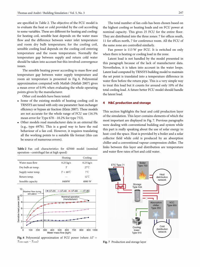
4 H&C production and storage

This section highlights the heat and cold production layer of the simulation. This layer contains elements of which the most important are displayed in Fig. 7. Previous paragraphs were dealing with conventional building and system while this part is really speaking about the use of solar energy to heat–cool the space. Heat is provided by a boiler and a solar collector field while cold is produced by an absorption chiller and a conventional vapour compression chiller. The links between this layer and distribution are temperature and water flow rates of hot and cold water.

Fig. 7 Production and storage layer


248

4.1 Absorption chiller

The heat provided by solar collectors is stored and feeds an absorption chiller to produce cold water. Among all kind of thermally driven chiller available on the market, a lithium bromide–water absorption chiller was chosen. This type of machine is mostly used in offices solar air-conditioning systems (Sparber and Napolitano 2009).

Absorption chiller behaviour has been implemented in a new TRNSYS Type 255 (nearly the same as existing TRNSYS Type 107) based on manufacturer curves (YAZAKI 2008) of a 105 kWcold absorption chiller (COPrated = 0.695). It is fitted to the modelled floor cooling demand.

The existing model (Type 107) is modelling the energy balance, but not the chiller inertia nor other dynamic effects. Absorption chiller works with three energy flows: high temperature flow (>70℃) drives the machine; cold flow (7–12℃) satisfies the building cooling load; rejection flow at medium temperature (35–40℃) is rejected to the atmosphere.

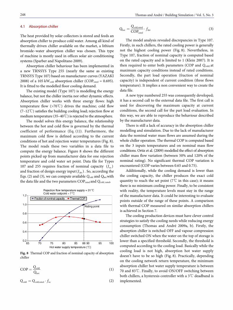
The model solves this energy balance, the relationship between the hot and cold flow is governed by the thermal coefficient of performance (Eq. (1)). Furthermore, the maximum cold flow is defined according to the current conditions of hot and rejection water temperatures (Fig. 8). The model reads these two variables in a data file to compute the energy balance. Figure 8 shows the different points picked up from manufacturer data for one rejection temperature and cold water set point. Data file for Types 107 and 255 requires fraction of nominal capacity nc( )J and fraction of design energy input dei( )J . So, according the Eqs. (2) and (3), we can compute available Qcold and Qhot with the data file and the two parameters COPrated and Qcold, rated.

Fig. 8 Thermal COP and fraction of nominal capacity of absorption chiller

cold

hotCOP Q

Q= (1)

cold cold,rated ncQ Q f= ⋅ (2)

cold,ratedhot dei

ratedCOPQQ f= ⋅ (3)

The model analysis revealed discrepancies in Type 107. Firstly, in such chillers, the rated cooling power is generally not the highest cooling power (Fig. 8). Nevertheless, in Type 107, fraction of nominal capacity is computed based on the rated capacity and is limited to 1 (Klein 2007). It is then required to enter both parameters (COP and Qcold) at maximum capacity conditions instead of rated conditions. Secondly, the part load operation (fraction of nominal capacity) is independent of current condition (three flows temperature). It implies a non convenient way to create the data file.

A new type numbered 255 was consequently developed; it has a second call to the external data file. The first call is used for discovering the maximum capacity at current conditions, the second call for the part load evaluation. In this way, we are able to reproduce the behaviour described by the manufacturer data.

There is still a lack of accuracy in the absorption chiller modelling and simulation. Due to the lack of manufacturer data the nominal water mass flows are assumed during the whole chiller operation. The thermal COP is computed based on the 3 inputs temperatures and on nominal mass flow conditions. Ortiz et al. (2009) modelled the effect of absorption chiller mass flow variation (between 50% and 120% of the nominal rating). No significant thermal COP variation is encountered (COP varies between 0.65 and 0.75).

Additionally, while the cooling demand is lower than the cooling capacity, the chiller produces the exact cold quantity to reach the set point (7℃ in this case); it means there is no minimum cooling power. Finally, to be consistent with reality, the temperature levels must stay in the range of the manufacturer data. It could be interesting to evaluate points outside of the range of these points. A comparison with thermal COP measured on similar absorption chillers is achieved in Section 7.

The cooling production devices must have clever control strategies to satisfy the cooling needs while reducing energy consumption (Thomas and André 2009a, b). Firstly, the absorption chiller is switched OFF and vapour compression chiller switched ON when the water on the top of storage is lower than a specified threshold. Secondly, the threshold is computed according to the cooling load. Basically while the cooling load is not high, absorption hot water supply doesn’t have to be so high (Fig. 8). Practically, depending on the cooling network return temperature, the minimum absorption chiller hot water supply temperature is between 70 and 83℃. Finally, to avoid ON/OFF switching between both chillers, a hysteresis controller with a 3℃ deadband is implemented.


249

4.2 Heat storage

The fundamental element of the production storage layer is the storage tank (TRNSYS Type 534); as shown in Fig. 7, three circuits are directly connected to it (no heat exchanger in the tank): solar collector, building heating network and absorption chiller hot water loop. The solar radiation is the only energy source supplying heat to the tank. A 0.2 m thick rock wool insulation has been modelled in order to decrease storage losses. Storage tank volume is 7 m3, which is optimized for this application.

4.3 Cooling tower

The absorption chiller needs a rejection circuit to evacuate both energy flows (energy from collectors and from building). Heat rejection control is crucial to guarantee good perfor- mances of absorption chiller. The model used is Type 510 representing a closed cooling tower. According to the authors (Zweifel at al. 1995) it is able to find accurately the power rejected based on only one design point. This point has been found for an existing machine (AEC 2007) with a nominal rejection power of 263 kW.

Control of outlet water temperature is done by modifying the cooling tower fan speed. Assumption done here is that fan speed varies continuously from zero (when inlet temperature is 27℃) to its nominal power 3.7 kW (when inlet temperature is 35℃). In this way a low cooling tower return temperature (below 30℃) can be achieved all over the year.

4.4 Solar collector field

Evacuated tube collectors (ETC) are used because of the slightly high temperature they can reach. In comparison with commonly used flat plat collector, those collectors have a better yield in the absorption chiller operating temperature range (70–95℃). Some of the installed absorption solar air-conditioning systems are nevertheless using flat plat collectors (Sparber and Napolitano 2009) mainly for economical reasons. Type 71 has been chosen to implement the manufacturer data (SCHOTT 2003) including collector yield, incidence angle modifier and mass flow variation. Rules must be defined to size the collector field. The following hypothesis is selected for this study: the only available space is the flat roof of the building. A three floor building is then considered instead of twelve mentioned in Section 2. It leads to an available solar absorption area of 142 m2 per floor. Moreover, optimisation finds the best design of the collector field: four rows with 15° slope and obviously oriented south. The size of the collector field clearly influences the solar fraction. Hypothesis selected in this

work lead to the value of around 2.5 m2 collector area per kWcold nominal load (50 kW see Fig. 14 Section 6.3). It is the average value of the installed solar-air conditioning systems (Henning 2007).

Shading is taken into account between rows by using a special model (Type 551). Finally, the solar loop is connected to the storage tank via a heat exchanger with 95% constant effectiveness. The mass flow from collectors has been set to 30 kg/h per collector area (Eicker and Pietruschka 2009).

4.5 Auxiliary gas boiler

A gas boiler is used as backup when the storage tank top temperature is lower than the temperature given by the heating curve (Fig. 9). The gas boiler performance is defined (Stabat 2007): yield at 100 % load is 89.2%; yield at 30% load is 88.2%; losses at 0% load are 1.3 kW. Interpolation is done between these three points. Rated power is 150 kW according to the maximal floor heating load. This device is switched OFF if there is no heating demand.

4.6 Vapour compression chiller

As mentioned in the introduction, the back-up system for cooling is a classical vapour compression chiller. In the frame of IEA ECBCS a reversible air cooled heat pump (WESPER 2005) was implemented into TRNSYS. The model consists in reading the manufacturer performance curves. This machine is exploited in this work to produce cold water at 7℃. Vapour compression chiller has 105 kWcold power, its seasonal COPelec is 3.5 (including fans and pumps).

4.7 Solar air-conditioning additional auxiliaries

The electricity consumption of the auxiliaries dedicated to solar air-conditioning system are evaluated. For the pumps, no typical pressure drops values are found for the different

Fig. 9 Boiler outlet water temperature set point (Stabat 2007)


250

circuits, pumps are not modelled as they were for distribution emission layer. Common energy consumption values are considered (Henning 2008): 0.02 kWh electricity per kWh thermal energy for the solar

system, 0.03 kWh electricity per kWh thermal energy for the heat

rejection, 0.01 kWh electricity per kWh thermal energy for the

absorption chiller. These values include pumps consumptions and other

auxiliaries such as cooling tower fans.

5 Climate

TRNSYS software makes the link between the building and the meteorological data. The Paris Montsouris station is selected to run simulations. The common format “Typical Meteorological Year” (TMY2) is used. It includes dry bulb temperature, relative humidity, solar diffuse and global radiation, sun position … Paris climate is warm temperate, the monthly mean temperature and total solar radiation on horizontal are plotted on the Fig. 10.

Fig. 10 Paris TMY 2 data (yearly radiation on horizontal is 1036 kWh/m2)

6 Results

The building and HVAC devices presented below are simulated with TRNSYS using a 10 minutes time step. The simulation gives the opportunity to evaluate the energy consumption of the building. The results are presented and analyzed below. Three different time scales are considered for the heating and cooling consumption. The auxiliaries such as lighting, appliances and fans are treated separately (Section 6.4). Comparison is achieved with a classical solar air-conditioning. Primary energy consumption is sometimes mentioned. To convert net energy (energy you pay to your energy supplier) to primary energy, multiplication factor is 2.5 for electricity, 1 for gas (Belgian values). These conversion factors depend on the country. For Germany it

is 2.6 for electricity and 1.1 for natural gas (Kagerer and Herkel 2010) but mean European mix is 2.5 for electricity (Thür et al. 2010).

6.1 Yearly results

Global results about building energy consumption for heating and cooling are presented below. Various energy flows are integrated all over the year and are presented in kWh per building internal area per year (Fig. 11): boiler energy, vapour compression chiller (VCC). These first results focus on net energy for heating and cooling with the 21–24℃ set points. As mentioned in the previous section, solar energy is used both for heating and cooling. With solar air-conditioning (SAC), there is a decrease of 22% of the energy consumption while net energy for cooling drops off 40%. This last part has only a small impact on total building energy utilization. SAC implies additional electricity consumption (“solar auxiliaries electricity”). On the Fig. 11 can be seen the part of the heating and cooling load achieved by the solar system (“heating load (solar)” and “cooling load (ABS)”). The total heating load is higher with solar air-conditioning then with classical air-conditioning. It is due to higher temperature in heating network (higher losses) and less accurate control resulting from the water temperature variation. Solar energy used is 40% for heating and 60% for cooling.

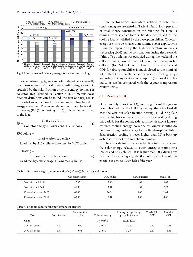
The whole building consumption for heating and cooling is presented in Fig. 12 and Table 3. They include two simulations with two different set points for cooling. 24℃

is commonly encountered in existing building while DIN 1946 regulation allows 26℃ most of the time. Energy consumption is decreased by around 23% while applying solar air-conditioning. Additionally, set point variation has a slightly lower effect on the energy use (5% to 9% decrease respectively for net and primary energy). For this location, the building heating has the greatest impact on energy consumption even when speaking about primary energy.

Fig. 11 Yearly net energy consumption for heating and cooling


251

Fig. 12 Yearly net and primary energy for heating and cooling

Other interesting figures can be introduced here. Generally the performance of a solar air-conditioning system is specified by the solar fraction or by the energy savings per collector area (defined in Section 4.4). Numerous solar fraction definitions can be found; the first one (Eq. (4)) is the global solar fraction for heating and cooling based on energy consumed. The second definition is the solar fraction for cooling (Eq. (5)) or heating (Eq (6)), it is defined according to the load.

Collector energySF

Collector energy Boiler cons. VCC cons.=

+ + (4)

SF CoolingLoad met by ABS chiller

Load met by ABS chiller Load met by VCC chiller

=

+ (5)

SF HeatingLoad met by solar storage

Load met by solar storage Load met by boiler

=

+ (6)

The performance indicators related to solar air- conditioning are presented in Table 4. Nearly forty percents of total energy consumed in the building for H&C is coming from solar collectors. Besides, nearly half of the cooling load is satisfied by the absorption chiller. Collector energy seems to be smaller than common solar applications. It can be explained by the high temperature in panels (decreasing yield) and no consumption during the weekend. If this office building was occupied during the weekend the collector energy would reach 400 kWh per square meter collector (for 24℃ set point). Finally, the yearly thermal COP for absorption chiller is much closed to the nominal value. The COPelec reveals the ratio between the cooling energy and solar auxiliary devices consumption (Section 4.7). This indicator can be compared with the vapour compression chiller COPelec.

6.2 Monthly results

On a monthly basis (Fig. 13), some significant things can be emphasized. For the building heating, there is a load all over the year but solar fraction heating is 1 during four months. No back up system is required for heating during this period. For the cooling side, each month except January requires cooling energy. Nevertheless winter months do not have enough solar energy to run the absorption chiller. Solar fraction cooling is never higher than 0.7, a back up system is involved for these eleven months.

The other definition of solar fraction informs us about the solar energy related to other energy consumptions (boiler and VCC chiller). It is higher than 80% during six months. By reducing slightly the both loads, it could be possible to achieve 100% half of the year.

Table 3 Yearly net energy consumption (kWh/(m2·year)) for heating and cooling

Gas boiler energy VCC chiller Solar auxiliaries Sum of all

Solar air-cond. 24℃ 47.33 5.68 1.81 54.83

Solar air-cond. 26℃ 46.80 3.91 1.51 52.23

Classical air-cond. 24℃ 60.46 10.98 0.00 71.44

Classical air-cond. 26℃ 60.05 8.01 0.00 68.06

Table 4 Solar air-conditioning performance indicators

Case

Solar fraction

Solar fraction cooling

Collector energy

Primary energy savings per collector area

Yearly ABS COP

Electrical COP

Units — — kWh/m2coll kWh/m2

coll — —

24℃ set point 0.43 0.47 350.19 192.12 0.70 9.85

26℃ set point 0.41 0.49 310.80 173.44 0.67 8.86


252

6.3 Daily results

Distribution of cooling energy between both chillers can be determined by a daily analysis. For days with low cooling load, the cooling load is generally satisfied by the absorption chiller only. Some days have higher cooling load. For the hotter days, the variation of the cooling load through the day is presented in Fig. 14. It is characterized by a peak value at the beginning of the cooling system operation, an increasing cooling load until 5 p.m. and a decrease to the end of the occupancy period. This kind of curve is systematically encountered from May to September. For

slightly hot day, the cooling load from 7 a.m. to 4–6 p.m. is handled by the absorption chiller. The early morning peak implies a higher minimal temperature for absorption chiller while the end of the day is less sunny; it leads to the start of VCC chiller.

For a really hot day such as the 9th of July (Fig. 14), both chillers have an alternate operation. Temperature at the top of the water storage “TfeedABS” varies with the contribution of the collector field and the water drawing of the absorption chiller. As soon as the storage temperature is higher than the threshold “TminABS+3” (see Section 4.1), the absorption chiller starts. If the temperature is not high

Fig. 13 Monthly results

Fig. 14 Cooling power for the 9th July (very hot day)


253

enough to operate the absorption chiller, it stops. There are potentially between 10 and 20 switches between both chillers during one day.

The room temperature is not displayed but matches the set point (24℃ 0.5℃) every time.

6.4 Building auxiliaries consumption

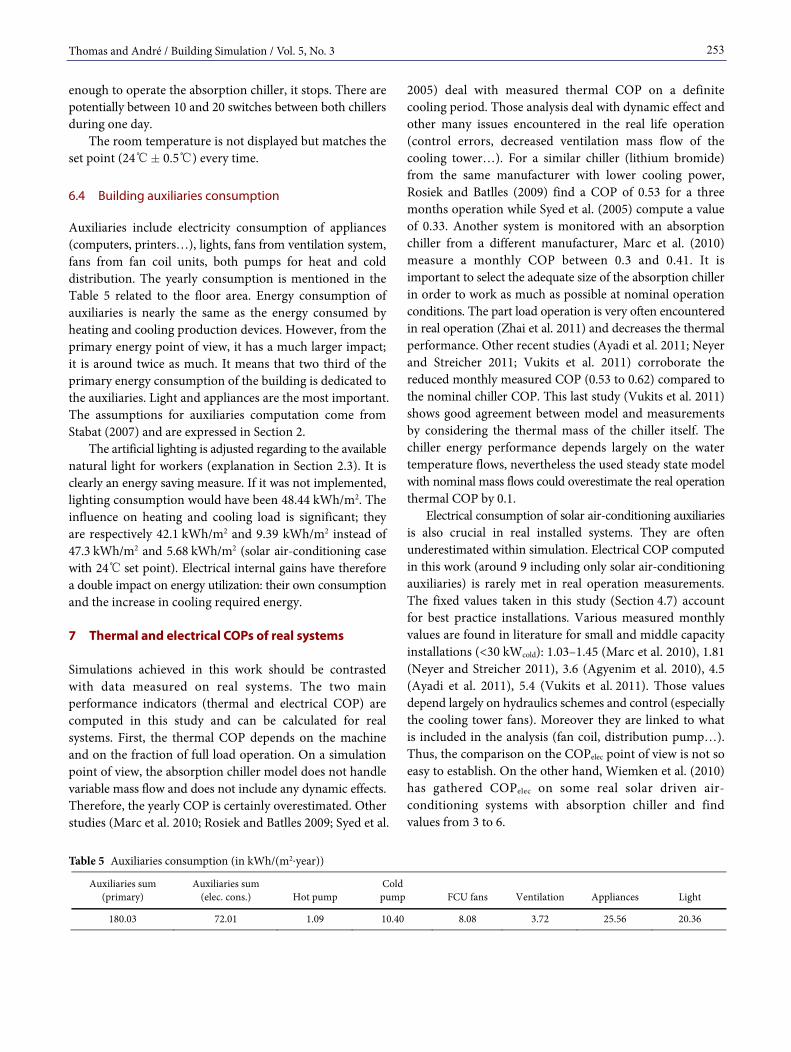
Auxiliaries include electricity consumption of appliances (computers, printers…), lights, fans from ventilation system, fans from fan coil units, both pumps for heat and cold distribution. The yearly consumption is mentioned in the Table 5 related to the floor area. Energy consumption of auxiliaries is nearly the same as the energy consumed by heating and cooling production devices. However, from the primary energy point of view, it has a much larger impact; it is around twice as much. It means that two third of the primary energy consumption of the building is dedicated to the auxiliaries. Light and appliances are the most important. The assumptions for auxiliaries computation come from Stabat (2007) and are expressed in Section 2.

The artificial lighting is adjusted regarding to the available natural light for workers (explanation in Section 2.3). It is clearly an energy saving measure. If it was not implemented, lighting consumption would have been 48.44 kWh/m2. The influence on heating and cooling load is significant; they are respectively 42.1 kWh/m2 and 9.39 kWh/m2 instead of 47.3 kWh/m2 and 5.68 kWh/m2 (solar air-conditioning case with 24℃ set point). Electrical internal gains have therefore a double impact on energy utilization: their own consumption and the increase in cooling required energy.

7 Thermal and electrical COPs of real systems

Simulations achieved in this work should be contrasted with data measured on real systems. The two main performance indicators (thermal and electrical COP) are computed in this study and can be calculated for real systems. First, the thermal COP depends on the machine and on the fraction of full load operation. On a simulation point of view, the absorption chiller model does not handle variable mass flow and does not include any dynamic effects. Therefore, the yearly COP is certainly overestimated. Other studies (Marc et al. 2010; Rosiek and Batlles 2009; Syed et al.

2005) deal with measured thermal COP on a definite cooling period. Those analysis deal with dynamic effect and other many issues encountered in the real life operation (control errors, decreased ventilation mass flow of the cooling tower…). For a similar chiller (lithium bromide) from the same manufacturer with lower cooling power, Rosiek and Batlles (2009) find a COP of 0.53 for a three months operation while Syed et al. (2005) compute a value of 0.33. Another system is monitored with an absorption chiller from a different manufacturer, Marc et al. (2010) measure a monthly COP between 0.3 and 0.41. It is important to select the adequate size of the absorption chiller in order to work as much as possible at nominal operation conditions. The part load operation is very often encountered in real operation (Zhai et al. 2011) and decreases the thermal performance. Other recent studies (Ayadi et al. 2011; Neyer and Streicher 2011; Vukits et al. 2011) corroborate the reduced monthly measured COP (0.53 to 0.62) compared to the nominal chiller COP. This last study (Vukits et al. 2011) shows good agreement between model and measurements by considering the thermal mass of the chiller itself. The chiller energy performance depends largely on the water temperature flows, nevertheless the used steady state model with nominal mass flows could overestimate the real operation thermal COP by 0.1.

Electrical consumption of solar air-conditioning auxiliaries is also crucial in real installed systems. They are often underestimated within simulation. Electrical COP computed in this work (around 9 including only solar air-conditioning auxiliaries) is rarely met in real operation measurements. The fixed values taken in this study (Section 4.7) account for best practice installations. Various measured monthly values are found in literature for small and middle capacity installations (<30 kWcold): 1.03–1.45 (Marc et al. 2010), 1.81 (Neyer and Streicher 2011), 3.6 (Agyenim et al. 2010), 4.5 (Ayadi et al. 2011), 5.4 (Vukits et al. 2011). Those values depend largely on hydraulics schemes and control (especially the cooling tower fans). Moreover they are linked to what is included in the analysis (fan coil, distribution pump…). Thus, the comparison on the COPelec point of view is not so easy to establish. On the other hand, Wiemken et al. (2010) has gathered COPelec on some real solar driven air- conditioning systems with absorption chiller and find values from 3 to 6.

Table 5 Auxiliaries consumption (in kWh/(m2·year))

Auxiliaries sum (primary)

Auxiliaries sum (elec. cons.)

Hot pump

Cold pump

FCU fans

Ventilation

Appliances

Light

180.03 72.01 1.09 10.40 8.08 3.72 25.56 20.36


254

8 Conclusion and prospects

A comprehensive coupling between an office building and a solar air-conditioning application was presented, and provided results about the whole energy consumption. A typical European office building was defined closely to the real life operation. As modelling hypothesis influence very much the energy consumption, all the parameters and the characteristics of the model are described. Moreover, almost all air-conditioning devices have their parameters taken in manufacturer’s data sheets.

The simulation includes many models, the structure becomes easier understandable by dividing the problem into three parts: building; emission & distribution; production & storage. It is also done in this way in the TRNSYS environment. Its modularity gives the possibility to optimize or replace some parts in further work.

The comparison between classical and solar air- conditioning was achieved for two cooling set points. The first one is commonly observable in buildings while the second one is coming from a standard. Classical air-conditioning has a total net energy consumption of around 70 kWh/(m2·year) while solar air-conditioning falls to the order of magnitude of 50 kWh/(m2·year). A decrease of 22% is thus encountered. It is a considerable decrease in energy consumption according to the heat and cold production but a lighter effect on the total building energy consumption. Besides, the higher cooling set point shrinks the energy consumption by around 5%. On the energy point of view, the solar air-conditioning is more interesting when the building is moderately cooled down.

The solar collector size was set according to the roof size. It is a crucial parameter of the solar air-conditioning system. Energy savings are directly linked to its value; it is then possible to save much more energy by installing an enormous solar collector field. If there is neither space nor economical limit, the solar auxiliaries would be an important part of the energy balance. The COPelec is then an excellent indicator for solar system energy performance.

The auxiliaries consumption are also computed considering a common building use. One of the key facts is that auxiliaries consumption in terms of primary energy is always really higher than energy used for heating and cooling. As shown for lighting, their use adds electricity consumption and increases cooling load in the room. Reducing the building auxiliaries consumption by using energy efficient electrical devices seems to be very interesting.

This work reveals also some limitations of the current simulation environment. As explained below, the thermal model of absorption chiller does not handle variable mass flow and does not include any dynamic effects. Compared to the mean measured values on a long period, the COP is

probably overestimated by at least 0.1. The low COP values measured can be due to a non optimal design of the system and control. Moreover, the real operation has to deal with system failures and other control malfunctions that are not implemented into simulation environment.

The evaluation of electricity consumption of solar air- conditioning auxiliaries has been roughly achieved. Compared to the real operation, the simulated electrical COP is quite high. As for the thermal COP, some of the real life issues cannot be implemented into the simulation. Despite of this, the simulation environment should implement precise pipe network, pump and fan models to have a more accurate electricity consumption evaluation. The electrical COP is the main challenge of the current real solar air-conditioning systems.

Finally, the latent load is handled in a very simple way, independently of fan coil operation. It should be added to the fan coil unit model to couple sensible and latent loads.

The simulation environment is a comprehensive building and systems model, it allows evaluating the potential energy savings of various design options by modifying some parameters or by implementing new control strategies for lighting, ventilation, solar protections, heating, cooling…

References

AEC (2007). Heat & Cool FG cooling tower. http://www.aecinternet.com/ images_products/files/FG%20Cooling%20Tower%20LO.pdf. Accessed 13 Jul. 2011.

Agyenim F, Knight I, Rhodes M (2010). Design and experimental testing of the performance of an outdoor LiBr/H2O solar thermal absorption cooling system with a cold store. Solar Energy, 84: 735 744.

Alessandrini JM, Fleury E, Filfi S, Marchio D (2006). Impact de la gestion de l’éclairage et des protections solaires sur la consommation d’énergie de bâtiments de bureaux climatisés. In: Proceedings of Climamed, 3ème congrès méditerranéen des climaticiens, Lyon, France. (in French)

Ayadi O, Mauro A, Motta M (2011). Solar heating and cooling system for office building in italy; description and performance assessment. In: Proceedings of the 4th Ostbayerisches Technologie-Transfer- Institut Solar Air-Conditioning Conference 2011, Larnaca, Cyprus.

Barbosa RM, Mendes N (2008). Combined simulation of central HVAC systems with a whole-building hygrothermal model. Energy and Buildings, 40: 276 288.

Bujedo L, Rodriguez J, Martícnez PJ, Rodríguez LR, Vicente J (2008). Comparing different control strategies and configurations for solar cooling. In: Proceedings of the International Solar Energy Society Eurosun 2008 Conference, Lisboa, Portugal.

CARRIER (2007). Fan Coil Unit Carrier 42N documentation, http://www.ahicarrier.com/pdf/PD/42N_PD.pdf. Accessed 13 Jul. 2011.


255

Casals XG (2006). Solar absorption cooling in Spain: Perspectives and outcomes from the simulation of recent installations. Renewable energy, 31: 1371 1389

Eicker U, Pietruschka D (2009). Design and performance of solar powered absorption cooling systems in office buildings. Energy and Buildings, 41: 81 91.

Henning H-M (2007). Solar-Assisted Air-Conditioning in Buildings: A Handbook for Planners, 2nd edn. Vienna: Springer-Verlag/Wien.

Henning H-M (2008). Solar Cooling components and systems—An overview. Solar Air-Conditioning International Seminar, 2009, Munich, Germany.

Herold KE, Radermacher R, Klein SA (1996). Absorption Chillers and Heat Pumps. Boca Raton, USA: CRC Press.

Jakob U (2011). Overview market development and potential for solar cooling with focus on the Mediterranean area. In: Proceedings of the 5th European Solar Thermal Energy Conference (ESTEC 2011) (pp. 59 64), Marseille, France.

Kagerer F, Herkel S (2010). Concepts for Net Zero Energy Buildings in refurbishment projects. In: Proceedings of the International Solar Energy Society Eurosun 2010 Conference, Graz, Austria.

Klein SA (2007). TRNSYS 16 Program Manual. SEL, University of Wisconsin, Madison, USA.

Marc O, Lucas F, Sinama F, Monceyron E (2010). Experimental investigation of a solar cooling absorption system operating without any backup system under tropical climate. Energy and Buildings, 42: 774 782.

MATLAB (2007). The Mathworks Inc., http://www.mathworks.com, Natick, USA.

Mugnier D (2002). Rafraîchissement solaire de locaux par sorption: optimisation théorique et pratique. PhD Dissertation, Ecole des mines de Paris, France. (in French)

Neyer D, Streicher W (2011). Monitoring and simulation results of two small scale solar cooling plants. In: Proceedings of the 4th Ostbayerisches Technologie-Transfer-Institut Solar Air-Conditioning Conference 2011, Larnaca, Cyprus.

Ortiz M, Barsun H, He H, Vorobieff P, Mammoli A (2009). Modeling of a solar-assisted HVAC system with thermal storage. Energy and Buildings, 42: 500 509.

Rosiek S, Batlles FJ (2009). Integration of the solar thermal energy in the construction: Analysis of the solar-assisted air-conditioning system installed in CIESOL building. Renewable Energy, 34: 1423 1431.

SCHOTT ETC 16 (2003). SCHOTT Evacuated Tube Collector ETC16 http://www.schott.com/uk/english/download/solar_thermal_rd319 .pdf. Acessed 13 Jul. 2011.

Sparber W, Napolitano A (2009). IEA-SHC Task 38. List of existing solar heating and cooling installations. Available online

http://iea-shc-task38.org/documents/monitoring2. Accessed 13 Jul. 2011.

Stabat P (2007). IEA48—Description of Type 1c air-conditioned office buildings for simulation test, IEA-ECBCS Annex 48 working document.

Syed A, Izquierdo M, Rodriguez P, Maidment G, Missenden J, Lecuona A, Tozer R (2005) A novel experimental investigation of a solar cooling system in Madrid. International Journal of Refrigeration, 28: 859 871.

Thomas S, André P (2009a). Dynamic simulation of a complete solar assisted air-conditioning system in an office building using TRNSYS. In: Proceedings of the 11th International Building Performance Simulation Association Conference (BS2009), Glasgow, UK.

Thomas S, André P (2009b). Control strategies study of a complete solar assisted air conditioning system in an office building using TRNSYS. In: Proceedings of the 3rd Ostbayerisches Technologie- Transfer-Institut Solar Air-Conditioning Conference 2009, Palermo, Italy.

Thür A (2010). Monitoring program of small-scale solar heating and cooling systems within IEA-SHC Task 38 – Procedure and first results. In: Proceedings of the International Solar Energy Society Eurosun 2010 Conference, Graz, Austria.

TRNSYS (2006). TRNSYS Simulation Studio, Version 16.00.0038 Licensed to University of Liège.

Vukits M, Altenburger F, Thür A (2011). Operation and energy performance as well as simulation results of two solar cooling plants in Gleisdorf. In: Proceedings of the 4th Ostbayerisches Technologie-Transfer-Institut Solar Air-Conditioning Conference 2011, Larnaca, Cyprus.

WESPER VLH HE 804 (2005). Air-to-Water Reverse Cycle Heat Pumps VLH 504 to 1204 Technical Brochure, Wesper S.A.S., Pons, France.

Wiemken E, Wewior JW, Elias AP, Nienborg B, Koch L (2010). Performance and perspectives of solar cooling. In: Proceedings of the International Solar Energy Society Eurosun 2010 Conference, Graz, Austria.

YAZAKI (2008). Water Fired Chiller/Chiller-Heater WFC-S Series documentation http://www.yazakienergy.com/waterfiredperformance.htm. Accessed 13 Jul. 2011.

Zhai XQ, Qu M, Li Y, Wang RZ (2011). A review for research and new design options of solar absorption cooling systems. Renewable and Sustainable Energy Reviews, 15: 4416 4423.

Zweifel G, Dorer V, Koschenz M, Weber A (1995). Building energy and system simulation programs: model development, coupling and integration. In: Proceedings of 9th International Building Performance Simulation Association Conference (BS2005), Madison, Wisconsin, USA.

Numerical simulation and performance assessment of an absorption solar air-conditioning system...

Documents

Transcript of Numerical simulation and performance assessment of an absorption solar air-conditioning system...