Numerical Simulatio onf Supersonic Plume in a Cowl...

©Freund Publishing House Ltd. London International Journal of Turbo and Jet Engines, 16, 241-253(1999)

Numer ica l S imula t ion of Superson ic P l u m e in a C o w l - P l u g Nozz le C o n f i g u r a t i o n }

Tony W. H. Sheu

Department of Naval Architecture and Ocean Engineering, National Taiwan University, 73 Chou-Shan Rd., Taipei, Taiwan, R.O.C.

Abstract

We present in this paper a method of characteristics which permits the investigation of supersonic inviscid fluid flow in an axisymmetric cowl plug nozzle. The characteristic analysis involves use of a space marching solution algorithm. For computation of the steady-state solution of hyperbolic equations, the inlet condition is one key to success in providing a good representation of the physics of the flow. To achieve this goal, we apply the asymptotic and perturbation method to determine the supersonic startline M= 1.04 by expanding flow variables and thermodynamic properties with respect to values computed under the transonic condition M=l. An inherent feature of the method of characteristics is its ability to solve for flows in the characteristic network along which left- and right-running characteristic equations apply. Along these characteristic lines, dependent variables are solved for from their respective compatibility equations. A modified Euler predictor-corrector two-step numerical scheme is used to discretize characteristic and compatibility equations. The analysis proceeds with solving the supersonic flow through the plug nozzle, for which the physical domain is bounded by the free pressure boundary that is not determined a priori. In this study, different ambient pressures are considered to investigate their effects on the gas dynamics in the flow passage. Results are presented in terms of pressure, temperature, and Mach number distributions. Obtained also from this study is a clear understanding of the effect of pressure ratios on the shape of the plume.

Nomenclature

α Mach angle

δ free parameter in (1)

γ ratio of specific heats

ρ density

θ f low angle

a sound speed

a0 stagnation sound speed

g gravitational constant

Μ Mach number

ρ pressure

R gas constant

r spatial independent variable along the

r-direction

Τ temperature

w,ν velocity components in the x,r directions,

respectively

X spatial independent variable along the

x-direction

Introduction

In the last three decades, different areas

regarding simulation of high speed aerodynamics

have witnessed t remendous developments , examples

of which are grid generation techniques, solution

algori thms and computer hardware capabilities. All

these developments have led to the stage where it is

nowadays possible to consider the f low simulation

as a tool for use in complex aerodynamic f low

analysis. This is particularly the case when

experimental databases are scarce or incomplete. In

this light, numerical analysis of an aerodynamic

f low field in a single plug nozzle fo rmed the core of

the present study. It was best hoped that much

physical insight could be obtained cost-effect ively

through the f low simulation technique.

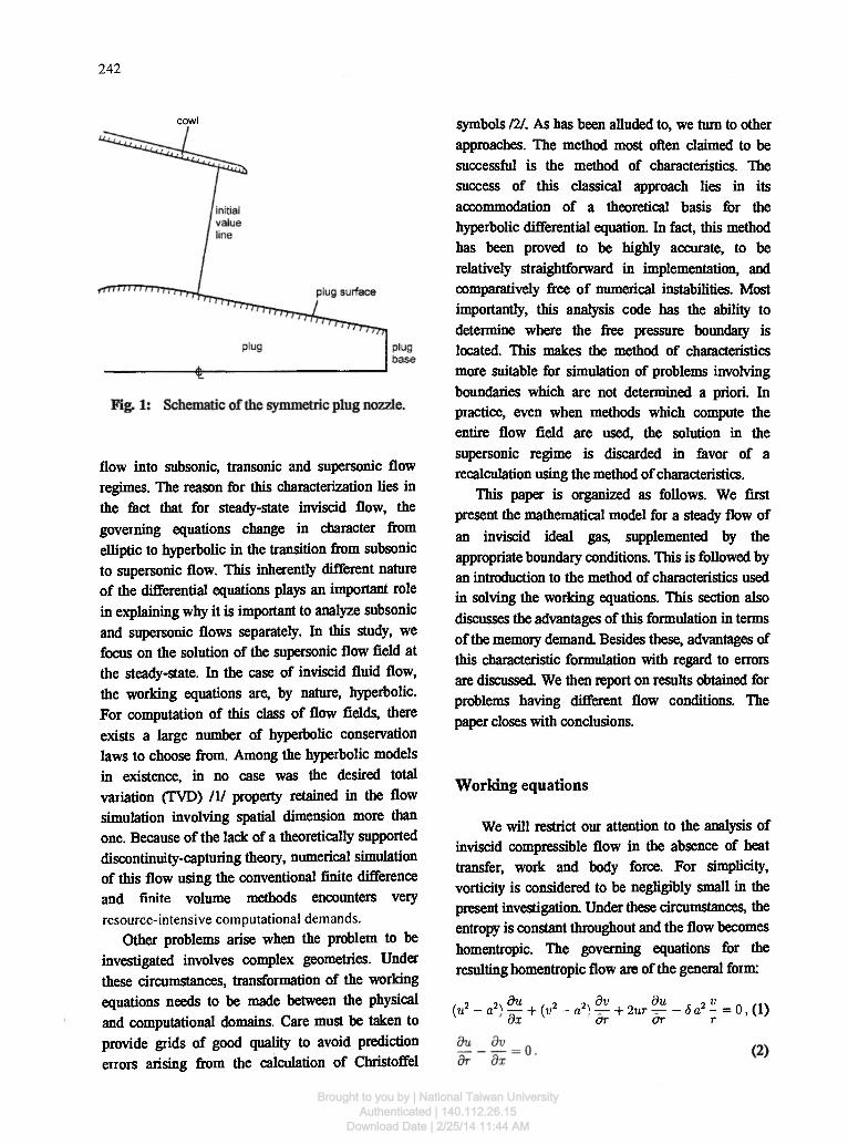
We consider in this paper inviscid f low in a

single plug nozzle, shown schematical ly in Fig. 1. It

is customary to characterize the propulsive nozzle

241 Brought to you by | National Taiwan UniversityAuthenticated | 140.112.26.15

Download Date | 2/25/14 11:44 AM

242

cowl

flow into subsonic, transonic and supersonic flow regimes. The reason for this characterization lies in the fact that for steady-state inviscid flow, the governing equations change in character from elliptic to hyperbolic in the transition from subsonic to supersonic flow. This inherently different nature of the differential equations plays an important role in explaining why it is important to analyze subsonic and supersonic flows separately. In this study, we focus on the solution of the supersonic flow field at the steady-state. In the case of inviscid fluid flow, the working equations are, by nature, hyperbolic. For computation of this class of flow fields, there exists a large number of hyperbolic conservation laws to choose from. Among the hyperbolic models in existence, in no case was the desired total variation (TVD) I I I property retained in the flow simulation involving spatial dimension more than one. Because of the lack of a theoretically supported discontinuity-capturing theory, numerical simulation of this flow using the conventional finite difference and finite volume methods encounters very resource-intensive computational demands.

Other problems arise when the problem to be investigated involves complex geometries. Under these circumstances, transformation of the working equations needs to be made between the physical and computational domains. Care must be taken to provide grids of good quality to avoid prediction errors arising from the calculation of Christoffel

symbols 111. As has been alluded to, we turn to other approaches. The method most often claimed to be successful is the method of characteristics. The success of this classical approach lies in its accommodation of a theoretical basis for the hyperbolic differential equation. In fact, this method has been proved to be highly accurate, to be relatively straightforward in implementation, and comparatively free of numerical instabilities. Most importantly, this analysis code has the ability to determine where the free pressure boundary is located. This makes the method of characteristics more suitable for simulation of problems involving boundaries which are not determined a priori. In practice, even when methods which compute the entire flow field are used, the solution in the supersonic regime is discarded in favor of a recalculation using the method of characteristics.

This paper is organized as follows. We first present the mathematical model for a steady flow of an inviscid ideal gas, supplemented by the appropriate boundary conditions. This is followed by an introduction to the method of characteristics used in solving the working equations. This section also discusses the advantages of this formulation in terms of the memory demand Besides these, advantages of this characteristic formulation with regard to errors are discussed We then report on results obtained for problems having different flow conditions. The paper closes with conclusions.

Working equations

We will restrict our attention to the analysis of inviscid compressible flow in the absence of heat transfer, work and body force. For simplicity, vorticity is considered to be negligibly small in the present investigation Under these circumstances, the entropy is constant throughout and the flow becomes homentropic. The governing equations for the resulting homentropic flow are of the general form;

. , o, du , ,N dv „ du t , » „ . . . (u2 - a2 — + (v2 - a2 — + 2ur — - δ a2 - = 0 , ( 1 ) d x or or r

Brought to you by | National Taiwan UniversityAuthenticated | 140.112.26.15


243

In the above, a is the sound speed, which can be

easily shown as a function o f a specific heat ratio, γ,

the stagnation sound speed, a 0 , and the velocity

magnitude:

a2 = — ~r— (u2 + v2). (3)

In equation (1), 5=0 corresponds to the planar flow and δ=1 to the axisymmetric flow. We denote by u and ν the flow velocity components in the χ and r directions, respectively. It is a simple matter to show that equation (1) is derived from the Euler equation through use of a continuity equation Equation (2) represents, in essence, the irrotationary condition. As for equation (3), it is derived as a direct result of energy conservation

Following conventional practice /3/, the above hyperbolic differential system is transformed equivalently into the following set of characteristic and compatibility equations. Along the left-running characteristic line, the working equations are obtained as follows:

^ = tan (0 + α), ax dlul δ sin θ sin a , άθ - -p-p cota + - — — — - dr — 0 . |u| r sin(0 ± a)

(4)

(5)

In the opposite direction, the working equations

along a right-running characteristic line are

represented by

dr .. . — = tan [θ - a), ax dlul δ sin θ sin a , — -dr = 0. |«| r sin(0 — a)

(6)

(7)

In equations (4 -7 ) , θ is the flow angle, α is the

Mach angle, and |u| = ( h 2 + v 2 ) " 2 is the velocity

magnitude. As with many other numerical analyses,

we assume that the gas under investigation is

regarded ideal. This implies that the following

equation o f state holds in the flow:

ρ = pRT. (8)

In the above equation, ρ is the pressure, ρ is the

density, Τ is the temperature and R is the gas

constant Before embarking on a numerical treatment of

equations given in (5-8), which are subject to a prescribed inlet condition, it is instructive to summarize here other rederived thermodynamic properties. Equations (4-7) constitute the core of the analysis, from which the primary dependent variables |w| and θ are solved. This is followed by calculation of the velocity components u and ν from |m| and Θ. With a velocity field u determined, the following thermodynamic relationships apply:

T = T0- (u2 + ,r),

P=(

27 Rg

P2 ] 1 + *ζ±λΡ>

(9)

(10)

In equation (10), Μ is the Mach number, which is computed as

M = (τ RgT) 1/2 • (11)

In the above, g denotes the gravitational constant The above derivation also involves T0 and Po, which are the stagnation temperature and pressure, respectively. Having obtained the thermodynamic properties given in equations (9-10), the density of the gas is determined from the equation of state as follows :

p = RT (12)

Determination of supersonic startline

Equations (4-7) represent characteristic and compatibility conditions along left- and right-running characteristics. They constitute the working equations for the primary variables |m| and Θ. In the characteristic network, we seek the solution of equations (4-7) subject to the appropriate boundary conditions described in the next section Starting from the initial data for |m| and Θ, working equations can be solved in the network of characteristics. In seeking to perform accurate simulation of a hyperbolic equation, specification of primary variables at the supersonic startline is a



244

major consideration provided that the working equations are to be solved using a charac-teristics-based method. Such a method applies only to the hyperbolic differential system. Therefore, the validity of applying the method of characteristics to obtain solutions requires specification of supersonic flow at the nozzle inlet

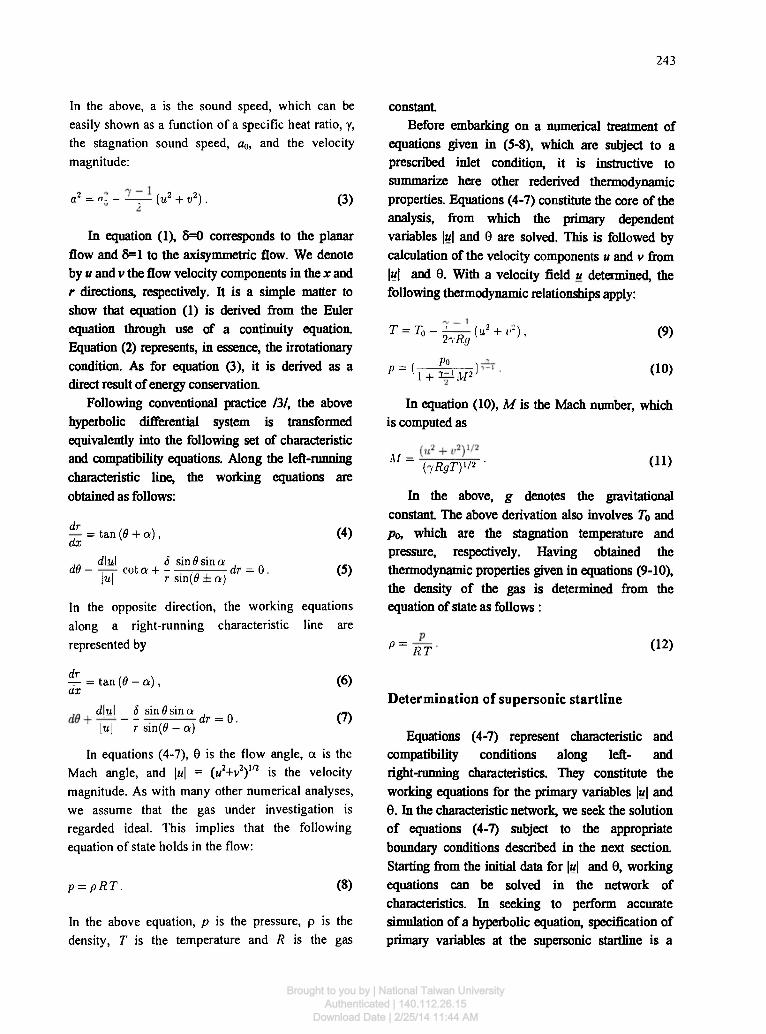
For accurate prediction of the flow physics in the nozzle, the determination of a supersonic staitline is important and provided another motivation for the present work. With the objective of determining a line of constant Mach number (M > 1) as the supersonic startline in the prediction of supersonic nozzle flow, we follow the same approach as that given in /4/. According to Thompson and Flack 151, we can apply the asymptotic and perturbed method to represent flow variables at Μ = 1.04 in terms of those at Mach number M = 1 and small perturbation quantities. The resulting supersonic startline for Μ = 1.04 is shown schematically in Fig. 2. A detailed exposition of the numerical method leading to this supersonic startline has been given in 161 along with a brief introduction to the asymptotic and perturbation method.

Fig. 2: The supersonic startline for the Mach number with the value of 1.04.

Numerical model

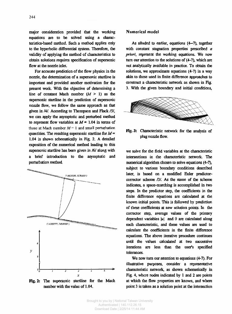
As alluded to earlier, equations (4—7), together with constant stagnation properties prescribed a priori, represent the working equations. We now turn our attention to the solutions of (4-7), which are not analytically available in practice. To obtain the solutions, we approximate equations (4-7) in a way akin to those used in finite difference approaches to construct a characteristic network as shown in Fig. 3. With the given boundary and initial conditions,

Fig. 3: Characteristic network for the analysis of plug nozzle flow.

we solve for the field variables at the characteristic intersections in the characteristic network. The numerical algorithm chosen to solve equations (4-7), subject to various boundary conditions described later, is based on a modified Euler predictor-corrector scheme /3Λ As the name of the scheme indicates, a space-marching is accomplished in two steps. In the predictor step, the coefficients in the finite difference equations are calculated at the known initial points. This is followed by prediction of these coefficients at new solution points. In the corrector step, average values of the primary dependent variables |M| and θ are calculated along each characteristic, and these values are used to calculate the coefficients in the finite difference equations. The above iterative procedure continues until the values calculated at two successive iterations are less than the user's specified tolerances.

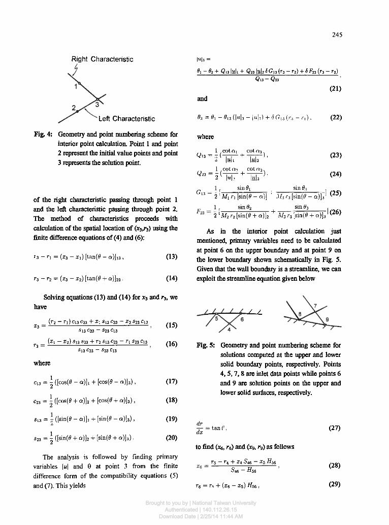
We now turn our attention to equations (4-7). For illustrative purposes, consider a representative characteristic network, as shown schematically in Fig. 4, where nodes indicated by 1 and 2 are points at which the flow properties are known, and where point 3 is taken as a solution point at the intersection



245

Right Characteristic l«|.i =

Left Characteristic

Fig. 4: Geometry and point numbering scheme for interior point calculation. Point 1 and point 2 represent the initial value points and point 3 represents the solution point.

of the right characteristic passing through point 1 and the left characteristic passing through point 2. The method of characteristics proceeds with calculation of the spatial location of (x3,r3) using the finite difference equations of (4) and (6):

73 - η = (x3 - x,) [tan(0 - α)]ΐ3 ,

Ti-T 2 = (x3 - Xi) [tan(0 + a)]23 ·

(13)

(14)

Solving equations (13) and (14) for x3 and r3, we have

x3

r3 =

where

(r2 - n ) Ci3 c23 + Xi s13 c23 - x2 «23 C13 «13 C23 - S23 C13

(xi - x2) S13 523 + r2 Sis c23 - η S23 C13 «13 C23 - «23 Cl3

C13 = \ ([cos(0 - α)]ι + [cos(0 - α)]3),

C23 = \ ([cos(0 + α)]2 + [cos(0+ α)]3),

s13 = - ([sin(0 - α)]ι + [sin{(9 - α)]3),

s23 = \ ([sin(0 + α)]2 + [sin(0 + α)]3) ·

(15)

(16)

(17)

(18)

(19)

(20)

The analysis is followed by finding primary

variables |«| and θ at point 3 from the finite

difference form of the compatibility equations (5)

and (7). This yields

01 - 02 + Q13 lull + Q23 |a|2 <5 G13 (r3 - r2) + δ F23 (r3 - r2) Ql3 - Q23

and

03 = 01 - 013 (|«|3 - M l ) + δ GM ('·.·! - Γ|) .

where

1 cot «ι coto:3 Q13 = Χ (-ΓΊ ·" ~T~i—) ·

l«li Iii|3 1 cot (Xi cot.«3.

Q-23 = Τ (-j—j 1- -7-j ) · 2 |«|> Im|3

sin 0i sin 0:!

G l 3 2 lMx rι [sin(0 - a)] ' M3 r3 [sin(0 - a)]3

sin 02 + sin U3

2 L M2 r2 [sin(0 + a)]2 M3 r3 [sin(0 + a)]3

(21)

(22)

(23)

(24)

(25)

1(26)

As in the interior point calculation just mentioned, primary variables need to be calculated at point 6 on the upper boundary and at point 9 on the lower boundary shown schematically in Fig. 5. Given that the wall boundary is a streamline, we can exploit the streamline equation given below

J /

Fig. 5: Geometry and point numbering scheme for solutions computed at the upper and lower solid boundary points, respectively. Points 4 , 5 , 7 , 8 are inlet data points while points 6 and 9 are solution points on the upper and lower solid surfaces, respectively.

dr dx

= tan f

to find (xe, r6) and (x9, r9) as follows

_ rb - r4 + x4 ^46 ~ xi HS6

S46 - #56

re = + (x6 ~ X5) #56 ,

(27)

(28)

(29)



246

Xg = • r T + x7 S79 - x& Hs<

S79 — Η89

rg = r8 + (19 - ^s) #S9 ,

where

#56 = - (tan 05 + tan 06)

#89 = 2 (tan + tan09),

•S46 = 2 ( t a n (^4 + 04) + tan(ö6 + α6)),

5T9 = - (tan(07 - a9) + tan(ft, - a9)).

(30)

(31)

(32)

(33)

(34)

(35)

Having determined where the solution points are located, we now compute the remaining primary variables |w| at points 6 and 9. These values can be calculated as follows from the appropriate compatibility equations:

Ne = \ m +

Iii 9 = Ii 7 •

ö 6 - ö l + dG46 (rß-r . , )

-(θ*

Θλ6

9 r ) + δ G-g (r9 - r - )

where

sin »4 + • sin t 2 M47-4 sin(04 + q4) A/6 r6 sin(06 + q6)

C79 = ö ( sin 07 sin dg

(36)

(37)

r)<38)

)(39) 2 M7 r7 sin(07 - Q-) Mg r9 sin(09 - a9)

The other primary variables θ at boundary points

are obtained as

dv

θ6 = tan_1(—)δ6 ,

cLv Qg = tan_1(—)89 .

(40)

(41)

To conclude the present analysis, we turn to determination of the plume configuration. In Fig. 6, we designate points 10, 11, 13, and 14 as initial data points at which flow properties are known. Points 12 and 15 are solution points at the intersection of the characteristics passing through points 10 and 13 and at the streamlines passing through points 11 and 14. The properties at points 12 and 15 are, by definition, known, which implies t h a t pw = p \ 2 a n d p X A = p\5. As

Free Pressure Boundary 1 2 ,

Free Pressure Boundary

Fig. 6: Geometry and point numbering scheme for solutions computed on the upper and lower pressure boundary points respectively. Points 10, 11, 13, 14 denote the initial data points, while points 12 and 15 are solution points at the upper and lower free pressure boundaries, respectively.

before, the spatial coordinates (χι* Λ2) and (*ι5, ri5) can be determined from the characteristic equations along lines passing through points 10 and 13. The resulting coordinates at the free pressure boundary are obtained as

X12 ': - no + Zio S11 • 111 Η 1112 S1012 — #1112

Γ12 = Γιι + #1U2 (.Cl2 ~ 111) ,

^ _ Γ).| — Γ13 + X|3 Si;n3 — .C|.| #[415 Sl315 — #1115

r15 = r14 + #1115 (̂ 15 — l u ) 1

(42)

(43)

(44)

(45)

where #1112, #1415, Si 012 and S13i5 take forms similar to those shown in equations (32)-{35). At solution points 12 and 15, primary variables |w| are calculated from the equations given in (11)-(14). The results are expressed as:

|li| 12 = -̂ 13 &13 .

and

|u| 15 = MlS «15 ,

where Μ, αϊ (=13,15) are as follows :

POs M , = [(

ai = (-yRg

- i ) 7 - l J

11/2

fj> \ 1/2 1 + '

(46)

(47)

(48)

(49)



247

As to primaiy variables θ at points (*i2, Λ 2) and (*i5> r\s)> they are obtained from the respective compatibility equations, yielding

012 = 010 + [(I«|l2 - Nio) 01012 ~ <5 (̂ "-12 ~ Πο) G1012] ,

(50)

015 = 013 ^ [(|w|l5 - Ν13) 01315 ~ <5 (̂ 15 ~ Hs) G1315] ·

(51)

In the above equations, Θ10ΐ2, θ13ι5, Gi0i2 and Gi 315 are expressed as follows :

1 .cot Q10 cot Q12 . "1012 — ή l"T~i '—Π >> 2 ImIio MI2

1 COtQi3 COtOi5. "1315 — - 1 —j—;—ι—π—). 2 |u|l3 |u|l5

1 ^ sinöio ^ sin 0i2

(52)

(53)

2 Μ ίο τ ίο (sin(0 - α))10 Mn ru (sin(0 - a))12

(54)

G(315 —

i ( sin (λ·. + sinfi; 2 A/ l 3r1 3(sin(ö-«))i3 Mir, rl5 (sin(0 - «))1 5

(55)

Results and Discussion

Problem description

Of three basic types of exhaust nozzles, we consider in this study a plug nozzle through which passes the inviscid flow of a compressible ideal gas. The plug and cowl configurations are shown schematically in Fig. 1. The flow properties and spatial locations of the supersonic streamline have been specified based on the asymptotic and perturbation method. The Mach number is constant across the initial value line. The results presented here are for an ideal gas with the specific heat ratio γ = 1.337. The stagnation temperature and pressure shown in equations (9-10) take fixed values of 1750°/? and 15 psia, respectively. Under the specified stagnation conditions, thermodynamic

properties and primaiy variables at the supersonic inlet, the Mach number has a value of 1.04. Starting with the initial data, characteristic and compatibility equations can be solved in a characteristic network which extends outwards from the supersonic startline. Under these circumstances, the flow downstream of the supersonic inlet depends solely on the ambient pressure. In this study, we consider five different pressure ratios, PR ξ p o / p ^ = 4, 5, 6, 8, 9, the ratio between the ambient pressure, / w » and the stagnation pressure po.

Effect of pressure ratios on the gas dynamics

In seeking to study the effect of pressure ratios on the gas dynamics in the symmetric exhaust plug nozzle, all the simulations will be discussed on the basis of plots representing the distributions of pressure, temperature and Mach number in the flow interior bounded by the plume and the plug nozzle. In addition, the pressure distribution along the wall of the plug nozzle is also presented for purposes of illustration. We present here first the results for the case with ρο/ραώ = 4. Figure 7 shows the pressure distributions at three selected streamwise locations. The plume configuration at which the pressure takes on the value of 3.75 psia is also plotted. Revealed by this figure is that the upstream pressure takes a larger value in the vicinity of the plug nozzle wall region than in the vicinity of the plume edge. As the flow proceeds downstream to x= 10 inch, the trend is reversed.

Since the ideal gas assumption is made in the

ν (inch)

15

10 cowl

Plume

Wall m

Pressure ρ (Psia)

10 1415 20 25 30 > x (inch)

Fig. 7: Pressure distributions at planes χ = 5 in, 10 in, and 15 in for the case with PR = 4.



248

y(inch)

Plume

1200 1300 Τ Wall

1000 1100 Τ 1100 1200

Temperature T("R)

5 iS 3 20 25 S->-i(inCh)

Fig. 8: Temperature distributions at planes χ = 5 in, 10 in, and 15 in for the case with PR = 4.

ν (inch) 15

Cowl Plume

1 2 . , Μ 123 Μ Wall 1 2 3Mach Number Μ

ίο 15 20 25 30 x (inch)

Fig. 9: Mach number distributions at planes χ = 5 in, 10 in, and 15 in for the case with PR = 4.

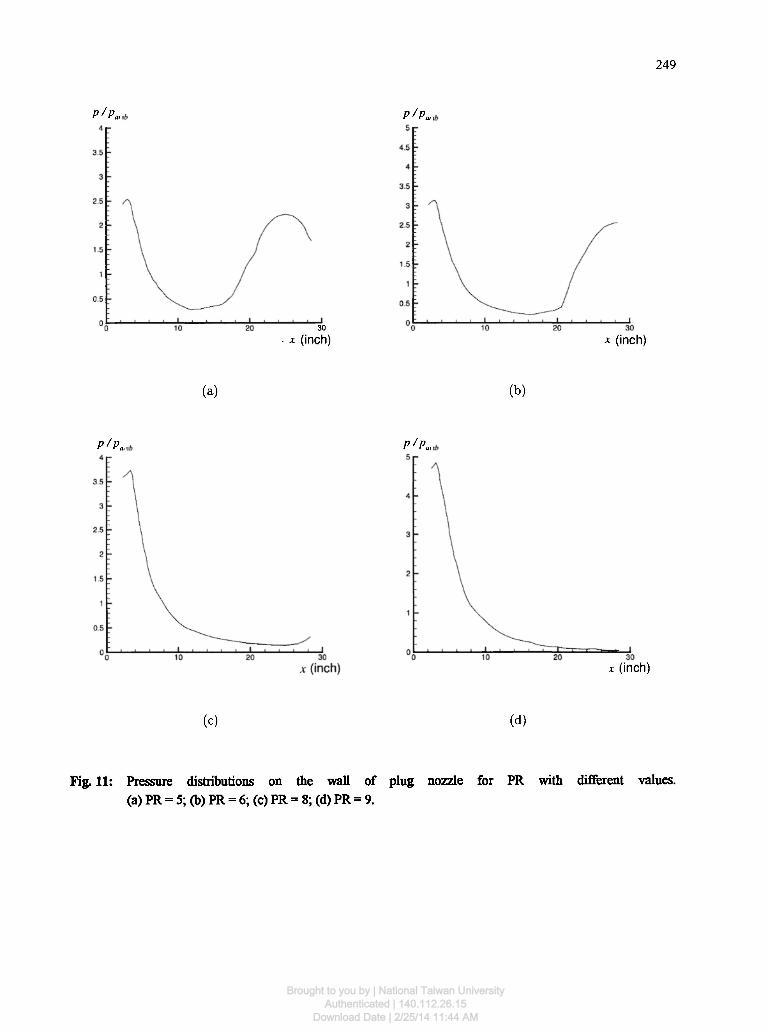
analysis, it is no surprise to find that the temperature shown in Fig. 8 has profiles similar to those plotted in Fig. 7 for the pressure. The Mach number distribution is presented in Fig. 9, which clearly reveals that the flow gradually becomes a constant Mach number in its approach to the downstream region. To close the presentation Of results for the case of PR = 4, we present in Fig. 10 the pressure distribution along the wall of the plug nozzle. The wall pressure drops sharply from the pressure computed on the upstream side. This is followed by a nearly constant pressure in the range of 8 inch ^ χ £ 13 inch. The wall pressure then increases. Due to space limitation, we do not plot the pressure or Mach number distributions for the remaining cases of PR = 5, 6, 8, 9. In Fig. 11, we plot wall pressures along the plug nozzle for other four investigated values of PR= 5,6, 8, 9. This figure provides readers with information about the effect of PR on the aerodynamic loading added to the plug nozzle.

We also plot in Fig. 12 the shapes of the plume

Po'Pamt, 5 r

1 L l t r . 1 . 1 . 5 10 15 20 25 30

X (inch)

Fig. 10: Pressure distribution along the wall of plug nozzle for the case with PR = 4.

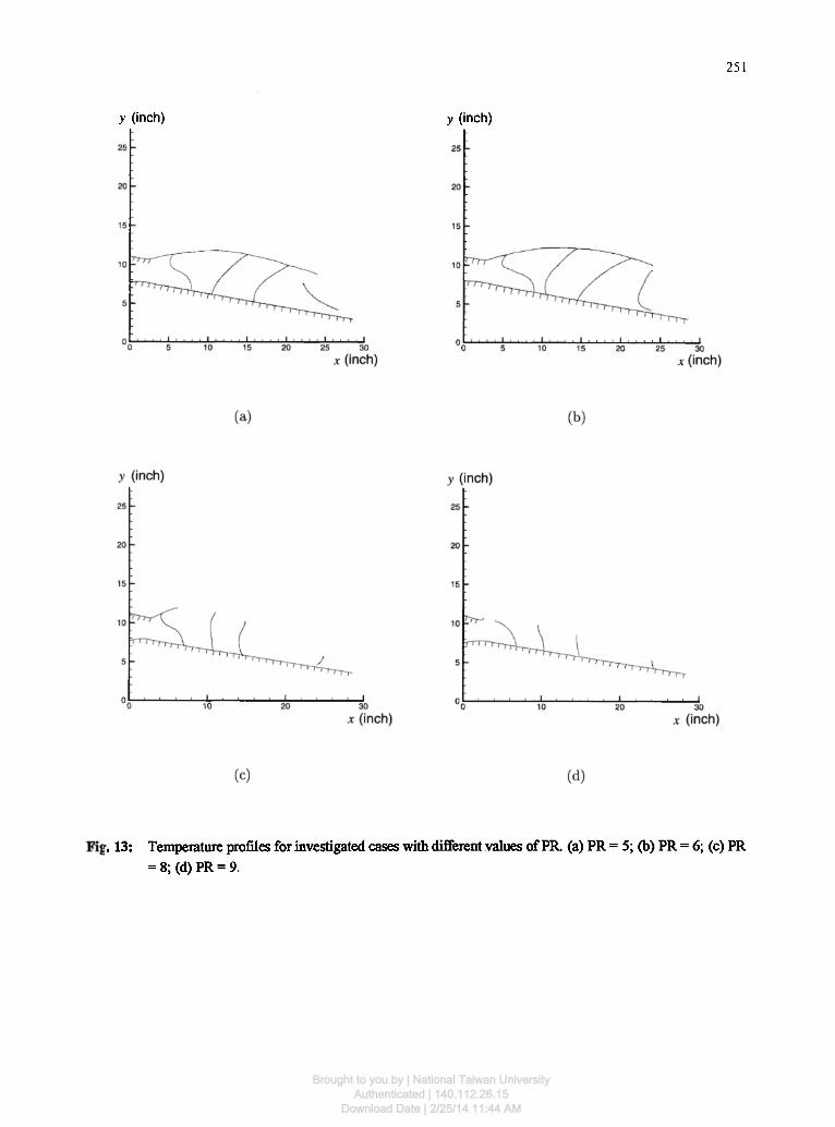
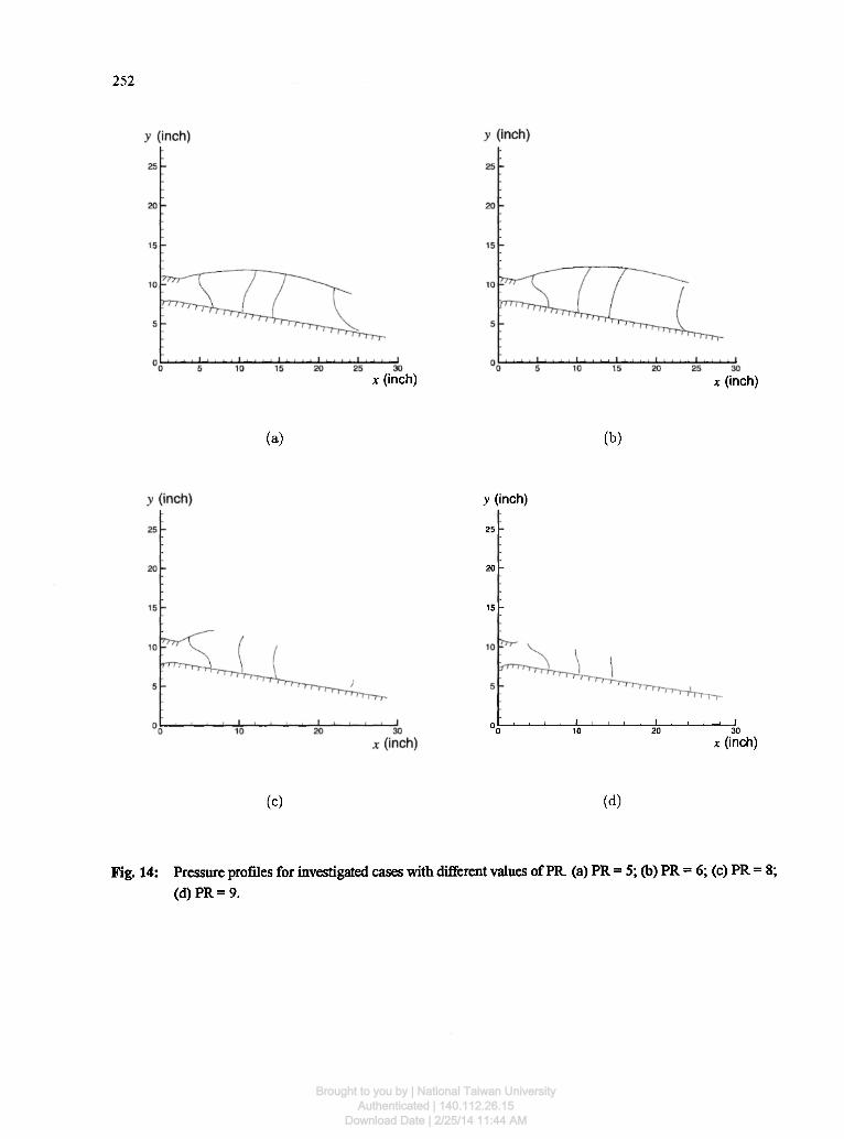
for all the investigated conditions. These figures are fundamentally useful in identifying the type of aircraft since each one has its own plume shape. We close the paper with Fig. 13, which plots the temperature profiles, and Fig. 14, which plots the pressure profiles, in the characteristic network. These plots are important for providing us with valuable knowledge for designing cooling supply slot, from which the cold film discharges into the environment

Concluding Remarks

We consider the method of characteristics a computationally efficient hyperbolic flow simulation technique to analyze problems involving an axisymmetric exhaust plug nozzle and cowl boundary. The method used to simulate this problem was chosen mainly because of the involvement of a free pressure boundary condition. Unlike con-ventional finite-difference methods, we seek solutions in a characteristic network which extends towards the downstream flow regime. The solution procedure used to construct the characteristic network utilizes the left- and right-running characteristics to determine the solution points. Along these characteristics, primary variables are solved for using compatibility equations which



249

P'Pa, Ρ'Ρ*

30

• χ (inch) χ (inch)

(a) (b)

Ρ ^ Pa, Ρ/p.,

x (inch)

(c) (d)

Fig. 11: Pressure distributions on the wall (a) PR = 5; (b) PR = 6; (c) PR = 8; (d) PR =

of plug nozzle for PR with different values. 9.



250

y (inch)

Plume

20

(inch)

y (inch)

Plume

I I I I I

2 5 3 0

* (inch)

(a) (b)

y (inch) y (inch)

2 6 -

2 4 -

2 2 -

2 0 τ

1 8 -

1 6 -

1 4 -

1 2 -

1 0

6

4

2

t

° C 5

Plume

2 5 3 0

x (inch)

(c) ( d )

Fig. 12: Plots of plume shapes for cases with different values of PR. (a) PR = 4; (b) PR = 5; (c) PR = 6; (d) PR = 7.



251

y (inch) y (inch)

. 13: Temperature profiles for investigated cases with different values of PR. (a) PR = 5; (b) PR = 6; (c) PR = 8; (d) PR = 9.



252

χ (inch)

(a)

x (inch)

(b)

y (inch)

25 -

20 -

15 -

g L , . , 1 . 1 1 1 1 ι . ι 1 0 t o 20 30

* (inch)

(c) (d)

Fig. 14: Pressure profiles for investigated cases with different values of PR. (a) PR = 5 ; (b) PR = 6; (c) PR = 8; (d) PR = 9.



253

apply there. Starting from the analytically derived supersonic startline, analysis proceeds in a space-marching fashion, leading to substantial savings in disk storage and computing time. Another important point that has to be noted is that we apply a theoretically sound theory to depict the plume configuration. The plume formed under different flow conditions can be accurately and smoothly predicted without smearing due to numerical diffusion errors. In short, the characteristic method employed here is a very attractive alternative to other numerical methods which are based on finite-difference or finite-element methods. This analysis has demonstrated that the method adopted here is useful for design purposes and that it could be used to reduce costs significantly in the early stage of exhaust nozzle design

Acknowledgment

The author would like to express his sincere gratitude to Prof. H. D. Thompson for providing much useful material, by means of which the code could be developed in the course of this study.

References

1. Harten, High resolution schemes for hyperbolic conservation laws, J. Comput. Phys. 49, 357-379 (1984).

2. Tony W. H. Sheu, S. M. Lee , A segregated solution algorithm for incompressible flows in general coordinates, Int. J Numer. Meths in Fluids, 22, 1-34 (1996).

3. J. J. Zucrow and J. D. Hoffman , Gas Dynamics, Wiley (1976).

4. W. Moore, and D. E. Hall, Transonic flow in the throat region of an annual nozzle with an arbitrary smooth profile, ARC Reports and Memoranda, NO. 3480 (1965).

5. H. Doyle Thompson and Ronald D. Flack, Transonic flow computation in annual and unsymmetric two-dimensional nozzle, U.S. Army Missile Command Technique Report, RO- 73- 21 (1973).

6. Tony W. H. Sheu, The determination of supersonic startline in annual plug nozzle computation, The 12th Nat. Conf. on Theoretical and Applied Mechanics, 881-886 (1988).



Numerical Simulatio onf Supersonic Plume in a Cowl...

Documents

Transcript of Numerical Simulatio onf Supersonic Plume in a Cowl...