Numerical optimization study of multiple-pass...

OPTIMAL CONTROL APPLICATIONS AND METHODSOptim. Control Appl. Meth., 2002; 23:215–238 (DOI: 10.1002/oca.711)

Numerical optimization study of multiple-passaeroassisted orbital transfer

Anil V. Rao*,y,z, Sean Tang},} and Wayne P. Hallmank,**

The Aerospace Corporation, El Segundo, CA 90245-4691, U.S.A.

SUMMARY

A direct transcription method is applied to the problem of multiple-pass aeroassisted orbital transfer fromgeostationary orbit to low Earth orbit with a large inclination change. The objective is to provideminimum-impulse requirements and corresponding optimal trajectories for a gliding vehicle with a highlift-to-drag ratio subject to constraints on heating rate, angle of attack, and transfer time. The multiple-pass aeroassisted orbital transfer problem is set up as a multi-phase optimal control problem. All relevantparameters, including de-orbiting, intermediate, and circularizing impulses, are optimized. Copyright #2002 John Wiley & Sons, Ltd.

KEY WORDS: optimal trajectories; astrodynamics; orbital transfer; numerical methods; multiple-passaeroassisted orbital maneuvers

INTRODUCTION

It is well known that using aerodynamic forces to change the inclination of the orbit of aspacecraft can significantly reduce propellant expenditure compared to exo-atmospheric all-propulsive maneuvers. The two most widely studied types of the so-called synergetic maneuversare aeroglide and aerocruise. The former uses only aerodynamic forces whereas the latterincludes continuous thrusting during the atmospheric segment of the trajectory. In this paper,we are interested in aerogliding maneuvers for a high lift-to-drag vehicle.

The problem of aeroassisted orbital transfer has received a great deal of attention. Much ofthe early work is summarized in the surveys of References [1, 2]. More recent studies on

Received 26 September 2000Revised 28 May 2002

Copyright # 2002 John Wiley & Sons, Ltd. Accepted 3 June 2002

*Correspondence to: Dr. Anil V. Rao, Charles Stark Draper Laboratory, Inc., 555 Technology Square, Mail Stop 70,Cambridge, MA 02139-3563, U.S.A.

yE-mail: [email protected] Member of the Technical Staff, Flight Mechanics Department.}Senior Member of the Technical Staff, Flight Mechanics Department.}E-mail: [email protected], Flight Mechanics Department.**E-mail: [email protected]

Contract/grant sponsor: United States Air Force Space and Missile Systems Center

aeroassisted orbital transfer with inclination change can be found in References [3, 4].Seywald [5] has presented optimal aeroglide trajectories for an aeroassisted orbital transfervehicle subject to a heating rate constraint. Lee and Hull [6] have obtained optimal solutions foran aerocruise maneuver and an aeroglide maneuver with a thrusting phase that is constrained tomaximum thrust.

Due to the complexity of the atmospheric maneuvers, aeroassisted orbital transferproblems are generally formulated as optimal control problems. Moreover, because theseoptimal control problems generally cannot be solved analytically, it is necessary to obtainsolutions numerically. Numerical methods for solving optimal control problems are classified aseither indirect or direct. Indirect methods involve determining extremals by solving theHamiltonian boundary-value problem (HBVP) posed by the first-order optimality condition.Direct methods involve transcribing the optimal control problem to a non-linear programming(NLP) by parameterizing the state and control. The NLP is then solved using a numericaloptimization method.

In many aeroassisted orbital transfer studies, the optimal control problems have been solvedusing indirect methods [5, 7, 8]. Indirect methods have the advantage over direct methods thatthey offer a great deal of insight into the structure of the optimally controlled system.Furthermore, satisfying the necessary conditions for optimality is greater evidence that anoptimal solution has been found as compared with obtaining convergence from a non-linearprogramming routine. Using indirect methods, a great deal of understanding about theproblem of aeroassisted orbital transfer has been obtained. However, it is important to pointout that this understanding has been limited because it has not been possible to obtain solutionsto the HBVPs that arise from the first-order necessary conditions due to extreme sensitivity ofthe HBVPs to unknown boundary conditions. In some cases this extreme sensitivity has beenovercome and numerical solutions have been obtained by making drastic modellingsimplifications. However, in order to obtain realistic solutions it has often not been possibleto simplify the HBVPs and hence it has not been possible to obtain numerical solutions.

In recent years, direct methods for solving optimal control problems have risen to prominence[9–12]. Direct methods have the advantage over indirect methods that they are capable ofsolving a much wider range of problems, are more robust to relatively large errors in the initialguess, and are more computationally efficient. Examples of software that employ direct methodsinclude the programs Optimal Trajectories by Implicit Simulation (OTIS) [13], Graphical

Environment for Solving Optimal Control Problems (GESOP) [14] and Sparse Optimal Control

Software (SOCS) [15]. Several studies have already been performed to demonstrate theeffectiveness of direct methods for solving problems in aeroassisted orbital transfer. Inparticular, a direct transcription method has been applied to the aeroglide and aerocruiseproblem of low Earth orbit (LEO) to LEO aeroassisted orbital transfer with small inclinationchange using a single atmospheric flight segment [16]. The results demonstrate clearly that theuse of direct methods will greatly enhance the understanding of the problem of aeroassistedorbital transfer.

The goal of this research is to gain a better understanding of the performance requirementsand the structure of trajectories for minimum-impulse aerogliding maneuvers with a largerequired inclination change using a direct return from high Earth orbit (HEO) to LEO (a directreturn from HEO to LEO is one where the size of the orbit decreases on the transfer trajectory).An important difference between small inclination LEO to LEO aeroassisted orbital transferand large inclination HEO to LEO aeroassisted orbital transfer is that the heating incurred

Copyright # 2002 John Wiley & Sons, Ltd. Optim. Control Appl. Meth. 2002; 23:215–238

A. V. RAO, S. TANG AND W. P. HALLMAN216

during an atmospheric pass in the former is significantly less than that of the latter. Morespecifically, because of heating limitations, it will generally not be possible to perform a largeinclination HEO to LEO transfer in a single pass. Consequently, multiple atmospheric passeswill be required to accomplish the transfer.

In this paper, accurate numerical solutions are presented to the problem of minimum-impulsemultiple-pass aerogliding maneuvers for a high lift-to-drag vehicle with constraints on heatingrate for the case of a direct return from geostationary orbit (GEO) to LEO. For completeness itis mentioned that, while it is possible to obtain lower fuel consumption by initially increasing thesize of the orbit of the vehicle (see Reference [17]) or by including a lunar swing-by, thesepossibilities are not included in this study because of operational constraints (e.g. limits ontransfer time). The multiple-pass aeroassisted orbital transfer problem is formulated as a multi-phase optimal control problem. The optimal control problem is solved using the numericaloptimal control software SOCS [15]. The performance is assessed as a function of (1) thenumber of atmospheric passes; (2) the maximum allowable heating rate and (3) the requiredinclination change.

It is shown that the multiple-pass aeroassisted orbital transfer offers little to nosavings in total impulse over the single-pass transfer when the heating rate is unconstrainedbut offers significant savings in total impulse when the heating rate is constrained.Moreover, the incremental advantage of the multiple-pass transfer diminishes as thenumber of atmospheric passes increases. It is also shown that the aeroassisted orbitaltransfer offers significant savings in total impulse over all-propulsive transfers. Aninteresting feature of the approach developed here is that the optimal split between atmosphericand impulsive inclination change is determined. In particular, a limit is found to the totalamount of inclination change performed during atmospheric flight. Finally, a particular case ofa four-pass transfer is used to illustrate the main features common to all of the optimaltrajectories.

PHYSICAL MODEL AND EQUATIONS OF MOTION

Two dynamic models are used for the aeroassisted orbital transfer vehicle (AOTV): one forspace flight and one for atmospheric flight. During space flight, the motion of the AOTV isassumed to be Keplerian with the exception of impulsive thrust maneuvers that modelinstantaneous changes in velocity (DV ). The orbit propagation is done using the analyticpropagator of Reference [18]. The model for the impulsive thrust is

DV ¼ g0Isplnm1

m2ð1Þ

where m1 and m2 are the vehicle masses before and after the application of the impulse,respectively.

During atmospheric flight, the AOTV is modeled as a point mass that flies unpowered over aspherical non-rotating Earth under the influence of aerodynamic forces. The aerodynamicmodel is taken from Reference [16] and represents a high lift-to-drag delta wing vehicle. The


AEROASSISTED ORBITAL TRANSFER 217

drag acceleration, D; and lift acceleration, L; are given as

D ¼ qSCD=m

L ¼ qSCL=mð2Þ

where q ¼ rv2=2: The model for the coefficient of drag is

CD ¼ CD0þ KC2

L ð3Þ

The differential equations describing the motion of the AOTV during atmospheric flight aregiven in spherical co-ordinates [19] as

drdt

¼ v sin g

dydt

¼v cos g cos c

r cos f

dfdt

¼v cos g sin c

r

dvdt

¼ �D� g sin g

dgdt

¼1

vL cos s� g�

v2

r

� �cos g

� �

dcdt

¼1

vL sin scos g

�v2

rcos g cos c tan f

� �

ð4Þ

where g ¼ m=r2: The angle of attack, a; is computed from CL as

a ¼ CL=CL;a with CL;a ¼ constant ð5Þ

where CL 2 0;CL; max

� �and CL; max ¼ 0:4: The value of CL; max ¼ 0:4 corresponds to an angle of

attack a � 408; beyond which lift is lost. Furthermore, the altitude of the AOTV is computedover a spherical Earth as

h ¼ r � Re ð6Þ

It is assumed in this study that the sensible atmosphere (i.e. that which can be sensed byaccelerometers on board the vehicle) lies between altitudes of zero and 60 nm. Therefore, thetransition between space flight and atmospheric flight occurs at an altitude of 60 nm. Finally, themodel used for air density is a smoothed 1962 U.S. Standard Atmosphere [20]. Table I showsthe numerical values of all constants used in the simulations.



PATH CONSTRAINTS

During atmospheric flight, inequality path constraints are imposed on the stagnation pointheating rate, dQ=dt � ’QQ; and the coefficient of lift, CL: The stagnation point heating rate iscomputed using the equation [21]

’QQ ¼ 17 600ðr=reÞ0:5ðv=veÞ

3:15BTU=ðft2 sÞ ð7Þ

Denoting the maximum allowable stagnation point heating rate during atmospheric flight by’QQmax; the following two constraints are imposed during atmospheric flight:

CL4CL; max ð8Þ

’QQ4 ’QQmax ð9Þ

PARAMETERIZATION OF CONTROL

When solving path constrained optimal control problems using a direct transcription method,the path constraint index plays a crucial role in determining the solution accuracy [22, 23].Given a choice of different control parameterizations, it is preferable to choose one where thepath constraint index is as low as possible (see References [22, 23] for a detailed discussion ofpath constraint index). Using ½CL s� as the control, the path constraint of Equation (9) is indexthree. However, if the control ½u1 u2� is used where

u1 ¼ �CL sin s

u2 ¼ �CL cos sð10Þ

the index of the path constraint of Equation (9) is lowered from three to two. Consequently,using the control ½u1 u2� is preferable to using the control ½CL s�: In terms of u1 and u2; Equation

Table I. Aerodynamic data, vehicle data, and physicaldata for aeroassisted orbit transfer problem

Quantity Numerical value

m0 519.5 slugme 156.5 slugIsp 310 sRe 20 926 430 ftm 1:40895� 1016 ft3/s2

re 0.0023769 slug/ft3

S 125.84 ft2

CD00.032

K 1.4CL;a 0.5699



(4) can be written as

drdt

¼ v sin g

dydt

¼v cos g cos c

r cos fdfdt

¼v cos g sin c

rdvdt

¼ �D� g sin g

dgdt

¼1

v�qSm

u2 � g�v2

r

� �cos g

� �

dcdt

¼1

v�qS

m cos gu1 �

v2

rcos g cos c tan f

� �

ð11Þ

where the set of admissible controls is given as

U ¼ ðu1; u2Þ :ffiffiffiffiffiffiffiffiffiffiffiffiffiffiffiu21 þ u22

q4CL; max

� ð12Þ

The variables CL and s are then computed a posteriori from u1 and u2 as

CL ¼ffiffiffiffiffiffiffiffiffiffiffiffiffiffiffiu21 þ u22

q

s ¼ tan�1ðu1=u2Þð13Þ

where tan�1 is the four-quadrant inverse tangent.

PROBLEM FORMULATION

Consider the problem of transferring an AOTV from a geostationary (GEO) orbit to LEO usinga fixed number of atmospheric passes via a direct return from GEO. Let the vehicle mass in theinitial geostationary orbit and the vehicle empty mass be denoted by m0 and me; respectively.The initial state at time t0 ¼ 0 is given in terms of orbital elements as

haðt0Þ ¼ 19 323 nm

hpðt0Þ ¼ 19 323 nm

iðt0Þ ¼ 08

oðt0Þ ¼ 08

tðt0Þ ¼ 08

Oðt0Þ ¼ 08

ð14Þ



Since the initial orbit is circular and equatorial, n; o; and O can be chosen arbitrarily. Table Igives the values of all relevant quantities used in the simulations where the quantity Re denotesthe radius of the Earth and the value of Isp corresponds to a vehicle with a high thrust enginecapable of delivering a total impulse of 12 000 ft/s.

TRAJECTORY EVENT SEQUENCE

Let the number of atmospheric passes for a given orbital transfer be denoted by n: Thetrajectory event sequence for an n-pass transfer is divided into nþ 1 phases as follows. The eventsequence for phase 1 is given as

(i) de-orbit impulse of magnitude DV1 from the initial condition of (14);(ii) space flight segment that starts at apogee of the geostationary transfer orbit (after the

application of DV1) and terminates at atmospheric entry and(iii) atmospheric flight segment that starts at the first atmospheric entry and terminates at the

first atmospheric exit.

The event sequence for phase i; i ¼ 2; . . . ; n is given as

(i) space flight segment that starts at the ði� 1Þth atmospheric exit and terminates at apogeeof the ði� 1Þth intermediate orbit;

(ii) impulse DVi at the apogee of the ði� 1Þth intermediate orbit;(iii) space flight segment that starts at the state following the application of DVi and

terminates at the ith atmospheric entry and(iv) atmospheric flight segment that starts at the ith atmospheric entry and terminates at the

ith atmospheric exit.

The event sequence for phase nþ 1 is given as

(i) space flight segment that starts at the nth atmospheric exit and terminates at apogee ofthe final orbit;

(ii) circularizing impulse DVnþ1 at apogee of the final orbit.

The event sequences for phases 1; . . . ; nþ 1 are drawn schematically in Figures 1–3.In all simulations, the directions of the initial de-orbit impulse DV1 and the intermediate

impulses DV2; . . . ; DVn are determined via Euler pitch angles of 1808 and Euler yaw angles w1 andw2; . . . ; wn; respectively, while the direction of the final circularizing impulse DVnþ1 is fixed. TheEuler angles for impulses DV2; . . . ; DVn are measured in a velocity reference frame whoseprincipal directions e1; e2; and e3 are given as

e1 ¼ v=v

e2 ¼r� e1

jjr� e1jje3 ¼ e1 � e2

ð15Þ



where jj � jj denotes the vector 2-norm. It is noted that, while the minimum impulse may decreaseslightly if the direction of the final circularizing impulse DVnþ1 is allowed to vary, this decreasewill be quite small and will have a relatively insignificant affect on the overall performance.

The space flight segments before and after the application of DVi; i ¼ 1; . . . ; nþ 1 are denoteds�i and sþi ; respectively, and have angular lengths Dt�i and Dtþi ; respectively. The angles Dt

�i and

Earth

60 nm

(∆V,χ) (Start of Phase)

Space Flight Segment

1st Atmospheric Exit(Terminus of Phase)

Sensible Atmosphere

Initial Geostationary Orbit

Atmospheric Pass

Figure 1. Schematic of phase 1 of n-pass aeroassisted orbital transfer problem.

Earth

60 nm

(∆V,χ)


Sensible Atmosphere


Atmospheric Exit(Start of Phase)

Atmospheric Exit(Terminus of Phase)

Atmospheric Pass

Intermediate Apogee

Figure 2. Schematic of phases i ¼ 2; . . . ; n of n-pass aeroassisted orbital transfer problem.



Dtþi correspond to changes in true anomaly of the Keplerian orbit (note that s�1 and sþnþ1 areboth space flight segments of length zero since there is neither propagation prior to theapplication of DV1 nor subsequent to the application of DVnþ1).

INTERIOR POINT CONSTRAINTS AND BOUNDARY CONDITIONS

To force the AOTV to enter the sensible atmosphere, the altitudes after the space flight segmentssþi ; i ¼ 1; . . . ; n are constrained to the atmospheric limit of 60 nm. To ensure continuity, thestates and times after the space flight segments sþi ; i ¼ 1; . . . ; n are forced to match the states andtimes at the corresponding atmospheric entries. Denoting the time at the end of the space flightsegment sþi and the time of the ith atmospheric entry by tþi and tentry; i; respectively, the followingequality constraints are enforced at all n atmospheric entries:

tþi ¼ tentry; i

hðtentry; iÞ ¼ 60 nm

hðtþi Þ ¼ hðtentry; iÞ

yðtþi Þ ¼ yðtentry; iÞ

fðtþi Þ ¼ fðtentry; iÞ

vðtþi Þ ¼ vðtentry; iÞ

gðtþi Þ ¼ gðtentry; iÞ

cðtþi Þ ¼ cðtentry; iÞ

; i ¼ 1; . . . ; n ð16Þ

Earth

60 nm

Final Low-Earth Orbit

∆V

Atmospheric Exit(Start of Phase)

Sensible Atmosphere

Circularizing Impulse(Terminus of Phase)


Figure 3. Schematic of phase nþ 1 of n-pass aeroassisted orbital transfer problem.



Similarly, the ith atmospheric flight segment ends when the vehicle re-attains an altitude of60 nm. Denoting the time of the ith atmospheric exit and the time of the beginning of the spaceflight segment s�i by texit; i and t�i ; respectively, the following equality constraints are applied atall n atmospheric exits:

texit; i ¼ t�i

hðtexit; iÞ ¼ 60 nm

hðtexit; iÞ ¼ hðt�i Þ

yðtexit; iÞ ¼ yðt�i Þ

fðtexit; iÞ ¼ fðt�i Þ

vðtexit; iÞ ¼ vðt�i Þ

gðtexit; iÞ ¼ gðt�i Þ

cðtexit; iÞ ¼ cðt�i Þ

; i ¼ 1; . . . ; n ð17Þ

To ensure that the vehicle can reach the next intermediate apogee, the flight path angle must bepositive at all n atmospheric exits. Consequently, the following inequality constraint is appliedat all n atmospheric exits:

gðtexit; iÞ50; i ¼ 1; . . . ; n ð18Þ

Furthermore, let the times of the applications of the intermediate impulses DV2; . . . ; DVn bedenoted tint;2; . . . ; tint;n; respectively. To ensure that the intermediate impulses are applied atapogee, the following equality constraint is applied at the termination of each of the space flightsegments s�i ; i ¼ 2; . . . ; n:

gðtint; iÞ ¼ 0; i ¼ 2; . . . ; n ð19Þ

Finally, denoting the terminal time by tf ; the following equality constraints are appliedimmediately after the application of the impulse DVnþ1:

rðtf Þ ¼ hf þ Re

vðtf Þ ¼ffiffiffiffimrf

r

gðtf Þ ¼ 0

iðtf Þ ¼ if

ð20Þ

where hf corresponds to the altitude of the desired terminal circular low Earth orbit and if is thedesired terminal inclination.



OPTIMAL CONTROL PROBLEM

The optimal control problem is now stated formally. Using the event sequence of the previoussubsection, find the set of admissible controls ðu1; u2Þ 2 U and the parameters

DVi; i ¼ 1; . . . ; nþ 1

wi; i ¼ 1; . . . ; n

Dt�i ; i ¼ 2; . . . ; nþ 1

Dtþi ; i ¼ 1; . . . ; n

that minimize the objective functional

J � DV ¼Xnþ1

i¼1

DVi ð21Þ

subject to the differential constraint of Equation (11), the path constraints of Equations (8) and(9), the initial condition of Equation (14), the interior point constraints of Equations (16)–(19),and the terminal constraint of Equation (20).

NUMERICAL OPTIMIZATION

The multiple-pass aeroassisted orbital transfer optimal control problem described in theprevious section is solved using the direct transcription program Sparse Optimal Control

Software (SOCS) [15]. SOCS transcribes the optimal control problem to a non-linearprogramming (NLP) problem and solves the NLP using the sparse non-linear optimizerSPRNLP [24]. A description of direct transcription methods is beyond the scope of this paper,but details can be found in [13, 14, 25].

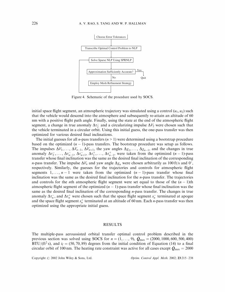
The procedure for using SOCS is as follows. It is necessary to specify an initial nodedistribution (mesh), i.e. an initial set of time points at which to compute the optimal solution,for each phase of the problem. Furthermore, at each node it is necessary to specify a guess forthe state and control and for each phase it is necessary to specify a guess for the optimizationparameters. Finally, it is necessary to specify differential equation accuracy tolerances andoptimization convergence tolerances. The optimal solution is then computed using all of theaforementioned information. If, upon convergence, the differential equation accuracy toleranceis not met, a mesh refinement strategy is invoked that adds nodes to form a denser mesh; theoptimization problem is then solved on the refined mesh. This process of solving theoptimization problem and refining the mesh is repeated until the user-specified accuracytolerances are met. A schematic of the aforementioned procedure is shown in Figure 4.

Due to the complexity of this problem, it was a great challenge to determine initial guesses forthe trajectory and the optimization parameters. Before proceeding to the multiple-pass transfer,initial guesses were determined for the one-pass transfer as follows. The impulse DV1 and changein true anomaly Dtþ1 were chosen such that the initial space flight segment would terminate at analtitude of 60 nm (the initial yaw angle w1 was set to zero). Then, using the state at the end of the



initial space flight segment, an atmospheric trajectory was simulated using a control ðu1; u2Þ suchthat the vehicle would descend into the atmosphere and subsequently re-attain an altitude of 60nm with a positive flight path angle. Finally, using the state at the end of the atmospheric flightsegment, a change in true anomaly Dt�2 and a circularizing impulse DV2 were chosen such thatthe vehicle terminated in a circular orbit. Using this initial guess, the one-pass transfer was thenoptimized for various desired final inclinations.

The initial guesses for all n-pass transfers (n > 1) were determined using a bootstrap procedurebased on the optimized ðn� 1Þ-pass transfers. The bootstrap procedure was setup as follows.The impulses DV1; . . . ; DVn�1; DVnþ1; the yaw angles Dw1; . . . ; Dwn�1; and the changes in trueanomaly Dt�2 ; . . . ; Dt

�n�1; Dt

�nþ1; Dt

þ1 ; . . . ; Dt

þn�1; were taken from the optimized ðn� 1Þ-pass

transfer whose final inclination was the same as the desired final inclination of the correspondingn-pass transfer. The impulse DVn and yaw angle Dwn were chosen arbitrarily as 100 ft/s and 08;respectively. Similarly, the guesses for the trajectories and controls for atmospheric flightsegments 1; . . . ; n� 1 were taken from the optimized ðn� 1Þ-pass transfer whose finalinclination was the same as the desired final inclination for the n-pass transfer. The trajectoriesand controls for the nth atmospheric flight segment were set equal to those of the ðn� 1Þthatmospheric flight segment of the optimized ðn� 1Þ-pass transfer whose final inclination was thesame as the desired final inclination of the corresponding n-pass transfer. The changes in trueanomaly Dt�n ; and Dtþn were chosen such that the space flight segment s�n terminated at apogeeand the space flight segment sþn terminated at an altitude of 60 nm. Each n-pass transfer was thenoptimized using the appropriate initial guess.

RESULTS

The multiple-pass aeroassisted orbital transfer optimal control problem described in theprevious section was solved using SOCS for n ¼ ð1; . . . ; 9Þ; ’QQmax ¼ ð2000; 1000; 600; 500; 400ÞBTU/(ft2 s), and if ¼ ð50; 70; 89Þ degrees from the initial condition of Equation (14) to a finalcircular orbit of 100 nm. The heating rate constraint was active for all cases except ’QQmax ¼ 2000

Transcribe Optimal Control Problem to NLP

Choose Error Tolerances

Solve Sparse NLP Using SPRNLP

Approximation Sufficiently Accurate? Yes

QuitNo

Employ Mesh Refinement Strategy

Figure 4. Schematic of the procedure used by SOCS.



BTU/(ft2 s), i.e. the case ’QQmax ¼ 2000 BTU/(ft2 s) was equivalent to a problem with noconstraint on ’QQ:

The minimum total impulse, DVmin; is shown in Figures 5–7 as a function of n for the differentvalues of ’QQmax: When the heating rate is unconstrained the multiple-pass transfer offers only a

n

∆Vm

in (f

t/se

c)

Qmax = 2000 BTU/(ft2 sec)

1 2 3 4 5 6 7 8 95200

5400

5600

5800

6000

6200.

Qmax = 1000 BTU/(ft2 sec).




Figure 5. DVmin vs n for if ¼ 508:

n

∆Vm

in (f

t/se

c)


1 2 3 4 5 6 7 8 9

8000

7600

7200

6800

6400

.








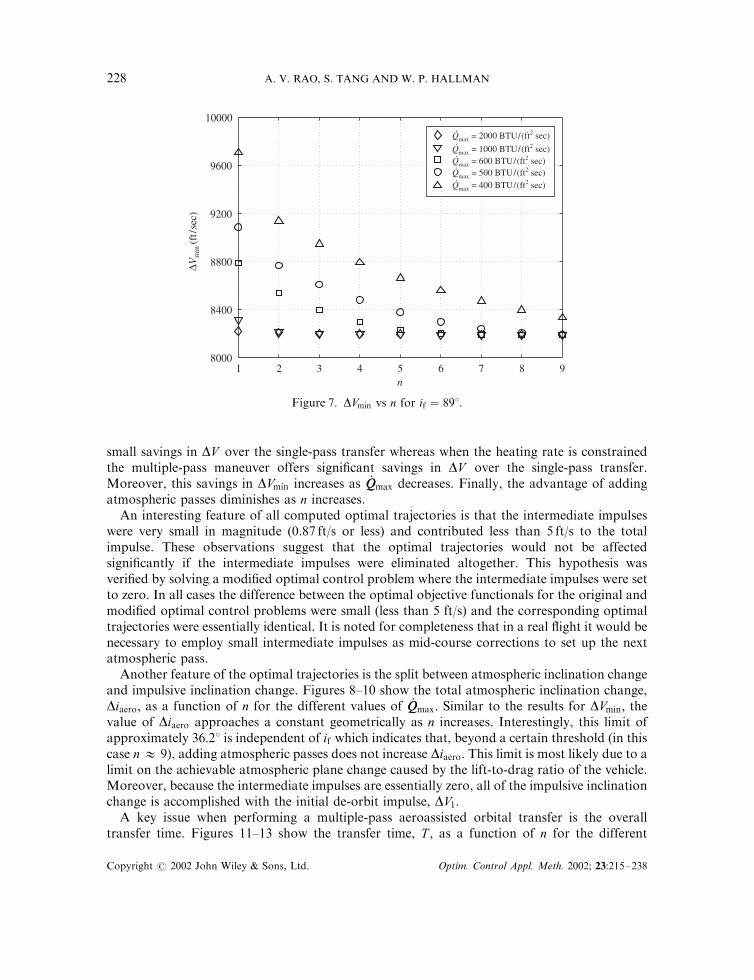
small savings in DV over the single-pass transfer whereas when the heating rate is constrainedthe multiple-pass maneuver offers significant savings in DV over the single-pass transfer.Moreover, this savings in DVmin increases as ’QQmax decreases. Finally, the advantage of addingatmospheric passes diminishes as n increases.

An interesting feature of all computed optimal trajectories is that the intermediate impulseswere very small in magnitude (0.87 ft/s or less) and contributed less than 5 ft/s to the totalimpulse. These observations suggest that the optimal trajectories would not be affectedsignificantly if the intermediate impulses were eliminated altogether. This hypothesis wasverified by solving a modified optimal control problem where the intermediate impulses were setto zero. In all cases the difference between the optimal objective functionals for the original andmodified optimal control problems were small (less than 5 ft/s) and the corresponding optimaltrajectories were essentially identical. It is noted for completeness that in a real flight it would benecessary to employ small intermediate impulses as mid-course corrections to set up the nextatmospheric pass.

Another feature of the optimal trajectories is the split between atmospheric inclination changeand impulsive inclination change. Figures 8–10 show the total atmospheric inclination change,Diaero; as a function of n for the different values of ’QQmax: Similar to the results for DVmin; thevalue of Diaero approaches a constant geometrically as n increases. Interestingly, this limit ofapproximately 36:28 is independent of if which indicates that, beyond a certain threshold (in thiscase n � 9), adding atmospheric passes does not increase Diaero: This limit is most likely due to alimit on the achievable atmospheric plane change caused by the lift-to-drag ratio of the vehicle.Moreover, because the intermediate impulses are essentially zero, all of the impulsive inclinationchange is accomplished with the initial de-orbit impulse, DV1:

A key issue when performing a multiple-pass aeroassisted orbital transfer is the overalltransfer time. Figures 11–13 show the transfer time, T ; as a function of n for the different

2n

∆Vm

in (f

t/se

c)


1 3 4 5 6 7 8 98000

8400

8800

9200

9600

10000.








values of ’QQmax: It is seen for all cases that the transfer time for n ¼ 1 is approximately6 h. Furthermore, for a particular value of n the transfer time is the shortest when ’QQ isunconstrained.

One of the purported advantages of aeroassisted orbital transfer is the savings in requiredimpulse over non-coplanar two-impulse (Hohmann-type) and three-impulse (bi-elliptic) all-propulsive transfers [26]. Table II shows the minimum DV requirements for these all-propulsive

2n

∆iae

ro (d

eg)


1 3 4 5 6 7 8 920

24

28

32

36

40

.





Figure 8. Total atmospheric inclination change, Diaero vs n for if ¼ 508:

2n

∆iae

ro (d

eg)


1 3 4 5 6 7 8 920

24

28

32

36

40

.








transfers from GEO to 100 nm altitude circular orbit for final inclinations of 50, 70, and 898 (thethree impulse bielliptic transfer were constrained to be less than 300 days). It can be seen in allcases that the aeroassisted orbital transfer offers substantial savings in DV over either of theseall-propulsive transfers.

2n

∆iae

ro (d

eg)


1 3 4 5 6 7 8 920

24

28

32

36

40

.






n

T (

hr)


1 2 3 4 5 7 8 90

6

6

12

18

24

30

36

42

48.





Figure 11. Transfer time, T vs n for if ¼ 508:



The case n ¼ 4; ’QQmax ¼ 400 BTU/(ft2 s), and if ¼ 898 is now used to illustrate the mainfeatures common to all of the computed optimal trajectories. Results for h; v; and i are shown inFigures 14 and 15. It can be seen that the speed at each atmospheric exit is equal to the speed atthe subsequent atmospheric entry. This behaviour is expected since the entry and exit altitudes

n

T (

hr)


1 2 3 4 5 7 8 90

6

6

12

18

24

30

36

42

48.






n

T (

hr)


1 2 3 4 5 7 8 90

6

6

12

18

24

30

36

42

48.








are equal and there is essentially no change to the Keplerian orbit during the intervening spaceflight segment. Moreover, the decrease in speed during the final atmospheric pass is significantlylarger than the decrease in speed during any of the earlier atmospheric passes. The reason forthis larger speed decrease is that the velocity is lowest during the final atmospheric pass andthereby permits deeper atmospheric penetration. Similarly, the inclination at atmospheric exitand the subsequent atmospheric entry are equal and the inclination change during the lastatmospheric pass is significantly larger than the inclination change during any of the earlieratmospheric passes.

Results for g are shown in Figure 16. A structure common to all optimal trajectories is that his nearly symmetric with respect to g for all but the final atmospheric pass. During the finalatmospheric flight segment it is seen that two flight conditions occur simultaneously. First, thevehicle achieves an altitude change at constant flight path angle. Second, (see Figure 20) thevehicle flies along its heating rate limit. These two flight conditions together demonstrate that,during the final atmospheric segment, the vehicle is flying along an equilibrium glide condition.

v (ft /sec) × 1000

h (n

m)

1st Atmospheric Pass2nd Atmospheric Pass3rd Atmospheric Pass4th Atmospheric Pass

24 26 28 32 3430

30

40

50

60

70

80

Figure 14. h vs v for n ¼ 4; ’QQmax ¼ 400BTU/(ft2 s), and if ¼ 898:

Table II. Results of two-impulse and three-impulseall-propulsive transfers from GEO to 100 nm circular

orbit for if = 50, 70, and 898

DV (ft/s) DV (ft/s)if (deg) (two-burn) (three-burn)

50 15 800 14 79570 17 600 14 82089 19 260 14 840



The equilibrium glide condition during the final atmospheric flight segment was common to allof the optimal trajectories.

Typical control profiles s and CL are shown in Figures 17–19. It can be seen from Figure 19that the constraint on CL is active during the entirety of the first atmospheric flight segment.

� (deg)

h (n

m)


-5 -4 -3 -2 -1 0 1 2 3 4 530

40

50

60

70

80

Figure 16. h vs g for n ¼ 4; ’QQmax ¼ 400BTU/(ft2 s), and if ¼ 898

i (deg)

h (n

m)


55 65

70

75

80

85 9530

40

50

60

Figure 15. h vs i for n ¼ 4; ’QQmax ¼ 400BTU/(ft2 s), and if ¼ 898:



Furthermore, it can be seen by examining Figures 17 and 18 simultaneously that a reversal inbank angle rate always occurs when the vehicle reaches a minimum altitude.

The value of ’QQ is shown in Figure 20 where ’QQ is plotted alongside the time from atmosphericentry, Dtentry: It can be seen that ’QQ rides the path constraint upper bound during the final

30

40

50

60

70

80

h (n

m)

∆tentry (s)


0 200 400 600 800 1000 1200

Figure 18. h vs Dtentry for n ¼ 4; ’QQmax ¼ 400BTU/(ft2 s), and if ¼ 898:

� (d

eg)

∆tentry (s)

1st Atmospheric Pass

2nd Atmospheric Pass3rd Atmospheric Pass4th Atmospheric Pass

-180

-160

-140

-120

-100

-80

-60

0 200 400 600 800 1000 1200

Figure 17. s vs Dtentry for n ¼ 4; ’QQmax ¼ 400BTU/(ft2 s), and if ¼ 898:



atmospheric flight segment but appears to only touch the constraint during all earlieratmospheric flight segments. While the conditions derived in Reference [27] can be used to ruleout the existence of a touch point in the current application, a rigorous analysis is beyond thescope of this paper.

Q (

BT

U/(

ft2

s))

∆tentry (s)


00 600 800 1000 1200

100

200

200

300

400

400

500

Figure 20. ’QQ vs Dtentry for n ¼ 4; ’QQmax ¼ 400BTU/(ft2 s), and if ¼ 898:

CL

∆tentry (s)

1st Atmospheric Pass2nd Atmospheric Pass3rd Atmospheric Pass

4th Atmospheric Pass

0.1

0.2

0.3

0.4

0.5

00 200 400 600 800 1000 1200

Figure 19. CL vs Dtentry for n ¼ 4; ’QQmax ¼ 400BTU/(ft2 s), and if ¼ 898:



CONCLUSIONS

A numerical optimization study of multiple-pass aeroassisted orbital transfer has beenperformed using a direct transcription method. The objective has been to provide highlyaccurate solutions to the problem of minimum-impulse heat-rate-limited large plane changemultiple-pass aerogliding maneuvers for a high lift-to-drag vehicle from geostationary orbit tolow Earth orbit. The minimum-impulse performance has been assessed as a function of thenumber of atmospheric passes, the maximum allowable heating rate, and the desired terminalinclination.

The results show that the multiple-pass aeroassisted orbital transfer offers little to no savingsin total impulse over the single-pass transfer when the heating rate is unconstrained but offerssignificant savings in total impulse when the heating rate is constrained. A useful feature of theapproach developed here is that the optimal split between atmospheric and impulsive inclinationchange is determined. Furthermore, it was found that there is a limit to the total amount ofinclination change performed during atmospheric flight. Finally, a particular case of a four-passtransfer was used to illustrate the main features common to all of the optimal trajectories.

NOMENCLATURE

CD coefficient of dragCD0

zero-lift coefficient of dragCL coefficient of liftCL;a derivative of CL with respect to a; deg�1

CL;max maximum coefficient of liftD drag acceleration, ft/s2

g0 gravitational acceleration at sea level, ft/s2

h altitude, ft and nmha apogee altitude, nmhf altitude of spacecraft in final circular orbit, ft and nmhp perigee altitude, nmi inclination, degIsp specific impulse, sK drag polar parameterL lift acceleration, ft/s2

m vehicle mass, slugm0 initial vehicle mass, slugme final vehicle mass, slugq dynamic pressure, lb/ft2

’QQ heating rate, BTU/(ft2 s)’QQmax maximum stagnation point heating rate, BTU/(ft2 s)r radius, ftr inertial position, ftRe radius of Earth, ftS vehicle reference area, ft2



ACKNOWLEDGEMENTS

The authors gratefully acknowledge the United States Air Force Space and Missile Systems Center forsupporting this research. Furthermore, the authors acknowledge Twain Summerset for his role as technicalmonitor and his helpful insights throughout the course of this work. Finally, the authors acknowledge AlanJenkin, Steven Hast, and Ryan Noguchi of The Aerospace Corporation for their helpful comments andsuggestions in preparing this manuscript.

REFERENCES

1. Walberg GD. A survey of aeroassisted orbit transfer. Journal of Spacecraft and Rockets 1985; 22(1):3–17.2. Mease KD. Optimization of aeroassisted orbital transfer: current status. Journal of the Astronautical Sciences 1988;

36(1/2):7–33.3. Hull DG, Giltner JM, Speyer JL, Mapar J. Minimum energy-loss guidance for aeroassisted orbital plane change.

Journal of Guidance, Control, and Dynamics 1985; 8(4):487–493.4. Melamed N, Calise AJ. Evaluation of an optimal-guidance for an aero-assisted orbit transfer. Journal of Guidance,

Control, and Dynamics 1995; 18(4):718–722.5. Seywald H. Variational solutions for the heat-rate-limited aeroassisted orbital transfer problem. Journal of Guidance,

Control, and Dynamics 1996; 19(3):686–692.6. Lee JY, Hull DG. Maximum orbit plane change with heat-transfer-rate considerations. Journal of Guidance, Control,

and Dynamics 1990; 13(3):492–497.7. Vinh NX, Hanson JM. Optimal aeroassisted return from high earth orbit with plane change. Acta Astronautica

1985; 12(1):11–25.

s� space flight segment before impulsive maneuversþ space flight segment after impulsive maneuvert time, sT orbital transfer time, sv inertial velocity, ft/sv speed, ft/sve circular orbit speed at surface of the Earth, ft/sa angle of attack, degamax maximum angle of attack, degw Euler yaw angle of impulsive thrust maneuver, ft/sDtentry Time since atmospheric entry, sDV magnitude of impulsive thrust maneuver, degDt change in true anomaly, degg flight path angle, degm gravitational parameter, ft3/s2

n true anomaly, dego argument of perigee, degO right ascension of ascending node, degy longitude angle, degc heading angle, degr air density, slug/ft3

re air density at sea level, slug/ft3

s bank angle, degf latitude angle, degt true anomaly, deg



8. Vinh NX, Ma D-M. Optimal multiple-pass aeroassisted plane change. Acta Astronautica 1990; 21(11/12):749–758.9. Hargraves CR, Paris SW. Direct trajectory optimization using nonlinear programming and collocation. Journal of

Guidance, Control, and Dynamics 1987; 10(4):338–342.10. Enright PJ, Conway BA. Optimal finite-thrust spacecraft trajectories using collocation and nonlinear programming.

Journal of Guidance, Control, and Dynamics 1991; 14(5):981–985.11. Herman AL, Conway BA. Direct optimization using collocation based on high-order gauss-lobatto quadrature

rules. Journal of Guidance, Control, and Dynamics 1996; 19(3):592–599.12. Betts JT. Survey of numerical methods for trajectory optimization. Journal of Guidance, Control, and Dynamics 1998;

21(2):193–207.13. Vlases WG, Paris SW, Lajoie RM, Martens PJ, Hargraves CR. Optimal trajectories by implicit simulation. Boeing

Aerospace and Electronics, Technical Report WRDC-TR-90-3056, Wright-Patterson Air Force Base, 1990.14. Schnepper K. PROMIS Software User Manual. Schwerpunktprogramm der Deutschen Forschungsgemeinschaft:

Andwendungsbezogene Optimierung and Steuerung, Report 509, Institute of Flight Mechanics and Control,University of Stuttgart, Stuttgart, Germany, 1994.

15. Betts JT, Huffman WP. Sparse optimal control software, SOCS. Mathematics and Engineering Analysis LibraryReport. MEA-LR-085, 15 July 1997, Boeing Information and Support Services, P.O. Box 3797, Seattle, WA,98124-2297.

16. Zimmermann F, Calise AJ. Numerical optimization study of aeroassisted orbital transfer. Journal of Guidance,Control and Dynamics 1998; 21(1):127–133.

17. Hanson JM. Combining propulsive and aerodynamic maneuvers to achieve optimal orbital transfer. Journal ofGuidance, Control, and Dynamics 1985; 12(5):732–738.

18. Huffman WP. An analytic propagation method for low earth orbits. Internal Document. The AerospaceCorporation, El Segundo, CA, November 1981.

19. Vinh NX, Busemann A, Culp RD. Hypersonic and planetary entry flight mechanics. University of Michigan Press,Ann Arbor, MI, 1980.

20. Brenan KE. A Smooth Approximation to the GTS 1962 Standard Atmosphere Model. Aerospace ATM 82-(2468-04)-7, 21 May 1982.

21. Detra RW, Kemp NH, Riddell FR. Addendum to heat transfer to satellite vehicles re-entering the atmosphere. JetPropulsion 1957; 27:1256–1257.

22. Brenan KE, Campbell SL, Petzold JR. Numerical Solution of Initial-Value Problems in Differential AlgebraicEquations. Elsevier Sciences Publishing: New York, 1989.

23. Brenan KE. Differential-algebraic equations issues in the direct transcription of path constrained optimal controlproblems. Annals of Numerical Mathematics 1994; 1:247–263.

24. Betts JT, Frank PD. A sparse nonlinear optimization algorithm. Journal of Optimization Theory and Applications1994; 82(3):519–541.

25. Jansch C, Schnepper K, Well, K. Multi-phase trajectory optimization methods with applications to hypersonicvehicles. Schwerpunktprogramm der Deutchen Forschungsgemeinschaft: Anwendungsbezogene Optimierung andSteuerung, Report 419, Institute of Flight Mechanics and Control, University of Stuttgart, Stuttgart, Germany,1994.

26. Chobotov VA. Orbital Mechanics. American Institute of Aeronautics and Astronautics: Washington, DC, 1991.27. Seywald H, Cliff EM. On the existence of touch points for first-order state inequality constraints. Optimal Control

Applications and Methods 1996; 17:357–366.



Numerical optimization study of multiple-pass...

Documents

Transcript of Numerical optimization study of multiple-pass...