Numerical Models on Innovative Steel Hollow Section Joints ...

Numerical Models on Innovative Steel Hollow Section

Joints for Truss Girders using Laser Cut Technology

Bernardo Segurado Correia Pita Dias

Dissertation to obtain the Master of Science Degree in

Civil Engineering

Supervisors: Professor Luís Manuel Calado de Oliveira Martins

Professor Jorge Miguel Silveira Filipe Mascarenhas Proença

Examination Committee

Chairperson: Professor António Manuel Figueiredo Pinto da Costa

Supervisor: Professor Luís Manuel Calado de Oliveira Martins

Members of the Committee: Professor Pedro António Martins Mendes

October, 2017

To my mother

i

Acknowledgements

My first acknowledgment is to my supervisors: Professor Luis Calado and Professor Jorge Proença. My

unmeasurable thanks to Professor Luís Calado for constantly challenging me and guiding me throughout

this project, always with a word of wisdom and keen advice, and to Professor Jorge Proença for inviting

me to the project. I am also grateful to Professor Carlo Castiglioni for accepting to be my supervisor in

Politecnico di Milano.

A special word to my Parents for having supported me all the way and giving me all of the freedom a

son could ask for.

Last, but not least, a word of gratitude to all my friends for making me feel lucky, in special to Inês for

the long hours of study and work that we shared.

iii

Resumo

A necessidade de reduzir a complexidade de conexões entre elementos metálicos é clara. LASTEICON

é um projeto Europeu que visa o desenvolvimento de ligações metálicas por corte laser, cujo objetivo

é redução da quantidade de soldadura e a eliminação da utilização de placas gusset em ligações viga-

coluna. A possibilidade de utilização da tecnologia para ligações metálicas em treliças é o ponto de

partida desta dissertação.

O principal objetivo é a construção dos modelos numéricos e a realização da análise paramétrica de

diferentes tipos de nós tirando partido da tecnologia de corte laser. O corte preciso desta tecnologia

permite abrir ranhuras nos perfis da corda, possibilitando a entrada dos elementos diagonais e verticais,

constituindo uma alternativa inovadora de ligação.

Os resultados dos modelos numéricos das diferentes ligações foram comparados em termos de

distribuição de tensões e sugerem uma redução tensão máxima de Von Mises até 10% em alguns

casos.

A análise paramétrica revela uma maior sensibilidade deste tipo de conexões para valores inferiores

de espessura da corda. Adicionalmente, os casos estudados sugerem a possibilidade do mesmo

comportamento de ligações tradicionais para menores espessuras de corda, no caso de utilização de

corte laser.

Calibração, validação do modelo e confirmação das conclusões será possível com a realização futura

dos testes experimentais.

Palavras-chave:

Corte Laser; Estruturas de Aço; Análise numérica; Ligações tubulares

v

Abstract

This thesis is framed by LASTEICON EU research project on the development of steel joints using laser

cut technology aimed at enhancing the economy and sustainability of I-beam-to-CHS-column

connections fabrication, by eliminating stiffener plates and reducing the amount of welding. The

extendibility of laser cut technology to steel truss girder applications is the kick-off for this dissertation.

Based on numerical and parametric analysis of different steel truss girder joint typologies using laser

cut technology, the main goal is to retrieve conclusions about its feasibility and give indication to its

experimental work package.

Taking advantage of laser cut and the possibility of opening precise slots on the face of the chord, the

joint typologies studied consisted on the prolongation of the bracing elements of the truss girder to the

inside of the chord. These were analysed and stress distribution on the connection was evaluated.

Global rigidity of the truss girder is also under interest. Numerical analysis suggests an increase of

performance in laser cut joints, in some cases up to 10% reduction of maximum Von Mises stress.

Local study shows that it is possible to have similar behaviour of traditional joints with lower values of

thickness of the chord if Laser Cut Technologies joints are used. In addition, parametric analysis suggest

a higher improvement in structural behaviour for lower values of chord thickness.

Keywords

Laser cut; Steel Truss girders; Numerical analysis; Steel Joints

vii

Contents

1. Introduction .......................................................................................................................................... 1

1.1 Framework ..................................................................................................................................... 1

1.2 Project LASTEICON ...................................................................................................................... 1

1.3 Dissertation framework .................................................................................................................. 3

1.3.1 IST Project .............................................................................................................................. 3

1.3.2 Objectives ............................................................................................................................... 5

1.3.3 Organization of the dissertation .............................................................................................. 5

2. Literature Review ................................................................................................................................. 7

2.1 Introduction .................................................................................................................................... 7

2.2 New developments ........................................................................................................................ 7

2.3 Laser Cut Technology (LCT) ......................................................................................................... 8

2.4 Hollow section profiles ................................................................................................................. 10

2.5 Design Regulations ..................................................................................................................... 11

2.5.1 Strength Criteria ................................................................................................................... 14

2.5.1.1 Failure Modes .................................................................................................................... 14

2.5.1.2 Welds ................................................................................................................................. 17

2.5.2 Deformation Limit Criteria ..................................................................................................... 17

2.6 Numerical Modelling .................................................................................................................... 18

2.6.1 Model types .......................................................................................................................... 19

2.6.2 Boundary Conditions ............................................................................................................ 22

2.6.3 Weld modelling ..................................................................................................................... 24

2.6.4 Elements ............................................................................................................................... 25

2.6.5 Mesh ..................................................................................................................................... 25

2.6.6 Material ................................................................................................................................. 26

3. Joint typologies and Substructures ................................................................................................... 29

3.1 Joint typologies ............................................................................................................................ 29

3.2 Substructures .............................................................................................................................. 34

viii

4. Numerical Model ................................................................................................................................ 37

4.1 Model type ................................................................................................................................... 37

4.2 Boundary Conditions and Non-linearity ....................................................................................... 39

4.3 Mesh sensibility analysis ............................................................................................................. 41

4.4 Validation ..................................................................................................................................... 44

5. Numerical Study ................................................................................................................................ 45

5.1 Nodes of interest ......................................................................................................................... 45

5.2 Substructure A ............................................................................................................................. 48

5.2.1 Node NA-1 ............................................................................................................................ 48

5.2.2 Node NA-2 ............................................................................................................................ 52

5.2.3 Global behaviour of Substructure A ..................................................................................... 53

5.3 Substructure B ............................................................................................................................. 55

5.3.1 Node NB-1 ............................................................................................................................ 55

5.3.2 Node NB-2 ............................................................................................................................ 56

5.3.3 Global behaviour of substructure B ...................................................................................... 58

5.4 General discussion ...................................................................................................................... 59

6. Parametric analysis ........................................................................................................................... 61

6.1 Parametric analysis of the bracing thickness .............................................................................. 62

6.2 Parametric analysis of the chord thickness ................................................................................. 64

6.3 Local behaviour ........................................................................................................................... 65

7. Conclusions and Future Studies ....................................................................................................... 73

7.1 Conclusions ................................................................................................................................. 73

7.2 Future Studies ............................................................................................................................. 74

References ............................................................................................................................................ 77

ix

List of Figures

Figure 1 - Prototype of I-shaped beam to circular column connection using Laser Cut Technology [6]. 2

Figure 2 - Diagram Flow of the work package between IST and other partners..................................... 3

Figure 3 - Prototype of Laser Cut Technology connection using open section beams ........................... 4

Figure 4 - Diagram flow of production responsibility ............................................................................... 5

Figure 5 - Vierendeel, square bird-beak and diamond bird-beak joints [21] ........................................... 8

Figure 6 - Detail of Laser Cut Technology benefit in terms of cutting edge precision [6]........................ 9

Figure 7 - Proportional factors of total steel frame cost [29] ................................................................. 10

Figure 8 - Examples of steel tubular connections using intermediate plate (left) and directly welded to

the profiles (right) [28] ............................................................................................................................ 11

Figure 9 - Eccentricities at joints [8] ...................................................................................................... 12

Figure 10- Uniplanar joints [8] ............................................................................................................... 13

Figure 11 - Multiplanar joints [8] ............................................................................................................ 13

Figure 12 - Failure modes for RHS chord and brace members ............................................................ 15

Figure 13 - CHS K joint and CHS T joint geometry [34] ........................................................................ 16

Figure 14 - out of plane displacement (chord surface deformation) [38] ............................................. 17

Figure 15 - Deformation Limit Criteria [34] ............................................................................................ 18

Figure 16 - Example of Truss Space Model [47] (adapted) .................................................................. 19

Figure 17 - Example of combined model with beam and shell elements [47] (adapted) ...................... 20

Figure 18 - Example of model with isolated truss girder joint [47] (adapted) ........................................ 20

Figure 19 - Comparing load-displacement curves for 2D and 3D models [47] ..................................... 21

Figure 20 - Comparing load-displacements diagrams for the different models [47] ............................. 21

Figure 21 - Modelling eccentricities for overlap and gap joints [47] ...................................................... 22

Figure 22 - Joint modelling assumptions for gap and overlap cases [33] ............................................. 22

Figure 23 - K-joints with single (left) and double (right) boundary conditions[51]. ................................ 23

Figure 24 - K-joint models with different boundary conditions [43] ....................................................... 23

Figure 25 - Different K-joint boundary conditions [56] ........................................................................... 24

Figure 26 - Modelling procedure combining linear and planar elements [56] ....................................... 24

Figure 27 - Limit angles for quadrilateral elements in FEA [41] ............................................................ 26

Figure 28 - Eurocode suggestion for modelling material behaviour [70] ............................................... 27

Figure 29 - Detail of joint typology "base" ............................................................................................. 30

Figure 30 - 3D views of the joint typology "base" .................................................................................. 30

Figure 31 - Detail of joint typology "Cut1" .............................................................................................. 31

Figure 32 - 3D views of the joint typology "Cut1" .................................................................................. 31

Figure 33 - Detail of joint typology "Cut2" .............................................................................................. 32

x

Figure 34 - 3D views of the joint typology "Cut2" .................................................................................. 32

Figure 35 - 3D detail of bracing elements in joint typology "Cut2" ........................................................ 32

Figure 36 - Detail of alternative joint typology with plate ....................................................................... 33

Figure 37 - 3D views of alternative joint typology with plate ................................................................. 33

Figure 38 - Detail of alternative joint typology ....................................................................................... 33

Figure 39 - Substructure A .................................................................................................................... 34

Figure 40 - Substructure B .................................................................................................................... 34

Figure 41 - Load-Displacement curves for substructure A and substructure B .................................... 35

Figure 42 - Profile cross-sections of substructure A ............................................................................. 36

Figure 43 - Profile cross-sections of substructure B ............................................................................. 36

Figure 44 - Representation of failure mode for substructure A ............................................................. 36

Figure 45 - Representation of failure mode for substructure B ............................................................. 36

Figure 46 - Bi-linear constitutive law ..................................................................................................... 38

Figure 47 - Abaqus view of the truss modelled with the shell joint ........................................................ 39

Figure 48 - Detail of the interaction between linear and planar elements ............................................. 40

Figure 49 - Load and displacement convergence when increasing the number of elements ............... 41

Figure 50 - Comparison of load convergence with CPU time when increasing the number of elements

............................................................................................................................................................... 42

Figure 51 - Maximum Von Mises stress value at the joint used for the mesh sensibility test ............... 44

Figure 52 - Location of NA-1 on substructure A .................................................................................... 46

Figure 53 - Substructure A modelled with shell elements on NA-1 ....................................................... 46

Figure 54 - Location of NA-2 on substructure A .................................................................................... 46

Figure 55 - Substructure A modelled with shell elements on NA-2 ....................................................... 46

Figure 56 - Location of NB-1 on substructure B .................................................................................... 47

Figure 57 - Substructure B modelled with shell elements on NB-1 ....................................................... 47

Figure 58 - Location of NB-2 on substructure B .................................................................................... 47

Figure 59 - Substructure B modelled with shell elements on NB-2 ....................................................... 47

Figure 60 - Substructure A with shell elements at the nodes ................................................................ 53

Figure 61 - Substructure A with rigid nodes .......................................................................................... 53

Figure 62 - Substructure A with pinned nodes ...................................................................................... 54

Figure 63 - Load-displacement diagram for the different joint typologies in substructure A ................. 54

Figure 64 - Substructure B with shell elements at the nodes ................................................................ 58

Figure 65 - Substructure B with rigid nodes .......................................................................................... 58

Figure 66 - Substructure B with pinned nodes ...................................................................................... 59

Figure 67 - Load-displacement diagram for the different joint typologies in substructure B ................. 59

Figure 68 - Node of interest used in the sensibility analysis ................................................................. 61

Figure 69 - Brace and chord thickness representation ......................................................................... 62

Figure 70 - Evolution of the difference in terms of 𝜎𝑉𝑀𝑚𝑎𝑥 from cut1 and cut2 to base case when

increasing brace thickness .................................................................................................................... 63

xi

Figure 71 - Evolution of the difference in terms of 𝜎𝑉𝑀𝑚𝑎𝑥from cut1 and cut2 to base case when

increasing chord thickness .................................................................................................................... 64

Figure 72 - Deformation of base type for tb=4mm ................................................................................. 65

Figure 73 - Deformation of cut1 type for tb=4mm .................................................................................. 66

Figure 74 - Deformation of cut2 type for tb=4mm .................................................................................. 66

Figure 75 - Representation of Nj-1 and Nj-2 for the local study ............................................................ 67

Figure 76 - Load-displacement curve for Nj-1 (tc=3mm) ....................................................................... 68






Figure 82 - Load-displacement curve for base and cut1 cases at nj-1 ................................................. 71



Figure 85 - Load-displacement curve for base and cut2 at nj-2 ............................................................ 72

xiii

List of Tables

Table 1 - Comparison between cutting methods [6] ................................................................................ 9

Table 2 - Decision table for considering bending moments in truss design [33] ................................... 13

Table 3 - Geometrical range of validity for CHS T and K joints [34]...................................................... 16

Table 4 - Design formulae for CHS K and T joints [34] ......................................................................... 16

Table 5 - Material characteristics .......................................................................................................... 39

Table 6 - Mesh sensibility analysis for substructure A .......................................................................... 41

Table 7 - Mesh sensibility study for shell elements ............................................................................... 43

Table 8 - Mesh sensibility test results ................................................................................................... 44

Table 9 - Comparison of joint typologies for NA-1 in terms of Von Mises Stress ................................. 48

Table 10 - Top view of the comparison detail of Von Mises stress distribution on the top face of the

chord for the different joint typologies ................................................................................................... 49

Table 11 - Bottom view of the comparison detail of Von Mises stress distribution on the bottom face of

the chord for the different joint typologies ............................................................................................. 50

Table 12 - Comparison of joint typologies for NA-1 in terms of Von Mises Stress (inside view) .......... 51

Table 13 - Comparing results for the different joint typologies on NA-1 ............................................... 51

Table 14 - Comparison of joint typologies for NA-2 in terms of Von Mises Stress ............................... 52

Table 15 - Comparing results for the different joint typologies on NA-2 ............................................... 53

Table 16 - Comparison of joint typologies for NB-1 in terms of Von Mises Stress .............................. 55

Table 17 - Comparing results for the different joint typologies on NB-1 ............................................... 56

Table 18 - Comparing results for the different joint typologies on NB-2 ............................................... 56

Table 19 - Comparing results for the different joint typologies on NB-2 for P=110 kN ......................... 56

Table 20 - Comparison of joint typologies for NB-2 in terms of Von Mises Stress ............................... 57

Table 21 - Results on the joint typologies behaviour by varying brace thickness ................................. 62

Table 22 - Results on the joint typologies behaviour by varying chord thickness ................................. 64

xv

List of symbols

𝐴0 chord cross sectional area

𝐸 modulus of elasticity of steel

𝐸𝑡 tangent modulus of elasticity of steel

𝐹𝑤,𝐸𝑑 design resultant of all the forces transmitted by the weld per unit length

𝐹𝑤,𝑅𝑑 design weld resistance per unit length

𝑁𝑖 axial force resultant in member i

𝑀0,𝐸𝑑 design value of bending moment at chord

𝑊𝑒𝑙,0 elastic section modulus of the chord

𝑁𝑖,𝑅𝑑 design axial resistance of member i

𝑄𝑓 chord stress function

𝑑0 chord diameter

𝑑𝑖 member i diameter

𝑒 eccentricity at the joint

𝑓𝑦0 yield strength of the chord

𝑓𝑦𝑖 yield strength of member i

𝑔 gap between the brace members

ℎ𝑜 in-plane depth of the chord

𝑡0 chord thickness

𝑡𝑏 brace thickness for parametric analysis (see figure 69)

𝑡𝑐 chord thickness for parametric analysis(see figure 69)

𝑡𝑖 member i thickness

𝑛𝑝 ratio between 𝜎0,𝐸𝑑 and 𝑓𝑦0, by a safety coefficient 𝛾𝑀5

𝛽 the ratio of the mean diameter or width of the brace members, to that of the chord

𝛾 ratio of the chord width or diameter to twice its wall thickness

xvi

𝛾𝑀5 safety coefficient

𝛾𝑠 steel mass density

𝜕 displacement

𝜀 engineering strain

𝜀𝑡𝑟𝑢𝑒 true strain

𝜃𝑖 angle between brace i and chord

𝜇𝑖 the ratio of the diameter to the thickness of member i

𝑣 poisson coeficient

𝜎 engineering stress

𝜎0,𝐸𝑑 maximum compressive stress in the chord at a joint

𝜎𝑡𝑟𝑢𝑒 true stress

𝜎𝑉𝑀𝑚𝑎𝑥 maximum Von Mises stress

1

1. Introduction

1.1 Framework

EU can trace its origins to the creation of European Coal and Steel Community, which from the early

50’s had as a primary goal to unify countries after World War II, by creating a common market for its

members of Coal and Steel. Not only it contributed to economic growth but also it worked as the

foundation for the European Community as we know today. It was already at the time recognizable the

importance of these materials and this relevance is still present in nowadays investigation and research.

At the European Level, the Research Fund for Coal and Steel (RFCS) is the entity responsible for this

and it contributes to the sustainable development of the material and technology by funding over

€50million euros every year in projects that aim at increasing safety and competitive edge in the industry

[1].

To these days, steel is still considered a European Industry with 500 production sites between 23

Member States. Today, EU is responsible for 177 million tonnes of steel a year, representing 11% of

global output, being the second largest producer of steel after China [2].

In the numerous of downstream industrial sectors in which steel forms part of the value chain,

construction is of significance importance. In fact, the construction sector is the largest economic activity

and industrial employer in Europe, representing more than 10% of EU GDP. [3]

The actual context in which Europe and its members find themselves is the result of the economic crises

and consequent reduction of the demand and increase in energy prices. This has lead the European

Commission to identify as the main challenge for the upcoming years the need to restructure and

balance production capacity, as the same time as investing in a green and innovative technology. For

this, a sustainable strategy was drawn aimed at generating green and competitive solutions [2].

In the scope of this, projects like LASTEICON that aim at contributing to the development of the steel

industry with innovative, competitive and green solutions are of paramount importance for answering

these global challenges.

1.2 Project LASTEICON

Laser Technology for Innovative Connections in Steel Construction (LASTEICON) is a research project

funded by Research Fund for Coal and Steel (RFCS) of the European Commission that aims at reducing

the amount of steel material used for stiffener plates and welding at the joint level. By taking advantage

of high-precision Laser Cut Technology (LCT), it is believed to reduce time and amount of material in

2

shop-welded steel joints. Main focus is given to beam-column connections but extendibility of the

technology for truss girders applications is also under interest.

One of the main goals is to overcome the complexity of steel joints, allowing for architects, engineers

and stakeholders to take full exploit of the possibilities of the steel material in their projects.

LASTEICON tries to answer to this demand by suggesting an innovative technology for shop-fabrication

joints, where sustainability and cost reduction are top priorities. Not only the technology intends to

reduce welding quantity, the shop-fabrication time, the manual work and the slag release but aims also

at improving higher quality fabrication and efficiency and at increasing workplace safety. By taking

advantage of LCT technology, the final products can constitute a greener, more economical and a safer

alternative for decision-makers, in construction.

With a budget of ≈2M€ for 42months of research, the project consortium consists in nine partners from

five different countries

o Fincon Consulting Italia SRL (Team Leader), Italy

o Universita di Pisa, Italy

o Institut National des Sciences Appliquées de Rennes (INSA Rennes), France

o Instituto Superior Tecnico, Portugal

o Rheinisch-Westfälische Technische Hochschule Aachen (RWTH Aachen University), Germany

o University of Hasselt, Belgium

o VALLOUREC

o ADIGESYS

o OCAM Srl

The technical motivation behind LASTEICON addresses a worldwide problem in the steel structural

industry. Japanese researchers have long pointed out the necessity of a new connection type

development, concerning steel hollow sections joints [4]. Until now, the frequently used through-

diaphragm connection require large quantities of welding, but the possibility of directly connecting the I

beam to the column has shown to cause local distortion on the tube wall and premature flange fracture

[5]. The possibility of overcome this issue by taking advantage of laser cut technology is the proposal of

LASTEICON.

Figure 1 - Prototype of I-shaped beam to circular column connection using Laser Cut Technology [6]

3

Preliminary studies were conducted and numerical models were developed for assessing the feasibility

of this technology for I-beam to CHS-columns connection. The conclusions show the potential of laser

cut technology in terms of structural safety, economic saving and visual impact improvement. The study

concludes that the hinge joints using this technology guarantee the same equal strength to other

alternatives, but represent a safer alternative in case of breakage of the welds.[7]

The upcoming challenges for column to beam connection are about the issue of slot dimension in terms

of tolerances and optimization of welding quantity. In fact, the ongoing research is focused on static and

cyclic experimental investigations combined with numerical analysis of different joint configurations that

will result on design recommendations and guidelines, along with an economical study of the

conclusions. Research on this topic is being currently done within LASTEICON project partners under

the supervision of Fincon Consulting Italia SRL.

1.3 Dissertation framework

1.3.1 IST Project

The work package for assessing the extendibility of the technology to steel truss girders is mainly of the

responsibility of IST, both for closed and open sections profiles, and includes several tasks from

developing numerical models and simulations of the truss girders, participate in their design and test

them. The work package corresponding to these tasks is well showed in Figure 2.

Figure 2 - Diagram Flow of the work package between IST and other partners

4

The numerical models and the experimental campaign are divided in two stages. In the first stage,

substructures of the truss girder will be studied, in which it will happen the most intense numerical

analysis between joint typologies. The results will be studied and, along with a parametric analysis of

the joint typologies studying the influence of varying the thickness of the brace and chord members, an

indication of the best combination of joint typologies to study on stage two is done. The numerical

analysis is intended to access the global and local behaviour of the structure so that the final design of

the test specimens can be done, making sure that the experimental work package is compatible with

IST Lab facilities, and that the final design takes the maximum advantage of the technology.

The second stage is referred to the main truss girder structure, in which the choice of the joint typologies

is dependent on the results of stage one. After the initial stage, with numerical and experimental analysis

of substructures, it is assumed that there is enough information for choosing a joint typology to be tested

at a larger scale. The evaluation of the results of the experimental campaigns will be used for concluding

about the feasibility of the use of laser cut technology for steel truss girder applications. Design

guidelines for this kind of technology should be the final outcome of IST participation in the project.

The design of both substructures is done in such a way that the numerical and experimental analysis

include different joint typologies, K-joint and N-joint as explicit in Eurocode [8]. The numerical and

experimental campaign will include both closed section (SHS and CHS) and open section profiles. A

prototype of a laser cut N-joint with open section beams is showed in Figure 3.

Figure 3 - Prototype of Laser Cut Technology connection using open section beams

Regarding production (point 4 of Figure 2) of the test specimens, this will be of the responsibility of other

partners in the project. In particular, for the case of hollow sections, the specimens will be produced in

Vallourec, which will be shipped to ADIGSYS for cutting. Finally, they will be assembled in OCAM and

shipped to IST testing facilities (Figure 4).

5

Figure 4 - Diagram flow of production responsibility

The need for an economic analysis of costs in steel construction was made clear in a recent survey

conducted in nine European countries [9]. In fact, economic and sustainability is a general concern in

EU polices and in this research project in particular. A cost and environment effect analysis is planned,

by assessing in detail the time and budget spent on cutting and assembling the specimens in terms of

shop fabrication and electrical energy spent for cutting (responsibility of other partners in the project).

1.3.2 Objectives

This thesis work is inserted in IST tasks and is focused on the creation of the numerical models and

respective numerical analysis for Square Hollow Sections (SHS).

The main goals are:

Information about structural behaviour of the different types of connections using laser cut

technology (by comparing different solutions and by performing a parametric analysis)

Make sure that specimens design and respective resistance are in accordance with IST lab

facilities

Suggest a modelling procedure to be validated and calibrated on the future experimental

campaign

The primary goal is to prove the feasibility of the technology for steel truss girder application. It is

expected that the joints typologies taking advantage of this technology constitute a more rigid alternative

to the actual steel joints today. If so, the possibility of designing lighter and more economical structures

with the same level of performance and structural behaviour is the main objective.

1.3.3 Organization of the dissertation

After the introductory chapter in which the thesis framework is presented and articulated with the project

goals, a brief literature review (Chapter 2) is presented and new developments in steel industry are

exposed along with information about hollow section profiles and its connection design procedure. This

chapter ends with a section about modelling procedure used for similar problems in the literature and

6

some suggestions are used in the numerical analysis performed later on. Topics like modelling boundary

conditions, mesh and type of elements to use are reviewed.

In Chapter 3, a description of the different joint typologies and structures used on the numerical analysis

are presented and explained, followed by Chapter 4, in which it can be found a description of the

numerical modelling procedure used for the numerical and parametric analysis.

Chapter 5 presents the analysis results and general comments on the different joint typologies are

written, followed by a parametric analysis on the sensibility of the different joint typologies when varying

the brace and chord thicknesses, which is performed in Chapter 6.

Finally, the last chapter (Chapter 7) includes a collection of the results discussion, general conclusions,

remarks about modelling procedure and future studies that the author considers important to mention.

7

2. Literature Review

2.1 Introduction

Before the industrial revolution, steel was a very expensive product due to the energy consumption

during the manufacturing process. In the early years, labour costs were very low compared to the steel

prices so companies were using a great amount of handwork to finish their products. But throughout the

20th century, the increase in labour costs and technology development have lead companies to shift the

way of working into a more automatized way, reducing the number of people involved in the industrial

process of steel manufacturing [10] .

From the early use of steel structures with riveted connections to today’s shop welded and site bolted,

steel construction and in particular steel connections are suffering significant changes in their design

and buildability. Not only at the material level, with the introduction of new high performance materials

and an improvement on the quality of welding, with the use of welding robots and continuous casting of

steel; but also at the production stage in which sophisticated design software connected to controlled

machines are being used for laser cutting, punching and drilling. All of the technological development

both at the material level and at the production phase are contributing to make steel a competitive

material in today’s construction sector, and in particular to make steel connections have a higher level

of safety and be more economic to fabricate and erect [11] .

2.2 New developments

A description of new developments in steel tubular joints is done by Zhao and Tong [12] where Elliptical

Hollow Sections (EHS), composite tubular joints, bird beak joints and cast steel are topics of interest.

The aesthetic appealing of EHS and OHS (Oval Hollow Sections) has made architects and

engineers use this kind of solutions in structures with exposed steelwork and, in the past ten

years, research on this topic has increasing. The design procedure suggested is to relate the

behaviour of these innovative cross-sections shape to that of equivalent Circular or Rectangular

Hollow Sections (CHS or RHS). Experimental [13,14] and numerical [15] analysis were

performed and conclusion suggest that axially loaded EHS X-joints show improvements in terms

of strength (compared to CHS joints with the same brace and chord sectional areas) when

appropriate orientations of the brace and chord sections are assumed.

The use of composite tubular joints is also gaining importance and its use is increasing on

structures like truss bridges. Research has shown an increase of fatigue life in welded tubular

T-joints and K-joints when the chord is filled with concrete, compared to the unfilled chord, due

to its lower stress concentration factors [12]. Also, demonstration of the excellent earthquake

resistance of structures with composite tubular columns has been done [16–18].

8

Combination of these last two (composite EHS) has been studied by other authors [19,20].

Bird-beak joints (Figure 5), despite limited information about fatigue behaviour, have already

revealed more uniform load distribution within the joint, higher joints stiffness and less chance

of local buckling of the chord member compared to conventional joints [12].

Figure 5 - Vierendeel, square bird-beak and diamond bird-beak joints [21]

As an option to improve the performance of the connections, steel castings are being used as

connectors, due to their good weldability, manufacturing flexibility and seismic behaviour response. This

technology is been under investigation for more than 30 years and many examples of its applicability in

structural applications are present throughout Europe [12].

The recent innovative technology in steel construction industry is the use of laser cut. In terms of steel

construction, the range of application of this technology is wide - Laser Cut machines can be used for

cutting round tubes from 10 up to 508mm in diameter with wall thickness up to 20mm and lengths up to

14m [22].

Preliminary studies performed by industrial partners involved in the research proposal [6] suggest a

reduction of 8-9% on the fabrication costs of steel structure by applying Laser Cut technology (LCT).

Moreover, the reduction of inspection and maintenance costs during the lifetime of the structure is one

of the goals. With this in mind, design fabrication of steel joints taking advantage of this technology is

thought to be simpler, faster and more economical, contributing to a better market position for hollow

sections.

2.3 Laser Cut Technology (LCT)

Investigation in the field of material cutting techniques was performed [23] and the literature suggest

that LCT advantages include the increase on the quality and financial saving of the final product. This is

done by diminishing human error (operations are programmed and done by the machine) and reduction

of typical costs like the use of punches, clamps, tools, templates and dies (due to the fact that the whole

traditional process is changed). In addition, the speed (laser cutting can be up to 30x faster than

9

traditional cutting methods) and precision cut making use of Computer-Aid-Design (CAD) tools allow for

a cut edge quality with higher precision (Figure 6), reducing tolerances and eccentricities.

Figure 6 - Detail of Laser Cut Technology benefit in terms of cutting edge precision [6]

In particular, Harničárová et al. [24] compared different material cutting technologies and concluded that

the Heat Affected Zone (HAZ) of laser cutting is much smaller, improving connection behaviour under

seismic loading, and avoiding material distortion and micro cracks that are caused by other cutting

techniques like plasma or oxygen cutting.

Quantified benefits of LCT compared with other cutting technologies were calculated [23,24] and the

results can be seen in the Table 1.

Table 1 - Comparison between cutting methods [6]

Laser CO2 Water Jet Plasma Flame

Precision (mm) 0.05 0.2 0.5 0.75

Noise, pollution and danger Very Low Unusually high Medium Low

Machine cleaning due to process Low High Medium Medium

Initial capital investment (1000 US $) 300 300+ 120+ 200-500

It is known that connection are a critical step in the design and represent many times the weak point in

steel structures [26,27]. The structural behaviour is highly dependent on the connection technology. In

fact, the number of structural collapses caused by the inadequate connections (mainly in extreme

phenomena’s) is very high [27].

Full capacity of the hollow section profiles resistance can be compromised by the complexity of the

connection that due to construction issues or economic reasons (excessive use of material that would

be needed) can contribute to a less competitive solution [28].

In particular, the fact there is no access to the interior of the connected parts, forces designers to use

an excessive amount of welding or special blind bolted connections that inherently increase the cost of

the solution [25].

10

The fact that erection and fabrication together can represent about 40-55% of the overall cost of the

structure (Figure 7) show the impact that a high level of complexity of the connections (and consequent

high fabrication costs) could have on the overall price [29].

Figure 7 - Proportional factors of total steel frame cost [29]

In fact, the European Commission (through the RFCS – Research Fund for Coal and Steel) has

published a study [30] that aims to help decision-makers with economic advantages of steel solutions

by developing a tool to facilitate building costs calculations and comparison of solutions, in which

identifies direct and indirect parameters that influence steel building costs. Among others (including

social and environmental issues) reference is made to the connection complexity of connections,

fabrication and erection phase as direct factors contributing to the increase of the cost of steel solutions

in construction. This is considered as an important parameter to tackle for increasing the opportunities

for steel manufacturers to increase market share that latest studies have shown to be at 25% [31].

2.4 Hollow section profiles

Construction schemes taking advantage of tubular shape profiles are present in humankind history since

ancient construction though the use of bamboo profiles. The structural behaviour allied to the reduced

weight due to the hollow section and the availability of the material made this solution very common

[28].

As a response to the increase of steel construction, the use of tubular sections arise in the 60’s [26] and

are therefore considered one of the most recent kind of structural groups. With this, came the necessity

of research and development, which materialize in the foundation of the largest international

organization of tubular sections manufacturers - CIDECT (The International Committee for Research

and Technical Support for Hollow Section Structures) [32] - that have contributed to design resistance

formulae and to overall research on the topic. The market for application of tubular sections has been

increasing not only in Europe but also in other countries like Brazil [26].

Their inherently excellent properties in terms of structural behaviour and durability complement the

aesthetic reasons to use this kind of profiles. In particular, in terms of structural behaviour, hollow section

11

profiles present an advantage compared to open section in case of compression forces due to its higher

radius of gyration and in terms of torsion because the material is more evenly distributed around the

polar axis. The durability advantages are explained by the fact this kind of profiles are less exposed to

external agents and due to its geometry the corrosion protection is more economic. Although it is a

matter of subjective opinion, the aesthetic advantage is explained by the possibility of using slender and

varying section profiles. In addition, this hollow section profiles also allow for the fill in with concrete

material for structural reasons or water for fire safety [28].

However, the possibility of taking full advantage of tubular section properties may be compromised by

its complex connections. It is possible to distinguish two types of tubular hollow section connections

(Figure 8): those that use an intermediate plate or those that are directly welded to the profiles [28].

Figure 8 - Examples of steel tubular connections using intermediate plate (left) and directly welded to the profiles (right) [28]

2.5 Design Regulations

Eurocode [8] suggests the component method for Beam-columns and beam-to-beam steel connections

design, in which, every component is modelled as a rigid element or a spring with a certain rigidity and

the association of the load-displacement curves of each component gives the global load – rotation

curve of the connection, from which considerations about resistance and rigidity can be withdraw.

However, for truss girder applications, and hollow section profiles in particular, Eurocode suggest a

different design criteria based on semi-empirical formulae valid only in limited conditions. Eurocode and

CIDECT [33] allows for the design of truss girders under the assumption that members are connected

by pinned joints. In any case, [8] bending moments can arise and should be accounted for, depending

on: the structure design; to which component one is referring to (chord, brace or joint); and on the source

of bending moment itself . The sources can be divided in:

(a) Secondary moments at the joints (caused by rotational stiffness’s of the joints);

(b) Transverse loading;

(c) Eccentricity at intersections.

12

In any case, secondary moments at the joints (a) can be neglected in the design of chord, brace and

joint elements if specific geometric conditions are met. The geometric conditions are related to limit

ratios referred to cross section dimensions and thicknesses. These conditions are specified in Eurocode

[8].

For the case of transverse loading between panel points (b) the resulting (in-plane and out-of-plane)

moments should be taken into account on the design of the members to which they are applied. In fact,

brace members may be considered as pin-connected to the chords, and no distribution of the resulting

moments is needed into brace members and from brace members to the chords.

Eccentricities and resulting bending moments (c) can be neglected both for the design of tension chord

and brace members and for the design of connections if the eccentricities (e) geometrical limits are

respected according to

−0,55 ℎ𝑜 ≤ 𝑒 ≤ 0,25 ℎ𝑜 (1)

. In addition, “chords may be considered as continuous beams, with simple supports at panel points

“[8].

Geometrical data is explicit in Figure 9 in which ℎ𝑜 is the in-plane depth of the chord, which is the

equivalent to the diameter of the chord (𝑑𝑜) in case of circular hollow sections.

Figure 9 - Eccentricities at joints [8]

CIDECT [33] summarizes the cases (Table 2) in which bending moment should be considered when

designing (in this case) an RHS truss.

13

Table 2 - Decision table for considering bending moments in truss design [33]

Eurocode gives recommendation about the design of hollow section joints and divides them into types

of joints and members sections (CHS, RHS and combination between the two and with open section).

It also distinguish between uniplanar (Figure 10) and multiplanar joints (Figure 11).

Figure 10- Uniplanar joints [8]

Figure 11 - Multiplanar joints [8]

14

2.5.1 Strength Criteria

The design procedure for hollow cross sections is under a range of validity that limit the field of

application of the formulae:

The minimum angle between the chord and brace members or between adjacent brace

members should be 30º;

For gap type joints, the gap between the brace members should be higher or equal to the sum

of the thicknesses (𝑡1 + 𝑡2) ;

For overlap type joints, the overlap should be at least 25%. This is due to the necessity of

making the overlap large enough so that shear transfer from one brace to another is possible.

When overlapping brace members with different widths, the narrower members should overlap

the other one. For the case of different thickness and steel grades, the member with the lowest

𝑡𝑖 . 𝑓𝑦𝑖 should overlap the other.

Combinations of (in plane and out of plane) bending and axial force on the brace members should also

satisfy design criteria when applicable. Nominal wall thickness should be comprised between 2.5mm

and 25mm. Higher values than this are allowed if there is guarantee that through thickness properties

are adequate. A reduction coefficient of 0.9 should be considered for yield strength higher than 355

MPa, until a maximum yield strength of 460 MPa (both for hot-rolled and cold-formed hollow sections).

In general, the design should be done under the hypothesis that the design axial forces in the brace

members should not exceed the design resistance of the joints. This static design resistance of the

joints is expressed in terms of geometric and material properties and reference is made to the different

failure modes. When applicable, the static design resistance of the joint is the minimum of design

resistances of the appropriate failure modes.

2.5.1.1 Failure Modes

These are represented in Figure 12 and described below:

a) Chord face failure - when the chord face or chord cross section reaches plastic failure;

b) Chord side wall failure (or chord web failure) - yielding, crushing or instability of the lateral face of

the chord;

c) Chord shear failure – when failure happens due to shear forces on the chord;

d) Punching failure of the chord wall– separation of brace and chord members due to crack initiation;

e) Brace failure with reduced effective width –cracking in the welds or in the brace members;

f) Local buckling – local instability due to compression forces on the brace member.

15

Figure 12 - Failure modes for RHS chord and brace members

New design formulation was also proposed by CIDECT [33] for hollow section joints and as in Eurocode,

depending on the type of joint, under a certain criteria of validity and range of application, only some

failure modes need to be considered.

For the case of CHS K and T joints, for example (Figure 13), under the validation of the geometrical

limits of Table 3, the design formulae are presented in Table 4.

16

Figure 13 - CHS K joint and CHS T joint geometry [34]

Table 3 - Geometrical range of validity for CHS T and K joints [34]

Table 4 - Design formulae for CHS K and T joints [34]

17

2.5.1.2 Welds

Generally, the design of welds is done in such a way that allows for the non-uniform stress-distributions

and sufficient deformation capacity for redistribution of bending moments. Butt weld, fillet weld or a

combination of the two could be used and it should be done in such a way that covers the entire

perimeter of the hollow section. An exception is allowed in cases where only part of the weld length is

effective (when overlapping joints).

The design resistance of the weld, per unit length, should be equal or higher than the design resistance

of the cross section of that member, per unit length of the perimeter. For this, the required throat

thickness should be determined from the design recommendations for each type of weld. For the design

resistance of a fillet weld it is possible to use either the Directional method or the Simplified method. The

simplified method for design resistance of fillet weld consists on assuring that the design resultant of all

the forces per unit length transmitted by the weld (𝐹𝑤,𝐸𝑑) is lower than the design weld shear resistance

per unit length (𝐹𝑤,𝑅𝑑) [8].

2.5.2 Deformation Limit Criteria

Deformation criteria associate the out of plane displacement (Figure 14) of the face of the chord to a

maximum value. This is an indicative value under the hypothesis that for slender chord profiles, the joint

stiffness can be considered after the onset of yielding due to membrane effects. Lu et al. [35] and Choo

et al. [36] have respectively proposed and reported values for ultimate and serviceability limit states in

terms of deformation. This maximum out of plane deformation, widely accepted and adopted by the

International Institute of Welding [37] is set as 0,03 𝑑𝑜 for ultimate limit state and 0,01 𝑑𝑜 for serviceability

limit state.

Figure 14 - out of plane displacement (chord surface deformation) [38]

For joints that do not shown elbows in the load-deformation diagram, the ultimate load is related to the

relation between the equivalent loads to the deformation limit (Nu for the ultimate and Ns for the

serviceability) (Figure 15). If Nu/ Ns > 1.5, Nu governs the resistance and joint strength is based on the

serviceability limit state. Otherwise Ns is the load controlling and reference should be made to the

ultimate limit state.

18

Figure 15 - Deformation Limit Criteria [34]

Costa-Neves et al. [39] studied the behaviour of welded “T” joints between RHS sections under brace

axial loading and discussed different failure criteria comparing it to Eurocode. The authors suggest that

application of deformation limit criteria and comparison with Eurocode values should be done only when

chord face failure governs.

2.6 Numerical Modelling

Experimental testing of plane loaded trusses for the study of truss joint behaviour has been around for

more than 50 years but not until recently this experimental data has been studied and associated with

theory for a more complete understanding and theoretical evaluation of the problem [40].

For this, the importance of Finite Element Analysis (FEA) in design offices and research centres has

been increasing and it is believed to increase the competitiveness when compared to other design

methods. This increase in the use of FEA is possible due to advances in computers capacity and FE

education at universities [41]. In particular, Finite Element modelling is considered nowadays to be a

good tool to simulate structural behaviour of tubular structures and it is used extensively in the literature

[42].

Moreover, these developments have contributed to the onset of a new era in structural engineering, in

which performance based design is gaining importance, where engineers are using sophisticated

structural analysis tools to accurately predict structural behaviour and go beyond code prescriptions, in

terms of damage sustain for extreme load situations. In many cases, FEA is the alternative for what

would be high-cost experimental investigations [41].

From all the non-linear finite element software packages available in the market, Abaqus seems to be

the preferred one for research purposes and has been widely used in the past for modelling steel

structures and in particular hollow section profiles [21, 44–46] . In particular, a great amount of research

19

on hollow section profiles is aimed at understanding tubular joints behaviour for offshore structures

industry [46].

2.6.1 Model types

For an accurate description of the structural behaviour, past research from Radić et al. [47] suggest that

FEM truss girder models should include both global and local behaviour of members and joints. With

this in mind, the authors have listed the type of models that can be built depending on the requested

accuracy (and on the powerfulness of the software):

a) Beam model – (with or without considering joint eccentricities and consequent secondary influences)

is the simplest model and it is generally possible to perform linear or nonlinear analysis (geometric and

material). The most common is the one where nodes are modelled with hinges, and only axial forces

are considered, but it is also possible to model the truss as a frame system, where the node is

considered as rigid. It is the most acceptable model type in engineering terms but due to its

characteristics, it is not possible to consider local effects at the joints;

b) Truss space model (Figure 16) – all of the truss is modelled with planar type elements. This modelling

method is more precise and can include both global and local behaviour but due to its heaviness and

complexity of creation it is generally used only for research purposes;

Figure 16 - Example of Truss Space Model [47] (adapted)

c) Combination of beam and (shell type) space elements (Figure 17) – equivalent to submodelling

technique in which elements are modelled as beam and joint detail is modelled with planar elements. In

this way, both local and global behaviour can be captured and, as the same time, reducing the model

creation complexity and calculation duration. Moreover, and comparing to the case of isolated truss

girder joints, the engineer is sure that the modelled joints are exposed to actual boundary conditions.

Rigid links are used for the connection of the two different types of elements;

20

Figure 17 - Example of combined model with beam and shell elements [47] (adapted)

d) Isolated truss girder joints (Figure 18) – often used to study the behaviour of joints but dealing many

times with the problematic of including the actual influences and the correct set of Boundary Conditions

in the numerical model.

Figure 18 - Example of model with isolated truss girder joint [47] (adapted)

Regarding isolated truss girder (d), the authors stated that the use of these should only be possible

when the actual influences appearing in that joint could be included. This problematic is an important

issue related to the effect and proper choice of boundary conditions. This topic is addressed in the

literature and a description of the works can be found later on this Chapter.

The work of Radić et al. [47] concludes that there is no significant difference between space models (b)

and space combined beam space model(c), which indicated that the last one gives sufficient accurate

results without further complexity (Figure 20)

21

Figure 19 - Comparing load-displacement curves for 2D and 3D models [47]

Radić et al. [47] compared also different modelling techniques and the analysis results (Figure 19)

suggest that there is a clear difference in terms of limit load (of the truss global failure ) for the different

modelling techniques due to possible inclusion of joint behaviour (modelling the joint in planar elements).

Difference of 21% with respect to the limit load for beam models and for space and combined beam

space models with the latest to register the lowest value. In fact, for the first case (beam model) limit

load can be related to global failure of the diagonal and not the joint itself. It also concludes that

Eurocode gives conservative estimates of joint resistances (33% compared to 3D space truss models).

Similar results can be found in the literature [21] where the author, through numerical and experimental

tests, have concluded that Eurocode [8] underestimates the design resistance of the conventional joints

by about 50-70%.

Figure 20 - Comparing load-displacements diagrams for the different models [47]

22

The same authors [47] have research on the numerical modelling of overlap and gap joints and

conclusion suggest that this area requires further experimental and numerical tests. The results are very

similar for different combination of eccentricities, which can be explained by the fact that the values used

were within the range of intervals considered in the guidelines. For further information on behaviour of

gap values outside the range of validity of the Eurocode, the authors suggest modelling techniques

considering gap and overlap joints in truss bar models as expressed in Figure 21. Sa [48] has also

studied the effect of joint eccentricity on the distribution of forces in lattice girders and concluded it has

a great influence on axial force and bending moment distribution but less impact on overall truss

deflection.

Figure 21 - Modelling eccentricities for overlap and gap joints [47]

CIDECT [33] indicates that in cases in which the eccentricities limits are violated and in order obtain

realistic forces for member design, the gap or overlap should be modelled with “extremely stiff” links

allowing for an automatic distribution of bending moments (Figure 22).

Figure 22 - Joint modelling assumptions for gap and overlap cases [33]

2.6.2 Boundary Conditions

Experimental and numerical research was made by Connelly and Zettlemoyer [49] in 1989 comparing

two cases: isolated joints and joints mounted into a brace frame. The results showed differences in axial

capacities up to 26% higher in the case of joints mounted in the frame compared to the case of isolated

23

joints. The suggestion of the author is that a more accurate replication of boundary conditions for future

tests on isolated joints is needed.

In 1992, confirmation of these dependency is proved by Bolt et al. [50] who measured significant

variations in capacity (10%) and post-peak load deformation response. Moreover, the authors reported

that confidential research suggested an even higher dependence of the boundary conditions in the

response of K-joint configurations.

Healy [51] studied the effect of boundary conditions and restrains of brace and chord on the axial

capacity, and concluded that in the case of laterally restrained braces, the difference between the

“single” and “double” (Figure 23) boundary conditions for K-joints are negligible.

Figure 23 - K-joints with single (left) and double (right) boundary conditions[51].

However, for the same joint type, research of Dexter et al. [52] and posterior work of Bjornoy [53] have

revealed the strong effect of boundary conditions on the ultimate strength, especially for the cases of

eccentric overlapped joints. Similar findings to previous researchers were found on the work of Liu et al.

[55,56] with the investigations of multiplanar and uniplanar RHS gap K-joints.

Some recent research, by Van Der Vegte [43] have evaluated various sets of boundary conditions

(Figure 24) and chord pre load on the static strength of axially loaded gap K-joints. Its influence on chord

stress contour is made clear and conclusions are in line with previous research that is not negligible the

influence of boundary conditions on the ultimate capacity of K-joints.

Figure 24 - K-joint models with different boundary conditions [43]

Jurčíkováa and Rosmanita [56] also addresses this problem and tried different configurations (Figure

25) to model the case of a simple truss girder (Figure 26) but the results show also that the distribution

of forces do not correspond to each other.

24

Figure 25 - Different K-joint boundary conditions [56]

The authors recognize this problem and suggest a combination of modelling methods (Figure 26) where

the boundary conditions and load would be related to the entire structure behaviour. Future work on this

topic is asked for correctness of the hypothesis.

Figure 26 - Modelling procedure combining linear and planar elements [56]

2.6.3 Weld modelling

Lu et al. [35] have compared experimental T-joint test with a FE model and have demonstrated that

overall joint behaviour can be modelled using shell elements without extra stiffening to model the effect

of welds. In fact Lie et al. [57] have concluded that the inclusion of welds in FE models is only necessary

in cases where there are joints with significant gaps and that in all other cases the modelling of the extra

stiffness due to welds makes little difference in overall joint strength and behaviour and so it is not

necessary.

In fact, the modelling option of not considering welds is frequent in the literature [21] and the no

consideration of this mode of failure is possible if sufficient weld size is presumed (so that weld failure

does not govern the behaviour) and if considering welding material assumes the same properties as the

basic material [40].

However, for the cases in which it is necessary, it is possible to find examples of weld modelling in the

literature [59,60].

25

2.6.4 Elements

The modelling of tubular joints is frequently done by using mid-surfaces of shell elements[46]

representing joint member walls. The literature review shows that shell elements with 4 nodes with

reduced integration (S4R) is usually the preferable and has been validated by other authors [21,45, 57,

61–63].

These elements are developed based on shell theory that, depending on width to thickness ratio, allow

for an approximation of 3D continuum using a 2D formulation. Depending on the applicability, Abaqus

library offer both thin-shell (conventional shell elements) and thick-shell (continuum shell elements)

formulations.

In particular, for the case of conventional shell elements, the thickness is defined by section property

assignment to its planar geometry. For this type of elements with linear interpolation and large strain,

formulation options like S4R or S3R are available, with recommendations to use the former one as a

robust option for the generality of the analyses since the last may suffer from shear locking. The unique

name (S4R) represent the family (Shell), the number of nodes (4) and the integration method (reduced

or full integration) [63].

Abambres and Arruda [41] mention this topic and added that Reduced integration in Finite Element

Analysis (FEA) makes this elements less prone to locking effects and that triangular shell finite elements

should not be used for load transfer or cross section changing zones.

The possibility of using continuum shell elements allow for the capture of through thickness behaviour,

making these more indicated for contact modelling or composite laminate structures [63].

Beam elements are the approximation of 3D continuum to 1D and are applicable for cases in which

beam theory (“Euler-Bernoulli” or “Timoshenko”) can be applied. The main advantages are its

geometrical simplicity and efficiency (few degrees of freedom). Most commonly used beam elements in

Abaqus are B31, a two-node linear beam in space.

2.6.5 Mesh

Meshing is an important issue and it is many times the source of FEA problems. Abambres and Arruda

[41] give some advice on this topic with a review of useful guidelines. Two types of mesh refinement are

possible for an “independent” mesh and accuracy of solution: h-type (increasing the number of

elements) or p-type (increasing the degree of the polynomial).

It is known that if the mesh density is properly designed, the error approximation goes to zero

exponentially as p increases [41] . Also Canizzaro et al. [64] has indication that the h-type refinement

method requires larger RAM memory amount, which would result in a higher CPU time. In fact, it is

26

known as a good rule of thumb to consider that the time used to compute the analysis grows with the

cube of the number of nodes in the model [65].

The technical and scientific community widely recommend the performance of sensitivity analysis and

the definition of a convergence criteria by plotting the output of the analysis (for example Von Mises

stress from the critical region) against increasing refinement of the model. The convergence criteria can

be, for example, difference less than 5% between successive results [41].

Det Norske Veritas [66] has published some guidelines on how to deal with non-linear FE methods for

structural resistance of marine structures (but in the author’s opinion [41] and due to its experience, the

validity can be extended to general advanced FEA) and it mentions sensitivity analysis as a validation

procedure of the solutions. As an alternative, the author also refers validation against theoretical values

from regulations and experimental tests.

This mesh sensitivity analysis is frequent in the literature and can be found, for example, in the work of

Gardner and Chan [44].

For quadrilateral element (Figure 27) , the angles recommended are between 45º and 135º [41]. This

distortion issue can also be checked in Abaqus directly.

Figure 27 - Limit angles for quadrilateral elements in FEA [41]

2.6.6 Material

For numerical studies of tubular section joints, and in the absence of experimental results for assessing

material characteristics to be inputted in the software, it is very common to use a bilinear curve to

describe the material constitutive law of steel, with the representation of the hardening stiffness as

reduced percentage of the value of the Young modulus (E). This value can be found in the literature

varying from 1-5% [25,56,67,68].

Abambres and Arruda [41] recommend that perfectly plastic plateaus should be avoided due to

numerical integration issues. In particular, in the work of Tada and Suito [69] the consideration of 0.01E

is in line with Eurocode model suggestions of a model with strain-hardening plateau (Figure 28).

27

Figure 28 - Eurocode suggestion for modelling material behaviour [70]

In many Finite Element Analysis (FEA) software, like Abaqus, it is necessary to input the true stress

(𝜎𝑡𝑟𝑢𝑒) and true strain(𝜀𝑡𝑟𝑢𝑒), instead of the engineering stress (𝜎) and strain (𝜀), most commonly used

and normally coming out of experimental analysis. Eurocode gives formulas to compute these, from the

engineering stress and strain:

𝜎𝑡𝑟𝑢𝑒 = 𝜎 (1 + 𝜀) (12)

𝜀𝑡𝑟𝑢𝑒 = 𝑙𝑛 (1 + 𝜀) (13)

With respect to the evaluation of the results, it is necessary to choose a suitable parameter. In the

present case, Von Mises yield function is validated as a parameter for most ultimate capacity analysis

of steel structures [41].

29

3. Joint typologies and Substructures

As mentioned in the introductory chapter, the first stage of the work package is the numerical analysis

of the substructures with different joint typologies, making use of Laser Cut Technology (LCT) for the

connection between the members.

First, the joint typologies studied are presented and explained, followed by the substructures and

structures in which they will be tested, both numerical and experimentally. The structures, profiles and

load conditions that are going to be used for the rest of the analysis can be found at this stage.

3.1 Joint typologies

The comparative and parametric analysis that will be performed aim at identifying the behaviour of the

different joint typologies using LCT technology for hollow section profiles. Taking advantage of laser cut

technology, different joint typologies can be suggested:

a) Base

b) Cut1

c) Cut2

d) Plate

A description each joint typology can be found bellow, with the respective 2D drawings and 3D models.

In the 3D model representation, on the right, one of the faces of the chord is supressed so that it is

explicit the prolongation of the bracing elements inside the chord. The precise cutting technology allows

for the consideration of no eccentricity at the joint level, which it is explicit by the representation of the

mid-line of each element in the 2D drawings.

Considering that one of the main goals of the project is to reduce the excessive use of the material, by

reducing welding quantities and eliminating the use of gusset plates, the joint typologies that are going

to be studied are the ones that do not use intermediate plate: base, cut1 and cut2.

For sake of completeness, and regarding Square Hollow Sections (SHS), the description of all of the

joint typologies can be found bellow.

Base – joint configuration in which the bracing elements are laser cutted at their ends so that they can

be fully welded to the outer face of the chord. No prolongation to the inside of the connecting elements

is done. This is the simplest joint configuration (Figure 29 and Figure 30) and it can be compared to the

traditional method of joint design.

30

Figure 29 - Detail of joint typology "base"

Figure 30 - 3D views of the joint typology "base"

Cut - taking advantage of the possibility of opening slots in the chord face for the bracing profiles to

enter (due to precise laser cut technology), two combinations of these type of configurations are

presented (cut1 and cut2).

Ideally, a good alternative would be the prolongation of both bracing elements but due to construction

reasons, it is difficult to weld inside the hollow section (chord). This alternative was discharged. A

presentation of this is shown in Figure 38.

Cut1 – in which one of the bracings enters the inside of the hollow section through an opening on the

upper face of the chord and it is welded to lower face. In this case, one of the bracing elements is

prolonged and the other one stops at the surface of the chord. This solution has as a side consequence

the elimination of part of the chord by creating a hole when passing through, both at the upper face and

at the lower face of the chord. The other(s) bracing element(s) converging in the node are cutted and

welded to the upper face of the chord. The decision of which member to extend can be taking into

31

consideration. In the present example, and as it is explicit in the Figures 31 and 32, the extended element

is the vertical bracing.

Figure 31 - Detail of joint typology "Cut1"

Figure 32 - 3D views of the joint typology "Cut1"

Cut2 – in which both bracing elements are prolonged in half of the original cross sections (dashed line

in Figure 33), so that they can cross each other and be welded at the bottom of the chord. This alternative

solution allows for the extension of both bracing members without the creation of the holes in the chord.

Instead, only a slot is needed so that the profiles are welded at the upper face and lower face of the

chord (Figure 34).

To help understanding the joint typology, different views of the bracing elements, without the

representation of the chord, are also shown in the Figure 35.

32

Figure 33 - Detail of joint typology "Cut2"

Figure 34 - 3D views of the joint typology "Cut2"

Figure 35 - 3D detail of bracing elements in joint typology "Cut2"

Plate - Laser cut technology could also contribute to the design of steel tubular joints with intermediate

plates by optimization of gusset plates (cutting and eliminating material in low stress areas) and by

33

increasing cutting precision when openings slots for these plates to be fitted inside the chord (Figure 36

and 37).

Figure 36 - Detail of alternative joint typology with plate

Figure 37 - 3D views of alternative joint typology with plate

Figure 38 - Detail of alternative joint typology

34

3.2 Substructures

It is IST responsibility to make sure that specimens are suitable for the experimental work package

considering the lab limitations in terms of size, displacement and hydraulic jack capacity.

However, some guidelines were already suggested on the official project proposal in terms of geometric

characteristic and material (S355) for the structure and substructure (due to material production

standards), so that a uniform analysis across the different project partners is done (numerical and

experimentally) and results can be compared.

The first phase of the work packages consists on the comparative numerical study of joint typologies in

two substructures - A (Figure 39) and e B (Figure 40) that aim at representing the behaviour of part of

the final truss girder. The cross section considered for this study were Square Hollow sections (SHS).

Figure 39 - Substructure A

Figure 40 - Substructure B

The design of these truss girders was done taking into account IST laboratory facilities and making sure

that the evolution of the structural behaviour during loading takes full advantage of the laser cut

technology. Due to the inherent characteristics of the material and high levels of ductility of steel, a non-

35

linear material analysis considering post-yielding behaviour is necessary so that a complete numerical

model can be built and used to predict the experimental campaign.

In order to capture this post-yielding non-linear behaviour that would be interesting to study at the

experimental part of this project, the design considered that buckling phenomena at the bracing level

should be avoided. For this, the collapse mechanism in both substructures was defined as the buckling

of the compressed chord, after the spread of plasticity at the nodes, so that experimental campaign

could include post-yielding behaviour at the connection level.

Some iterations on the cross section were done so that the structure could exhibit a plastic behaviour.

The final load-displacement curves, both for substructure A and substructure B are showed in Figure

41, and the respective final cross sections can be found in Figures 42 and 43. The displacement was

considered at the point of load application and the failure modes are expressed in Figures 44 and 45.

Figure 41 - Load-Displacement curves for substructure A and substructure B

These truss girders will be modelled with different Square Hollow Section (SHS) joint typologies and

then experimentally tested under increasing monotonic load until collapse.

0

20

40

60

80

100

120

140

0 0,1 0,2 0,3 0,4 0,5 0,6 0,7

P (KN)

δ (m)

Truss A Truss B

36

Figure 42 - Profile cross-sections of substructure A

Figure 43 - Profile cross-sections of substructure B

Figure 44 - Representation of failure mode for substructure A

Figure 45 - Representation of failure mode for substructure B

37

4. Numerical Model

Based on the frequent use of Abaqus for modelling this kind of problems, well documented in chapter

2.6 of the literature review, this was the software chosen for creating the numerical models.

It is possible to use Abaqus CAD (Computer-Aid-Design) tools and create parts and assemblies directly

within the software. This kind of design can be slightly more time consuming because it is not as powerful

and not as user friendly as other CAD (specific) software, but it is worth to be used because it allows for

complete freedom of element types and it does not cause importation errors and other problems that

may happen during the import/export activities.

In fact, an alternative way is to do the design of the object to be modelled in other specialised CAD

software like Inventor or SolidWorks and export to Abaqus analysis software. However, experience from

other researchers in the department has shown that this method can bring limitations for the choice of

elements and bring problems with the edit features inside Abaqus.

For this reason, all of the procedure explained bellow and on this thesis is completely done with Abaqus

software with no use of additional CAD software.

Abaqus does not work with predefined units like other Finite Element (FE) software. The researcher/

engineer should choose the units that wants to work with and insert the adimensional values in the

software. For this case, and for easiness of reading further figures coming from software, the author

chose the following working units {𝑚, 𝑘𝑁}.

4.1 Model type

The modelling phase can be divided in two different steps. The modelling of the truss and the modelling

of the detailing of the connection.

With reference made to Chapter 2.6.1 in the literature review and with respect to the two steps presented

above, three kinds of models can be introduced:

o Model T – model in which there are only linear elements (beam model). In this case, only beam

elements are used;

o Model J - model in which there are only planar elements that represent in a 3 Dimensional way

the connection detail. In this case, only shell elements are used;

o Model T+J – model in which there are both linear and planar elements. The planar elements

intend to represent the connection at the joint level and its interaction with linear elements is

going to be a topic of discussion later on.

38

Model J was not considered due to lack of information about correct Boundary Conditions (topic already

addressed in the Chapter 2.6.2 in the literature review). Model T+J is already validated in the literature

[47] and was the model used for comparing different joint typologies.

In particular, the connection will be modelled with non-linear 3D FE models with planar elements. For

an accurate description of the boundary conditions of the connection, sub-modelling technique will be

used. This consists on modelling the entire structure but refining the model in the part that most interest

the study. In this way, the overall behaviour of the structure can be assessed and a more detailed

analysis (with more and more complex elements) can be studied at the connection level, without making

the computation analysis too heavy (as it would result if the level of model complexity would be applied

to the entire structure).

Different joint typologies can be compared by changing only the connection part, making sure that all of

the boundary conditions elements (forces, moments, translations and rotations) are the same and the

close to actual conditions.

Both substructures will be modelled with linear elements and the connection itself with shell elements.

For this, a proper link that allow for the transfer of forces, bending moments, and displacement/rotation,

between the 3D connection and the linear elements of the rest of the truss is important. The description

of this modelling procedure can be found later on in this Chapter. The shell members are considered

long enough to exclude any influence from the interaction linear-shell elements.

Using Abaqus library [63], the modelling of the truss members was done using linear, beam-type

elements (B31), while for the planar elements shell elements (S4R) were used. The reason for this is

well documented in the literature review in Chapter 2.6.4.

When working with shell elements one must be aware that when designing the geometry, the lines

drawn should be with respect to the mid-line of the cross section. The thickness is taken into account

when creating a section and it is applied to the element when this section is assigned to the part.

Material choice was done under indication of the partner responsible for the production of hollow section

profiles (S355) and a kinematic strain hardening of 0.01E was considered, following European

recommendations and past analysis addressed in the Literature Review. The bi-linear constitute law

used is explicit in Figure 46 and general characteristics of the material ca be found in Table 5.

Figure 46 - Bi-linear constitutive law

39

Abaqus software works in terms of effective true stress and true strain data. This has to be taken into

account when the material data is inputted.

Table 5 - Material characteristics

𝛾 (kg/m3) 7850

𝐸 (GPa) 210

𝜈 0,3

𝑓𝑦 (MPa) 355

𝐸𝑡 (Gpa) 21

4.2 Boundary Conditions and Non-linearity

The issue about Boundary Conditions (BC) was extensively addressed on the literature review and for

the comparative joints typology studied and for all the consequent parametric studies the actual

boundary conditions considered for the modelled joint were the truss itself, on a model combination of

beam type and planar elements, representing a model T+J.

Figure 47 - Abaqus view of the truss modelled with the shell joint

For the truss (Figure 47), clamped supports were considered as designed and lateral restraint of the

truss was prevented by using simple supports on the out of plane direction (z).

The interaction between truss part and shell is an essential step because it is what guarantees that the

analysis on the shell connection is being done with the right BC. The connection should be able to

guarantee the transfer of displacement and rotations and also forces and bending moments.

Abaqus offers a wide variety of interaction properties. In this case Multi Point Constraint (MPC) beam

type constraint was used, in which the master node is connected to a region of slave nodes making sure

that the force resultants and bending moment coming from the linear element are transmitted to the

shell surface in the correct way (Figure 48).

40

Figure 48 - Detail of the interaction between linear and planar elements

A way of making sure that the connection is being done correctly, and in accordance with the purposed

goal, is to check if the stress distribution is continuous along the interface of both elements. A simple

way is to check the colours on the Output Database (OBD) results menu in Abaqus.

For the particular case of modelling the complexity of the connection, it was chosen to model by

intersecting mid-surfaces of the member walls. This procedure is validated in [71] and [46] confirms that

this is widely accepted when using Finite Element to model static strength of tubular joints.

The incremental monotonic load was applied as a concentration force on the node in agreement with

the experimental work package.

Material non-linearity was already addressed but there other sources of non-linearity that should be

considered. Due to the type of analysis, nonlinear geometry effects are taken into account. During

loading, the consideration of these allow the elements to be formulated in the deformed configuration,

instead of the original one. This update of stiffness matrix during calculation play an important role on

the model response and the no consideration has a strong effect on the results, especially in the case

of large deformations [63].

To capture non-linear behaviour like buckling phenomena Abaqus software offers an alternative analysis

method called Riks method. This allows for the capture of unstable equilibrium configuration and it is

useful for buckling and other limit load analysis, like softening. This method uses the load magnitude as

an additional unknown and obtains equilibrated solutions by controlling the path along the load-

displacement curve. This was used for the model T type in which ultimate analysis was done, for the

design in Chapter 3.2.

In the present case, at this stage, no experimental tests were conducted. For this reason, it was not

possible to calibrate the model (including the mesh) with the experimental results. An alternative is to

perform a mesh sensibility analysis.

41

4.3 Mesh sensibility analysis

As any FEA problem, there is the need to find the best trade-off between accuracy of solution and

computer time. This mesh convergence study can be achieved by performing a h-refinement or a p-

refinement approach. The former means increasing the number of elements and the last is referred to

the use of higher order elements.

This technique is applied to substructure A and substructure B in order to find a reasonable trade-off

between accuracy and computer time, by performing limit load analysis, in different models with

increasing number of elements, until the result tends to a certain value. The computer time (referred

here as CPU time) used to perform this analysis is the indicator that measures the heaviness of the

mesh. The results are shown in Table 6.

Table 6 - Mesh sensibility analysis for substructure A

Number of

elements

P

(kN)

δ

(m)

CPU time

(s)

40 117,3 0,459 2,9

80 113,6 0,383 3

160 112,4 0,354 3,6

320 112,2 0,351 7,1

640 112,1 0,347 12,9

1280 112,1 0,348 21

From the results, it is clear that there is a convergence of values (both displacement and limit load) when

increasing the number of elements (Figure 49). It is also possible to evaluate this rate of convergence

by plotting it against computer time (Figure 50).

Figure 49 - Load and displacement convergence when increasing the number of elements

0,2

0,25

0,3

0,35

0,4

0,45

0,5

0,55

0,6

111

112

113

114

115

116

117

118

0 200 400 600 800 1000 1200 1400

δ (m)P (kN)

# elements

42

Figure 50 - Comparison of load convergence with CPU time when increasing the number of elements

From the results, it can be assumed that the mesh type with 320 elements is the one where the accuracy

is not compromised without more time consuming calculations for substructure A. The same approach

was followed for substructure B and the same conclusions could be withdrawn.

It is also interesting to point out the importance of this mesh analysis, since it is clear that a wrong

definition of mesh density may induce in serious mistakes (especially for meshes with fewer elements),

as it is explicit in the Figure 49. As an alternative, and in general, use of Design Codes and Experimental

Data (when existing) can also be used to calibrate the mesh.

For the cases where the modelling of the detail of connection is done with shell elements, and

considering that this is the case where the most important results will be retrieved from, a mesh

sensibility analysis is also of paramount importance. Again, this mesh convergence study could also be

achieved by performing a h-refinement or a p-refinement approach. As stated in the literature review,

most of the problems of this type are modelled with four-noded linear elements and since a h-refinement

approach is considered to be enough for the convergence of solution [41], this is the one that is used

here.

In this case, a type of joint configuration (cut1) was chosen and the same procedure was done by varying

mesh densities. The structure is loaded with P=100kN and three types of meshes were considered (a,

b and c).

0

5

10

15

20

25

30

111

112

113

114

115

116

117

118

0 200 400 600 800 1000 1200 1400

CPU time

(s)P (kN)

number of elements

43

Table 7 - Mesh sensibility study for shell elements

Type a

Type b Type c

For this case, it was also compared the value at the same location in the structure without the detail of

the connection modelled with shell elements but with all the structure modelled with linear elements

(Figure 51).

44

Figure 51 - Maximum Von Mises stress value at the joint used for the mesh sensibility test

The results were compared at the connection level (Table 7 and Table 8).

Table 8 - Mesh sensibility test results

Mesh

type

Number of

elements

𝝈𝑽𝑴𝒎𝒂𝒙

(MPa)

a 573 381

b 2164 390

c 8798 410

Considering that the difference between the solutions are lower than 5%, and that mesh type b is the

one that shows the value closest to the value from the model only with beam elements (from a

conservative point of view), this was the mesh type adopted for future calculations. It is important to note

that since this is a comparative study the most important part is that all of the models have the same

mesh. Due to the geometrical shape of the members, only quad type elements were considered.

4.4 Validation

The modelling procedure described was built based on the literature review in chapter 2.6, where

modelling advices and problematics served as guides for the creation of the numerical models.

The control of model T types was done by performing simple PVW calculations. More complex

modelling, like the case of modelling the joint typology, are usually validated against experimental

testing.

Considering that these are preliminary numerical models, which constitute the first phase of an extense

work package, future work and in particular experimental testing, will serve as a stronger evaluation of

this procedure. Moreover, and due to its innovative design, it is not possible to compare directly with

results from past researches. Therefore, it was considered as a preliminary calibration of the model the

mesh sensibility analysis already described.

Evaluation of global rigidity of the substructures (Chapter 5) will also contribute to the validation of the

numerical model, in which models T+J are compared with models T.

45

5. Numerical Study

The present chapter contains the numerical analyses results and the consequent discussion of these.

First, the different joint typologies are modelled according to what has been explained in the previous

chapters and the comparative results between the different solutions will be presented and discussed.

The parameters that are going to be evaluated for the comparison of the solutions are

o Maximum Von Mises stress (𝜎𝑉𝑀𝑚𝑎𝑥)

o Global behaviour P- δ

This evaluation will be done by comparing the maximum value of maximum Von Mises stress found in

the node of interest, i.e., in the modelled set of elements composed by chord and bracing members at

a specific location, with different joint typologies. This node of interest is modelled with planar elements

while for the rest of the structure, linear beam elements are used with rigid nodes.

The joint typologies are studied on one location at a time to ensure that they all have the same Boundary

Conditions (BC) and that the only difference between the numerical models is the joint typology. With

this in mind, the connections that are going to be studied for substructure A and for substructure B and

the nodes of interest are shown in Chapter 5.1

Global behaviour intends to evaluate the effect of the different joint typologies on the overall load-

deflection curve of the substructure. For this, all of the nodes of the structure are nodes of interest and

are modelled with shell elements. The results are then compared with load-displacement curves of the

structure modelled only with linear elements and with rigid and pinned nodes.

The main goal is to compare the joint typologies presented Chapter 3 and take conclusions about its

validity considering the parameters stated.

The load considered for this phase of the analysis is P=100kN, in the plateau after yielding. The shell

elements are S4R and the beam elements B31.

5.1 Nodes of interest

The choice of the nodes of interest, i.e., the nodes that are modelled with shell elements and from where

the results will be withdrawn are explicit in the Figures 52-59.

The nomenclature is auto-explicative, i.e., 1st Node of substructure A is NA-1

46

Figure 52 - Location of NA-1 on substructure A

Figure 53 - Substructure A modelled with shell elements on NA-1

Figure 54 - Location of NA-2 on substructure A

Figure 55 - Substructure A modelled with shell elements on NA-2

47

Figure 56 - Location of NB-1 on substructure B

Figure 57 - Substructure B modelled with shell elements on NB-1

Figure 58 - Location of NB-2 on substructure B

Figure 59 - Substructure B modelled with shell elements on NB-2

48

5.2 Substructure A

For all of the subsequent analysis, the results are shown with respect to the node of interest and the

value of the maximum Von Mises stress is showed and compared.

Substructure A is characterized by N-type joints and in this case, all of the vertical and diagonal

members have the same cross section.

5.2.1 Node NA-1

The results from the non-linear numerical analysis are showed in a comparative table (Table 9), in

which is clear the Von Mises stress distribution on the joint typology and its respective maximum

value found in the analysis (𝜎𝑉𝑀𝑚𝑎𝑥).

Table 9 - Comparison of joint typologies for NA-1 in terms of Von Mises Stress

Base

𝜎𝑉𝑀𝑚𝑎𝑥 = 436 Mpa

Cut1 Cut2

𝜎𝑉𝑀𝑚𝑎𝑥 = 390 Mpa 𝜎𝑉𝑀

𝑚𝑎𝑥 = 401 Mpa

49

Even though 𝜎𝑉𝑀𝑚𝑎𝑥 happen at the vertical brace, there are some clear differences between the joint

typologies both for the maximum stress value and for the stress distribution.

In fact, in the case of cut1, the presence of material inside the chord allows for a redistribution of stress

and a reduction of 11% is shown. However, the presence of the hole due to the prolongation of the

vertical bracing member is increasing the magnitude of stress distribution at the top face of the chord.

This can be problematic if the bracing size is considerable.

Not as expressive as cut1, a similar reduction in terms of 𝜎𝑉𝑀𝑚𝑎𝑥happen for cut2 (-8% compared to base).

In this case, there is no hole, and the stress distribution at the top face of the chord is similar to the case

of base typology, with a slightly more stressed region due to the presence of the half-sections of the

bracings, but not in the same magnitude as cut1 solution.

Table 10 - Top view of the comparison detail of Von Mises stress distribution on the top face of the chord for the different joint typologies

Top View

Base Cut1 Cut2

𝜎𝑉𝑀

𝑚𝑎𝑥 = 335 Mpa 𝜎𝑉𝑀𝑚𝑎𝑥 = 359 Mpa 𝜎𝑉𝑀


If one looks in more detail to the central area of the face of the chord (at the interface between the

bracing elements and the chord), it is possible to note differences in the stress distribution due to the

extension (or not) of the bracing elements. Table 10 shows the top view of the stress distribution on the

top face of the chord, where the cut1 and cut2 joint typologies show higher values of 𝜎𝑉𝑀𝑚𝑎𝑥. On the other

hand, Table 11 shows the bottom view of the stress distribution of the lower face of the chord where it

is clear that base case has the maximum 𝜎𝑉𝑀𝑚𝑎𝑥. This is suggestive of the redistribution of stresses to the

50

opposite face due to the extension of the bracing element, and although there is a slight difference on

the top face, it is compensated by the reduction at the lower face, leading to a more uniform stress

distribution at the joint.

Table 11 - Bottom view of the comparison detail of Von Mises stress distribution on the bottom face of the chord for the different joint typologies

Bottom View

Base Cut1 Cut2

𝜎𝑉𝑀

𝑚𝑎𝑥 = 382 Mpa 𝜎𝑉𝑀𝑚𝑎𝑥 = 358 Mpa 𝜎𝑉𝑀


Moreover, from the output database file in Abaqus it is possible to hide a selected face and study what

is happening inside the tubular section (Table 12). The analysis suggests that the elements inside the

chord, and in particular the vertical brace, are working and contributing to redistribute the stress.

Moreover, in the absence of these, a concentration of stress could arise - which can be seen for the

base case by a higher value of 𝜎𝑉𝑀𝑚𝑎𝑥 (Table 12) and by the concentration of stress at the lower face of

the chord (Table 11).

51

Table 12 - Comparison of joint typologies for NA-1 in terms of Von Mises Stress (inside view)

Base

Cut1 Cut2

This comparison show that even though cut1 and cut2 show similar improvements (Table 13) in terms

of 𝜎𝑉𝑀𝑚𝑎𝑥 (11% and 8%), cut1 hole has an impact on the chord face that cut2 doesn’t have (Table 12)

Table 13 - Comparing results for the different joint typologies on NA-1

Joint

Typology


(MPa)

Difference to

base (%)

Base 436 -

Cut1 390 -10,6

Cut2 401 -8,0

52

5.2.2 Node NA-2

The connection and the behaviour is similar to the previous one and the results can be read from Table

14 and 15.

Table 14 - Comparison of joint typologies for NA-2 in terms of Von Mises Stress

Base


Cut1 Cut2



From the results, it is clear the difference in terms of stress distribution at the top face of the chord. The

figures suggest that the presence of the bracing part inside the chord in cut1 absorbs the stress and

redistributes it to the lower face (the evidence of this can be seen in NA-1 views and in the lateral view

of this picture). In this case, a reduction of 9.6% was determined for cut1, compared to the base case.

Cut2 shows a similar stress distribution with respect to cut1 for the vertical element of the bracing but

not for the diagonal one. The main difference is in the interface between the chord and the bracing

elements. In fact, it is clear in the figure the higher concentration of stresses around this area in cut1

53

case, while in cut2, where the diagonal element is prolonged (in half of its original cross section) the

stress distribution magnitude is lower. In quantitative terms, it is possible to calculate an 8% reduction

for cut2 compared to base case. The collection of 𝜎𝑉𝑀𝑚𝑎𝑥 results for NA-2 can be found in Table 15.

Table 15 - Comparing results for the different joint typologies on NA-2

Joint

typology


(MPa)

Difference to

base (%)

Base 437 -

Cut1 395 -9,6

Cut2 402 -8,0

5.2.3 Global behaviour of Substructure A

For a comparison of the global behaviour of a structure with the different joint typologies, it makes sense

that all of the joints are modelled with one typology at a time (Figure 60). The results in, terms of P-δ,

are compared to a structure modelled with model type T (no detailing of the connection) considering

rigid (Figure 61) and pinned (Figure 62) nodes at a time. In this way, not only is possible to compare the

different joint typologies with each other and with the case of rigid and articulates nodes but also to

make sure that the model T+S is modelled in a correct way.

Figure 60 - Substructure A with shell elements at the nodes

Figure 61 - Substructure A with rigid nodes

54

Figure 62 - Substructure A with pinned nodes

Figure 63 - Load-displacement diagram for the different joint typologies in substructure A

Load-displacement curves (Figure 63) show a very similar behaviour for the different joint typologies

and for the case of pinned and rigid nodes. This beahviour suggest that the modelling of the nodes of

interest is being done correctly. The similarity between the curves (also between pinned and rigid

nodes) was expected and it is commented in Chapter 5.4.

0

20

40

60

80

100

120

140

0 0,05 0,1 0,15 0,2 0,25 0,3 0,35 0,4

P (kN)

δ (m)

base cut1 cut2 truss rigid truss pinned

55

5.3 Substructure B

Substructure B has a span equal to substructure A but with K type joints and with different sections

profiles for the bracing elements. This configuration should be interesting to study because it will

introduce, not only a different type of joint, but also the possibility of showing this joint configurations

behaviour with bracing elements of different widths concentrating at the nodes.

5.3.1 Node NB-1

In this case, no significant change is verified by changing joint typology (Table 16 and Table 17). This

can be explained by the fact that the stress magnitude is lower with respect to the previous case

(substructure A) for this value of loading. In this way, no expressive results can be retrieved from the

analysis.

Table 16 - Comparison of joint typologies for NB-1 in terms of Von Mises Stress

Base


Cut1 Cut2



56

Table 17 - Comparing results for the different joint typologies on NB-1

Joint

typology


(MPa)

Difference to

base (%)

Base 364 -

Cut1 367 0,8

Cut2 360 -1,1

5.3.2 Node NB-2

Considering the results from NB-1 and taking into account that substructure B has bracing elements

with different width and thicknesses, the question of which member to extend (in cut 1 joint typology)

can be raised. To consider this, cut1 joint typology is replaced by cut1-a and cut1-b in which the

prolongation of the element is done in the bigger or the smaller one, respectively. Results are showed

in Table 18. Even though there is no clear difference in the value of 𝜎𝑉𝑀𝑚𝑎𝑥 for the different joint typologies

(Table 20), the stress distribution along the face of the chord is different and could be explained by the

same reasons given in chapter 5.2 for substructure A. In this case, and for this loading, no relevant

difference in terms of 𝜎𝑉𝑀𝑚𝑎𝑥 can be found between cut1-a and cut1-b. It is also possible to note the

decrease in the magnitude of the stress distribution on the top face of the chord for cut2.

Table 18 - Comparing results for the different joint typologies on NB-2

Joint

typology


(MPa)

Difference to

base (%)

Base 379 -

Cut1-a 377 -0,5

Cut1-b 376 -0,8

Cut2 373 -1,6

Considering that, unlike for substructure A, the previous results do not show expressive improvements,

and also due to the fact that the magnitude of stresses is lower in comparison with substructure A, a

tentative higher load (P=110kN) was assumed and the results are shown in Table 19.

Table 19 - Comparing results for the different joint typologies on NB-2 for P=110 kN

Joint

typology


(MPa)

Difference to

base (%)

Base 477 -

Cut1-a 460 -3,6

Cut1-b 431 -9,6

Cut2 413 -13,4

57

Table 20 - Comparison of joint typologies for NB-2 in terms of Von Mises Stress

Base


Cut1-a Cut1-b



Cut2


58

For this case, the results show an improvement in terms of 𝜎𝑉𝑀𝑚𝑎𝑥 magnitude and difference to base

values. Attention is given to the difference between cut1-a and cut1-b. One of the reasons may be the

presence of two bigger holes on cut1-a, compared to cut1-b, on the chord (both at upper and lower face)

that inevitability will weak the joint. Also in this case, the most stressed element was the diagonal in

tension (right on the drawing) and cut1-b may show better results because this is element that is

extended. Again, cut2 is the joint typology allowing for a bigger reduction in terms of 𝜎𝑉𝑀𝑚𝑎𝑥.

The difference of ~10% for cut1-b (compared to ~4% of cut1-a) suggests that the choice of extending

the smaller element instead of the bigger one has an impact on the behaviour of the connection. This

impact could be explained by the size of the hole that inevitably weakens the face of the chord.

Comparing the stress distribution for the different joint typologies, a clear difference from base to cut2

typology is possible to consider. While in the first, there is a clear concentration of stress at the top face

of the chord, in the last, this stress magnitude is reduced, suggesting that the prolongation to the inside

of the chord is contributing to this improvement of behaviour.

5.3.3 Global behaviour of substructure B

As in the case of substructure A, the global behaviour comparison is performed between the joint

typologies (Figure 64) and the rigid (Figure 65) and pinned (Figure 66) nodes. These results are

expressed in terms of load-displacement curve in Figure 67.

Figure 64 - Substructure B with shell elements at the nodes

Figure 65 - Substructure B with rigid nodes

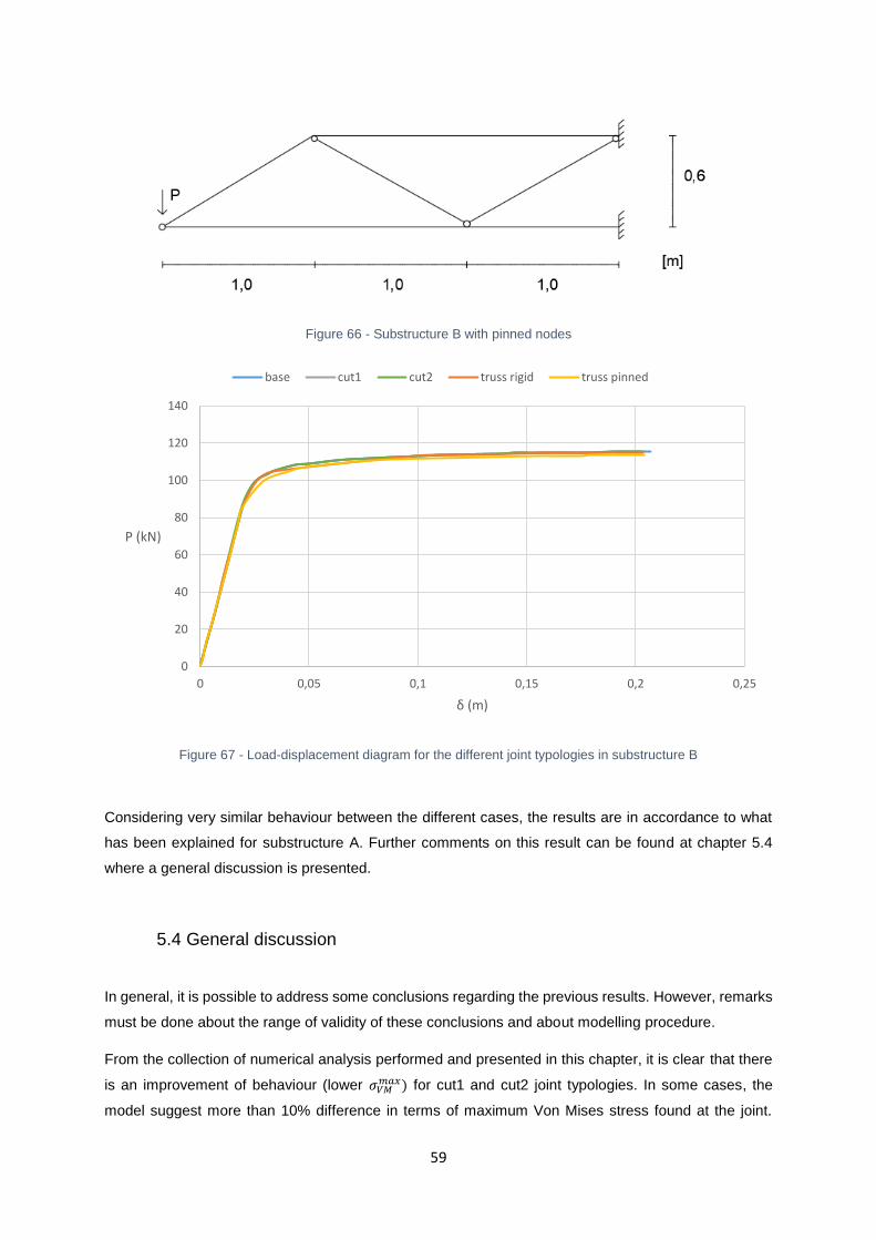
59

Figure 66 - Substructure B with pinned nodes

Figure 67 - Load-displacement diagram for the different joint typologies in substructure B

Considering very similar behaviour between the different cases, the results are in accordance to what

has been explained for substructure A. Further comments on this result can be found at chapter 5.4

where a general discussion is presented.

5.4 General discussion

In general, it is possible to address some conclusions regarding the previous results. However, remarks

must be done about the range of validity of these conclusions and about modelling procedure.

From the collection of numerical analysis performed and presented in this chapter, it is clear that there

is an improvement of behaviour (lower 𝜎𝑉𝑀𝑚𝑎𝑥) for cut1 and cut2 joint typologies. In some cases, the

model suggest more than 10% difference in terms of maximum Von Mises stress found at the joint.

0

20

40

60

80

100

120

140

0 0,05 0,1 0,15 0,2 0,25

P (kN)

δ (m)

base cut1 cut2 truss rigid truss pinned

60

These results have showed to be more expressive with higher loads and when the section is more

stressed.

In general, this improvement of behaviour could be explained by the presence of material inside the

chord that is working as a “stiffener” allowing for lower values of deformation and for redistribution of the

stresses to the other face of the chord.

For substructure A the results suggest that the hole in Cut1 is contributing to increase the stress

distribution on the face of the chord, and can be problematic if the bracing element that is prolonged is

too large. The presence of the hole may origin also problems of other nature like accumulation of waste,

if not closed. The choice of which element to prolong should take into account the size of the consequent

hole and which is the most stressed element.

Global rigidity of the structure is not changed with the different joint typologies and its behaviour is in

accordance with the structure with pinned and rigid nodes, which also indicates that the modelling

procedure of the detailed connections is accurate enough to describe the global behaviour of the

structure.

A comment about the global rigidity results should be done. These type of structures are subjected

mainly to axial forces, not only because the loads are applied at the nodes but also due to the relative

rigidity between brace and chord members. With this is mind, it makes sense that modelling with rigid

and pinned nodes in these conditions do not show great difference. The same is true for the

substructures modelled with the detailed joint typologies (models T+S). In fact, this is in accordance to

what is suggested in Eurocode [8] and CIDECT [33] that these kind of structures can be modelled with

a reasonable level of safety considering pinned nodes.

On the other hand, in the case of truss girders, if the members are subjected mainly to axial force, and

for this geometry, prolongation of the members in this direction will not change much the global rigidity

of the structure.

The range of validity of the results is within the scope of the geometrical, material, loading and boundary

conditions characteristics of the structure and modelling procedure. Further experimental tests are part

of the work package for which IST is responsible and will serve as a great validation of these results for

these conditions, allowing for the calibration of the models and for a better understanding of the

technology impact. One of the main goals is to give enough information about the behaviour of the

substructures so that experimental tests can be prepared and it is only with the collection of results from

numerical and experimental campaign (for both the substructures and truss girder) that further

conclusions can be made with more reliability.

61

6. Parametric analysis

After the collection of results presented in last chapter, it is interesting to perform a sensibility analysis

on some parameters that characterize the behaviour of the connection itself. The scope of the

parametric analysis is to investigate the effect of the thickness of the bracing and chord members on

the comparison results of the joint typologies using laser cut technology.

To be coherent with previous analysis the evaluation of the behaviour will be presented, again, in the

form of maximum Von Mises stress ( 𝜎𝑉𝑀𝑚𝑎𝑥) found at the joint.

Based on Vallourec design catalogue (the partner responsible for producing the profiles) the numerical

models were performed with the following thicknesses

For the bracings tb = {3.2 ; 4 ; 5 ; 6.3} (mm)

For the chord tc ={4 ; 5 ; 6.3 ; 8 ; 10} (mm)

The parametric analysis is divided in two parts. In the first part, the thickness of the chord profile is fixed

(in its original design value) and the thickness of the brace members (tb) is changed. In the second part,

the thickness of the brace profile is fixed (in its original design value) and the chord thickness (tc) is

iterated. Brace and chord thickness representation are clear in Figure 69.

The analysis is done for base, cut1 and cut2 for every thickness and the comparison of the last two is

done with the first in terms of percentage reduction of the 𝜎𝑉𝑀𝑚𝑎𝑥 at the connection level. The comparison

is done between joint typologies (Table 21 and Table 22).

The node chosen for this sensibility analysis was node NA-2 (Figure 68), because it was one of the

nodes that showed the best results in the previous analysis and due to its location in the truss girder, it

is the one considered to be of interest to explore the feasibility of the technology.

Figure 68 - Node of interest used in the sensibility analysis

The load (P=100kN) and boundary conditions are the same for every case. For a correct parametric

study, only the thickness of the shell elements (corresponding to the node that is being studied) is

62

changed. Otherwise, if the thickness of the linear elements (beam elements corresponding to the rest

of the truss girder) were also changed, the distribution of stresses in the structure would change and the

boundary conditions for the joint would not be the same.

Later on, the parametric analysis suggest a clear trend on the sensibility of joint behaviour to chord

thickness and an improvement of results when using LCT technology is analysed for this case in more

detail, in terms of loadings vs local displacement.

Figure 69 - Brace and chord thickness representation

6.1 Parametric analysis of the bracing thickness

The results are presented in Table 21, in which, for each value of the thickness of the brace it is showed

the value of 𝜎𝑉𝑀𝑚𝑎𝑥 for the different joint typologies and respective differences to the base case.

Table 21 - Results on the joint typologies behaviour by varying brace thickness


tb base cut1 dif to base cut2 dif to base

[mm] [MPa] [MPa] [%] [MPa] [%]

3,2 437 395 -9,6 402 -8,0

4 428 381 -11,0 397 -7,2

5 414 367 -11,4 385 -7,0

6,3 395 361 -8,6 370 -6,3

7,1 383 361 -5,7 366 -4,4

63

From the results, it is possible to draw the sensibility of each joint typology behaviour when increasing

the brace thickness (Figure 70). The blue line represents the difference (in percentage) of cut1 to base

type for the different values of thicknesses. The orange line represents the same but with respect to

cut2 and base type difference.

Figure 70 - Evolution of the difference in terms of 𝜎𝑉𝑀𝑚𝑎𝑥 from cut1 and cut2 to base case when increasing brace

thickness

The best results on cut1 (in comparison with cut2) can be explained by the fact that this σVMmax is located

on the vertical bracing, which in this typology is extended at its full cross section (hence improving the

results more than it would on cut2 in which only half of the cross section is prolonged)

For lower values of thickness the concentration of stress on this sections (due to the fact that is too thin),

do not allow for greater conclusions about the differences in joint typologies.

On the other hand, for greater values of bracing thickness the location of the maximum stress is shifting

to the chord, and so a change in the thickness of the braces (alone) would have a reduced impact on

the comparison the joint typologies, hence the reduction in the difference for both joint typologies.

The best result (in terms of improvement when compared to base typology) seems to be on the

intermediate values of thicknesses, in which the bracing is not thin enough to concentrate the stress on

its member and it’s not thick enough so that the maximum stress is shifted to the chord.

0,0

2,0

4,0

6,0

8,0

10,0

12,0

14,0

2 3 4 5 6 7 8

Δ (%)

brace thickness (mm)

dif cut1 dif cut2

64

6.2 Parametric analysis of the chord thickness

The same procedure is applied for the evaluation of the sensitivity to the chord thickness, and the results

are presented in Table 22.

Table 22 - Results on the joint typologies behaviour by varying chord thickness


tc base cut1 dif cut1 cut2 dif cut2

[mm] [MPa] [MPa] [%] [MPa] [%]

4 561 461 -17,8 474 -15,5

5 496 419 -15,5 427 -13,9

6,3 437 395 -9,6 402 -8,0

7,1 410 395 -3,7 396 -3,4

8 398 395 -0,8 396 -0,5

10 396 395 -0,3 395 -0,3

Following the same reasoning, the evolution of the different joint typologies for the different thicknesses

show a clearer trend in Figure 71.

Figure 71 - Evolution of the difference in terms of 𝜎𝑉𝑀𝑚𝑎𝑥from cut1 and cut2 to base case when increasing chord

thickness

0,0

2,0

4,0

6,0

8,0

10,0

12,0

14,0

16,0

18,0

20,0

3 4 5 6 7 8 9 10 11

Δ (%)

chord thickness (mm)

dif cut1 dif cut2

65

In fact, the results show a clear trend when increasing the thickness of the chord member. For greater

values of thickness the difference between the joint typologies decrease, suggesting that the joint

typologies taking advantage of laser cut technology (cut1 and cut2) lose their differential factors. On the

contrary, for decreasing thicknesses the advantage of using cut1 and cut2 are clear

The explanation could lie within the failure mode and the increase in rigidity due to the presence of

material inside the chord.

For this type of connection and geometry, the failure mechanism suggested by Eurocode is the chord

face failure, in which the face of the chord is deformed excessively. The results suggest that an

advantage of the joint typologies using LCT is that there is material inside the chord that can help

preventing this type of failure. In fact, this is in line with the results, since the thicker the chord section is

the less prone is the face to get deformed.

Moreover, with increasing thickness, the location of the max stress is in the bracing elements, and so

an increase of the thickness of the chord would not have a great impact on this value.

To explore this idea, attention was given to the local behaviour of the connection for lower values of

thickness of the chord (Chapter 6.3).

6.3 Local behaviour

The results from the previous parametric analysis suggest a high sensibility to deformation for lower

values of thickness of the chord and improvements in the joint behaviour when using Laser Cut

Technology in the joint typologies for these cases.

The 𝜎𝑉𝑀𝑚𝑎𝑥 parameter was evaluated and to confirm this suggestion a simple study of the local behaviour

is performed. In fact, the local behaviour of the different joint typology for brace thickness equal to 4mm

is shown and it is clear on the deformed configuration the effects of the prolongation of the profiles ( the

figures are under an amplification factor of 3 so that the representations are explicit).

Figure 72 - Deformation of base type for tb=4mm

66

For the base joint typology (Figure 72), it is clear the deformation on the face of the chord both at the

intersection with the vertical bracing and with the diagonal one.

Figure 73 - Deformation of cut1 type for tb=4mm

On the contrary, for the case of cut1 (Figure 73), in which there is the prolongation of the vertical element

into the lower face, the deformation is lower at the intersection between the chord and this vertical

element. In this case, the diagonal profile stops and it is welded on the face, so it is expected (as in base

case) to happen some deformation at this location.

Figure 74 - Deformation of cut2 type for tb=4mm

In the case of Cut2 (Figure 74), the deformed configuration shows the lowest values of deformation at

the chord upper face level. This is highly suggestive of what has been presented in the beginning of this

chapter, and it indicates that it is due to the prolongation (even though it is only at half of the original

cross sections profile) of the bracings into the chord.

67

To explore this, a simple comparative local behaviour study of the different joint typologies for different

thickness was performed, considering the displacement (in the plane of the loading – y) of the face of

the chord. This out of plane displacement (with respect to the face of the chord) was plotted against the

increasing load in the substructure.

To maintain a coherent analysis this was done in the same conditions as the numerical study, and in

the same node of interest of the parametric analysis.

Due to the deformed configuration, two locations were evaluated, nj-1 and nj-2, respectively at the

interface between the vertical bracing and the chord and between the diagonal bracing and chord, as

represented in the Figure 75.

Figure 75 - Representation of Nj-1 and Nj-2 for the local study

The numerical model was analysed for the set of chord thicknesses considered relevant for the type of

analysis, tc = {3; 4 ; 5} (mm), while the thickness of the bracing was maintained constant for the different

models, tb = {3.2} (mm)

68

Figure 76 - Load-displacement curve for Nj-1 (tc=3mm)



0

20

40

60

80

100

120

0 0,005 0,01 0,015 0,02 0,025 0,03

P (kN)

displacement (m)

base cut1 cut2

0

20

40

60

80

100

120

0 0,005 0,01 0,015 0,02 0,025 0,03

P (kN)

displacement (m)

base cut1 cut2

0

20

40

60

80

100

120

0 0,005 0,01 0,015 0,02 0,025 0,03

P (kN)

displacement (m)

base cut1 cut2

69




0

20

40

60

80

100

120

0 0,005 0,01 0,015 0,02 0,025 0,03 0,035

P (kN)

displacement (m)

base cut1 cut2

0

20

40

60

80

100

120

0 0,005 0,01 0,015 0,02 0,025 0,03 0,035

P (kN)

displacement (m)

base cut1 cut2

0

20

40

60

80

100

120

0 0,005 0,01 0,015 0,02 0,025 0,03 0,035

P (kN)

displacement (m)

base cut1 cut2

70

These results are in line with the previous ones and confirm the parametric analysis. The plots suggest

that the presence of material inside the chord affect the local behaviour, i.e., joint typologies that are

characterized by the prolongation of elements have showed to behave better and have lower values of

displacement at key locations (nj-1 and nj-2), for lower values of thicknesses of the chord. With

increasing thickness, the behaviour tends to be similar.

For lower values of thickness, tb=3mm, it is interesting to notice the similar behaviour between joint

typologies. At nj-1(Figures 76-78), the behaviour is similar between cut1 and cut2, while at nj-2 (Figures

79-81) base and cut1 are the ones showing load-displacement curves alike. In this last case, the

extension is done in the vertical element, and nj-2 is located at the diagonal one, so practically no effect

on the displacement is expected at this location.

This behaviour suggest that prolonging half of its original cross section (cut2) could be enough to

achieve practically the same results as prolonging the element in its whole cross section (cut1).

Due to these results, future studies should include testing structures in which the governing mechanism

of the truss girder is the collapse of the joint and, in particular, the chord face failure to which the results

indicate the improvement of behaviour when using laser cut technology.

Results suggest, for the same thickness, an increase in rigidity for joint typologies using LCT.

Considering this, one can look for similar behaviour by comparing base type joints with LCT joints with

lower thickness of the chord (Figure 82-85)

Figure 82 shows this clearly, by comparing load-displacement curves of cut1 and base cases with

different thicknesses, at nj-1 location. In this case, base (t=4mm) and cut1 (t=3mm) show similar

behaviour. The same is true for base (t=5mm) and cut1 (t=4mm). It can be noted that there is a limit for

this and for the exemplificative case of t=2.5mm the rigidity is lower with respect to base case. For cut2

case at nj-1, similar results can be found and are shown in figure 83.

At nj-2, same conclusions can be withdrawn and Figure 85 shows that base type joints with 4mm of

thickness of the chord can have similar behaviour to cut2 with only 3mm.

This suggest that it is possible to have the same behaviour of traditional joints but with lower values of

thickness of the chord if laser cut technology is used.

71

Figure 82 - Load-displacement curve for base and cut1 cases at nj-1


0

20

40

60

80

100

120

0 0,005 0,01 0,015 0,02 0,025 0,03

P (kN)

displacement (m)

cut1 t=2.5mm cut1 t=3mm cut1 t=4mm base t =4mm base t =5mm

0

20

40

60

80

100

120

0 0,005 0,01 0,015 0,02 0,025 0,03

P (kN)

displacement (m)

cut2 t=2.5mm cut2 t=3mm cut2 t =4mm base t=4mm base t=5mm

72


Figure 85 - Load-displacement curve for base and cut2 at nj-2

0

20

40

60

80

100

120

0 0,005 0,01 0,015 0,02 0,025 0,03 0,035 0,04 0,045

P (kN)

displacement (m)

cut1 t=2.5mm cut1 t=3mm cut1 t=4mm base t=3mm base t=4mm

0

20

40

60

80

100

120

0 0,005 0,01 0,015 0,02 0,025 0,03 0,035 0,04 0,045

P (kN)

displacement (m)

cut2 t=2.5mm cut2 t=3mm cut2 t=4mm base t=3mm base t=4mm

73

7. Conclusions and Future Studies

7.1 Conclusions

General conclusions about the results were highlighted throughout this dissertation but a collection of

these, remarks about the modelling and future studies are included in this final chapter.

The different bracing elements at the connections were modelled by overlapping the members in such

a way that the degrees of freedom of elements in the same space location are the same. In this way,

full rigidity between the members is assumed and the researcher / engineer should have a critical view

about the behaviour in terms of stress distribution and plastic strain.

Abaqus allows modelling a more realistic interaction between the section members in a way that the

contact relationship is inputted and interaction properties for normal and shear resistance are given to

the software. This was not the type of modelling procedure used in numerical models in this work but it

can be used for a more precise analysis and for studying different failure modes. Further experimental

results can be used to calibrate these parameters and for a more complete numerical model of the joints

configurations using Laser Cut Technology. In fact, the modelling procedure will be evaluated during the

experimental campaign, when the results from the testing will be compared with the numerical models.

Hence, only after the laboratory work package further conclusions about the modelling can be drawn.

The fact that the square hollow sections were modelled as perfect squares and without round angles in

the corners is an assumption that can be done [47,72] but in certain cases it may lead to unrealistic

results due to the concentration of stresses that can arise at this location in the numerical model.

Comparing all joint typologies, cut1 and cut2 show an improvement of behaviour in terms of 𝜎𝑉𝑀𝑚𝑎𝑥 at the

connection level. In some cases, a reduction over 10% was calculated when using these alternatives.

This positive results were achieved when the section was more stressed (higher loads) and only in the

case of substructure A. This can be indicative of different benefits of the use of this technology in different

situations and only increase the need for more numerical models and for execution of the experimental

program already planned.

A more uniform stress distribution at the joint is possible due to the extension of the bracing element. In

fact, higher stresses at the outer face of the chord due to the extension of the bracing are compensated

by the reduction at the inner face.

In cases of members with different cross sections concentrating at the nodes, the issue of which member

to extend was mentioned. Preliminary results from the numerical model indicate that the size of the

element has an impact on the distribution of stresses and in the specific conditions of the structure and

of the modelling procedure, the prolongation of the smaller one has showed to be an advantage.

Possible explanations for this can be the size of the consequent hole produced by the elongation of the

profile that weaken the joints, but further investigation on this topic is required.

74

Results from the numerical analysis of the different joint typologies have not shown differences in terms

of global rigidity of the structure for higher values of chord thickness, which indicate that structures of

this type can still be modelled with hinged nodes. This is considered to be, also, an indication of a good

modelling procedure for models combining linear and planar elements (model T+J). However, this was

done considering the initial design of the substructures. Later, the rigidity issue proved to be more

sensitive for lower values of thickness of the chord at a local level, which could also affect the global

behaviour.

Similar results between cut1 and cut2 also suggest prolongation only half of the cross section is enough

to achieve the positive results in terms of improvement of structural behaviour. The advantage is that in

this last case only a slot is opened at the chord face and no hole is needed, which can be even more

problematic in the case of bigger bracing profiles. On the other hand, the cutting of the profile in this

shape could be slightly more complicated. In addition, due to its innovative design, this solution would

require more studies in terms of local behaviour of the cross section. In particular for cut2, in case of

elements in compression further studies on the possibility of local buckling of the extended profiles

should be performed due to its modified cross sections.

Subsequent parametric analysis tried to evaluate this performance when varying chord and brace

thickness. Results suggest a higher rate of improvement between joint typologies for lower values of

chord thickness and that the material inside the chord (for cut1 and cut2 solutions) has an impact on the

deformation of the chord face. In general, prolongation of only half of the cross sections (cut2) appears

to be enough to contribute to this structural behaviour improvement.

The preliminary design of the substructures indicate that the IST Civil Engineering Laboratory have at

the moment capacity to test this structures until failure and monitor its behaviour during loading.

Considering the increase in the rigidity of the joints by using Laser Cut technology in comparison with

the traditional method (comparison with base case), it is possible to maintain the same structural

behaviour for lower values of thickness of the chord. This suggest that it is possible to design lighter

structures, more economical and aesthetical appealing, with the same level of performance. However,

the changes in the joint design could modify the design procedure of the overall truss.

7.2 Future Studies

The author recommendation is that experimental work package include cut1 and cut2 joint typologies in

the nodes of interest used for the numerical analysis and with the same geometry and conditions that

were used in the design. In order to explore the potential of the technology, and considering the results

of the parametric analysis, the author also suggest that future studies should consider a reduction of

the thickness of the chord to what has been used in the preliminary design.

One of the advantages of the technology for column-beam connections that is well documented [7] is

the fact the interlocking of the profiles (through openings or slots in one another by laser cut) allows for

75

a safer structural behaviour in case of breakage of the welds. In this sense, future modelling of this

technology should study the effects of welds, so that conclusions about behaviour posteriori to weld

failure can be extended to truss girders applications. Following this indication, colleague’s researchers

at IST and participating in this project are already including welds in their numerical models.

Extendibility of the work presented in this dissertation to other cross sections (Rectangular and Circular

Hollow Sections and open sections) is of paramount importance for greater conclusions about the

technology, and its study has already started by other colleagues in the project.

In addition, for a more complete generalization of the conclusions for the extendibility of the technology

for truss girder applications, other type of truss girder designs should be considered. The author suggest

the study of laser cut joint typologies in Vierendeel type trusses (where the members form rectangular

openings), in which bending forces are more significant and in which the technology could play a more

important role in the rigidity of the structure and its connections.

One of the possible application of the technology is the optimization of gusset plates for the connection

of hollow section profiles and the insertion of them inside the chord trough precise laser cutted holes.

Further studies (both numerical and experimental) analysis are needed to test this innovative solution

with intermediate plate.

For base, cut1 and cut2, the cross section at the end of the profile will be modified in terms of geometry,

it will be cutted in a direction that is parallel to the chord face (and not cutted perpendicular to the mean

axis) for the correct welding to the chord. This modification of the cross section at the connection level

is out of the scope of today’s Eurocode design formulae. Moreover, the consideration of material inside

chord section is not foreseen in today’s regulation. This only contributes to the importance of building a

set of rules and for an appropriate and specific design approach to a complete new and innovative

technology.

In fact, in case of positive results, LASTEICON work package includes the creation of design guidelines,

which aim at constituting an alternative for designers and engineers to use laser cut steelwork solutions

in their projects with a reliable degree of safety.

77

References

[1] “Research Fund for Coal and Steel.” [Online]. Available:

http://ec.europa.eu/research/industrial_technologies/rfcs_en.html.

[2] European Comission, “Action Plan for a competitive and sustainable steel industry in Europe,”

2013.

[3] ECORYS SCS Group, “FWC Sector Competitiveness Studies N° B1/ENTR/06/054 –

Sustainable Competitiveness of the Construction Sector.”

[4] S. Morino and K. Tsuda, “Design and Construction of Concrete-Filled Steel Tube Column

System in Japan,” Earthq. Eng. Eng. Seismol., vol. 4, no. 1, pp. 51–73, 2003.

[5] S. P. Schneider and Y. . Alostaz, “Experimental behavior of connections to concrete filled steel

tubes,” J. Constr. Steel Res., vol. 40, no. 2, pp. 95–127, 1998.

[6] C. Castiglioni, “LASTEICON EU Research Proposal.” 2015.

[7] L. CAMPOLUNGHI, “I beams to CHS column connection an innovative typology - Master

thesis,” Politecnico di Milano, 2012.

[8] European Committee for Standardization (CEN), EN 1993-1-8, Eurocode 3 – Design of steel

structures – Part 1-8: Design of joints, vol. 3. 2005.

[9] “Euro-build in steel: evaluation of client demand, sustainability and future regulations on the

next generation of building design in steel, CEC 7210-PR/381.”

[10] “Slefty.” [Online]. Available: http://slefty.com/the-future-of-steel-products/.

[11] D. B. Ed. Moore and F. Wald, Design of Structural Connections to Eurocode 3 - Frequently

Asked questions. Watford: Publishing House of Czech Technical University in Prague, 2003.

[12] X. L. Zhao and L. W. Tong, “New development in steel tubular joints,” Adv. Struct. Eng., vol.

14, no. 4, pp. 699–715, 2011.

[13] E. Bortolotti et al., “Testing and modelling of welded joints between elliptical hollow sections,

Proceedings of 10th International Symposium on Tubular Structures,” 2003, pp. 259–264.

[14] C. Pietrapertosa and J. P. Jaspart, “Study of the behaviour of welded joints composed of

elliptical hollow sections”, Proceedings of the 10th International Symposium on Tubular

Structures,” 2003, pp. 601–608.

[15] Y. S. Choo, J. X. Liang, and L. V. Lim, “Static strength of elliptical hollow section X-joint under

brace compression, Proceedings of the 10th International Symposium on Tubular Structures,”

2003, pp. 253–258.

78

[16] C. Matsui, “Strength and behaviour of frames with concrete filled square steel tubular columns

under earthquake loading,” in 1st International Speciality Conference on Concrete Filled Steel

Tubular Structures, 1985, pp. 104–111.

[17] J. Kawaguchi, S. Morino, and T. Sugimoto, “Elasto-plastic behaviour of concrete-filled steel

tubular frames,” in Composite construction in steel and concrete III, 1997, pp. 272–281.

[18] K. C. Tsai, J. W. Lai, C. H. Chen, B. C. Hsiao, Y. T. Weng, and M. L. Lin, “Pseudo Dynamic

Tests of a Full Scale CFT/BRB Composite Frame,” in Structures 2004: Building on the Past,

Securing the Future, 2004, pp. 1–10.

[19] H. Yang, D. Lam, and L. Gardner, “Testing and analysis of concrete-filled elliptical hollow

sections, Engineering Structures,” vol. 30, no. 12, pp. 3771–3781, 2008.

[20] X. L. Zhao and J. A. Packer, “Tests and design of concrete-filled elliptical hollow section stub

columns,” Thin-Walled Struct., vol. 47, no. 6–7, pp. 617–628, 2009.

[21] A. D. Christitsas, D. T. Pachoumis, C. N. Kalfas, and E. G. Galoussis, “FEM analysis of

conventional and square bird-beak SHS joint subject to in-plane bending moment -

experimental study,” J. Constr. Steel Res., vol. 63, no. 10, pp. 1361–1372, 2007.

[22] BLM Group, “Inspired for Tube,” No.9, 2008.

[23] R. Aloke, V. Girish, R. F. Scrutton, and P. A. Molian, “A model for prediction of dimensional

tolerances of laser cut holes in mild steel thin plates,” Int. J. Mach. Tools Manuf., vol. 37, no. 8,

pp. 1069–1078, 1997.

[24] M. Harničárová, J. Zajac, and A. Stoić, “Comparison of different material cutting technologies in

terms of their impact on the quality of structural steel,” Teh. Vjesn., vol. 17, no. 3, pp. 371–376,

2010.

[25] M. C. Bittencourt, L. R. O. De Lima, P. C. G. S. Vellasco, J. G. S. Silva, and L. F. C. Neves, “A

Numerical Analysis of Tubular Joints under Static Loading,” Proc. APCOM’07 conjunction with

EPMESC XI, pp. 3–6, 2007.

[26] M. L. Santos, L. R. O. De Lima, and A. M. S. Freitas, “Modelagem numérica de ligações K,” in

Métodos Numéricos em Engenharia, 2011.

[27] B. E. Gorenc, R. Tinyou, and A. A. Syam, Steel Designer’s Handbook. Sydney: UNSW Press,

2005.

[28] A. M. C. ARAÚJO, “Estudo do comportamento de ligações metálicas entre perfis tubulares e

chapas de gousset. Tese de Mestrado,” Faculdade de Engenharia da Universidade do Porto,

2012.

[29] Tata Steel & BCSA, “Cost supplement, Steel construction,” 2013.

[30] Research Fund for Coal and Steel Unit, “Economics of steel-framed buildings in Europe

79

(ESE),” 2012.

[31] ECCS\CECM\EKS, “Statistical report 2004, European Convention for Constructional

Steelwork,” 2004.

[32] CIDECT The International Committee for Research and Technical Support for Hollow Section

Structures, “http://www.cidect.org/.” .

[33] J. A. Packer, J. Wardenier, X.-L. Zhao, G. J. van der Vegte, and Y. Kurobane, CIDECT -

Design Guide 3 for rectangular hollow section (RHS) joints under predominantly static loading.

2009.

[34] A. Maria, S. Freitas, and G. V. Nunes, “Overview of Tubular Joints - EC3 X New CIDECT

formulations,” in Connections VII - 7th International Workshop on Connections in Steel

Structures, 2012, no. 1, pp. 1–10.

[35] L. H. Lu, G. D. de Winkel, Y. Yu, and J. Wardenier, “Deformation Limit for the Ultimate Strength

of Hollow Section Joints,” in International Symposium on Tubular Structures, 1994, pp. 341–

347.

[36] Y. S. Choo, X. D. Qian, J. Y. R. Liew, and J. Wardenier, “Static strength of thick-walled CHS X-

joints — Part I . New approach in strength definition,” vol. 59, pp. 1201–1228, 2003.

[37] International Institute of Welding (IIW), Design recommendation for hollow section joints—

Predominantly statically loaded. 1989.

[38] I. S. Mayor, G. V. Nunes, and A. M. S. Freitas, “Theoretical and experimental analysis of

RHS/CHS K gap joints,” vol. 66, no. 3, pp. 295–300, 2013.

[39] M. Costa-Neves;Lima;Vellasco;Silva, “Resistance and elastic stiffness of RHS ‘ T ’ joints : part I

- axial brace loading,” vol. 3, no. Figure 1, pp. 2159–2179, 2015.

[40] M. Johansson and T. Löfberg, “Modelling of pitched truss beam with Finite Element method.

Considering response of second order effects and imperfections. Master of Science Thesis,”

Chalmers University of Technology, 2011.

[41] M. Abambres and M. R. Arruda, “Finite element analysis of steel structures - A review of useful

guidelines,” Int. J. Struct. Integr., vol. 7, no. 4, pp. 490–515, 2016.

[42] M. A. Serrano-López, C. López-Colina, J. J. Del Coz-Díaz, and F. L. Gayarre, “Static behavior

of compressed braces in RHS K-joints of hot-dip galvanized trusses,” J. Constr. Steel Res., vol.

89, pp. 307–316, 2013.

[43] G. J. Van Der Vegte, “The influence of boundary conditons on the chord load effect for CHS

gap K-joints,” no. 2, pp. 433–444, 2004.

[44] L. Gardner and T. M. Chan, “Cross-section classification of elliptical hollow sections,” Steel

Compos. Struct., vol. 7, no. 3, p. 85, 2007.

80

[45] K. Mitsui, A. Satob, M. Latourc, V. Pilusoc, and G. ; Rizzanoc, “Experimental analysis and FE

modelling of square hollow sections under combined axial and bending loads,” ce/papers, vol.

1, no. 2–3, pp. 4732–4739, 2017.

[46] M. M. K. Lee, “Strength , stress and fracture analyses of offshore tubular joints using finite

elements,” vol. 51, pp. 265–286, 1999.

[47] I. Radić, D. Markulak, and M. Mikolin, “Design and FEM Modelling of Steel Truss Girder

Joints,” vol. 52, no. 2, pp. 125–135, 2010.

[48] M. Sa, “The effect of joint eccentricity on the distribution of forces in RHS lattice girders The

eff,” J. Constr. Steel Res., vol. 47, no. 3, pp. 211–221, 1998.

[49] L. M. Connelly and N. Zettlemoyer, “Frame Behaviour Effects on Tubular Joint Capacity,” in

International Symposium on Tubular Structures, 1989, pp. 81–89.

[50] H. M. Bolt, H. Seyed-Kebari, and J. K. Ward, “The Influence of Chord Length and Boundary

Conditions on K-Joint Capacity,” in 2nd International Offshore and Polar Engineering

Conference, 1992, pp. 347–354.

[51] B. E. Healy, “A Numerical Investigation into the Capacity of Overlapped Circular K-joints,” in

6th International Symposium on Tubular Structures, 1994, pp. 563–571.

[52] E. M. Dexter, M. M. K. Lee, and M. G. Kirkwood, “Effect of Overlap on Strength of K-joints in

CHS Tubular Members,” in International Symposium on Tubular Structures, 1994, pp. 581–

588.

[53] O. H. Bjornoy, “Static Strength of Tubular Joints, Phase II, Analyses and Tests of Gap and

Overlap K-Joints. Veritec Report No 91-3393, AS Veritec,” 1991.

[54] D. K. Liu, Y. Yu, and J. Wardenier, “Effect of Boundary Conditions and Chord Preload on the

Strength of RHS Uniplanar Gap K-Joints,” in 8th International Symposium on Tubular

Structures, 1998, pp. 223–230.

[55] D. K. Liu, Y. Yu, and J. Wardenier, “Effect of Boundary Conditions and Chord Preload on the

Strength of RHS Multiplanar Gap K-Joints,” in 8th International Symposium on Tubular

Structures, 1998, pp. 231–238.

[56] A. Jurčíkováa and M. Rosmanit, “FEM model of joint consisting RHS and HEA profiles,”

Procedia Eng., vol. 40, pp. 183–188, 2012.

[57] S. T. Lie, Z. M. Yang, S. P. Chiew, and C. K. Lee, “The ultimate behaviour of cracked square

hollow section T-joints,” ISSN, vol. 3, no. 1, pp. 443–458, 2007.

[58] G. Van Der Vegte, C. De Koning, R. Puthli, and J. Wardenier, “Numerical simulation of

experiments on multiplanar steel X-joints,” Int. J. Offshore Polar Eng., vol. 39, no. 4, pp. 55–67,

1991.

81

[59] M. Lee and S. R. Wilmshurst, “Numerical modelling of CHS joints with multiplanar double-K

configuration,” J. Constr. Steel Res., vol. 32, pp. 281–301, 1995.

[60] H. F. Chang, J. W. Xia, H. Chang, and F. J. Zhang, “Analysis on the Chord Side Wall Failure of

RHS T-Joints with Axial Compression Branch,” Adv. Mater. Res., vol. 163–167, pp. 323–326,

2011.

[61] L. G. Vigh and L. Dunai, “Finite element modeling and analysis of bolted joints of 3D tubular

structures,” Comput. Struct., vol. 82, no. 23–26, pp. 2173–2187, 2004.

[62] K. Wang, F. Shao, J. Xing, and X. Lü, “Research on hysteretic behavior of steel circular-tube

members under constant compression and cyclic bending,” J. Build. Struct., vol. 31, no. 1, pp.

35–38, 2010.

[63] Dassault Systèmes, ABAQUS 6.14 - ABAQUS/CAE User’s guide. 2014.

[64] L. Cannizzaro, E. Lo Valvo, F. Micari, and R. Riccobono, “H and P Mesh Refinement in the

Metal-Forming F.E.M. Analysis,” in Modelling of Metal Forming Processes, Dordrecht:

Springer, 1988, pp. 49–56.

[65] A. HyperWorks, Practical Aspects of Finite Element Simulation – A Student Guide, Altair

Engineering Inc. 2011.

[66] D. N. Veritas, “DNV-RP-C208 Determination of Structural Capacity by Non-linear FE analysis

Methods,” no. June. 2013.

[67] J. J. C. Díaz, M. A. S. López, C. L. Pérez, and F. P. Á. Rabanal, “Effect of the vent hole

geometry and welding on the static strength of galvanized RHS K-joints by FEM and DOE,”

Eng. Struct., vol. 41, pp. 218–233, 2012.

[68] A. Jurčíková and M. Rosmanit, “The Evaluation of Load-Bearing Capacity of the Planar CHS

Joint Using Finite Modeling,” vol. 7, no. 10, pp. 729–732, 2013.

[69] M. Tada and A. Suito, “Static and dynamic post-buckling behavior of truss structures,” vol. 20,

no. 97, pp. 384–389, 1998.

[70] European Committee for Standardization (CEN), 1993-1-5, Eurocode 3 — Design of steel

structures — Part 1-5: Plated structural elements. 2009.

[71] M. M. K. Lee, E. M. Dexter, and M. G. Kirkwood, “Strength of moment loaded tubular T/Y-joints

in offshore platforms,” Struct. Eng. J. Inst. Struct. Eng., vol. 73, no. 15, pp. 239–246, 1995.

[72] L. R. O. de Lima, L. F. da Costa-Neves, J. G. S. da Silva, and P. C. G. da S. Vellasco, “Análise

paramétrica de ligações ‘T’ com perfis tubulares em aço através de um modelo de elementos

finitos,” in XXVI Iberian Latin-America Congress on Computational Methods in Engineering,

2005.

Numerical Models on Innovative Steel Hollow Section Joints ...

Documents

Transcript of Numerical Models on Innovative Steel Hollow Section Joints ...