Numerical modeling of two-phase ﬂow in heterogeneous ... · PDF filepermeable media with...

Available online at www.sciencedirect.com

www.elsevier.com/locate/advwatres

Advances in Water Resources 31 (2008) 56–73

Numerical modeling of two-phase flow in heterogeneouspermeable media with different capillarity pressures

Hussein Hoteit a,1, Abbas Firoozabadi a,b,*

a Reservoir Engineering Research Institute, Palo Alto, CA, USAb Yale University, New Haven, CT, USA

Received 8 February 2007; received in revised form 15 June 2007; accepted 21 June 2007Available online 5 July 2007

Abstract

Contrast in capillary pressure of heterogeneous permeable media can have a significant effect on the flow path in two-phase immiscibleflow. Very little work has appeared on the subject of capillary heterogeneity despite the fact that in certain cases it may be as important aspermeability heterogeneity. The discontinuity in saturation as a result of capillary continuity, and in some cases capillary discontinuitymay arise from contrast in capillary pressure functions in heterogeneous permeable media leading to complications in numerical mod-eling. There are also other challenges for accurate numerical modeling due to distorted unstructured grids because of the grid orientationand numerical dispersion effects. Limited attempts have been made in the literature to assess the accuracy of fluid flow modeling in het-erogeneous permeable media with capillarity heterogeneity. The basic mixed finite element (MFE) framework is a superior method foraccurate flux calculation in heterogeneous media in comparison to the conventional finite difference and finite volume approaches. How-ever, a deficiency in the MFE from the direct use of fractional flow formulation has been recognized lately in application to flow in per-meable media with capillary heterogeneity. In this work, we propose a new consistent formulation in 3D in which the total velocity isexpressed in terms of the wetting-phase potential gradient and the capillary potential gradient. In our formulation, the coefficient of thewetting potential gradient is in terms of the total mobility which is smoother than the wetting mobility. We combine the MFE and dis-continuous Galerkin (DG) methods to solve the pressure equation and the saturation equation, respectively. Our numerical model isverified with 1D analytical solutions in homogeneous and heterogeneous media. We also present 2D examples to demonstrate the sig-nificance of capillary heterogeneity in flow, and a 3D example to demonstrate the negligible effect of distorted meshes on the numericalsolution in our proposed algorithm.� 2007 Elsevier Ltd. All rights reserved.

Keywords: Two-phase flow; Water injection; Heterogeneous media; Capillary pressure; Mixed finite element method; Discontinuous Galerkin; Slopelimiter

1. Introduction

Subsurface fluid flow problems are of importance inmany disciplines including hydrology and petroleum reser-voir engineering. In such flows, the process of displacementis mainly affected by the properties of the permeable med-ium, and fluids in single-phase both in homogeneous and in

0309-1708/$ - see front matter � 2007 Elsevier Ltd. All rights reserved.

doi:10.1016/j.advwatres.2007.06.006

* Corresponding author. Address: Yale University, New Haven, CT,USA.

E-mail address: [email protected] (A. Firoozabadi).1 Present address: ConocoPhillips Co., USA.

heterogeneous media. In two-phase immiscible flows, theinteractions between the permeable medium and the fluidsalso affect the path of flowing fluids. Such interactions aredefined by relative permeability and capillary pressure.While in a homogeneous medium, the effect of capillarypressure can be neglected, this may not be the case in het-erogeneous permeable media. The contrast in capillarypressure functions of different media may become a keyfactor in fluid flow. In single-phase flow and in two-phaseflow with negligible capillary pressure, fluids generallyflow through regions with high effective permeabilities. Inheterogeneous media with capillary pressure heterogeneity,

mailto:[email protected]

H. Hoteit, A. Firoozabadi / Advances in Water Resources 31 (2008) 56–73 57

capillary pressure forces may completely change the pathof the flowing fluids. In heterogeneous petroleum reser-voirs, depending on the recovery process, capillarity mayresult in improved recovery or poor recovery performance.In the imbibition process, capillarity may significantlyenhance the cross-flow in stratified reservoirs and thereforeimprove the recovery efficiency of oil from tight permeablemedia [1]. In the gravity drainage process, capillary forceshave an opposite effect resulting in low recovery efficiency[2,3]. A large body of literature is devoted to the modelingof two-phase flow in heterogeneous media without capillar-ity [4–9]. However, despite the fact that heterogeneity incapillary pressure may have a significant effect on flow,only a handful of authors have studied the problem. Yort-sos and Chang [10] studied analytically the capillary effectin steady-state flow in 1D heterogeneous media. Theyassumed a sharp but continuous transition of permeabilityto connect different permeable media of constant perme-abilities. Van Duijn and De Neef [11] provided a semi-ana-lytical solution for time-dependent countercurrent flow in1D heterogeneous media with one discontinuity in the per-meability, and studied the effect of the threshold capillarypressure on oil trapping. They introduced an interface con-dition to account for the entry pressure and saturation dis-continuity at the interface of different rock types. Niessneraet al. [12] and Reichenberger et al. [13] described the vanDuijn/De Neef interface condition in the context of a con-trol-volume finite element method (box-scheme). Beveridgeet al. [14] examined the sensitivity of the production rate tothe capillary forces. Correa and Firoozabadi [15] studiedthe effect of capillary heterogeneity on two-phase gas-oildrainage in 1D vertical flow. The authors demonstratedthat due to capillary pressure contrast, the gravity drainagemay become unstable. Without capillary pressure contrast,the drainage is always stable.

A large number of numerical methods have been devel-oped to model two-phase flow in heterogeneous media. Inthe commercial simulators for multiphase flow, the finitedifference (FD) and finite volume (FV) methods are thegeneral framework for numerical simulation for the studyof fluid flow in very large problems [16–18]. The conven-tional FD method, however, is strongly influenced by themesh quality and orientation, which makes the methodunattractive for unstructured gridding [19,20]. Recently,there have been attempts to improve the accuracy of theFD and cell-centered FV methods on unstructured grid-ding by using multi-point flux approximation techniques[21–25]. However, such techniques have not been demon-strated to be of value for heterogeneous media with con-trast in capillary pressure. The vertex-centered FV maybe superior to the cell-centered FV method [26–28]. How-ever, the former requires additional treatments to modelthe flow in control volumes containing different permeablemedia [29]. On the other hand, methods based on Galerkinfinite elements may not be robust in heterogeneous media.Helmig and Huber [30] compared three Galerkin-type dis-cretization methods. They showed that the standard and

the Petrov–Galerkin methods may produce unphysicalsolutions in heterogeneous media and severe mesh restric-tions are required for the stability of the fully upwindGalerkin method in multidimensional space.

Accurate approximation of the flow-lines and flux, andlow mesh dependency are desirable features for successfulnumerical schemes for modeling two-phase flow in hetero-geneous media. Such an accurate approximation can beachieved by the mixed finite element (MFE) method [31–33], which is superior to the control volume FE and Galer-kin FE methods in approximating the velocity field in het-erogeneous media [34,35]. Various authors have exploredthe MFE method for single-phase flow problems [36–40].Chavent et al. [41–43] extended the MFE method to two-phase flow with a single capillary pressure function byusing the fractional flow formulation, where the governingequations are written in terms of the total velocity and theglobal pressure. The global pressure is defined in terms ofthe arithmetic pressure of the wetting and non-wettingphases and an integral with the integrand containing frac-tional flow function and the derivative of the capillary pres-sure with respect to the wetting phase saturation. Thegradient of the global pressure was then evaluated to bea function of the fractional flow of the wetting phase,and the gradient of the capillary pressure. Such a formula-tion based on the fractional flow formulation is sound aslong as a single capillary pressure function is used for theentire permeable domain [42–46]. Since the MFE methodrequires the primary variable and its derivative (flux) tobe continuous at the gridblock interfaces, the fractural flowformulation with the global pressure as primary variablebecomes deficient for different capillary pressure functionsbecause of the discontinuity in global pressure at the inter-face [47] from saturation discontinuity. Nayagum et al. [48]used the average pressure instead of the global pressure tosolve the inconsistency problem. Their method is demon-strated only in 1D space. Other formulations have alsobeen used with the MFE method [49,50], but none of theproposed MFE formulations has been demonstrated fortwo-phase flow in multidimensional, heterogeneous mediawith different capillary pressure functions. In this work,we provide a MFE formulation in 2D and 3D heteroge-neous media that overcomes the drawbacks of the frac-tional flow formulation. Instead of the global pressurevariable that can be discontinuous in heterogeneous media,we use the wetting-phase pressure as a primary variablewhich is always continuous as long as none of the phasesis immobile. Our proposed formulation can correctlydescribe discontinuities in saturation due to different capil-lary pressure functions as well as discontinuities in capillarypressure at the interface of regions with threshold capillarypressures (that is, entry pressures).

In the conventional MFE method for elliptic and para-bolic equations, one calculates simultaneously the cell-pres-sures and the fluxes across the numerical block interfaces.The resulting linear system is relatively large and indefinite.In this work, we use the hybridized MFE method that

58 H. Hoteit, A. Firoozabadi / Advances in Water Resources 31 (2008) 56–73

provides a symmetric, positive definite linear system withthe face-pressures (traces of the pressure) as primaryunknowns. The hybridized MFE is algebraically equivalentto the conventional MFE but it is more efficient [33,37,51].

In addition to the flux calculation accuracy, anotherconcern is the approximation of the mobilities at the inter-face of the numerical blocks. First-order methods, such asthe conventional FD and FV methods, with a single-pointupstream weighting technique, may produce significantnumerical dispersion in the vicinity of sharp fronts in thesaturation [52,53]. Higher-order FD methods such asthe two-point upstream weighting, total variation dimin-ishing (TVD), and the essentially non-oscillatory (ENO)approaches [54–60] reduce the numerical dispersion. Instructured meshes in multidimensional space, these meth-ods can be implemented by using a directional splittingtechnique so that the 1D formulation can be applied ineach directional space [61]. Higher-order FV methods havebeen applied for different physical problems, such as con-servative laws, advection and Navier–Stokes equations,on unstructured meshes in 2D and 3D [62–67]. There are,however, few attempts in the literature to implementhigher-order FV methods for two-phase flow in heteroge-neous media on unstructured meshes in multidimensionalspace.

For our problem, the discontinuous Galerkin (DG)method is attractive because of its flexibility in describingunstructured domains by using higher-order approxima-tion functions. Its implementation is in line with saturationdiscontinuity. It also conserves mass locally at the elementlevel.

The DG method was first implemented for nonlinearscalar conservative laws by Chavent and Salzano [68],who found that a very restrictive time step is required tokeep the scheme stable. Chavent and Cockburn [69]improved the stability of the method by using a slope lim-iter following the work of van Leer [70]. Cockburn and Shuintroduced the Runge–Kutta Discontinuous Galerkin(RKDG) method [71,72], which is an extension of theDG method with higher-order temporal schemes. TheDG method has also been implemented for elliptic and par-abolic equations [73–76] and for incompressible two-phaseflow in porous media [77–80], where the method is used toapproximate both the pressure and saturation equations.In this work, however, we use the DG method with a sec-ond-order Runge–Kutta temporal scheme to approximateonly the saturation equation. The pressure equation isapproximated by the MFE method, as previously men-tioned. A multidimensional slope limiter [42] is used to pre-vent the DG scheme from developing spurious oscillationsin the saturation.

In the past, the MFE and DG methods have been usedfor different applications in single-phase [53,81–83] andtwo-phase flow with a single capillary pressure functionin heterogeneous media [43]. In this work, we advancethe applicability of the combined MFE-DG method in het-erogeneous media on unstructured gridding, where we

show how to account for the discontinuity in saturationfrom different capillary pressure functions. The centraltheme of this work is the displacement of the non-wettingphase by the wetting phase. In the displacement of a wet-ting phase by the a non-wetting phase, the issue of thethreshold capillary (entry) pressure rises. For the sake ofcompleteness, we include the numerical modeling of thethreshold capillary pressure in 1D in this work. In a futurework, we will present examples of its significance in multi-dimensional flow.

This paper is organized as follows. First, we review thegoverning equations of two-phase, incompressible fluidflow in porous media. We then propose a new formulationfor the MFE method and present the approximations ofthe velocity and volumetric balance equations. The DGmethod is then used for the saturation equation, wherewe approximate the saturation by using first-order polyno-mials on general elements. We also provide several numer-ical examples in one and multidimensional space inheterogeneous media.

2. Mathematical formulation

The flow of two incompressible and immiscible fluids inporous media is described by the saturation equation andthe Darcy law of the wetting and the non-wetting fluidphases. The saturation equation of phase a is given by:

/oSa

otþr � ðvaÞ ¼ F a; a ¼ n;w; ð1Þ

where / is the porosity of the medium, the subscripts n andw denote the non-wetting and wetting phases, respectively,Sa, F a, and va are the saturation, the external volumetricflow rate, and the volumetric velocity of phase a,respectively.

The velocity va is described by the Darcy law as follows:

va ¼ �kra

la

Kðrpa þ qagrzÞ; a ¼ n;w: ð2Þ

In Eq. (2), K is the absolute permeability tensor, pa, qa, kra,and la are the pressure, density, relative permeability, andviscosity of phase a, respectively, g is the gravity accelera-tion, and z is the depth. The saturations of the phases areconstrained by:

Sn þ Sw ¼ 1; ð3Þand the two pressures are related by the capillary pressure(pc) function:

pcðSwÞ ¼ pn � pw: ð4ÞAs previously mentioned, the fractional flow formulationused by several authors [42–46] becomes inconsistent whenimplemented in the MFE method because of the disconti-nuity of the global pressure in heterogeneous media. In thissection, we present a new formulation that avoids thedrawback of the fractional flow implementation. We definethe flow potential, Ua, of phase a as follows:


Ua ¼ pa þ qagz; a ¼ n;w: ð5ÞReplacing Eq. (5) in Eq. (4), we get the following expres-sion of the capillary potential, Uc [84]:

Uc ¼ Un � Uw ¼ pc þ ðqn � qwÞgz: ð6ÞThe total velocity vt is then written in terms of two velocityvariables va and vc, as follows:

vt ¼ vn þ vw ¼ �ktKrUw|fflfflfflfflfflfflffl{zfflfflfflfflfflfflffl}va

�knKrUc|fflfflfflfflfflfflffl{zfflfflfflfflfflfflffl}vc

¼ va þ vc: ð7Þ

In the above equation, ka = kra/la is the mobility of phasea. The velocity variable va has the same driving force as thewetting-phase velocity but with a smoother mobility kt,that is, kt = kn + kw, than the wetting phase mobility.

The wetting-phase velocity, in terms of va and the wet-ting-phase fractional function, fw = kw/kt, reads as:

vw ¼kw

kt

ð�ktKrUwÞ ¼ fwva: ð8Þ

The expression of the balance of both phases in terms of va

and vc can be obtained by adding the saturation equationsgiven in Eq. (1) and using Eqs. (3) and (7). The governingequations are, therefore, the total volumetric balance equa-tion and the saturation equation of the wetting phase ex-pressed in terms of va and fw from Eq. (8), that is,

r � ðva þ vcÞ ¼ Fn þ Fw; ð9Þ

/oSw

otþr � ðfwvaÞ ¼ Fw: ð10Þ

The system of Eqs. (9) and (10) are subject to appropriateinitial and boundary conditions to describe the initial satu-rations, boundary pressures, and external flow rates. LetC = CD [ CN be the boundary of the computational do-main X, where CD and CN are non-overlapping boundariescorresponding to Dirichlet and Neumann boundary condi-tions. The volumetric balance equation (9) is subject to thefollowing boundary conditions:

pwðor pnÞ ¼ pD on CD;

ðva þ vcÞ � n ¼ qN on CN;ð11Þ

and the saturation equation (10) is subject to:

Sw ¼ S0 in X;

Swðor SnÞ ¼ SN on CN;ð12Þ

where n denotes the outward unit normal, qN and pD arethe imposed volumetric injection rate and pressure at CN

and CD, respectively, S0 is the initial saturation, and SN

is the boundary saturation of the injected fluid at CN.

3. Approximation of the flux

We consider a spatial discretization of the domain Xconsisting of triangles or quadrilaterals in 2D, and tetrahe-drons, prisms, or hexahedrons in 3D. The mesh cells aredenoted by K, and the cell edges(faces) by E. Let NK bethe total number of cells in the mesh, Ne be the numbers

of edges(faces) in each cell, and NE be the number of edges(faces) in the mesh not belonging to CD.

We use an implicit-pressure-explicit-saturation (IMPES)approach, where the pressure equation and the saturationequation are solved sequentially by the MFE and the DGmethods, respectively. In the MFE formulation, the veloc-ity equation (7) and the volumetric balance equation (9) arediscretized individually. The procedure is described in threesteps as follows.

3.1. Discretization of the velocity equation

The hybridized MFE method is based on the Raviart–Thomas space with different orders of approximations[33]. In this work, we use the lowest order Raviart–Thomasspace (RT0), where the degrees of freedom are the cell-potential average, the face-potential average, and the fluxesacross the faces of each cell. The RT0 basis functions, wK,E,are defined in Appendix A. The velocity variable va,K over amesh element K can be determined from the flux variablesqa,K,E across each element-face E (see Appendix A), that is,

va;K ¼XE2oK

qa;K;EwK;E: ð13Þ

By inverting the permeability tensor KK, the velocity va de-fined in Eq. (7) can be written as:eK�1

K va;K ¼ �rUw; ð14Þ

where eK�1K ¼ 1=kt;KK�1

K . Note that kt,K is strictly positive.The MFE variational formulation is obtained by multi-

plying Eq. (14) by the RT0 basis functions, wK,E, using Eq.(A.4), and integrating by parts over K, that is,Z Z Z

KwK;E

eK�1K va;K ¼

Z Z ZK

Uwr �wK;E �Z Z

oKUwwK;E � nK;E

¼ 1

jKj

Z Z ZK

Uw|fflfflfflfflfflfflfflfflfflfflfflffl{zfflfflfflfflfflfflfflfflfflfflfflffl}Uw;K

� 1

jEj

Z ZE

Uw|fflfflfflfflfflfflfflffl{zfflfflfflfflfflfflfflffl}Kw;K;E

¼ Uw;K �Kw;K;E;E 2 oK: ð15Þ

In the above equation, Uw,K and Kw,K,E are the wetting-phase potential averages on cell K and face E, respectively.By replacing the expression of va,K given in Eq. (13) in theleft-hand side of Eq. (15), one obtains:XE02oK

qa;K;E0AK;E;E0 ¼ Uw;K � Kw;K;E;E 2 oK; ð16Þ

where AK;E;E0 ¼R R R

K wK;EeK�1

K wK;E0 .With simple manipulations (see Appendix B), one gets

from Eq. (16) an explicit expression of the flux qa,K,E interms of the cell-average potential and all the face-averagepotentials in K,

qa;K;E ¼ aK;EUw;K �X

E02oK

bK;E;E0Kw;K;E0 ; E 2 oK; ð17Þ

where aK,E and bK,E (defined in Appendix B) are constants,independent of the potential and flux variables.


Eq. (17) is a key in the hybridized MFE method thatprovides two local expressions of the flux at the interfacebetween two adjacent mesh elements. The continuity ofthe flux and potential at the inter-element boundaries areimposed by:

qa;K;E þ qa;K 0 ;E ¼ 0; E ¼ oK \ oK 0; ð18ÞKw;K;E ¼ Kw;K 0 ;E ¼ Kw;E; E ¼ oK \ oK 0: ð19Þ

From Eqs. (18) and (17), one can readily eliminate the fluxvariables and construct an algebraic system with unknownsas the cell-potential, Uw, and face-potentials, Kw. The sys-tem in matrix form is given by:

�RTUw þMKw ¼ V : ð20ÞThe definitions of the matrices in the above equation areprovided in Appendix B.

3.2. Discretization of the volumetric balance equation

The volumetric balance given in Eq. (9) is integratedlocally over K by using the divergence theorem, that is,Z Z

oKva;K � noK þ vc;K � noKð Þ ¼

Z Z ZKðFn þ FwÞ; ð21Þ

Similarly to the velocity expression of va,K in Eq. (13), thevelocity vc,K can be expressed in terms of the flux variables,qc,K,E, and the RT0 basis function as follows:

vc;K ¼XE2oK

qc;K;EwE: ð22Þ

Replacing Eqs. (13) and (22) in Eq. (21) and using theproperties of the RT0 functions given in Eq. (A.4), one gets:XE2oK

qa;K;E ¼ F K ; ð23Þ

where F K ¼ �P

E2oKqc;K;E þR R R

KðFn þ FwÞ.The calculation of FK will be discussed later. The

unknowns qa,K,E are then eliminated from Eq. (23) by usingthe flux expression defined in Eq. (17).

aKUw;K �XE2oK

aK;EKw;K;E ¼ F K ; ð24Þ

where aK ¼P

E2oKaK;E. In matrix form, Eq. (24), over allmesh elements reads as:

DUw � RKw ¼ F ; ð25Þwhere D ¼ ½aK �NK ;NK

is a diagonal matrix and F ¼ ½F K �NK.

The system of Eqs. (20) and (25) can be written togetheras:

D �R

�R M

� �Uw

Kw

� �¼

F

V

� �: ð26Þ

The potential variables Uw and Kw can be calculated simul-taneously by solving the linear system in Eq. (26), which issymmetric-positive definite (SPD) [51]. However, this ap-proach is not efficient because of relatively large numberof unknowns. The matrix D is invertible and diagonal,

therefore, the Schur complement matrix is readily com-puted. The resulting linear system is SPD whose primaryunknowns are the face-potentials Kw on the grid edges, thatis,

ðM � RTD�1RÞKw ¼ RTD�1F þ V ð27ÞThe preconditioned conjugate gradient (PCG) solver withthe Eisenstat diagonal preconditioner [85] is found to beefficient for Eq. (27). The Eisenstat preconditioner, whichis also known as Eisenstat’s trick, is based on the incom-plete Cholesky factorization with neglected off-diagonal en-tries. The preconditioned system for each CG iteration iscomputed almost with the computational cost per CG iter-ation as the unpreconditioned system as only one matrix-vector product is added. The cell-potential Uw and the fluxqa are, then, locally computed from Eqs. (24) and (13),respectively.

3.3. Approximation of the capillary flux

In this section, we present the calculation of the degen-erate flux (from capillary pressure and gravity effects), qc,which is appeared in FK in Eq. (23). We should emphasizethat in our terminology, the capillary flux includes both theeffect of capillary pressure and gravity. The cell capillarypotentials Uc are calculated using the cell saturations fromthe previous time step and the capillary pressure function.We note that our method is locally conservative since thefluxes are always continuous at the gridblock boundaryeven when explicit time scheme is used to calculate the cap-illary potential.

For known Uc, different techniques can be used tocalculate the flux. One may use two-point and multi-pointflux-approximation techniques on orthogonal and non-orthogonal grids, respectively. In this work, we calculatethe capillary flux by the MFE method. Unlike thecommon multi-point flux-approximation (MPFA) methods[23], which in 1D becomes two-point approximation, theMFE method relates the flux across each cell face to thepotential variables in the entire domain. This makes it supe-rior to the MPFA and other alternative methods for heter-ogeneous media with capillary pressure heterogeneities.

The velocity variable vc given in Eq. (7) is discretized bythe MFE method similarly to discretization of va in Eq.(15). The capillary flux can then be expressed in terms ofthe cell capillary potential Uc and the face capillary poten-tial Kc as follows:

qc;K;E ¼ aK;EUc;K �X

E02oK

bK;E;E0Kc;K;E0 ;E 2 oK; ð28Þ

A detailed formulation is provided in Appendix C. To linkthe elements together, we impose the continuity of the fluxand the capillary potential at the inter-element boundariesas follows:

qc;K;E þ qc;K 0;E ¼ 0; E ¼ K \ K 0; ð29ÞKc;K;E ¼ Kc;K 0 ;E ¼ Kc;E; E ¼ K \ K 0: ð30Þ


There are cases where the capillary pressure can be discon-tinuous and consequently Eq. (30) does not hold. The cap-illary pressure discontinuity issue is discussed in sectionNumerical examples. Similarly to Eq. (20), we get the fol-lowing linear system whose primary unknowns are the facecapillary potential Kc:bMKc ¼ bV � bRTUc: ð31Þ

The matrices bM , bR, and the vector bV have similar struc-tures as those defined in Eq. (20). The matrix bM in Eq.(31) is SPD. The linear system is efficiently solved by thePCG iterative solver. For known Uc and Kc, the capillaryflux is locally calculated from Eq. (28).

4. Approximation of the saturation

The saturation equation given in Eq. (10) is discret-ized by the discontinuous Galerkin (DG) method. Fea-tures of this method include the local conservation ofmass at the element level and the flexibility for complexgeometries by using unstructured griddings with higher-order approximations. The DG method better approxi-mates sharp fronts in saturation than the first-ordermethods. It produces less numerical dispersion and isfree from spurious oscillation when a suitable slope lim-iter is used.

We consider the same partition of the domain as previ-ously described in the MFE formulation. Let nv be thenumber of vertices in each cell K. The DG method isdescribed in two steps as follows.

4.1. Spatial approximation

The wetting-phase saturation Sw,K in each cell K issought in a discontinuous finite element space with first-order approximation polynomials. Then, Sw,K is expressedover K as follows:

Sw;Kðx; tÞ ¼Xnv

j¼1

Sw;K;jðtÞuK;jðxÞ ð32Þ

where, uK,j is a first-order shape function, and Sw,K,j is thesaturation at node j.

In the DG formulation, we multiply Eq. (10) by theshape functions and integrate by parts, that is,

Xnv

j¼1

dSw;K;j

dt

Z Z ZK

/uK;iuK;j ¼Xnv

j¼1

ðfw;K;j

Z Z ZK

uK;jva � ruK;i

� ~f w;oK;j

Z ZoK

uK;iuK;jva � nÞ þZ Z Z

KuK;iFw;K

ð33Þ

where fw,K,j is the wetting-phase fractional flow functionat node j and f w;oK;j is the upstream value of the fractionalfunction at j defined from the direction of the velocityfield va.

4.2. Temporal approximation

The formulation in Eq. (33) leads to a system of ordin-ary differential equations of order nv over each element K.After inverting the local mass matrix, which corresponds tothe integrals on the left-hand side of Eq. (33), one gets asystem in the following compact form:

dSw;K

dt¼AðfK ; foKÞ; ð34Þ

where Sw,K is a vector of dimension nv containing the nodalunknowns Sw,K,j, and A represents the components of theright-hand side in Eq. (33) multiplied by the inverse of themass matrix.

An explicit second-order Runge–Kutta scheme [83] isused to approximate the time operator in Eq. (34). A slopelimiter procedure is applied to stabilize the method. Thecomputation procedure is illustrated by the following steps:

1. Compute an intermediate saturation eS nþ1=2w;K for known

Snw;K ,

eS nþ1=2w;K ¼ Sn

w;K þDt2AðfKðSn

w;KÞ; foKðSnw;oKÞÞ;

In this step, the face fractional flow functions are calcu-lated locally in K.

2. Compute eS nþ1w;K for known Sn

w;K and eS nþ1=2w;K ,eS nþ1

w;K ¼ Snw;K þ DtAðfKðeS nþ1=2

w;K Þ; foKðeS nþ1=2w;oK ÞÞ:

3. Reconstruct the updated saturations by applying theslope limiter operator, L,

Snþ1w;K ¼ LðeS nþ1

w;K Þ

The details of the slope limiter are provided in AppendixD.

5. Numerical examples

We first verify our numerical model with known analyt-ical solutions in 1D space. In Example 1, we solve theBuckely–Leverett problem [86] in a homogenous mediumwith different fluid properties and zero capillary pressure.In Example 2, we compare our numerical solutions tosemi-analytical solutions of Van Duijn and De Neef prob-lem [11] in a heterogeneous medium with different capillarypressure functions. The objective of the third example is toshow the effect of capillary pressure in heterogeneous med-ium. In the last example, we show the robustness of theMFE-DG method in 3D space on meshes of low quality.All computations are performed on an Intel/Centrino1.83 GHz PC with 512 MB of RAM.

5.1. Example 1: Buckely–Leverett problem

We consider a 1D horizontal homogeneous domain oflength 300 m, initially saturated with oil (non-wetting


phase). Water (wetting phase) is injected with a constantflow rate at one end to displace oil to the other end. Thepressure is kept constant at the production end and thecapillary pressure is neglected. The relevant data for thisproblem are provided in Table 1. We use the conventionalFD (first-order) method [16,87] and our MFE-DG methodto numerically solve this problem with different relativepermeabilities and water to oil viscosity ratios, and com-pare the results to the analytical solutions.

The first-order FD and FV methods are standardoptions in all industrial reservoir simulators while thehigher-order FD and FV methods are not currently avail-able due to the computational cost of the problem andthe multidimensional features for multiphase flow. Thereis, however, an interest in using higher-order FD (or FV)methods in streamline approaches, where the method isapplied in 1D space [88,89]. To the best of our knowledge,there is no claim in the literature of developing an efficientand robust higher-order FV method in heterogeneous mul-tidimensional space. Moreover, none of the industrial res-ervoir simulators supports higher-order FV methods inmultidimensional space. These simulators may supporttwo-point upstream weighting techniques to reduce numer-ical dispersion.

In this example, we assume the same viscosity for oiland water phases for one case and change the viscosityratio for other cases, and use linear and nonlinear rela-tive permeability functions. The relative permeabilitiesare given by:

krw ¼ Sme ; krn ¼ ð1� SeÞm; ð35Þ

where m = 1 for linear relative permeabilities, and Se is thenormalized saturation defined as:

Se ¼Sw � Srw

1� Srw � Srn

: ð36Þ

Srw and Srn are the residual saturations for the wetting andnon-wetting phases, respectively. Other relevant data areprovided in Table 1.

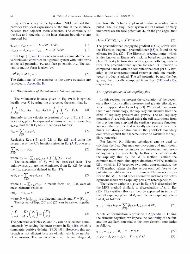
In Fig. 1a, the analytical solution and the FD and MFE-DG solutions at different times are plotted. In this simplecase of a 1D homogeneous medium, the MFE-DG method

Table 1Relevant data for Example 1

Domain dimensions 300 m · 1 m · 1 mRock properties / = 0.2, k = 1 md

Fluid properties lw (cP)/ln (cP) = 1/1, 2/1, 2/3qw = qn = 1000 kg/m3

Relative permeabilities Linear, quadratic (Eq. (35))Capillary pressure NeglectedResidual saturations Srw = 0, Srn = 0.2Injection rate 5 · 10�4 PV/dayMesh size 80 cells

shows less numerical dispersion than the FD solution asexpected; both solutions are obtained on a uniform meshof 80 cells. Very fine gridding is needed by the FD methodto match the MFE-DG solution [40]. The superiority in ourmethod comes from using higher-order (linear) approxima-tions with the DG method, while piecewise constantapproximations are used with the FD method.

There are some special conditions where the FDmethod results in low numerical dispersion. If the dis-placing fluid is more viscous than the fluid being dis-placed and linear relative permeabilities are used, theanalytical solution has one shock similar to the previouscase. The numerical dispersion is, however, low, asshown in Fig. 1b.

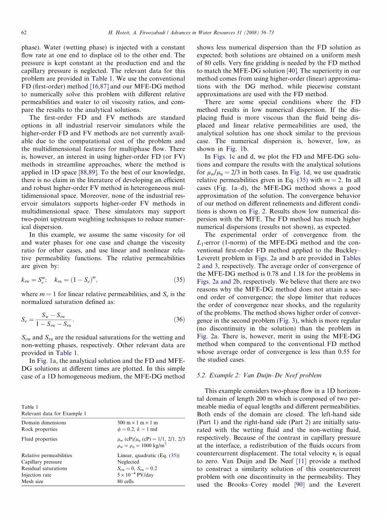
In Figs. 1c and d, we plot the FD and MFE-DG solu-tions and compare the results with the analytical solutionsfor lw/ln = 2/3 in both cases. In Fig. 1d, we use quadraticrelative permeabilities given in Eq. (35) with m = 2. In allcases (Fig. 1a–d), the MFE-DG method shows a goodapproximation of the solution. The convergence behaviorof our method on different refinements and different condi-tions is shown on Fig. 2. Results show low numerical dis-persion with the MFE. The FD method has much highernumerical dispersions (results not shown), as expected.

The experimental order of convergence from theL1-error (1-norm) of the MFE-DG method and the con-ventional first-order FD method applied to the Buckley–Leverett problem in Figs. 2a and b are provided in Tables2 and 3, respectively. The average order of convergence ofthe MFE-DG method is 0.78 and 1.18 for the problems inFigs. 2a and 2b, respectively. We believe that there are tworeasons why the MFE-DG method does not attain a sec-ond order of convergence; the slope limiter that reducesthe order of convergence near shocks, and the regularityof the problems. The method shows higher order of conver-gence in the second problem (Fig. 3), which is more regular(no discontinuity in the solution) than the problem inFig. 2a. There is, however, merit in using the MFE-DGmethod when compared to the conventional FD methodwhose average order of convergence is less than 0.55 forthe studied cases.

5.2. Example 2: Van Duijn–De Neef problem

This example considers two-phase flow in a 1D horizon-tal domain of length 200 m which is composed of two per-meable media of equal lengths and different permeabilities.Both ends of the domain are closed. The left-hand side(Part 1) and the right-hand side (Part 2) are initially satu-rated with the wetting fluid and the non-wetting fluid,respectively. Because of the contrast in capillary pressureat the interface, a redistribution of the fluids occurs fromcountercurrent displacement. The total velocity vt is equalto zero. Van Duijn and De Neef [11] provide a methodto construct a similarity solution of this countercurrentproblem with one discontinuity in the permeability. Theyused the Brooks–Corey model [90] and the Leverett

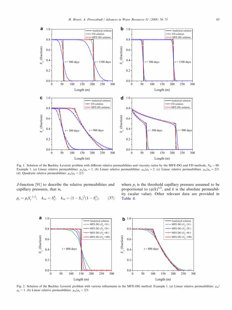
Fig. 1. Solution of the Buckley–Leverett problem with different relative permeabilities and viscosity ratios by the MFE-DG and FD methods, NK = 80:Example 1. (a) Linear relative permeabilities: lw/ln = 1. (b) Linear relative permeabilities: lw/ln = 2. (c) Linear relative permeabilities: lw/ln = 2/3.(d). Quadratic relative permeabilities: lw/ln = 2/3.


J-function [91] to describe the relative permeabilities andcapillary pressures, that is,

pc ¼ ptS�1=2e ; krw ¼ S4

e ; krn ¼ ð1� SeÞ2ð1� S2eÞ; ð37Þ

Fig. 2. Solution of the Buckley–Leverett problem with various refinements inln = 1. (b) Linear relative permeabilities: lw/ln = 2/3.

where pt is the threshold capillary pressure assumed to beproportional to (//k)1/2, and k is the absolute permeabil-ity (scalar value). Other relevant data are provided inTable 4.

the MFE-DG method: Example 1. (a) Linear relative permeabilities: lw/

Table 2Convergence order of the MFE-DG method and the conventional FDmethod applied to the Buckley–Leverett problem as given in Fig. 2a(Example 1)

MFE-DG method FD method

Gridblocks L1-error Order L1-error Order

20 0.016 0.04040 0.010 0.69 0.030 0.41

80 0.006 0.74 0.022 0.41

160 0.003 0.92 0.015 0.55

Table 3Convergence order of the MFE-DG method and the conventional FDmethod applied to the Buckley–Leverett problem as given in Fig. 2b(Example 1)

MFE-DG method FD method

Gridblocks L1-error Order L1-error Order

20 0.011 0.03540 0.005 1.18 0.025 0.48

80 0.002 1.27 0.017 0.55

160 0.001 1.10 0.011 0.62


The authors neglected the hysteresis in the capillarypressures and relative permeabilities. They used the samecapillary pressure functions for the imbibition and drain-age processes. However, the problem is of interest for thepurpose of verifying our numerical model. Let (kl,kr) and(pt,l,pt,r) be the relative permeabilities and the thresholdpressures in Part 1 (left) and Part 2 (right), respectively.In this example, we compare the MFE-DG solutions tosemi-analytical solution for different permeability distri-butions (Cases A–D), where we get a continuity in cap-illary pressure in Cases A–C and discontinuity in CaseD.

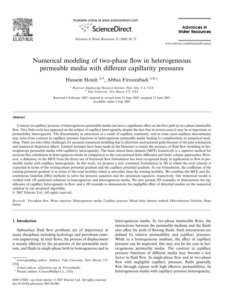
Case A: We consider the same properties for the twomedia, that is, kl/kr = 1 and pt,l/pt,r = 1. Theproblem becomes similar to the countercurrentdisplacement in a homogeneous medium byMcWhorter and Sunada [92], and Kashchievand Firoozabadi [93]. The boundary conditionsare, however, different. The MFE-DG solutionand the semi-analytical solutions at differenttimes are plotted in Fig. 3a. In this case, the cap-


Domain dimensions 200 m

Rock properties / = 0.42.9/85

Fluid properties lw = lRelative permeabilities BrookCapillary pressure LavereResidual saturations Srw =Injection rate 0Mesh size 100 ce

illary pressure and the saturation are both con-tinuous in the domain. The MFE-DG solutioncorrectly matches the semi-analytical solutionon a uniform mesh of 100 cells (gridding is sim-ilar for Case A and the other three cases). Thedomain is discretized in such a way that theinterface between the two media coincides withthe numerical cells.

Case B: We use the less permeable medium in Part 1. Thepermeability and threshold pressure ratios are kl/kr = 1/2 and pt;l=pt;r ¼

ffiffiffi2p

, respectively. Becauseof the difference in capillary pressure functions,there is a discontinuity in saturation at the inter-face between the two parts. Let I denote the inter-face between the two media located at the middleof the domain (x = 100 m), and Sw,l and Sw,r bethe left- and right-hand sides of the wetting phasesaturation at I. The capillary pressure is alwayscontinuous across the heterogeneity interfaceexcept when one phase is immobile [3,11,30].The continuity of capillary pressures at I isexpressed by:

pcIðSw;lÞ ¼ pcI

ðSw;rÞ: ð38Þ

A discontinuity in the capillary pressure occurswhen for a given Sw,l, there is no feasible valueof Sw,r that satisfies the continuity condition inEq. (38). The upper capillary pressure functionin Fig. 4a corresponds to the fine medium (Part1) and the lower function corresponds to thecoarse medium (Part 2). When flow occurs, thewetting phase saturation Sw,l decreases and Sw,r

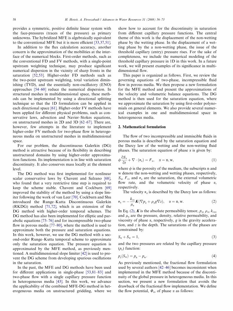
increases. Following the upper capillary pressurecurve, pc,l, in Fig. 4a in the decreasing direction ofSw,l, there always exists a right-hand side satura-tion, Sw,r, that satisfies Eq. (38). The capillarypressure is, therefore, continuous. Fig. 3b showsgood agreement between the MFE-DG solutionand the semi-analytical solution of the wetting-phase saturation at different times.

Case C: In this case, unlike the previous one, we use amore permeable medium in Part 1. The perme-ability and threshold capillary pressure ratiosare kl/kr = 2 and pt;l=pt;r ¼ 1=

ffiffiffi2p

, respectively.Van Duijn et al. [3,11] showed that there is a

· 1 m · 1 m

25, kl (d)/kr (d) = 85.8/85.8,.8, 85.8/42.9, 85.8/21.45

n = 1 cP, qw = qn = 1000 kg/m3

s–Corey model Eq. (37))tt model (Eq. (37)), pt,l (bar)/pt,r (d)=0.1/0.1, 0.141/0.1, 0.1/0.141, 0.1/0.20, Srn = 0

lls

Fig. 3. Solution of the Van Duijn–De Neef problem at different times with different permeabilities and capillary pressures by the MFE-DG method,NK = 100: Example 2. (a) kl/kr = 1; pt,l/pt,r = 1. (b) kl=kr ¼ 1=2; pt;l=pt;r ¼

ffiffiffi2p

. (c) kl=kr ¼ 2; pt;l=pt;r ¼ 1=ffiffiffi2p

. (d) kl/kr = 4; pt,l/pt,r = 1/2.


critical saturation S�w, with pc;lðS�wÞ ¼ pc;rð1Þ, suchthat Eq. (38) is satisfied if Sw,l (t > 0) is less thanS�w (see Fig. 4b). The authors provided a methodto calculate Sw,l(t > 0), which depends on thethreshold capillary pressure ratios and the typeof the capillary pressure functions. In this case,Sw;l < S�w; as a result there is continuity in capil-lary pressure. Fig. 3c shows the saturation profilesat different times versus the domain length. The

Fig. 4. Capillary-pressure functions in the left- (Part 1) and right-hand (Part 2)Example 2. (a) pt;l=pt;r ¼

ffiffiffi2p

. (b) pt;l=pt;r ¼ 1=ffiffiffi2p

. (c) pt,l/pt,r = 2.

MFE-DG solution is in agreement with thesemi-analytical solutions without imposing anyadditional conditions other than the continuityof the flux and capillarity pressure given in Eqs.(29) and (30).

Case D: We increase the permeability and capillary pres-sure contrast between the two media (kl/kr = 4and pt,l/pt,r = 1/2). The left-hand saturation isgreater than S�w ¼ 1=4 (see Fig. 4c); therefore,

of the media vs. the wetting-phase saturation for different rock properties:


continuity in the capillary pressure cannot beestablished. At time t > 0, we get a jump in theright-hand saturation to one, that is Sw,r = 1[3,11]. In this case, the continuity condition ofthe capillary pressure in our numerical methodgiven in Eq. (30) is not valid. We relaxed the con-tinuity constraint by allowing two different valuesof the capillary pressure at I. The system can beclosed from the knowledge of the right-hand sat-uration, that is, pc,r = pc,r(1) = pt,r. The jumps inthe saturations at different times appear inFig. 3d. The MFE-DG solution can describe cor-rectly the left-hand jump in saturation; our calcu-lated results are in agreement with the semi-analytical solutions.

Fig. 5. Two-dimensional domains with heterogeneous permeabilities: E

Table 5Relevant data for Examples 3a and 3b

Example 3a

Domain dimensions 500 m · 270 m · 1 mRock properties / = 0.2, k = 1, 100

Fluid properties lw = 1 cP, ln = 0.4qw = 1000 kg/m3, q

Relative permeabilities Quadratic (Eq. (35)Capillary pressure Bc = 5, 50 bar (Eq.Residual saturations Srw = 0, Srn = 0Injection rate 0.11 PV/yearMesh size 4500 rectangles

Wid

th (

m)

0

30

60

90

120

150

180

210

240

270

0.900.800.700.600.500.400.300.200.10

Sw(fraction)

Length (m)0 100 200 300 400 500

Fig. 6. Wetting-phase saturation profiles at 0.5 PVI with zero and nonzerocapillary pressure.

5.3. Example 3: effect of capillarity on flow in heterogeneous

media

In this example, we show the significance of capillarypressure contrast in heterogeneous media. We consider a2D horizontal domain with two different configurationsfor the permeability distribution. In the first configuration(Example 3a), the domain is composed of layers of alter-nate permeabilities (1 md and 100 md), as shown inFig. 5a. Water (wetting phase) is uniformly injected acrossthe left-hand side of the layered domain, which is initiallysaturated with oil (non-wetting phase). The production isacross the opposite right-hand side. The injection rate inpore volume (PV) is 0.11 PV/year. The capillary pressure-saturation function is given by:

xample 3. (a) Layered heterogeneities. (b) Random heterogeneities.

Example 3b

500 m · 270 m · 1 mmd / = 0.2, k = 0.1–100 md

5 cP, As in Example 3a

n = 660kg/m3

) As in Example 3a(39)) Bc = 1–33 bar (Eq. (39))

As in Example 3a0.06 PV/year3158 triangles

Wid

th (

m)

0

30

60

90

120

150

180

210

240

270Sw(fraction)

0.900.850.800.700.600.500.400.300.200.10

Length (m)0 100 200 300 400 500

capillary pressure: Example 3a. (a) Zero capillary pressure. (b) Nonzero

0.900.850.800.700.600.500.400.300.200.10

Sw(fraction)

0.900.850.800.700.600.500.400.300.200.10

Sw (fraction)W

idth

(m

)

0

30

60

90

120

150

180

210

240

270

Length (m)0 100 200 300 400 500

Wid

th (

m)

0

30

60

90

120

150

180

210

240

270

Length (m)0 100 200 300 400 500

Fig. 7. Wetting-phase saturation profiles at 0.5 PVI with homogeneous and heterogeneous capillary pressure functions: Example 3b. (a) Homogeneouscapillary pressure. (b) Heterogenous capillary pressure.

Table 6Computational CPU time for the problem in Example 3 that correspondto Figs. 5a and b and 6a and b

Fig. 5a Fig. 5b Fig. 6a Fig. 6b

Time(s) 105 152 141 169


Domain dimensions 200 m · 400 m · 200 mRock properties / = 0.2, k=1 mdFluid properties As in Example 3aRelative permeabilities Cubic (Eq. (35))Capillary pressure NeglectedResidual saturations Srw = 0.1, Srn = 0.1Injection rate 0.0625 PV/dayMesh size 4500 hexahedrons, 4760 prisms


pcðSeÞ ¼ �Bc log Se; ð39Þwhere the capillary pressure parameter Bc is inversely pro-portional to

ffiffiffikp

.The relative permeabilities are quadratic function of

water saturation. Other relevant parameters are providedin Table 5. In Fig. 6, we compare the calculated wetting-phase saturation with and without capillary pressure at0.5 pore volume injection (PVI). In Fig. 6a, with zero cap-illary pressure, the injected water flows faster in the morepermeable layers, as expected. In Fig. 6b, where we takethe capillary pressure into account, the flow in the morepermeable layers slows down because of the cross-flowbetween the layers owing to the contrast in capillary pres-sure. A two-phase flow occurs in the transverse directionsof the adjacent layers in a very narrow region similar tothe one observed in fractured media [94]. In this example,the capillary pressure is continuous because the thresholdcapillary pressure is zero, as described in Eq. (39).

In the second configuration, we use a random distribu-tion of permeabilities in the domain, as shown in Fig. 5b.Water is injected at one corner to displace oil to the oppo-site corner with a constant injection rate of 0.06 PV/year.The capillary pressure and the relative permeability modelsare the same as in Example 3a (Table 5). In Fig. 7a, weshow the water saturation profile at PV = 0.5 by consider-ing a single capillary pressure function for the wholedomain. The capillary pressure parameter Bc is computedusing an arithmetic average permeability equal to 0.5 md.The water saturation profile presented in Fig. 7b is calcu-lated at PV = 0.5 by considering different capillary pressurefunctions corresponding to different permeabilities. Thereis a significant effect of the capillary pressure contrast thatleads to a less diffusive solution and, therefore, a more effi-cient recovery. Note that unlike in homogeneous media,where capillary pressure results in a diffusive front, in het-erogeneous media with capillary pressure contrast the frontmay become less diffusive. We like to emphasize that whena single capillary pressure function is assigned to a hetero-geneous media, there is very little effect on flow on the typeof problems discussed in this work.

The computational time for all cases in this example aregiven in Table 6. The increase in CPU time when the cap-illary pressure is taken into account is due to the increase innonlinearity of the problem that affects the size of timestep.

5.4. Example 4: effect of mesh on the MFE method

The purpose of this last example is to show the robust-ness of the MFE method on unstructured meshes with lowquality. We consider a 3D tilted domain with dimension(200 m · 400 m · 200 m). The injection and productionwells are located at the coordinates (0, 0,0), and (200 m,400 m,200 m), respectively. The injection rate is 0.0625PV/day. The rock and fluid properties are provided inTable 7. We consider different mesh types made of hexahe-drons and prisms and examine the effect of mesh quality onthe recovery and the saturation distribution. In Figs. 8aand 8c, we discretize the 3D domain into meshes made of

X(m)

0

100

200

Y(m

)

0

100

200

300

400

Z(m

)

0

100

200

300

X

YZ

X(m)

0

100

200

Y(m

)

0

100

200

300

400

Z(m

)

0

100

200

300

X

YZ

X(m)

0

100

200

Y(m

)

0

100

200

300

400

Z(m

)

0

100

200

300

X

YZ

X(m)

0

100

200

Y(m

)

0

100

200

300

400

Z(m

)

0

100

200

300

X

YZ

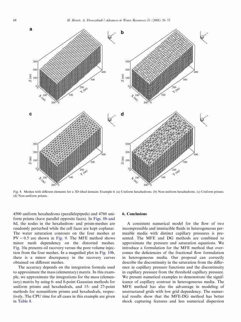
Fig. 8. Meshes with different elements for a 3D tilted domain: Example 4. (a) Uniform hexahedrons. (b) Non-uniform hexahedrons. (c) Uniform prisms.(d) Non-uniform prisms.


4500 uniform hexahedrons (parallelepipeds) and 4760 uni-form prisms (have parallel opposite faces). In Figs. 8b and8d, the nodes in the hexahedron- and prism-meshes arerandomly perturbed while the cell faces are kept coplanar.The water saturation contours on the four meshes atPV = 0.5 are shown in Fig. 9. The MFE method showsminor mesh dependency on the distorted meshes.Fig. 10a presents oil recovery versus the pore volume injec-tion from the four meshes. In a magnified plot in Fig. 10b,there is a minor discrepancy in the recovery curvesobtained on different meshes.

The accuracy depends on the integration formula usedto approximate the mass (elementary) matrix. In this exam-ple, we approximate the integrations for the mass (elemen-tary) matrix by using 6- and 8-point Gaussian methods foruniform prisms and hexahedrals, and 15- and 27-pointmethods for nonuniform prisms and hexahedrals, respec-tively. The CPU time for all cases in this example are givenin Table 8.

6. Conclusions

A consistent numerical model for the flow of twoincompressible and immiscible fluids in heterogeneous per-meable media with distinct capillary pressures is pre-sented. The MFE and DG methods are combined toapproximate the pressure and saturation equations. Weintroduce a formulation for the MFE method that over-comes the deficiencies of the fractional flow formulationin heterogeneous media. Our proposal can correctlydescribe the discontinuity in the saturation from the differ-ence in capillary pressure functions and the discontinuityin capillary pressure from the threshold capillary pressure.We present numerical examples to demonstrate the signif-icance of capillary contrast in heterogeneous media. TheMFE method has also the advantage in modeling ofunstructured grids with low grid dependency. The numer-ical results show that the MFE-DG method has bettershock capturing features and less numerical dispersion

Fig. 10. Recovery of the non-wetting phase vs. PV injection with different gridings in the MFE-DG method: Example 4.

X(m)

0

100

200

Y(m

)

0

100

200

300

400

Z(m

)

0

100

200

300

X

YZ

0.85

0.80

0.72

0.70

0.50

0.40

0.20

Sw

(fraction)

X(m)

0

100

200

Y(m

)

0

100

200

300

400

Z(m

)

0

100

200

300

X

YZ

0.85

0.80

0.72

0.70

0.50

0.40

0.20

Sw(fraction)

X(m)

0

100

200

Y(m

)

0

100

200

300

400

Z(m

)

0

100

200

300

X

YZ

0.85

0.80

0.72

0.70

0.50

0.40

0.20

Sw

(fraction)

X(m)

0

100

200

Y(m

)

0

100

200

300

400

Z(m

)

0

100

200

300

X

YZ

0.85

0.80

0.72

0.70

0.50

0.40

0.20

Sw

(fraction)

Fig. 9. Wetting-phase saturation profiles at 0.5 PVI with different meshes: Example 4. (a) Uniform hexahedrons. (b) Non-uniform hexahedrons. (c)Uniform prisms. (d) Non-uniform prisms.

Table 8Computational CPU time for the problem in Example 4 that correspondto Figs. 9a–d

Fig. 9a 9b Fig. 9c Fig. 9d

Time (s) 523 575 757 797


than the first-order FD method. In a forthcoming work,we will demonstrate major advantages of the combinedMFE-DG method in fractured media for immiscibletwo-phase flow.


Appendix A. The Raviart–Thomas basis functions

The Raviart–Thomas (RT0) space defines the velocityvector over each cell K in terms of the fluxes across the cellfaces E. The RT0 basis functions are available for all stan-dard geometrical elements (see Fig. A.1). The basis func-tions for the hexahedral, prismatic, and tetrahedralreference elements are given below in following equations,respectively.

wEi ;i¼1;...;6 :

u

0

0

0B@1CA; u� 1

0

0

0B@1CA; 0

v

0

0B@1CA; 0

v� 1

0

0B@1CA;

0

0

f

0B@1CA; 0

0

f� 1

0B@1CA:

ðA:1Þ

wEi ;i¼1;...;5 :

u

v� 1

0

0B@1CA; u� 1

v

0

0B@1CA; u

v

0

0B@1CA; 2

0

0

f

0B@1CA;

2

0

0

f� 1

0B@1CA:

ðA:2Þ

wEi ;i¼1;...;4 : 2

u

v� 1

f

0B@1CA; 2

u� 1

v

f

0B@1CA; 2

u

v

f

0B@1CA;

2

u

v

f� 1

0B@1CA:

ðA:3Þ

The basis functions are linearly independent and satisfy thefollowing properties:

r � wE ¼1

jKj ; wE:nE0 ¼1=jEj if E ¼ E0;

0 if E 6¼ E0;

�ðA:4Þ

where |K| and |E| are the volume and the area of the cell Kand face E, respectively. In 2D, similar relations apply.

6

v

ζ

1

E

E

w

w33

44 1

u10

E2 w2 1E1w

E5w5

E6

w

4

ζE

E

E

w

ww

1

1

0

11

E

w2

4

5

5

2

Fig. A.1. Raviart–Thomas basis functions on hexahed

A velocity vector vK over K can be uniquely written interms of the fluxes qK,E across edge(face) E and the basisfunctions given in Eqs. (A.1)–(A.3):

vK ¼XE2oK

qK;EwE; ðA:5Þ

where oK = {Ei; i = 1,. . .,Ne}.

Appendix B. Discretization of the velocity va

Eq. (15) can be written for all faces E in K in the matrixform:

AKQa;K ¼ Uw;Ke� Kw;K ; ðB:1Þ

whereAK = [AK,E,E 0]E,E 02oK; Qa,K = [qa,K,E]E2oK; Kw,K =[Kw,K,E]E2oK; e = [1]E2oK.

The matrix AK is symmetric and positive definite. Byinverting AK, Eq. (B.1) becomes:

Qa;K ¼ Uw;KA�1K e� A�1

K KK : ðB:2Þ

Eq. (17) can be obtained by expanding Eq. (B.1). The coef-ficients bK,E and aK,E in Eq. (17) and aK in Eq. (24) are de-fined by:

bK;E;E0 ¼ A�1K;E;E0 ; aK;E ¼

XE02oK

bK;E;E0 ; aK ¼XE2oK

aK;E

In Eq. (20), R is an NK · NE rectangular matrix, M is anNE · NE square matrix, and V is a vector of size NE thatdescribes the boundary conditions. The entities of R andM are:

R ¼ ½RK;E�NK ;NE; RK;E ¼ aK;E E 2 oK;

M ¼ ½ME;E0 �NE ;NE; ME;E0 ¼

XE;E03oK

bK;E;E0 E 62 CD;

V ¼ ½V E�NE; V E ¼

XE02oK\CD

bK;E;E0Kw;E0 :

ðB:3Þ

Appendix C. Discretization of the velocity vc

The velocity variables va and vc have similar forms (seeEq. (7)). However, unlike the coefficient kt in va, the mobil-ity coefficient kn in vc can be zero and so it cannot beinverted as in Eq. (14). We multiply vc by the inverse matrixof KK to obtain:

K�1K vc;K ¼ �knrUc: ðC:1Þ

v

u

Ew

1

33

2

ζ

1

u10

vwE

wE

w E

wE

1 1

2

33

44

1

ral, prismatic, and tetrahedral reference elements.


Following a similar procedure used for Eqs. (15) and (16)(see Appendix B), one gets:

qc;K;E ¼ kn;E

XE02oK

bA�1K;E;E0Uc;K �

XE02oK

bA�1K;E;E0Kc;K;E0

!; E 2 oK;

ðC:2Þwhere bAK;E;E0 ¼

R R RK wK;EK�1

K wK;E0 .In the above equation, kn;E is the non-wetting phase

mobility at the interface E of a cell K and the neighboringcell K 0 (E = K \ K 0). The interface mobility is calculatedfrom data in the upstream cell, that is:

kn;E ¼kn;K;E if qc;E P 0 ði:e:; effluxÞ;kn;K 0 ;E if qc;E < 0 ði:e:; influxÞ:

(ðC:3Þ

The flux qc,E in Eq. (C.3) is known from the previous timestep. Between homogeneous cells, the mean value weight-ing technique can also be used instead of the fully upstreamtechnique in Eq. (C.3). The coefficients bK;E;E0 and aK;E inEq. (28) are defined by:

bK;E;E0 ¼ kn;K;EbA�1

K;E;E0 ; aK;E ¼ kn;K;E

XE02oK

bA�1K;E;E0 :

Appendix D. Slope limiter

We use the multidimensional slope limiter introduced byChavent and Jaffre [42]. It is formulated in such a way toavoid local minima or maxima at the grid nodes. In eachcell K, the saturation variable at a vertex i should be withinthe minimum and the maximum of the cell-average satura-tions of all neighboring elements. Let Ti be the set of allcells having i as a vertex. We define the notation:

Sw;K ¼1

jKj

Z Z ZK

Sw;K ; fSw;Kg; Sw;mini¼ min

K2T iSw;max

i

¼ maxK2T i

fSw;Kg:

Then, Sw;K ¼ LðeSw;KÞ is the solution of the following least-squares problem:

minW2Rnv

kW � eSw;Kk;

with the linear constraints :

W ¼ 1nv

Pnv

i¼1

W i ¼ Sw;K ;

Sw;mini6 W i 6 Sw;max;i; i ¼ 1; . . . ; nv:

8>>>>>>><>>>>>>>:ðD:1Þ

In the minimization problem in Eq. (D.1), we seek the clos-est solution, Sw,K = W, to the initial distribution of satura-tion, eSw;K , in K that keeps the same total material and is freefrom local minima and maxima at the nodes. The problemcan be solved efficiently by using an iterative procedure[42,95] that requires at most 2nv iterations to converge.

We note that the Chavent-Jaffre slope limiter in [42] hasa tuning parameter a 2 [0,1] that controls the degree ofrestriction of the slopes. The parameter a does not appearin our definition in Eq. (D.1) as it is set to one.

References

[1] Yoshio Y, Lake L. The effects of capillary pressure on immiscibledisplacements in stratified porous media. In: Annual technicalconference and exhibition, No. SPE10109; 1981.

[2] Chaouche M, Rakotomalala N, Salin D, Xu B, Yortsos Y. Capillaryeffects in drainage in heterogeneous porous media: continuummodelling, experiments and pore network simulations. Chem EngSci 1994;49(15):2447–66.

[3] Van Duijn C, Molenaar J, De Neef M. The effect of capillary forceson immiscible two-phase flow in heterogeneous porous media.Transport Porous Media 1995;21(1):71–93.

[4] Parsons I, Coutinho A. Finite element multigrid methods for two-phase immiscible flow in heterogeneous media. Commun NumerMethods Eng 1999;15(1):1–7.

[5] Christie M, Blunt M. Tenth SPE comparative solution project: acomparison of upscaling techniques. SPE J 2001;4(2):308–17.

[6] Jenny P, Wolfsteiner C, Lee S, Durlofsky L. Modeling flow ingeometrically complex reservoirs using hexahedral multiblock grids.SPE J 2002;7(2):149–57.

[7] Tchelepi H, Jenny P, Zurich E, Lee S, Wolfsteiner C. An adaptivemultiphase multiscale finite volume simulator for heterogeneousreservoirs. In: Reservoir simulation symposium, No. SPE93395; 2005.

[8] Zhang P, Pickup G, Christie M. A new upscaling approach for highlyheterogeneous reservoirs. In: Reservoir simulation symposium, No.SPE93395; 2005.

[9] Lunati I, Jenny P. Multiscale finite-volume method for compress-ible multiphase flow in porous media. J Comput Phys 2006;216(2):616–36.

[10] Yortsos Y, Chang J. Capillary effects in steady-state flow inheterogeneous cores. Transport Porous Media 1990;5(4):399–420.

[11] Van Duijn C, De Neef M. Similarity solution for capillary redistri-bution of two phases in a porous medium with a single discontinuity.Adv Water Res 1998;21(6):451–61.

[12] Niessner J, Helmig R, Jakobs H, Roberts J. Interface condition andlinearization schemes in the newton iterations for two-phase flow inheterogeneous porous media. Adv Water Res 2005:671–87.

[13] Reichenberger V, Jakobs H, Bastian P, Helmig R. A mixed-dimensional finite volume method for multiphase flow in fracturedporous media. Adv Water Res 2006:1020–36.

[14] Beveridge S, Coats K, Agarwal R, Modine A. A study of thesensitivity of oil recovery to production rate. In: Annual technicalconference and exhibition, No. SPE5129; 1974.

[15] Correa A, Firoozabadi A. Concept of gravity drainage in layeredporous media. SPE J 1990(March):101–11.

[16] Aziz K, Settari A. Petroleum reservoir simulation, environmentalengineering. London: Elsevier Applied Science Publishers; 1979.

[17] Helmig R. Multiphase flow and transport processes in the subsurface.A contribution to the modeling of hydrosystems, environmentalengineering. Berlin: Springer Verlag; 1997.

[18] Coats K, Thomas K, Pierson R. Compositional and black oilreservoir simulation. SPE Reservoir Evaluat Eng 1998;1(4):372–9.

[19] Brand W, Heinemann J, Aziz K. The grid orientation effect inreservoir simulation. In: Symposium on reservoir simulation, No.SPE21228; 1991.

[20] Nacul E, Aziz K. Use of irregular grid in reservoir simulation. In:Annual technical conference and exhibition, No. SPE22886; 1991.

[21] Aavatsmark I, Barkve T, Bœ O, Mannseth T. Discretization on non-orthogonal, quadrilateral grids for inhomogeneous, anisotropicmedia. J Comput Phys 1996;127(1):2–14.

[22] Gunasekera D, Childs P, Herring J, Cox J. A multi-point fluxdiscretization scheme for general polyhedral grids. In: Internationaloil and gas conference and exhibition, No. SPE48855; 1998.

[23] Aavatsmark I. An introduction to multipoint flux approximations forquadrilateral grids. Comput Geosci 2002;6(3):405–32.

[24] Juanes R, Kim J, Matringe S, Thomas K. Implementation andapplication of a hybrid multipoint flux approximation for reservoir


simulation on corner-point grids. In: Annual Technical Conferenceand Exhibition, No. SPE95928; 2005.

[25] Nordbotten J, Brunsgt J. Discretization on quadrilateral grids withimproved monotonicity properties. J Comput Phys2002;203(2):744–60.

[26] Heinemann Z, Brand C, Munka M, Chen Y. Modeling reservoirgeometry with irregular grids. SPE J 1991(May):225–32.

[27] Eymard R, Sonier F. Mathematical and numerical properties ofcontrol-volume finite-element scheme for reservoir simulation. SPE J1994;9(4):283–9.

[28] Geiger S, Roberts S, Matth S, Zoppou C, Burri A. Combining finiteelement and finite volume methods for efficient multiphase flowsimulations in highly heterogeneous and structurally complex geo-logic media. Geofluids 2004;4(4):284–99.

[29] Monteagudo J, Firoozabadi A. Control-volume model for simulationof water injection in fractured media: incorporating matrix hetero-geneity and reservoir wettability effects. SPE J; in press.

[30] Helmig R, Huber R. Comparison of Galerkin-type discretizationtechniques for two-phase flow in heterogeneous porous media. AdvWater Res 1998;21(8):697–711.

[31] Thomas J. Sur l’analyse numerique des methodes d’element finishybrides et mixtes. Ph.D. thesis, Univ. de Pierre et Marie Curie,France; 1977.

[32] Raviart P, Thomas J. A mixed hybrid finite element method for thesecond order elliptic problem. Lectures notes in mathematics606. New York: Springer-Verlag; 1977.

[33] Brezzi F, Fortin M. Mixed and hybrid finite element methods,environmental engineering. New York: Springer-Verlag; 1991.

[34] Durlofsky L. Accuracy of mixed and control volume finite elementapproximations to darcy velocity and related quantities. WaterResour Res 1994;30(4):965–73.

[35] Mose R, Siegel P, Ackerer P, Chavent G. Application of the mixed-hybrid finite element approximation in a ground water flow model:luxury or necessity? Water Resour Res 1994;30(11):3001–12.

[36] Darlow B, Ewing R, Wheeler M. Mixed finite element method formiscible displacement problems in porous media. SPE J1984;24:391–8.

[37] Chavent G, Roberts J. A unified physical presentation of mixed,mixed-hybrid finite element method and standard finite differenceapproximations for the determination of velocities in water flowproblems. Adv Water Res 1991;14(6):329–33.

[38] Yotov I. Mixed finite element methods for flow in porous media,Ph.D. thesis, Rice University, Houston, TX; 1996.

[39] Arbogast T, Wheeler M, Yotov I. Mixed finite elements for ellipticproblems with tensor coefficients as cell-centered finite differences.SIAM J Numer Anal 1997;34(2):828–85.

[40] Hoteit H, Firoozabadi A. Multicomponent fluid flow by discontin-uous Galerkin and mixed methods in unfractured and fracturedmedia. Water Resour Res 2005;41(11):W11412.

[41] Chavent G, Cohen G, Jaffre J, Dupuy M, Ribera I. Simulation oftwo-dimensional waterflooding by using mixed finite elements. SPE J1984:382–90.

[42] Chavent G, Jaffre J. Mathematical models and finite elements forreservoir simulation. Studies in mathematics and its applica-tions. North-Holland: Elsevier; 1986.

[43] Chavent G, Cohen G, Jaffre J, Eyard R, Dominique R, Weill L.Discontinuous and mixed finite elements for two-phase incompress-ible flow. SPE J 1990(November):567–75.

[44] Ewing R, Heinemann R. Incorporation of mixed finite elementmethods in compositional simulation for reduction of numericaldispersion. In: Reservoir simulation symposium, No. SPE12267;1983.

[45] Chen Z, Ewing R. From single-phase to compositional flow:applicability of mixed finite elements. Transport Porous Media1997;57:225–42.

[46] Chen Z, Ewing R, Jiang Q, Spagnuolo A. Degenerate two-phaseincompressible flow V: characteristic finite element methods. J NumerMath 2002;10(2):87–107.

[47] Chavent G, Jaffre J, Roberts J. Generalized cell-centered finitevolume methods: application to two-phase flow in porous media. In:Computational science for the 21st Century, Chichester, England;1997. p. 231–41.

[48] Nayagum D, Schafer G, Mose R. Modelling two-phase incompress-ible flow in porous media using mixed hybrid and discontinuous finiteelements. Comput Geosci 2004;8(1):49–73.

[49] Chen H, Chen Z, Huan G. Mixed discontinuos finite elementmethods for multiphase flow in porous media. J Comput Methods SciEng 2001;2(3):1–13.

[50] Durlofsky L. A triangle based mixed finite element-finite volumetechnique for modeling two phase flow through porous media. JComput Phys 1993;105(2):252–66.

[51] Hoteit H, Erhel J, Mose R, Bernard P, Ackerer P. Numericalreliability for mixed methods applied to flow problems in porousmedia. Comput Geosci 2002;6(2):161–94.

[52] Coats K. An equation of state compositional model. SPE J1980:363–76.

[53] Hoteit H, Firoozabadi A. Compositional modeling by the com-bined discontinuous Galerkin and mixed methods. SPE J2006;11(1):19–34.

[54] Todd M, O’Dell P, Hirasaki G. Methods for increased accuracy innumerical reservoir simulators. SPE J 1972(December):515–30.

[55] Holloway C, Thomas K, Pierson R. Reduction of grid orientationeffects in reservoir simulation. In: Annual technical conference andexhibition, No. SPE5522; 1975.

[56] Harten A. High resolution schemes for hyperbolic conservation laws.J Comput Phys 1983;49(2):357–93.

[57] Sweby P. High resolution schemes using flux limiters for hyperbolicconservation laws. SIAM J Numer Anal 1984;21:995–1011.

[58] Osher S, Chakravarthy S. High resolution schemes and the entropycondition. SIAM J Numer Anal 1984;21(12):955–84.

[59] Harten A, Engquist B, Osher S, Chakravarthy S. Uniformly highorder accurate essentially non-oscillatory schemes. J Comput Phys1987;71(2):231–303.

[60] Shu C, Osher S. Efficient implementation of essentially non-oscilla-tory shock-capturing schemes. J Comput Phys 1987;77(2):439–71.

[61] Toro E. Riemann solver and numerical methods for fluids dynam-ics. Manchester: Springer; 1997.

[62] Kaser M, Iske A. ADER schemes on adaptive triangular meshes forscalar conservation laws. J Comput Phys 2004;205:486–508.

[63] Dumbser M, Kaser M. Arbitrary high order non-oscillatory finitevolume schemes on unstructured meshes for linear hyperbolicsystems. J Comput Phys 2006. doi:10.1016/j.jcp.2006.06.043.

[64] Ollivier-Gooch C, Van Altena M. A high-order-accurate unstructuredmesh finite-volume scheme for the advection diffusion equation. JComput Phys 2002;181:729–52.

[65] Hu C, Shu C. Weighted essentially non-oscillatory schemes ontriangular meshes. J Comput Phys 1999;150:97–127.

[66] Sonar T. On the construction of essentially non-oscillatory finitevolume approximations to hyperbolic conservation laws on generaltriangulations: polynomial recovery, accuracy and stencil selection.Comput Methods Appl Mech Engrg 1997;140:157–81.

[67] Kim D, Choi H. A second-order time-accurate finite volume methodfor unsteady incompressible flow on hybrid unstructured grids. JComput Phys 2000;162:411–28.

[68] Chavent G, Salzano A. A finite-element method for the 1-Dwater flooding problem with gravity. J Comput Phys 1982;45:307–44.

[69] Chavent G, Cockburn B. The local projection p0p1-discontinuousGalerkin finite element method for scalar conservation laws. M2AN1989;23:565–92.

[70] van Leer B. Towards the ultimate conservative scheme: II. J ComputPhys 1974;14:361–76.

[71] Cockburn B, Shu C. TVB Runge-Kutta local projection discontin-uous Galerkin finite element method for conservative laws II: generalframe-work. Math Comp 1989;52:411–35.

http://dx.doi.org/10.1016/j.jcp.2006.06.043


[72] Cockburn B, Shu C. The Runge-Kutta discontinuous Galerkinmethod for conservative laws V: Multidimensional systems. J ComputPhys 1998;141:199–224.

[73] Cockburn B, Shu C. The local discontinuous Galerkin finite elementmethod for convection–diffusion systems. SIAM J Numer Anal1998;35(6):2440–63.

[74] Oden J, Babuska I, Baumann C. A discontinuous hp finite elementmethod for diffusion problems. J Comput Phys 1998;146:491–519.

[75] Riviere B, Wheeler M, Girault V. Improved energy estimates forinterior penalty, constrained and discontinuous Galerkin methods forelliptic problems. Part I. Comput Geosci 1999;8:337–60.

[76] Arnold D, Brezzi F, Cockburn B, Marini L. Unified analysis ofdiscontinuous Galerkin methods for elliptic problems. SIAM JNumer Anal 2002;39(5):1749–79.

[77] Bastian P. Higher order discontinuous Galerkin methods for flow andtransport in porous media. In: Bansch E, editors. Challenges inscientific computing – CISC 2002, No. 35 in LNCSE; 2003. p. 1–22.

[78] Bastian P, Riviere B. Discontinuous Galerkin methods for two-phaseflow in porous media, Technical Report 28, IWR (SFB 359),Universitat Heidelberg; 2004.

[79] Riviere B. Numerical study of a discontinuous Galerkin method forincompressible two-phase flow. In: ECCOMAS Proceedings; 2004.

[80] Epshteyn Y, Riviere B. Fully implicit discontinuous finite elementmethods for two-phase flow. Appl Numer Math 2007(57):383–401.

[81] Siegel P, Mose R, Ackerer P, Jaffre J. Solution of the advection–dispersion equation using a combination of discontinuous and mixedfinite elements. Int J Numer Methods Fluids 2001;24:595–613.

[82] Bues M, Oltean C. Numerical simulations for saltwater intrusion bythe mixed hybrid finite element method and discontinuous finiteelement method. Transport Porous Media 2000;40(2):171–200.

[83] Hoteit H, Ackerer P, Mose R. Nuclear waste disposal simulations:couplex test cases. Comput Geosci 2004;8(2):99–124.

[84] Monteagudo J, Firoozabadi A. Control-volume method for numer-ical simulation of two-phase immiscible flow in two- and three-dimensional discrete-fractured media. Water Resour Res 2004;40(7):W07405.

[85] Eisenstat S. Efficient implementation of a class of preconditionedconjugate gradient methods. SIAM J Sci Stat Comput 1981;2:1–4.

[86] Buckley S, Leverett M. Mechanism of fluid displacement in sands.Trans AIME 1942;146:187–96.

[87] Peaceman D. Fundamentals of numerical reservoir simulation. NewYork: Elsevier Applied Science Publishers; 1977.

[88] Thiele M, Edwards M. Physically based higher order godunovschemes for compositional simulation. in: Reservoir simulationsymposiumm, No. SPE66403; 2001.

[89] Mallison B, Gerritsen M, Jessen K, Orr F. High order upwindschemes for two-phase, multicomponent flow. SPE J 2006(Septem-ber): 297–311.

[90] Brooks R, Corey A. Hydraulic properties of porous media. HydrolPap, vol.3. Fort Collins: Colorado State Univ.; 1964.

[91] Leverett M. Capillary behavior in porous solids. Trans AIME PetrEng Div 1941;142:152–69.

[92] McWhorter D, Sunada D. Exact integral solutions for two-phaseflow. Water Resour Res 1990;26(2):399–413.

[93] Kashchiev D, Firoozabadi A. Analytical solutions for 1dcountercurrent imbibition in water-wet media. SPE J 2003;8(4):401–8.

[94] Terez I, Firoozabadi A. Water injection in water-wet fracturedporous media: Experiments and a new model with modified Buckley–Leverett theory. SPE J 1999(June):134–41.

[95] Gowda V, Jaffre J. A discontinuous finite element method for scalarnonlinear conservation laws. Technical Report 1848, INRIA, France;1993.

Numerical modeling of two-phase ﬂow in heterogeneous ... · PDF filepermeable media with...

Documents

Transcript of Numerical modeling of two-phase ﬂow in heterogeneous ... · PDF filepermeable media with...