Numerical modeling of the geodynamo: Mechanisms of field

JOURNAL OF GEOPHYSICAL RESEARCH, VOL. 104, NO. B5, PAGES 10,383-10,404, MAY 10, 1999

Numerical modeling of the geodynamo' of field generation and equilibration

Mechanisms

Peter Olson

Department of Earth and Planetary Sciences, Johns Hopkins University, Baltimore, Maryland

Ulrich Christensen

Institut ffir Geophysik, Universitiit GSttingen, GSttingen, Germany

Gary A. Glatzmaier Earth Sciences Department, University of California, Santa Cruz

Abstract. Numerical calculations of fluid dynamos powered by thermal convection in a rotating, electrically conducting spherical shell are analyzed. We find two regimes of nonreversing, strong field dynamos at Ekman number 10 -4 and Rayleigh numbers up to 11 times critical. In the strongly columnar regime, convection occurs only in the fluid exterior to the inner core tangent cylinder, in the form of narrow columnar vortices elongated parallel to the spin axis. Columnar convection contains large amounts of negative helicity in the northern hemisphere and positive helicity in the southern hemisphere and results in dynamo action above a certain Rayleigh number, through a macroscopic a 2 mechanism. These dynamos equilibrate by generating concentrated magnetic flux bundles that limit the kinetic energy of the convection columns. The dipole-dominated external field is formed by superposition of several flux bundles at middle and high latitudes. At low latitudes a pattern of reversed flux patches propagates in the retrograde direction, resulting in an apparent westward drift of the field in the equatorial region. At higher Rayleigh number we find a fully developed regime with convection inside the tangent cylinder consisting of polar upwelling and azimuthal thermal wind flows. These motions modify the dynamo by expelling poloidal flux from the poles and generating intense toroidal fields in the polar regions near the inner core. Convective dynamos in the fully developed regime exhibit characteristics that can be compared with the geomagnetic field, including concentrated flux bundles on the core-mantle boundary, polar minima in field intensity, and episodes of westward drift.

Introduction

The investigation into the origin of the geomagnetic and other planetary magnetic fields, an enterprise now more than 50 years old, has recently entered a new stage, with several fully 3-D numerical models of convective dynamos in spherical shells that successfully re-

•Department of Earth and Planetary Sciences, Johns Hopkins University, Baltimore, Maryland

2Institut ffir Geophysik, Universitat GSttingen, GSt- tingen, Germany

3 Earth Sciences Department, University of Califor- nia, Santa Cruz, California

Copyright 1999 by the American Geophysical Union.

Paper number 1999JB900013. 0148-0227/99/1999JB900013509.00.

produce some of the basic properties of the Earth's field [Glatzmaier and Roberts, 1995a,b, 1996, 1997; t(ageya- ma and •;'ato, 1997; t•uang and Blozham, 1997; Busse •! al., 1998; Christensen et al., 1998.] Perhaps the most fimdamental result from these models is the demonstra-

tion that rotating convection in a conducting spherical shell produces an external magnetic field dominated by the axial dipole component. The intensity of the axial dipole field in the Glatzmaier-Roberts and Kuang- Bloxham models in particular is comparable to the geomagnetic dipole. The success of numerical dynamo models in reproducing the gross features of the geomagnetic field is encouraging. It suggests that the fluid mechanical processes responsible for generation of the magnetic field in Earth are governed mostly by the fundamental elements in the models, namely convection, rotation, the spherical shell geometry and simple boundary conditions. The broad-scale field structure of convection-driven dynamos appears to be less sensi-

10,383

10,384 OLSON ET AL.: NUMERICAL DYNAMO MODELS

rive to other model parameters, for example, the way subgrid-scale processes such as turbulence and mixing are parameterized.

In this paper we analyze the results of numerical calculations of rotating magnetoconvection leading to dynamos that are dynamically similar to the dynamos referred to above, except that we restrict attention to more modest values of some key dimensionless parameters, specifically the Ekman and Rayleigh numbers, and we treat the inner core in a more simplified manner. Our purpose here is to understand the fluid mechanics of the dynamo, in particular the process for conversion of toroidal magnetic field to poloidal magnetic field, the complementary process of converting the poloidal field back into toroidal field, and the mechanisms by which the magnetic field equilibrates. By limiting our consid- eration to modest Ekman and Rayleigh numbers we are able to include the complete inertia term in the Navier- Stokes equation, and obtain solutions that range from periodic to chaotic, without the use of parameterizations such as hyper-diffusion coefficients. Our earlier study [Christensen et al., 1998] demonstrated that well- resolved numerical dynamos with field structures sug- gestive of the geomagnetic field can be obtained for Ek- man numbers as low as 10 -4 without resorting to the approximations mentioned above. In the present paper we analyze the balance of forces responsible for the field generation and equilibration, and identify the fundamental mechanisms governing the dynamo in three selected case studies. In an other paper [ U. Chris- tensen et al., Numerical modelling of the geodynamo: A systematic parameter study, submitted to Geophysi- cal Journal International and hereinafter referred to as

submitted paper] we present a systematic survey of dynamo behavior in the accessible parameter space.

Previous Work

Magnetoconvection and dynamo action in rotating fluid spheres and spherical shells has an extensive literature, and progress using large-scale numerical models has been especially rapid in the last few years. The linear stability problem for the onset of convection in the presence of imposed toroidal magnetic fields in spheres and spherical shells has been studied for Ekman numbers as low as about 10 -• by Zhang and Jones [1994, 1996], Zhang [1995], and Walker and Barenghi [1996], and in the context of columnar convection by Fearn et al. [1994] and Cardin and Olson [1995] for Ekman numbers to 10 -6 Nonmagnetic rotating convection shows a strong preference to occur in columns aligned with the rotation axis because the Proudman-Taylor theorem, which is approximately valid when the main force balance is between the Coriolis force and the pressure gradient force, implies a kind of dynamical rigidity on the fluid parallel to direction of rotation [Busse, 1970]. One surprising result of the magnetoconvection calculations is the persistence of columnar-style convection, in the

so-called strong field regime, where the Elsasset number (the ratio of Lorentz to Coriolis forces) is approximately unity. A primary effect of strong imposed magnetic fields is a decrease in the wavenumber (corresponding to an increase in the cross-sectional area) of the columnar vortices. Magnetoconvection in a rotating spherical shell has been treated by Zhang and Gubbins [1993] for small amplitudes and by Olson and Glatzmaier [1995, 1996] for finite amplitude in cases with uniform temperature, uniform heat flow and spatially variable heat flow boundary conditions. At Ekman number 2 x 10 -s, Olson and Glatzmaier find quasi-columnar convection persists at Rayleigh numbers at about 20 times critical in cases with uniform temperature boundary conditions. Both studies show that a major effect of strong imposed toroidal magnetic fields is to increase the cross-sectional dimensions of the columnar vortices relative to nonmagnetic convection, as the linear stability theory indicates.

The recent literature on self-sustaining spherical dynamos driven by convection is equally large and diverse. Because of the difficulty in reaching the portion of parameter space appropriate to the geodynamo, a variety of approximations are used in numerical dynamo calculations. One approach is to model convection with relatively slow rotation near the critical Rayleigh number where the flow structures are periodic and relatively large scale, and then invoke a large value of the Roberts number, the ratio of thermal to magnetic diffusivity, in order to reach dynamo conditions. This is the approach of tfagcyama and Sato [1997] and Busse et al. [1998].

Another tactic, which allows lower Ekman number (faster rotation) to be reached is to invoke a mean-field approximation, using either a parameterization of the convection [Holierbach and Jones, 1995] or by using a severely limited number of azimuthal modes (often just two) in the calculation. Dynamos using this approximation are relatively efficient to compute and have been used to explore a somewhat wider range of parameters than is accessible to more complete models [Jones et al., 1995; Satson el al., 1997].

The earliest dynamically consistent 3-D convection- driven numerical dynamo model, designed for magnetic fields in stars, was by Gilman and Miller [1981]. Now there are the fully 3-D dynamo calculations in the regime of chaotic flow, for example by Glatzmaier and Roberts [1995a,b, 1996, 1997] and by Kuang and Blox- haT, [1997] that include both rapid rotation (low Ek- man number) and highly supercritical Rayleigh numbers. These calculations represent the closest approach to Earth-like conditions to date. As indicated in the in-

troduction, these calculations produce axial dipole fields that, when scaled to Earth conditions, are comparable to the geomagnetic field. Both Glatzmaier and Roberts and Kuang and Bloxham have interpreted their results as examples of ace dynamos, in which helical flow generates the poloidal field and large-scale azimuthal motions generate the toroidal field. These calculations make use of several approximations in order to reach the low Ek-

OLSON ET AL.- NUMERICAL DYNAMO MODELS 10,385

man and high Rayleigh number regime. One is the mag- netostrophic approximation, in which the fluid inertia is ignored, except for axisymmetric modes of motion. Simple scaling indicates this approximation is valid for large-scale motions in the core. However it is more questionable in the parameter regime of the calculations themselves.

In addition, these models use the technique of hyperdiffusivity to attenuate small-scale components of the flow and magnetic field. The assumption is that the hyperdiffusivity (scale-dependent diffusion) does not sub- stantially alter the larger-scale motions that are of great- est interest. This allows calculations to be made at

smaller Ekman numbers than would be possible with uniform viscosity on the same numerical grid (see Zhan# and Jones [1997], for a discussion). However, the appropriate hyperdiffusivity function to use for Earth's core is quite speculative. In order to avoid this additional un- certainty, and to keep our models as simple and robust as possible, we assume constant diffusivities.

In kinematic dynamo theory, where a fixed velocity field is assumed, the magnetic field will grow without limit. when the critical magnetic Reynolds number is ex- ceeded. In a magnetohydrodynamic dynamo the feed- back of the field on the flow through Lorentz forces limits the field growth. One long-standing, unresolved question in dynamo theory that has important implications for the geodynamo is the mechanism by which the magnetic field equilibrates. The various equilibration niech•uii•in• •uid criœeri•t proposed ['or i, he geody•,•,no are reviewed by Fearn [1998]. Several of these involve large-scale magnetic winds, azimuthal flows driven by Lorentz forces that permit the dynamo to approach the so-called Taylor state, in which electromagnetic torques on axial fluid cylinders are zero. According to Malkus and Proctor [1975] these magnetic winds produce an antidynamo effect, creating fields that oppose the field induced by the convection. Other equilibration mechanisms are based on energy considerations for convection-driven dynamos. In these, the equilibrium field intensity is determined by a balance between Joule heating and work done by buoyancy forces. Still oth- ers are based on the results from linear stability for rotating magnetoconvection, which indicates maximum efficiency for convection when the Elsasset number is about unity. By using the full Boussinesq equations of motion free from parameterizations, we are able to directly compare the terms in the energy balance for each calculation and determine which among these various proposed mechanisms is most important for convection- driven dynamos in our parameter regime.

Adverse thermal gradients are maintained by fixed tem- peratures on the inner and outer surface of the shell. The fluid is subject to buoyancy forces produced by these temperature variations, Lorentz forces produced by interaction between electrical currents and magnetic fields, and the Coriolis acceleration provided by the basic rotation. We suppose that the basic rotation rate and all material parameters of the fluid are as constants. The regions exterior to the fluid, representing the inner core and mantle, are treated as electrically nonconducting.

The governing equations with the Boussinesq approximation invoked and the various choices of dimension-

less parameters are given by œe•r• [1998]. In dimensionless form the equations we use are

0u

E(-•- + u. •7u- •72u)+ 2•, x u + •7e - _garT/ro +Pm-•(V x B) x B (1)

0B

v. (u,n)-o (2)

OT + u. VT- Pr-•V2T (3)

Ot

- 57 x (u x B)+ Pm-•V2B (4)

where B, u, P, and T are magnetic induction, velocity, pressure, and temperature, respectively. The motion is moa•t'od wit. h re.•pect to • spherical coordinate system (r, 0, 0) rotating with uniform angular velocity f•i.

Dimensionless parameters are the Ekman number œ = •/f2D2,the Prandtl number Pr = v/n, the (modi- fied) Rayleigh number Ra = c•goATD/pf• and the magnetic Prandtl number Pm= v/U. The Roberts number q = n/U is often used in magnetoconvection studies and is related to the Prandtl numbers by q = Pro/Pt. Here D is the spherical shell thickness, • is kinematic viscosity, n is thermal diffusivity, ? = 1//act is magnetic diffusivity, /a is magnetic permeability, e is electrical conductivity, c• is thermal expansivity, p is density, go is gravity at the outer boundary, and AT is the temperature difference between the inner and outer spherical boundaries. Dimensionless equations with this particular set of parameters result from choosing D, D2/u, AT, pvf2, and (p/urlS2) •/• as scales for length, time, temperature, pressure and magnetic field, respectively. Table 1 gives the scaling for the important variables.

We adopt the following boundary conditions. The calculations in this paper treat the inner and outer boundaries of the spherical shell as co-rotating solid surfaces so that the no-slip condition

Governing Equations We consider time-dependent, 3-D thermal convec-

tion and magnetic field generation in a self-gravitating, rotating, electrically conducting Boussinesq spherical shell of fluid with the geometry of Earth's outer core.

U- 0 r -- ri -- 0.54, r- ro- 1.54 (5)

is enforced. The temperature is fixed on the boundaries, so that

T- 1 r -- ri, T- 0 r - ro (6)

10,386 OLSON ET AL.' NUMERICAL DYNAMO MODELS

Table 1. Dimensionless Variables

Variable Symbol Scaling

Length D Ro- R, Time t D2/u

Temperature T AT Pressure P puQ Velocity u v/D Vorticity co v/D 2

Magnetic induction B (pt•r]Q) 1/2 Current density J (prIQ/lzD2) 1/2

Helicity H u2/D a Kinetic energy Ek pp2/D2

Magnetic energy ]•m PF 2/D 2

The mantle and inner core are assumed to be electrically nonconducting, so the poloidal part of the magnetic field must match an exterior potential field at r - ro and an interior potential field at r- ri'

Bp - -VW r- ri, r- ro (7)

with

vw-o (8)

With these conditions on the inner boundary, we are not able to calculate the electromagnetic or other torques applied by the fluid there, or the anomalous rotation of the inner core in response to those torques. The inter- play between the various torques is a complex topic and will be the subject of a future study. Most calculations are made in two parts. The first part is the magnetoconvection phase, in which nonhomogeneous boundary conditions are used to maintain an azimuthal magnetic field. The second part is the dynamo phase, in which the boundary magnetic field is turned off and replaced with a homogeneous condition. The dynamo in case 3 was started from a dynamo solution at lower Rayleigh number. For the magnetoconvection portion of each calculation, we supply the energy for the toroidal magnetic field by imposing an axisymmetric azimuthal field on the inner and outer boundaries of the form

: ^oi.(2o) = (o)

where Ao is the Elsasser number based on the imposed field amplitude B0:

p/u•g = pg (10) (Note that A without suffix denotes the Elsasser number based on the rms field intensity inside the shell.) For the dynamo portion of each calculation, we substitute homogeneous boundary conditions for the toroidal part of the magnetic field on the inner and outer boundaries:

T

B, - 0 r- ri, r- to, (11)

In order to analyze the results of the calculations, it is useful to consider the contributions to magnetic and kinetic energy in the model. In terms of the dimensionless variables and parameters defined above, the equation for magnetic energy is

OEr• + V. S - W•; -ß (12) ot

where E,• - 1/2(PmE)-•(B.B) isthe magnetic energy density, S - (PmE)-•(E x B) is the electromagnetic energy flux, Wœ - (PmE)-•u ß (B x J) is the work done by the fluid against the Lorentz force and (I> - (Pmœ)- l(j . j) is Joule heating. The current density and electric field are given by J - X7 x B and E - Pro-1j _ u x B. The equation for kinetic energy is

dEk + V. P - Wb -- Wœ- W• (13) dt

where Ek -- 1/2(u. u) is kinetic energy density, Wb - RaE-l(urT'r/ro) is the production of kinetic energy by buoyancy associated with temperature perturbations T', P - E-1uP' with P' the deviation of pressure from the radial mean, and W• - -(u. X72u) is the viscous dissipation of energy. For Boussinesq magnetoconvection, the terms in S and P are usually negligible in the overall balance. In an equilibrium convective dynamo, when most of the energy is dissipated is through Joule heating rather than through viscous dissipation, we ex- pect from (12) and (13)

< Wb > •_ < WL > •-- <•> (14)

where the angle brackets denote volume average. We find that in some cases these terms nearly balance locally, indicating that field generation and equilibration occur on the scale of individual convective elements.

Another important quantity for magnetic field generation is the helicity of the motion

H-u.w (15)

the correlation between fluid velocity and vorticity w - U x u. As a measure of the coherent helicity, relative to the maximum possible value, we calculate

H,.,• =< H >• /(< u-u >•< w .co >n) 1/2 (16)

where <>• is the average taken separately in either the northern or southern hemisphere of the shell. Helicity is the basis for the c• effect in mean-field dynamo theory [Moffatt, 1978].

The Numerical Model

The numerical model was developed initially for the solar dynamo [Glatzmaier, 1984] and later used for rotating magnetoconvection [Olson and Glatzmaier, 1995, 1996]. The velocity and magnetic field vectors are rep- resented in terms of poloidal and toroidal scalars, and using the continuity equations (2), equations (1) and (4) are written in terms of these functions. The result-

OLSON ET AL.' NUMERICAL DYNAMO MODELS 10,387

Table 2. Physical and Numerical Parameters

Parameter Case 1 Case 2 Case 3

Ra 94 334 750

Ra/Racr,t 1.5 4.8 10.8 E 3 x 10 -4 10 -4 10 -4

Pra 1 2 1

Ao 1 0 0 l•.:• 24 53 85 N• 25 33 41 No 48 80 128

N, 96 160 256 ra• 6 2 2

< Ek > 67.3 960 3500 < E,• > 640 2600 13500

< E.P?• > / < E.• > 0.24 0.41 0.61 < Et.• ..... > / < E.• > 0.62 0.16 0.11

Re,• 11.6 88 83 A 0.62 1.01 1.64

ing four scalar equations, along with the temperature equation (3), are advanced simultaneously at each time step. The five scalar variables are expanded in spherical harmonics in 0 and •, and in Chebyshev polyno- mials in r. At each time step the nonlinear terms in (1)-(4) first are evaluated on a spherical grid. We used a spectral transform technique, as described by Olson and Glatzraaier [1995]. The technique differs from the

one more recently employed by Glatzmaier and Roberts [1995a,b] by an explicit treatment of the Coriolis force. Table 2 gives a summary of the numerical parameters employed for the cases presented in this paper, where œ,•x is the maximum harmonic degree and order in the expansion, Nr is the number of radial grid levels, and rns is the assumed degree of symmetry in the azimuthal direction (periodicity 27r/rns). Tests with various levels of truncation suggest that the models are well resolved, and a, comparison shows that the differences between cases with twofold symmetry (ms = 2), as was assumed in cases 2 and 3 in this paper, and full-sphere models (ms = 1) are relatively minor [U. Christensen et al., submitted paper].

The solutions were usually started from a thermally and magnetically diffusive state as dictated by the nonhomogeneous boundary conditions, with a small ran- dom thermal perturbation added. In the magnetoconvection phase of the calculation the solution was in- tegrated forward in time until the fluctuations in total kinetic and magnetic energy appeared to approach statistical equilibrium. Usually this required between one and two dipole decay times (one dipole decay time equals 0.236Pm in our scaling). Every flow investigated was time dependent, although close to the critical Rayleigh number for the onset of convection the time dependence takes the form of steadily drifting columns so that the total kinetic energy is constant in those cases. At larger Rayleigh numbers the flow is spatially complex and irregularly time dependent, and the total kinetic and magnetic energies fluctuate. In the dy-

10 2

case 3

ß .

/---.__ case 1 -"•-- I I I I .... i . . , 0.2 0.4 0.6 0.8 1

Time

>,10 4

.o_

:•1

o 0.2

i i case 3 _

_

_

case 1

0.4 0.6 0.8 1 Time

Figure 1. Variation of kinetic energy (upper panel) and magnetic energy (lower panel) versus time for the three case studies. The vertical line in case 2 indicates the change from magnetoconvection to dynamo boundary conditions. Time is given in magnetic diffusion times, where one dipole decay time equals 0.236 diffusion time units.


TEMPERATURE PERTURBATION

.•-•::-'"'•:...........• ......... : ..... .::• :'"'""'---,..::.!•: '%. • •::'-•::• %: .... ... •...

:.E• ..... :wx .... . ....... . .... :. ::'

.i• .......... ?' •:.{ '"' ..•...:: '-:::.:•½• • :. .::, •--• .- ....

...... ... ....... ...

•. • .... -- . ....... -. '"'::::.-: .. •._•

. •.. .--.•:•...

VORTIClTY

.

HEL!CITY FIELD LINES •_• .-•.. '?" "•::,-•,•.•- ..- , /

:•":•'"•:...•.......::• ., • •.•, - ......

,..(•:' ... -, -•.:, • :" ... ...... ,.• .......... ;....½...,•.•

,-...:......-. :....?::,,. .................................... ::,::.:....;'::.: ".-•...-- ,

Figure 2. Images of temperature perturbations, axial vorticity, helicity and magnetic field lines from magnetoconvection case 1, (Table 2). Light shading, positive; dark shading, negative. Shown are the following surfaces (relative to the maximum value of the variable): T • = +0.35, (V x u)• = +0.5, H = +0.45.

namo phase of the calculations, the nonhomogeneous boundary condition on the azimuthal field is replaced by the homogeneous condition (11). After this change, the the magnetic energy subsequently decreases with t. ime in the subcritical (decaying field) cases, although the kinetic energy often increases. In the supercritical (self-sustaining field) cases the magnetic energy under- goes a period of transient adjustment before reaching a new statistical equilibrium. In strong field dynamo cases the new equilibrium magnetic energy is comparable to the magnetic energy for magnetoconvection with A •_ 1. In that sense all the dynamos we found qualify as strong-field dynamos. As a rule, we found it neces- sary to continue the calculation for at least three dipole decay times in the dynamo phase to determine whether the magnetic field is self-sustaining. The time evolution of magnetic and kinetic energy is shown in Figure 1 for the three cases discussed here.

Poloidal Field Generation in Rotating Magnetoconvection

The process of poloidal field generation by convection with helicity was first proposed by Parker [1955] and is best illustrated for magnetoconvection that is subcriti-

cal with respect to self-sustaining dynamo action. Here the flow is periodic and the poloidal field represents a small perturbation to the imposed toroidal field. At Rayleigh numbers high enough for self-sustaining dynamo action the convection in our model is chaotic and

spatially complex. Under these conditions, the origin of the helicity as well as its action on the magnetic field are often too complex to visualize easily. So we use the approach of Kageyama and $ato [1997], in which we first analyze the simpler case of steadily drifting, azimuthally periodic flow at low Rayleigh number and subcritical dynamo conditions, and then examine spa- t. ially and temporally complex self-sustaining dynamo cases at higher Rayleigh number.

Figures 2-4 show the structure of rotating magnetoconvection at t•a • 1.51•acrit, Pr - Prn -- 1, E - 3 x 10 -4 from a calculation with an applied azimuthal magnetic field corresponding to Elsasser number Ao -- 1 (case 1 in Table 2). At this Rayleigh number the magnetic Reynolds number t•ern = urrnsD/rl is about 12, far below the threshold for dynamo action, but the Lorentz forces are nevertheless comparable to the buoyancy and Coriolis forces. Accordingly, this calculation is an example of periodic magnetoconvection in the presence of a large-scale azimuthal field. Figure

OLSON ET AL.: NUMERICAL DYNAMO MODELS 10,389

HEAT FL()W RADIAL VELOCITY

Figure 3. Contours of radial velocity and helicity at radius r: 0.93 and heat flow and radial magnetic field at the outer boundary from magnetoconvection case 1, (Table 2). Contour intervals are 5ur - 0.55, 5H - 360, and 5Br - 0.041 in the units of Table 1. Broken lines indicate negative values (values below average in case of heat flow).

2 shows renderings of the 3-D temperature, axial vorticity, helicity and the magnetic field line structure. Fig- ure 3 shows map views of the flow and field structures near and at the outer boundary, and Figure 4 shows the structure in a meridional slice.

The basic flow structure consists of prograde (eastward) drifting convection columns outside the inner core tangent cylinder. This flow generates both poloidal and toroidal magnetic field. The energy in the poloidal field is approximately 30% of the imposed toroidal field energy in the diffusion state. At the outer surface the poloidal field is predominantly an axial dipole field, but within the fluid the field lines (Figure 2) are helical loops produced from the distortion of the basic toroidal field by the columnar convection. The toroidal field induced by the flow tends to oppose the applied azimuthal field in the region occupied by the convection columns.

Figure 4 shows a meridional section near the center of one convection column. The primary velocity is columnar, in this case with negative axial vorticity. There is also a secondary velocity seen in the meridional flow pattern, which includes a component of velocity along the axial direction that diverges from the equatorial plane. In the northern hemisphere the correlation between the primary vorticity and the secondary velocity is negative, as is the correlation between the primary

velocity and the secondary vorticity. In the southern hemisphere these correlations are positive, but otherwise the same as in the north. As a result, columns with negative vorticity contain negative helicity in the northern hemisphere and positive helicity in the southern hemisphere. The secondary velocity within convection columns with positive primary vorticity includes a component that converges toward the equatorial plane; thus the helicity in these columns has the same sign as in the negative vortices: negative in the northern and positive in the southern hemispheres. The relative amount of helicity (16) is Hr•l = •0.29 in the northern and southern hemisphere, respectively. When we exclude the contribution from the thin Ekman layers, where the vorticity becomes very large but contributes very little' to helicity, the relative helicity in the bulk of the fluid increases to •0.43. Hence the actual helicity contained in the flow is a substantial fraction of the maximum possible value. In the cases 2 and 3, which are discussed below, the distribution is more patchy, but the relative helicity is at a similar level.

These flow kinematics are present in several of the previous dynamo calculations, including early solar dynamo models by Gilman and Miller [1981] and Glatz- maier [1984], and is particularly clear in the periodic dynamo solutions of Kageyama and $ato [1997]. The

MERIDIONAL VELOCITY Z-VORTICITY

AZIMUTHAL FIELD HELICITY

Figure 4. Velocity vectors, contours of z vorticity, azimuthal magnetic field, and helicity in a meridional slice at 22 ø longitude from magnetoconvection case 1, (Table 2). Contour intervals are 5w, - 27, 5B• - 0.132, 5H - 540, in the units of Table 1. Shading highlights absolute intensity.


pattern of helicity, namely, negative in the northern and positive in the southern hemispheres, appears to be a fundamental property of columnar convection in a spherical shell. The helicity provides for poloidal magnetic field induction in this flow. Because the azimuthally averaged helicity is large and changes sign across the equator, the induced poloidal field is dominated by the axial dipole component.

There are several sources for helicity in rotating convection. Among these are Ekman boundary layer pumping, the Ekman boundary layers themselves, departures from geostrophy induced by the spherical boundaries, and secondary flows driven by spatial variations of the Lorentz force [Buss½, 1975]. In addition, variations of the buoyancy force along the columns induce a secondary, noncolumnar flow which also contributes to the overall helicity.

Ekman boundary layer pumping induces a secondary motion within columns that is parallel to the rotation axis. In the case of a positive vortex, this flow is toward the equatorial plane in each hemisphere, as can be seen in the cross sections of velocity in Figure 4. In the same way, Ekman boundary layer pumping in a negative vortex induces a secondary motion that is directed away from the equatorial plane in each hemisphere. The velocity of this secondary flow correlates with the vorticity of the primary columnar flow and the vorticity of the secondary flow correlates with the velocity of the primary columnar flow, producing a net helicity in each hemisphere. But because the maximum hellcity in our model occurs at the substantial distance from the boundaries (Figures 2, 4), we conclude that Ekman pumping plays only a secondary role for the generat. ion of hellcity in the model.

Another source of helicity present in these calculations is the secondary flow up and down the column axes in response to the heterogeneity in the distribution of the driving thermal buoyancy forces. Figure 4 shows that although the flow is highly columnar, the driving thermal buoyancy for the columnar flow is concentrated near the equatorial plane. In order for this localized driving force to maintain columnar flow there must be a mechanism to transfer vorticity along the columns, from regions with vorticity excess toward regions with vorticity deficiency. This transfer is accomplished by a secondary flow along the column axes with kinematics similar to the secondary flow due to Ekman pumping, namely convergence toward the equatorial plane in the positive vortices and divergence away from the equatorial plane in the negative vortices. The helicity associated with this motion is negative in the northern hemisphere and positive in the south, and so adds to the helicity from the other sources. The origin of the secondary flow can be demonstrated by considering the z component of the curl to applied to (1) with inertia and Lorentz forces neglected:

EV2c•z + 20uz/Oz + Ra(VT x r/to). • = 0 (17)

In the center of a positive columnar vortex the viscous

term X72c•z is negative. The buoyancy term proportional to Ra in (17) is positive near the equatorial plane but vanishes at larger distances in the z direction from the equator. Since the vorticity is nearly uniform along a column, there is excess buoyancy near the equator and a deficit away from the equator. In a positive vortex, for example, c•u•/•)z must be positive to balance the viscous term far from the equator, but near the equator, this term must become negative to balance the excess buoyancy. As a consequence, u, is negative in the northern hemisphere and positive in the southern hemisphere, i.e., the secondary flow converges toward the equator in a positive vortex.

We have made additional calculations without a magnetic field in this parameter range for a variety of boundary conditions, in an attempt to identify which sources contribute most to the helicity (Table 3). First, we note that neither a variation of the Ekman number

in the range between 10 -a and 10 -4 nor the Lorentz forces present in the magnetoconvection case i have a strong influence on the helicity. Comparison of magnetoconvection and nonmagnetic convection at the same Rayleigh and Ekman number reveals that both the distribution and magnitude of helicity are roughly the same in the two cases. In order to determine whether

the other boundary conditions strongly influence the helicity, we replaced the rigid boundary conditions with free-slip conditions, and in another calculation we replaced the isothermal temperature condition on the in- her boundary by no-flux condition and added a homogeneous heat source term to the temperature equation (3). The free-slip boundary condition reduced the amount of helicity to roughly one-half of that in case 1. Part of the reduction can be traced to the occurrence of a strong axisymmetric toroidal flow with stress-free boundaries; when this component is subtracted from the velocity held H•e• increases from •0.12 to •0.17, whereas the effect of subtraction on H•e• is very minor in the cases with rigid boundaries. The change in thermal conditions mostly altered the distribution of helicity in the spherical shell but did not change its magnitude by much. From these results, we conclude that the pattern of helicity is primarily due to the combined effects of rotation and the spherical shell geometry, and does

Table 3. Relative Helicity

E Ra/Racrit Conditions Ao H•t

10 -a 1.5 R,B 0 •:0.27 3 x -4 1.5 R,B 0 •:0.24 3 x -4 1.5 R,B 1 :F0.29 3 x -4 1.07 R,B I •:0.29 3 x -4 1.5 R,I 0 •:0.21 3 x -4 1.8 F,B 0 •:0.12 10 -4 1.5 R•B 0 •:0.27

R, rigid boundaries; F, free boundaries; I, internal heat sources; B, uniform temperature boundaries.


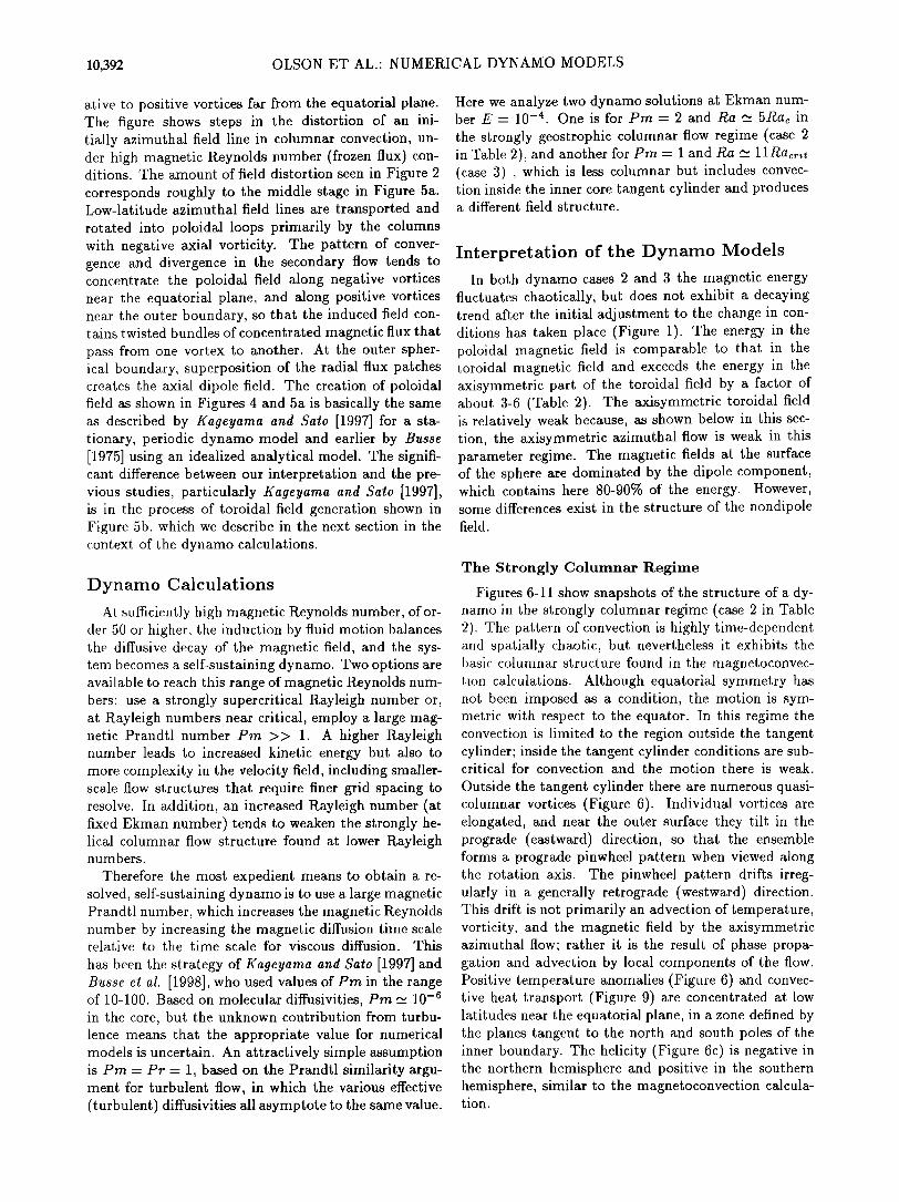
Figure 5a. Schematic illustration of the generation of poloidal field from initial toroidal field by columnar convection. Small arrows indicate the primary (columnar) flow and larger arrows indicate the secondary circulation along the column axes and between columns.

not depend too strongly on the specific boundary conditions. This, in turn, implies that the pattern of helicity negative in the north and positive helicity in the south is likely to be present in the fluid outer core, in the region outside the inner core tangent cylinder. Inside the tangent cylinder, the convection has a different structure and the pattern of helicity is significantly different alSO.

The kinematics by which the basic toroidal field is transformed into a poloidal field by the helicity of the columnar convection is illustrated in Figure 5a. A pair of counterrotating convection columns is shown, separated by a downwelling region with radially inward

flow. The intersection of the convection columns with the outer spherical boundary is indicated by the slop- ing top and bottom of the columns and the equator is shown as a symmetry plane. The closed stream- lines indicate the primary columnar (geostrophic) motion. In addition to the columnar motion, there is the secondary (ageostrophic) circulation consisting of motion toward the equator in both hemispheres within columns with positive vorticity and motion away from the equator within columns with negative vorticity. This ageostrophic motion, indicated by open stream- lines, includes transport from positive to negative vortices near the equatorial plane and transport from neg-

Figure 5b. Schematic illustration of the generation of toroidal field from initial poloidal field by columnar convection.


ative to positive vortices far from the equatorial plane. The figure shows steps in the distortion of an initially azimuthal field line in columnar convection, under high magnetic Reynolds number (frozen flux) conditions. The amount of field distortion seen in Figure 2 corresponds roughly to the middle stage in Figure 5a. Low-latitude azimuthal field lines are transported and rotated into poloidal loops primarily by the columns with negative axial vorticity. The pattern of convergence and divergence in the secondary flow tends to concentrate the poloidal field along negative vortices near the equatorial plane, and along positive vortices near the outer boundary, so that the induced field contains twisted bundles of concentrated magnetic flux that pass from one vortex to another. At the outer spherical boundary, superposition of the radial flux patches creates the axial dipole field. The creation of poloidal field as shown in Figures 4 and 5a is basically the same as described by Kageyama and Sato [1997] for a sta- tionary, periodic dynamo model and earlier by Busse [197,5] using an idealized analytical model. The signifi- cant difference between our interpretation and the previous studies, particularly Kageyama and Sato [1997], is in the process of toroidal field generation shown in Figure 5b, which we describe in the next section in the context of the dynamo calculations.

Dynamo Calculations

At. sufficiently high magnetic Reynolds number, of order 50 or higher, the induction by fluid motion balances the diffusive decay of the magnetic field, and the system becomes a self-sustaining dynamo. Two options are available to reach this range of magnetic Reynolds numbers: use a strongly supercritical Rayleigh number or, at Rayleigh numbers near critical, employ a large magnetic Prandtl number Pm >> 1. A higher Rayleigh number leads to increased kinetic energy but also to more complexity in the velocity field, including smaller- scale flow structures that require finer grid spacing to resolve. In addition, an increased Rayleigh number (at fixed Ekman number) tends to weaken the strongly helical columnar flow structure found at lower Rayleigh numbers.

Therefore the most expedient means to obtain a resolved, self-sustaining dynamo is to use a large magnetic Prandtl number, which increases the magnetic Reynolds number by increasing the magnetic diffusion time scale relative to the time scale for viscous diffusion. This

has been the strategy of Kageyama and $ato [1997] and Busse et al. [1998], who used values of Pm in the range of 10-100. Based on molecular diffusivities, Pm •_ 10 -6 in the core, but the unknown contribution from turbulence means that the appropriate value for numerical models is uncertain. An attractively simple assumption is Pm= Pr = 1, based on the Prandtl similarity argu- ment for turbulent flow, in which the various effective (turbulent) diffusivities all asymptote to the same value.

Here we analyze two dynamo solutions at Ekman number E= 10 -4 One is for Pro= 2 and Ra •_ 5Rac in

the strongly geostrophic columnar flow regime (case 2 in Table 2), and another for Pm= 1 and Ra _• 11Rac,.it (case 3) , which is less columnar but includes convection inside the inner core tangent cylinder and produces a different field structure.

Interpretation of the Dynamo Models In both dynamo cases 2 and 3 the magnetic energy

fluctuates chaotically, but does not exhibit a decaying trend after the initial adjustment to the change in con- dit. ions has taken place (Figure 1). The energy in the poloidal magnetic field is comparable to that in the toroidal magnetic field and exceeds the energy in the axisymmetric part of the toroidal field by a factor of about 3-6 (Table 2). The axisymmetric toroidal field is relatively weak because, as shown below in this section, the axisymmetric azimuthal flow is weak in this parameter regime. The magnetic fields at the surface of the sphere are dominated by the dipole component, which contains here 80-90% of the energy. However, some differences exist in the structure of the nondipole field.

The Strongly Columnar Regime

Figures 6-11 show snapshots of the structure of a dynamo in the strongly columnar regime (case 2 in Table 2). The pattern of convection is highly time-dependent and spatially chaotic, but nevertheless it exhibits the basic columnar structure found in the magnetoconvection calculations. Although equatorial symmetry has not. been imposed as a condition, the motion is sym- metric with respect to the equator. In this regime the convection is limited to the region outside the tangent cylinder; inside the tangent cylinder conditions are subcritical for convection and the motion there is weak.

Outside the tangent cylinder there are numerous quasi- columnar vortices (Figure 6). Individual vortices are elongated, and near the outer surface they tilt in the prograde (eastward) direction, so that the ensemble forms a prograde pinwheel pattern when viewed along the rotation axis. The pinwheel pattern drifts irregularly in a generally retrograde (westward) direction. This drift is not primarily an advection of temperature, vorticity, and the magnetic field by the axisymmetric azimuthal flow; rather it is the result of phase propagation and advection by local components of the flow. Positive temperature anomalies (Figure 6) and convective heat transport (Figure 9) are concentrated at low latitudes near the equatorial plane, in a zone defined by the planes tangent to the north and south poles of the inner boundary. The helicity (Figure 6c) is negative in the northern hemisphere and positive in the southern hemisphere, similar to the magnetoconvection calculation.


TEMPERATURE PERTURBATION VORTICITY

HELICITY FIELD UNES

•'igure 6. Images of temperature perturbations, axial vor[ici[y, helici[y and magnetic field lines (polar view) in 1;he sl;rongly columnar dynamo regime (case 2, Table 2). Lighl; shading, positive; dark shading, negative. Shown are the following surfaces (relative to the maximum value of the variable): T • = +0.3, (V x u): = +0.•, H = +0.4•.

HEAT FLOW RADIAL VELOCITY

RADIAL FIELD

ß HELICITY

•'igure 7. Contours of radial velocity and helici[y at radius r = 0.905 and heat flow and radial magnetic field at the outer boundary in the strongly columnar dynamo regime (case 2, Table 2). Contour intervals are •;u• - 3.18, •;H - 20,400, and •;B• - 0.0508 in units of Table 1.

The map views in Figure 7 reveal that in detail the dipolar field at the surface is formed by superposition of several highly concentrated flux patches that emerge from the fluid at middle and high latitudes in each hemisphere. The flux patches are closely associated with strong, helicity-containing vortices that impinge the outer boundary. As shown previously [Christensen ½t al., lgg8], the flux concentrations correlate strongly with radially inward flow below the surface. In an equatorial crosssection of the sphere, the z component of the field, which represents a large-scale poloidal field, is clearly concentrated into columns with negative vor[ic- ity (Figure 11). The secondary flow along the column axis is directed away from the equator in negative vortices. Therefore the flow must converge toward a negative vortex in the equatorial plane and, [o the extent that the frozen flux approximation is applicable, collect the poloidal field lines. In contrast, at the upper and lower ends of the convection columns at high latitude on the surface, both horizontal flow convergence and magnetic field concentrations are connected [o positive vortices.

The azimuthal averages shown in Figure 10 verify the role of helicity in producing the large-scale poloidal field. The top left image shows the azimuthal average of the product of helici[y and azimuthal field, and represents the axisymmetric c• effect for poloidal field generation, according to mean-field electrodynamic theory


VELOCITY

2O

10

LU

-lO

-2o

0 20 40 60 80

LONGITUDE

MAGNETIC FIELD

x • x.• .... / / .' •.• .' : • X x• '.' ' --

--... --... j, /.. . ,, .. , , • •--. , ß ,

.... ...' ........... . ..... ;•: ........ • . . .. ......... .- •

:' .;' •. •'•'•• •• • • • . • ..' .....•...:

• ' ' '..' :-:.•.. r. .•: .• • • • • •'•.7 '"•. •/' :' ..' .• •///•••• • - '.."..'½'..5 .•: 5.•.w..:: - • ...... •.. :. ' "'-"- ..... ..'v :."q.½//.•.½'• •, 7

•"" .".'?.•'• /././ :' ' '..• .... .:.':'.:..:.."":..:":.":"• •/./ d":. .• ' •'4 • • • , • ..: ..' ..' 5 ,/ .•.• •.. , ..., , • , , ......:' ... ,• •. .• 5. • .., , ', •...• •

0 20 40 60 80

LONGITUDE

Figure 8. Detail of the magnetic and velocity fields from the maps shown in Figure 7. Contour intervals for radial velocity and radial magnetic field are •ur - 3.18; •Br - 0.087. Vectors show the horizontal velocity and magnetic fields.

[Moffatt, 1978]. The azimuthal field represents largely the toroidal field component, and in this case the helicity is formed only from the radial and latitudinal components of velocity and vorticity because only that fraction of heliciW can act on the azimuthal magnetic field. This product correlates closely with the distribution of the axisymmetric toroidal current, which generates the poloidal field, outside the inner core tangent cylinder (Figure 10). As in the magnetoconvection case, an a effect proportional to helicity in the columnar convection is the source of the axisymmetric poloidal field. The detailed structure of the poloidal field can be explained by the concentration and dispersal of the large-scale magnetic field by local flow convergence and divergence, respectively.

We now turn to the mechanism for toroidal field generation. In many dynamo models the toroidal field is maintained by variations in the axisymmetric angular velocity interacting with the main poloidal field, through the • effect [Parker, 1955; Holierbach, 1996]. For example, thermal wind within the tangent cylinder

provides an • effect for toroidal field generation in the Glatzmaier and Roberts [1995a] dynamo model. These flows have been proposed as driving mechanism for inner core super-rotation [Glatzmaier and Roberts, 1996; Aurnou et al., 1996]. In the Kuang and Bloc:ham [1997] dynamo model, an • effect due to large-scale azimuthal flow outside the tangent cylinder leads to strong toroidal fields in that region.

There are axisymmetric variations in angular velocity in our calculations, which produce toroidal field through the • effect. However they are not the main source of toroidal field for dynamos dominated by strongly columnar convection. Figure 10 demonstrates this point. The upper right and lower right images show contours of the axisymmetric azimuthal field intensity and the • effect, respectively. The • effect image shows the azimuthal average of rB•O(r-•u•)/Or+r-•sinOBo O(sinO-•u• from the azimuthal component of the magnetic induction equation. Positive correlation between these two images indicates places where the • effect generates imuthal field. There are some localized regions of corre-


KINETIC AND MAGNETIC ENERGY

...... :,:::?:'". ',?:;..- .......... :

:•':;" .... ii:.•:'.';•;• "':':•" r- ::•.

--:• "'::•i•-;,;;-*:t:':;:"'--':.. '•

*•m .... ''. ....... '"':' % :• :..'• .•..--..:; ........

---• ,,..., :;•..:. ., .....

ADVECTED HEAT •. ..-- ..•.-•-•• ....

,.•.......•: •:• •:• •-?•..;,; ..... i• ...... '"'"'>• ....

..• •'•"-½. '•,'.••-•.:.....:.•:,x½•...--½i•.. .---:•*;.:•'""%,,.,;•,:--•½•.•

.•: •,%,.•:-:½-•?• ,<•'-'.::::•-;•!:•. -:.; •:•:'•:•::½.• -

:a* ....... ::::.:.-':-'-----, :: ........... •... -.. .::::.:..• ....... :::::; :;.:-:-::: .......

':'•'•m"?'::':::•:½.:::;; ......... ';;;:'a;i""*:;:*-•'•' '":'":"':**•**:•' ' -:.-• ....... .:•.: .......... .:, .... .....>. :?- . ....................... . ......... ::,:.:.'•""•:.•

"•. :•,:-.• :-•:.:i,• .......... •,:•-..' .... •:'• .;.4 •

.... -......-.-..-.-...- ..• .

JOULE HEAT WORK AGAINST LORENTZ FORCE

..... ,,, :::::::::::::::::::::::::::::::::::::::::::::::::::::::::::::

. ,.:. '-•-'-'--•:• Figure 9. Images of kinetic and magnetic energy density, advected heat, Joule heating and work done against the Lorentz force in the strongly columnar dynamo regime (case 2, Table 2). Light shading, kinetic energy; dark shading, magnetic energy. Shown are the surfaces (relative to the maximum value of the variable): E•,: 0.5, E•: 0.3, W•,, W•, ß = 0.2.

-HELICITY x Bphi AZIMUTHAL FIELD

AZIMUTHAL CURRENT MEAN OMEGA

lation between these two images, particularly within the tangent cylinder. However, outside the tangent cylinder, where the azimuthal field is concentrated, the • effect and the azimuthal field are negatively correlated. Here the • effect opposes the main azimuthal field, and so cannot be the primary mechanism for generating it.

In order [o understand the generation mechanism, we must consider the detailed structure of the toroidal

field. From Figure 10 its axisymmetric part is strongly

Figure 10. Contours of the axisymmetric structure in the strongly columnar dynamo regime (case 2). These images help diagnose the origin of the poloidal and toroidal magnetic fields. The upper left image is the product of helicity and azimuthal field, the c• effect source of toroidal current and poloidal magnetic field. It correlates with the calculated azimuthal currents (lower left) outside the inner core tangent cylinder. The axisymmetric poloidal field lines are superimposed on the currents. The lower right image is the w effect source of toroidal magnetic field. It correlates with the calculated azimuthal magnetic field (upper right) inside the inner core tangent cylinder, but not outside. Contour intervals are 5J• k = 1.23, 5(HB•k) = 2840, 5B• k = 0.211 in the units of Table 1, and 5w = 23 .


TEMPERATURE

Z-VORTICITY Z-FIELD

Figure 11. Equatorial plane section of case 2. Shown are contours of temperature (upper left), z component of the magnetic field (upper right), z component of vorticity (lower left), and the z derivative of the in-plane component of the magnetic field. Because the field is antisymmetric with respect of the equator, the arrows can also be taken as a representation of the field at a short distance north of the equatorial plane. Contour intervals are 5T = 0.0625, 5B, = 0.24, •w: 509.

concentrated into bundles of opposing polarity at low latitudes on either side of the equatorial plane and is most intense near the outer surface. A close-up image of this region (Figure 8) reveals that intense toroidal field bundles occur in separated segments that bend around the convection columns. An individual bundle in the

northern hemisphere originates at a middle latitude radial flux patch correlated with intense downwelling and connects to a radial flux spot of inverse polarity at low latitude, which is often located at the edge between upwelling and downwelling regions. As the magnetic field is antisymmetric about the equator, the inverse spots occur in pairs. While in this case only weak traces of the inverse radial field penetrate to the surface (Figure 7), more pronounced inverse spots can be observed in other model calculations [Christensen et al., 1998]. The segmented structure of the toroidal field bundles can also be seen in the equatorial section in Figure 11. Cor- relating the horizontal field with the thermal structure shows that the toroidal field bundles are most intense

above broad warm plumes and turn into low-latitude, inward directed radial fields in the cold downwellings.

The detailed structure of the low-latitude toroidal

field bundles suggests that it is created and intensi- fied by the columnar convection itself, through the same macroscopic c• effect mechanism that creates the poloidal field. The kinematics of toroidal field generation in these dynamos is illustrated schematically in Figure 5b, which depicts in stages the conversion of poloidal to toroidal magnetic fields by columnar flow. The process can be visualized by considering the evolution in time of an initially straight poloidal field line located in an upwelling between two columnar vortices. Using the concept of frozen flux, the field line is advected toward the observer while simultaneously be- coming twisted by the secondary flow. After roughly one-half rotation of the primary circulation, the field line has been transported to the front of the vortices by the primary flow and rotated by the secondary flow into an inclined azimuthal orientation. Because a material

line of fluid moving toward the observer must shorten along the z direction, there is an additional component of convergent flow toward the equatorial plane in an upwelling (which is independent from the secondary,


10 4

• 0 3 el

i i i I

0.2 0.4 0.6 0.8 1 Time

Figure 12. Time series of magnetic and kinetic energy for a calculation with Ra = 418 and otherwise same

parameters as case 2, starting at a time where the magnetic field intensity is artificially decreased. Time is scaled by magnetic diffusion time.

helicity-producing circulation). This flow component advects the azimuthally oriented portion of the field line toward low latitude. As the field line approaches the front of the columns, its azimuthal component is stretched by the divergence in the azimutha,1 motion locally enhancing this component of the field and producing the intense flux bundles at low latitudes. The final field line structure at low latitudes in configuration to the right in Figure 5b is remarkably similar the structure of the field seen in the calculations. Note

that the final field line configurations in Figures $a and $b are similar when phase shifted so that the flow pat- terns match. This indicates that the same equilibrium field line configuration can be reached starting with either a purely axial (poloidal) field or with a purely imuthal (toroidal) field. The result is an equilibrium dynamo of the c• 2 type, which contains similar energy in the poloidal field as the toroidal field. Large-scale azimuthal flows play little or no role in this regime. In comparison with previous dynamo models, our numerical results are most similar to the asymptotic model of Busse [1975].

Next we address the question of the field equilibration mechanism. Figure 9 shows the 3-D distribution of kinetic and magnetic energy densities E• and Era, Joule heating •, and the work done on the fluid by buoyancy and Lorentz forces, W• and Wœ. Comparison with Fig- ure 6 shows that the kinetic energy is concentrated near the negative vortices, while the magnetic energy concentrates in regions with lower kinetic energy, particularly at low latitudes. The rough anticorrelation of kinetic and magnetic energy can be interpreted in two ways. It can be partly explained by the well-known tendency for the magnetic flux to be expelled from regions where the magnetic l:Leynolds number is high and where the circu-

lation is closed [Moffatt, 1978]. However, it could also indicate that in regions of strong magnetic field the associated Lorentz forces locally reduce the flow velocity. This suggests that the equilibration of the dynamo is simply a reduction of the vigor of convection in strong magnetic fields.

Additional support for the interpretation that equilibrium is maintained locally on each column comes from the similarity in the distributions of Wb and Wœ, and ß shown in Figure 9. According to (14), in a convection-powered dynamo it is sufficient for these t. erms to balance in a global, time-averaged sense only. But. W•, W•, and ß are all of the same order, and all vary on the scale of the columns, directly related to the kinematics of the columnar flow (as illustrated in Fig- ures $a and $b). Furthermore, the fact that these terms have nearly the same spatial distribution over time implies that, for this dynamo, a local energy balance is involving these terms is maintained at each moment in time.

The reduction in the vigor of the columnar convection through the Lorentz force is demonstrated in a calcula.t, ion where we reduce the magnetic field intensity everywhere by multiplying the instan•.aneous field by the factor 0.02 in a fully developed (strong-field) dynamo case and then continue the calculation. The Lorentz

forces are thus reduced by a factor of 2500 and should have negligible influence. We find that the original field intensity is recovered within 2.5 dipole diffusion times, showing tha; non-magnetic convection is probably un- stable against magnetic perturbations at these parameter values. The experiment was done at a somewhat higher Rayleigh number than we employed in case 2, but a similar experiment at a lower Rayleigh number yielded a similar result, suggesting that the same holds for the case discussed here. Upon reduction of the field intensity, the kinetic energy nearly doubles in a rapid adjustment and stays at the high level as long as the magnetic field remains comparatively weak (Figure 12). However, once the field intensity approaches a value corresponding to an Elsasset number of 1, the kinetic energy drops and the field growth slows. Eventually, when the full field strength is recovered, the time-averaged kinetic energy is reduced to 60% of its value during the weak-field stage.

As the field intensity began to recover, there was no substantial change in the overall pattern of the convection, apart from the decreases in energy already noted. Neither was there a substantial change in the pattern of the secondary axisymmetric azimuthal flow, or its kinetic energy relative to the total kinetic energy. The basic kinematic elements of these dynamos, including the o• effect from helicity in the columnar convection and the anti-co effect from the mean azimuthal flow , are present both far and near equilibrium conditions, in roughly the same proportions.

We wish to draw particular attention to these aspects of the recovery tests, because they have a special bear-


RADIAL FIELD AT t= 0.456 AZIMUTHAL VELOCITY

RADIAL FIELD AT t= 0.464 CROSS CORRELATION & TRANSPORT

Figure 13. Contours of radial magnetic field on the outer boundary at the times indicated, azimuthal velocity during the time interval, and the cross correlation of the radial field at the two times, for case 2. The thin curve on the cross-correlation diagram is the transport (displacement) implied by the axisymmetric azimuthal flow during the time interval.

ing on the question of how these dynamos equilibrate. According to the Malkus-Proctor [1975] mechanism, azimuthal flows driven by Lorentz forces create an anti-• effect, by inducing fields that oppose the field induced by the convection. Although we indeed observe an anti- • effect in these calculations, the recovery tests indicate it is not the important equilibration mechanism here, since it, is present in basically the same form at all field strengths. Instead it appears to be largely a secondary flow driven by mechanical forces and is of secondary importance for both field generation and equilibration in this parameter range. It would be interesting to determine whether the column-by-column equilibration mechanism we have identified in these calculations

persists for different parameters, particularly at lower Ekman numbers.

Finally, we consider time variations of the magnetic field on the outer boundary, specifically the azimuthal drift of the nondipole field. Figure 13 shows two snapshots of the radial field structure on the outer bound-

ary separated by 0.01 time units, the cross correlation between the two, and the pattern of azimuthal velocity at r=0.94 during this time interval. The dashed curve superimposed on the cross correlation shows the amount of displacement (transport) by the axisymmetric azimuthal flow during the time interval. The cross correlation demonstrates that the drift direction is gen-

erally retrograde (westward), particularly at low latitudes. The displacement by the axisymmetric flow is everywhere smaller and in many places opposed to the drift direction. In addition, the pattern of azimuthal flow does not correlate with the pattern of drift de- duced from the cross correlation. This means that the

westward drift is generally not the result of advection of the field by the fluid motion. Instead, most of the coherent westward drift comes from the rapid, episodic phase propagation of the patches of reversed flux at low latitudes, as can be seen in the radial field images in Figure 13. This could be a wave phenomenon involving both the field and the flow, or it could be a kinematic effect due to time variations in the pattern of horizontal divergence and convergence of north-south flow.

The Fully Developed Regime

For a fixed Ekman number, as the Rayleigh number increases, convection is excited inside the tangent cylinder. We refer to this regime as fully developed convection, to distinguish it from the previous case in which t. he tangent cylinder regions are subcritical with respect to convection. Plates 1,2 and Figures 14,15 show the results for a dynamo driven by fully developed convection. The parameters of this case are summarized as case 3 in Table 2.

Because the buoyancy forces are larger relative to Coriolis forces in the fully developed regime, the fluid motion is more three-dimensional and has become asym- metric with respect to the equator compared to the highly columnar regime. This is evident by comparing the images in Plates 1-2 and Figures 14-15 with their counterparts from the previous case. The temperature perturbations in Plate i show greater departure from azimuthal periodicity and equatorial symmetry than the previous case. In addition, there is a large positive temperature perturbation inside the tangent cylinder, indicating the presence of a hot plume upwelling along the rotation axis at the poles. The vorticity shown in Plate i is still elongated parallel to the spin axis, but the vortices are more truncated and wavy than in the strongly columnar regime.

As shown in Figure 14, the large-scale field is again dominated by the axial dipole component, which is formed by the superposition of several bundles of concentrated radial flux at the outer boundary, as shown in Plate 2. In this case the bundles at high latitudes are more prominent, arrayed around the intersection of the inner core tangent cylinder with the outer boundary. Some of the flux bundles and the low-latitude patches of reversed flux exhibit episodes of retrograde drift, and as in the previous case this appears to be more of a propagation effect than advection of the field by the azimuthal fluid motion. To illustrate this point, Figure 14 shows the axisymmetric azimuthal velocity. Outside the tangent cylinder, the azimuthal velocity is generally small and its sign varies near the outer boundary, and so cannot be the main cause of the more uniform retro-

OLSON ET AL.- NUMERICAL DYNAMO MODELS 10,399

TEMPERATURE PERTURBATION VORTICITY

ANGULAR VELOCITY FIELD LINES

Plate 1. Images of temperature perturbations, z vorticity, angular velocity perturbations and field lines (polar view) in the fully developed convection dynamo regime (case 3, Table 2). Red/yellow, positive; blue, negative. Shown are the following surfaces (relative to the maximum value of the variable): T' = 4-0.3, (U' x u)z = 4-0.35.

10,400 OLSON ET AL.- NUMERICAL DYNAMO MODELS

HEAT FLOW RADIAL VELOGITY

RADIAL FIELD HELICITY

Plate 2. Contours of radial velocity and helicity at radius r - 0 922 and heat flow and radial magnetic field at the outer boundary in the fully developed convection dynamo regime (case 3, Table 2). Contour intervals are 5u? - 17.2, 5H - 133,000, and 5B? - 0.19 in units of Table 1.


VELOCITY AZIMUTHAL FIELD

AZIMUTHAL CURRENT MEAN OMEGA

Figure 14. Contours of azimuthal averages in the fully developed convection dynamo regime (case 3, Table 2). These images help diagnose the origin of the poloide[1 and toroide[1 magnetic fields. The upper left image shows the azimuthal velocity. The lower left shows imuthe[1 currents. The lower right image is the w effect source of the toroidal magnetic field. It correlates with the actual azimuthal magnetic field (upper right) inside the inner core tangent cylinder but generally not outside. Contour intervals are 5J• = 3.3, 5ur) : 13, 5B• = 0.214 in the units of Table 1, and 5w = 80 .

grade drift of the field. Inside the tangent cylinder, the azimuthal velocity is strongly retrograde near the outer boundary and becomes weak or even prograde at the inner core boundary. This represents a thermal wind flow (el be[roclinic vortex surrounding the polar upwelling in which the circulation changes with height) driven by the lateral temperature variations shown in Plate 1.

The map images in Plate 2 confirm the departure from equatorial symmetry when the convection is fully developed. The surface heat flow reveals the prominent plume upwelling along the rotation axis. Greater departure from equatorial symmetry is expected in the fully developed regime, in part because the geostrophic constraint is weaker, but also because the motion inside the tangent cylinders above and below the inner core are geometrically isolated from each other, and are therefore free to evolve independently.

The correlation between the product of helicity and azimuthal field with the azimuthal current distribution

(not shown) confirms that the poloidal field outside the

tangent cylinder is mostly generated by an c• effect similar to case 2. But within the tangent cylinder the toroide[1 currents have their source in the mean merid-

ionell circulation connected to the polar upwelling (Fig- ure 14). This circulation advects the poloidal field lines toward the rotation axis near the inner boundary ri and away from the rotation axis near the outer boundary to, producing eastward totolde[1 currents near ri and westward toroide[1 currents near to, in each hemisphere. This represents a modification of the poloide[1 field by meridione[1 flow, the m effect in mean-field dynamo theory [Roberts, 1972]. These currents distort the poloide[1 field lines within the tangent cylinder, enhancing the poloide[1 field near ri and reducing it near to, relative to a simple dipole field.

Advection of the poloide[1 field by the polar upwelling partly explains the pattern of radial field intensity variations at high latitudes on the outer boundary, shown in Plate 2. There is e[ deep local minimum in the field strength at the pole, directly above the upwelling. The calculated w effect outside the tangent cylinder is generally anticorrelated with the axisymmetric azimuthal field (Figure 14) suggesting an c• effect mechanism for the generation of that part of the toroide[1 field, as es- tablished in case 2. However, for the intense toroide[1 flux bundles inside the tangent cylinder the correlation is positive, and their origin can be understand in terms of the shearing effect of the gradient of the thermal wind

HEAT FLOW RADIAL VELOCITY

:C

Figure 15. Contours of radial velocity and helicity in the Ekman 1Wet at radius r = 0.3596 and heat flow and radial magnetic field at the inner boundary ri = 0.3506 in the fully developed convection dynamo regime (c•e 3, Table 2). Contour intervals are 5u• = 3.56, 5H = 47,742, and 5B, = 0.661 in the units of Table 1.


along the z axis and the z component of the dipole field in that region.

Summary and Implications for the Geodynamo

Thermal convection in e[ rotating spherical shell is a highly effective dynamo mechanism. The convection adopts a quasi-columnar planform with secondary flow up the columns with negative vorticity and down the columns with positive vorticity. This results in negative hellcity in the northern hemisphere and positive helicity in the southern hemisphere, which efficiently converts a toroidal to a poloidal magnetic field. Con- version of the poloidal to toroidal field outside the inner core tangent, cylinder is also accomplished by the helicity of the columnar flow. We have identified two regimes for dynamo action, based on the presence of convection inside the inner core tangent cylinder. In the strongly columnar regime the tangent cylinder is subcritical with respect to convection, large-scale azimuthal flow is weak and the magnetic field is generated by an c• • mechanism in the columns. At high magnetic Reynolds number in this regime, the field is concentrated in flux bundles that wrap around the convection columns.

Convergence and divergence of the columnar and secondary flow concentrates the poloidal field into negative vortices in the equatorial plane and into radial downwellings at the outer surface, and at high latitude, cor- respond to the ends of positive vortices. Superposition of several flux bundles results in a strong axial dipolar field. The average azimuthal field results from superposition of the twisted portions of the flux bundles and is similar in strength to the axial dipole field. This energy partitioning between field components is different from other dynamo models [Kuang and Blozham, 1997; Glatzma,½r and Roberts, 1995a] and differs from the generally accepted view about the core, where it is often assumed that the toroidal field is much stronger than the poloidal field [Holierbach, 1996] due to an w effect. Equilibrium in our dynamos is maintained locally on each convection column, through an approximate equality of the work done by buoyancy forces and work done against the Lorentz force, which reduces the vigor of the flow. The nondipole field at the outer boundary exhibits episodes of westward drift, mainly due to retrograde azimuthal phase propagation of low latitude patches of reversed flux. In terms of the classification used in mean-field electrodynamics, these dynamos are of the c• • type, and the mechanisms involved are very similar to the asymptotic model of Busse [1975].

A second dynamo regime occurs in calculations at higher Rayleigh number (for fixed Ekman number) and is characterized by fully developed flow inside and outside the tangent cylinder, and less symmetry with respect to the equatorial plane than in the highly columnar regime. Our dynamo calculations in this regime contain elements of similarity with the Glatzmaier and

Roberts dynamos, which were made at proportionally lower Ekman number and higher Rayleigh number. In this regime there are polar upwellings and thermal wind azimuthal flows inside the tangent cylinder. Outside the tangent cylinder, the convection consists of vortices aligned with the spin axis, although the vortices are less coherent than in the columnar regime. As in the columnar regime, poloidal magnetic flux bundles form on the outer boundary, but in the fully developed regime they are more prominent at the latitude where the inner core tangent, cylinder intersects the outer boundary. The polar upwellings create a local minimum in field intensity on the outer boundary at the pole. The drift direction is again dominantly retrograde (westward), although it is highly episodic and irregular. It cannot be explained by advection by the axisymmetric azimuthal flow and instead appears to be a phase propagation effect. The toroidal field is generated in part by the columnar convection outside the tangent cylinder and partly by an c• effect due to interaction of the large-scale poloidal field with the thermal wind inside the tangent cylinder. In terms of the mean-field theory classification these dynamos are similar to the c•2a; type. The dynamo at E - 3 x 10 -4 Pm- 2 and 6Rac described by Christensen ½t al. [1998] belongs in this category. A comparison with case 3 presented here suggests that it requires, at lower Ekman number, a higher supercritical Rayleigh number to reach the fully developed regime.

All of the dynamos presented here are simplified in many ways relative to conditions in Earth's core, and consequently, any interpretation of the results in terms of processes affecting the geodynamo is uncertain. How- ever, there are some general results that may apply to the core in a qualitative sense. First, the tendency for the poloidal field to become concentrated into bundles has obvious implications for interpreting the structure of the geomagnetic field in terms of the pattern of core convection. The geomagnetic field on the core-mantle boundary is concentrated in two high-latitude flux bundles in each of the northern and the southern hemi-

spheres, located at approximately the latitude of the inner core tangent cylinder and at approximately the same longitudes in the two hemispheres, as shown in the field models of Bloc:ham, et al. [1989]. Gubbins and Bloz'ham [1987] have interpreted these structures as indicating convection columns in the fluid outer core po- sitioned near the inner core tangent cylinder. As seen in Figure 7 and Plates 1 and 2, our calculations also contain high latitude flux bundles, although more than just two in each hemisphere. This difference could be due to smoothing in the geomagnetic field models.

Other features of the geomagnetic field that may be equally important for interpreting the geodynamo are the polar minima in field intensity. Unlike a pure axial dipole, the core field has a relative minimum near the pole in both hemispheres, and even reversed flux at the north pole [Bloc:ham and Jackson, 1992]. As Fig- ures 7 and Plate 2 show, our dynamo models also have


local minima in field intensity on the outer boundary near each pole, particularly the calculations in the fully developed convective regime. On the basis of other dynamo calculations, we previously suggested that the polar field intensity minima indicate convective upwellings in the outer core along the rotation axis in each hemisphere [Christensen et al., 1998]. Figure 14 shows that upwelling and the accompanying thermal wind vortex flow in the fully developed regime.

This interpretation bears on the cause of the seismically inferred superrotation of the solid inner core [Song and Richards, 1996; $uet al., 1996; Creager, 1997]. Dynamo models achieve superrotation through electromagnetic coupling between the thermal wind inside the tangent cylinder and the electrically conducting inner core [Glatzmaier and Roberts, 1996]. Since the upwelling accompanies the polar thermal wind vortex, inner core superrotation and polar flux minima are phe- nomena related to one another by the structure of the convection. Thus it would be of great interest to fur- ther resolve the structure and secular variation of the

geomagnetic field in polar regions of the core-mantle boundary, to determine if there is additional evidence for this style of convection.

Figure 15 shows map views of the heat flow and radial field on the inner boundary, plus radial velocity and helicity a short radial distance away, near the top of the Ekman layer, in the fully developed convection case. Note the single bundle of radial field on the pole, concentrated there by convergence toward the polar upwelling. Also the helicity is reversed in the Ekman layer, compared to the distribution in the fluid interior shown in Plate 2. In addition, Figure 15 shows the heat flow on the inner boundary is strongly concentrated at low latitudes and correlates inversely with the pattern of radial velocity in the columnar convection. On the inner boundary the azimuthally averaged heat flow is about 7 times higher on the equator than at the poles. This pattern has implications for the way in which the inner core crystallizes and possibly for the development of inner core anisotropy. Yoshida et al. [1996] and Bergman [1997] have argued that preferred crystallization at the inner core boundary equator (rather than uniform crystallization over the whole boundary) is critical for ex- plaining the seismically observed pattern of inner core anisotropy. Although our calculations do not include inner core crystallization explicitly (or anomalous inner core rotation, for that matter), they indicate that a columnar convection dynamo preferentially extracts heat from the inner core equator, resulting in enhanced crystallization in that region.

Another group of structural features that were previously noted in dynamo models by Christensen e! al. [1998] and which also appear in these dynamos are the reversed flux spots at low latitudes (see Plate 2). Low- latitude reversed flux spots are prominent on the core- mantle boundary. Blozharn [1986] has interpreted these in terms of the expulsion of mainly toroidal flux by

convective upwellings. The results of our calculations basically conform to this interpretation, although we find that individual reversed flux spots can be formed at several different locations by the columnar convection, including upwellings and at the margins of certain downwellings. But in every case the expelled flux orig- inated from the toroidal field, and the location of the

spots indicates the sites where the stretching of the field lines by the columnar convection is most intense.

In the parameter regime we have investigated, dynamo action occurs by an c• effect generating both the poloidal and the toroidal field. The c• effect is de- rived primarily from helicity in the columnar convection. Equilibrium between magnetic and kinetic energy, and the equilibration between sources and sinks of magnetic and kinetic energy are maintained locally, on the scale of individual columns. Our calculations differ in

these attributes from some other dynamo models, in which large-scale azimuthal flows play a critical role, both in field generation and equilibration.

In spite of this fundamental difference, the structure of the magnetic fields produced by dynamos in the regimes we have investigated are rather similar to other recent dynamo models. This similarity seems to be the result of the basic ingredients common to all such models: the spherical shell geometry and the control of the convection by a combination of Coriolis, buoyancy and Lorentz forces.

Acknowledgments. This work has been supported by the Los Alamos IGPP, by the NASA HPCC program, and by the Deutsche Forschungsgemeinschaft.

References

Aurnou, J.M., D. Brito, and P.L. Olson, Mechanics of inner core super-rotation, Geophys. Res. Lctt., 23, 3401-3404, 1996.

Bergman, M.I., Measurements of elastic anisotropy due to solidification texturing and the implications for the Earth's inner core, Nature, 389, 60-63, 1997.

Busse, F.H., Thermal instabilities in rapidly rotating systems, J. Fluid Mech., 44,, 441-460, 1970.

Busse, F.H., A model of the geodynamo, Geophys. J. R. Astron. Soc., 4,2, 437-459, 1975.

Busse, F.H., E. Grote and A. Tilgner, On convection driven dynamos in rotating spherical shells, Stud. Geophys. Geod., 42, 1-6, 1998.

Bloxham, J., The expulsion of magnetic flux from the Earth's core, Geophys. J. R. Astro. Soc., 87, 669-678, 1986.

Bloxham, J., D. Gubbins and A. Jackson, Geomagnetic secular variation, Phil. Trans. Roy. Soc. London Set. A, 329, 415-502, 1989.

Bloxham, J., and A. Jackson, 1992, Time-dependent mapping of the geomagnetic field at the core-mantle boundary, J. Geophys. Res., 97, 19357-19564, 1992.

Cardin, P., and P. Olson, The influence of toroidal mag-


netic field on thermal convection in the core, Earth Planet Sci. Lett., 1S2, 167-181, 1995.

Christensen, U., P. Olson, and G.A. Glatzmaier, A dynamo model interpretation of geomagnetic field structures, Geophys. Res. Lett., 25, 1565-1568, 1998.

Creager, K.C., Inner core rotation rate from small-scale heterogeneity and time-varying travel times, Science, 287, 1284-1288, 1997.

Fearn, D.R., Hydromagnetic flow in planetary cores, Rep. Prog. Phys., 61, 175-235, 1998.

Fearn, D.R., M.R.E. Proctor and C.C. Sellar, Nonlinear magnetoconvection in a rapidly rotating sphere and Taylor's constraint, Geophys. Astrophys. Fluid Dyn., 77, 111-132, 1994.

Gilman, P.A. and J.Miller, Dynamically consister • nonlinear dynamos driven by convection in a orating spherical shell, Astrophys. J. Suppl., 46, 211-236, 1981.

Glatzmaier, G.A., Numerical simulations of stellar convective dynamos. I. The model and method, J. Corn- put. Phys., 55, 461-484, 1984.

Glatzmaier, G.A., and P.H. Roberts, A three-dimensional convective dynamo solution with rotating and finitely conducting inner core and mantle, Phys. Earth Planet. Inter., 91, 63-75, 1995a.

Glatzmaier, G.A., and P.H. Roberts, A three-dimensional self- consistent computer simulation of a geomagnetic reversal, Nature, 377, 203-208, 1995b.

Glatzmaier, G.A., and P.H. Roberts, Rotation and mag- netism of Earth's inner core, Science, 27•, 1887-1891, 1996.

Glatzmaier, G.A., and P.H. Roberts, Simulating the geodynamo, Contemporary Phys., 38, 269-288, 1997.

Gubbins, D., and J. Bloxham, Morphology of the geomagnetic field and implications for the geodynamo, Nature, 325, 509-511, 1987.

Holierbach, R., On the theory of the geodynamo, Phys. Earth Planet. Inter., 98, 163-185, 1996.

Holierbach, R., and C.A. Jones, A geodynamo model incorporating a finitely conducting inner core, Phys. Earth Planet. Inter., 75, 317-327, 1995.

Jones, C.A., A.W. Longbottom, and R. Holierbach, A self-consistent convection driven geodynamo model using a mean field approximation, Phys. Earth Planet. Inter., 92, 119-141, 1995.

Kageyama, A., and T. Sato, Generation mechanism of a dipole field by a magnetohydrodynamical dynamo, Phys. Rev. E, Stat. Phys. Plasmas Fluids Relat. Inter- discip. Top. 4617-4626, 1997.

Kuang, W., and J. Bloxham, An Earth-like numerical dynamo model, Nature, 389, 371-374, 1997.

Malkus, W.V.R., and M.R.E. Proctor, The macrody- namics of a-effect dynamos in rotating fluids, J. Fluid Mech., 67, 417-444, 1975.

Moffatt, H.K., Magnetic Field Generation in Electrically Conducting Fluids, 343pp., Cambridge Univ, Press, New York, 1978.

Olson, P., and G. A. Glatzmaier, Magnetoconvection in a rotating spherical shell: structure of flow in the outer core, Phys. Earth Planet. Inter., 92, 109-118, 1995.

Olson. P., and G. A. Glatzmaier, Magnetoconvection and thermal coupling of the Earth's core and mantle, Philos. Trans. R. Soc. London Set. A, 35•, 1413-1424, 1996.

Parker, E.N., Hydromagnetic dynamo models, A stro- phys. Y., 122, 293-314, 1955.

Roberts, P.H., Kinematic dynamo models, Philos. Trans. Fl. Soc. London Set. A, 272, 663-698, 1972.

Sarson, G.R., C.A. Jones, and A.W. Longbottom, The influence of boundary region heterogeneities on the geodynamo, Phys. Earth Planet. Inter., 101, 13-32, 1997.

Song, X., and P.G. Richards, Seismological evidence for the differential rotation of the Earth's inner core, Na- ture, 382, 221-224, 1996.

Su, W.-J., A.M. Dziewonski, and R. Jeanloz, Planet within a planet: Rotation of the inner core of the Earth, Science, 27d, 1883-1888, 1996.

Walker, M.R., and C.F. Barenghi, Magnetoconvection in a rapidly rotating sphere, Geophys. Astrophys. Fluid Dyn., 85, 129-162, 1996.

Yoshida, S., I. Sumira, and M. Kumazawa, Growth model of the inner core coupled with outer core dy- namics and the resulting elastic anisotropy, J. Geo- phys. Res., 101, 28085-28103, 1996.

Zhang, K-K., Spherical shell rotation convection in the presence of a toroidal magnetic field, Proc. R. Soc. London ,5'er. A, 448, 245-268, 1995.

Zhang, K-K., and D. Gubbins, Convection in a rotating spherical fluid shell with an inhomogeneous temperature boundary condition at infinite Prandtl number

J. Fluid Mech., 250, 209-232, 1993. Zhang, K-K., and C.A. Jones, Convective motions in

the Earth's fluid core, Geophys Res Lett, 21, 1939-1942, 1994.

Zhang, K-K., and C.A. Jones, On small Roberts number magnetoconvection in rapidly rotating systems, Proc. R. $oc. London $er. A, 25d, 981-995, 1996.

Zhang, K-K. ,and C.A. Jones, The effect of hypervis- cosity on geodynamo models, Geophys. Res. Lett., 2869-2872, 1997.

U. Christensen, Institut fiir Geophysik, Universitiit GSttingen, 37075 GSttingen, Germany.

G. Glatzmaier, Earth Sciences Department, University of California, Santa Cruz, CA 95064.

P. Olson, Department of Earth and Planetary Sciences, Johns Hopkins University, Baltimore, MD 21218.

(Received July 28, 1998; revised December 30, 1998; accepted January 7, 1999.)

Numerical modeling of the geodynamo: Mechanisms of field

Documents

Transcript of Numerical modeling of the geodynamo: Mechanisms of field