NUMERICAL MODELING OF BRITTLE ROCK FAILURE UNDER DYNAMIC STRESS LOADING

N. Golchinfar and M. Cai

Laurentian University 935 Ramsey Lake Road

Sudbury, Canada P3E 2C6

NUMERICAL MODELING OF BRITTLE ROCK FAILURE UNDER DYNAMIC STRESS LOADING

ABSTRACT

Tunnels in deep mines are subjected to high stresses. Fracture and failure of the rock mass around an

opening can occur when mining-induced stresses are high. In burst-prone grounds, mining-induced seismicity can cause additional dynamic loading which can further increase the stress around the tunnels. When the dynamic stress reaches the rock mass strength, fracturing can occur and rockburst may happen (depending on loading stiffness around the failed rock mass). Rock support installed in the tunnel must be capable of dissipating dynamic energy and holding the failed rocks. Hence, it is important to estimate the depth of failure for rock support design. This paper focuses on how to model depth of failure under dynamic loading. In the modeling, two scenarios of rock failure are considered. In the first scenario, rock failure occurs under static loading and subsequent dynamic loading further increases the depth of failure. In the second scenario, no failure occurs under static loading but in the subsequent dynamic loading, failure around the tunnel is created.

KEYWORDS

Depth of failure, dynamic loading, tunnel, rockburst, seismicity, rock support, numerical modeling.

INTRODUCTION Under high static stresses, fracture and damage of rock mass around an opening can result from high

mining-induced stresses, leading to brittle rock failure around the excavation boundary. In burst-prone grounds, mining-induced seismicity can cause additional dynamic loading which may further increase the stress around the tunnel, leading to more failure, loosening, sudden release of elastic strain energy stored in the failing rocks and the surrounding rock masses, and violent ejecting of the failed rock masses (Kaiser et al., 1996).

Once the anticipated seismic damage risk is recognized, it is important to control the potential damage caused by the seismic event. First, the demands that will be imposed on the support systems need to be estimated. Then, rock support with sufficient capacity must be designed and installed to control the potential failure zone, to provide a safe environment for the underground workers, and to avoid disruption to mine production. One method to estimate the support capacity under dynamic loading is the energy approach which is based on the estimation of the maximum ejection velocity (Stacey & Ortlepp, 1993). Another method relies on a reasonable estimate of the ultimate depth and extent of the failed rocks under both static and dynamic loadings; to achieve this goal, it is important to anticipate the brittle rock failure zone around the excavation under both static and dynamic loadings.

PURPOSE OF THE STUDY

The depth of failure is an important factor to be considered when designing rock support systems (Cai et

al., 2012; Hoek & Bieniawski, 1965; Hoek et al., 1995; Kaiser et al., 2000; Martin et al., 1999). The depth of failure under static loading can be estimated empirically and/or numerically. The empirical approach utilizes an equation summarized by surveying actual field tunnel failure of some underground openings around the world (Kaiser et al., 1996; Martin et al., 1999). The numerical approach emphasizes on predicting the depth of failure using either a suitable numerical tool and/or a suitable failure model. For example, the cohesion-weakening frictional-strengthening (CWFS) model (Hajiabdolmajid et al., 2002), the spalling failure model (Diederichs, 2007), and brittle Mohr-Coulomb model (Golchinfar & Cai, 2012) had been used to simulate brittle rock failure near excavation boundary.

Similarly, the depth of failure under dynamic loading can be estimated using either the empirical approach or the numerical approach. One empirical method considers adding a dynamic stress increment to the total excavation-induced tangential stress at the tunnel boundary to estimate the depth of failure due to dynamic loading, using the same empirical equation for static loading (Kaiser et al., 1996). The influence of seismic and dynamic loading on stress changes around the opening and consequently on the depth of failure has previously been

investigated (Vasak & Kaiser, 1995; Wang, 1993; Lanzano et al., 2009). Some results played the role of developing the empirical relationship for estimating depth of failure under dynamic loading.

It is observed that further research is needed to model rock failure under dynamic loading properly. This observation is largely driven by the fact that new understanding about brittle rock failure has been gained in recent years. In the work by Vasak and Kaiser (1995), a strain-softening model was used in FLAC to simulate the rock mass failure. However, the behavior of a rock mass under low confining conditions, such as those near the tunnel boundary, is brittle, which means that there is a sudden reduction of rock mass strength from peak to residual once failure occurs (Golchinfar & Cai, 2012). In a recent study, Golchinfar and Cai (2012) demonstrated that brittle failure near underground excavation boundary under static loading can be successfully simulated using a brittle material model and this approach was verified using the well-documented case history of the Mine-by tunnel at the Underground Research Laboratory (URL) in Canada. Because brittle rock failure is more likely to occur under dynamic loading, we are motivated to conduct a study to investigate the dynamic rock failure near excavation boundaries using a brittle material model.

DESCRIPTION OF THE MODELING PROCEDURE

In this study, a modeling approach using brittle rock strength parameters will be used to simulate the depth

of failure around a circular tunnel under dynamic loading. In particular, we focus on assigning more realistic strength parameters to the model with peak and residual strength envelopes properly defined. To demonstrate the effect of dynamic loading on rock failure, we utilize the model geometry and boundary condition of a tunnel similar to the Mine-by tunnel. This was based on the observation that the strength parameters should first be calibrated using field monitoring data such as notch breakout before commencing the dynamic modeling. The Mine-by tunnel provided all the data required to achieve the objective of model parameter calibration. Because the Mine-by tunnel experienced no rockburst or seismic event, it is not possible for us to verify the simulated depth of failure around the tunnel under dynamic loading. The underlying assumption here is that because we use a calibrated brittle model for the dynamic stress analysis, it is expected that we would have a better chance to capture the depth of failure accurately if a similar dynamic loading were to occur.

To that end, several intensities of dynamic stress wave are applied to the model and the corresponding rock failure patterns are studied. For comparison, we also conduct numerical modeling using a strain-softening model.

Dynamic loading and boundary conditions

Fault slips cause the largest seismic events encountered in a mining environment (Ortlepp, 1997). In the

present study, the simulation will consider seismic waves generated by a large seismic event travelling in the rock mass, reaching the tunnel, and causing dynamic stress increase in the rock mass around the tunnel. Coupled with the excavation-induced stress, the total stress may cause the rock mass to fail. Usually, the stress waves generated by large magnitude seismic events have a dominant low frequency, ranging between 10 and 50 Hz (Aswegen & Butler, 1993; Hedley, 1992). Because p-waves are the fastest seismic waves, they will usually be the first ones to appear on a seismograph. The next set of seismic waves to appear on the seismogram is the s-waves, which have high ground motion amplitudes and are therefore the main forces that cause large stress change in the rock. For simplicity, only the s-waves will be considered in this study.

FLAC is chosen as the modeling tool because its internal programming language, FISH, allows us to manually assign material property parameters to the model. It is a finite difference, explicit solution scheme method based numerical package, which is suitable for solving dynamic and non-linear deformation problems.

The effect of stress wave loading on rock failure around the tunnel is simulated by applying a dynamic shear stress boundary at the lower boundary of the numerical model shown in Figure 1. The diameter of the circular tunnel is 3.5 m and the model size is 40 by 40 m. To propagate stress wave through the model without boundary reflections, free-field boundaries are applied along the vertical and top boundaries of the model to absorb energy. Because the dynamic input is a stress boundary, quiet (absorbing) boundaries are assigned in the direction of wave propagation to the top and lower boundaries to avoid the reflection of outgoing wave back to the model and the movement of the entire model downwards due to gravity acceleration.

Figure 1: Model geometry and boundary conditions for the dynamic failure analysis.

The dynamic input is applied as a shear stress wave, and the peak shear stress sτ is obtained from Eq. (1):

ppvCss )(2 ρτ = (1)

where ρ is the mass density (kg/m3) and ppv is the peak particle velocity which can be determined using a

design scaling law (Kaiser et al., 1996):

(2)

where M0 is the seismic moment in GN⋅m (Seismic moment can be related to the event magnitude), R is the distance between the tunnel location and the seismic source in m, and a* and C* are empirical constants. Finally, sC is the s-wave propagation velocity of the medium which can be obtained from Eq. (3):

ρ/GCs = (3)

where G is the shear modulus of the rock mass.

In the present study, the shear stress is multiplied by a sinusoidal time history function, pulsing at 10 Hz frequency, to create a synthetic stress wave similar to the wave form illustrated in Figure 2 (ppv = 0.65 m/s, G = 24 GPa, ρ = 2500 kg/m3). Using the synthetic stress wave, it is easy to validate the stress wave transmission through

the model. To ensure that the shear stress wave has a maximum influence on rock failure, the stress wave needs to be applied in a 45° angle relative to the maximum in-situ principal stress direction (Owen & Scholl, 1981). In the model shown in Figure 1, the synthetic stress wave is applied to the bottom boundary, in the horizontal direction. To maximize the effect of the stress wave on dynamic stress increase, instead of applying the wave in a misaligned angle, the in-situ stress field defined by σxx and σyy, as illustrated in Figure 1, is rotated by 45°. In this way, a

-20

-15

-10

-5

0

5

10

15

20

-20 -15 -10 -5 0 5 10 15 20

(m)

(m)

3.5 m

x

y

x’y’

450

σxx = 60 MPa

σyy = 11 MPaσx’x’ = 35.5 MPa

τ x’y’

= 2

4.5

MPa

Both Free field and Quiet

Both Free field and Quiet

Fre

e F

ield

Fre

e F

ield

σy’y’ = 35.5 MPa

,

*

0*

R

MCppv

a

=

A

B

C

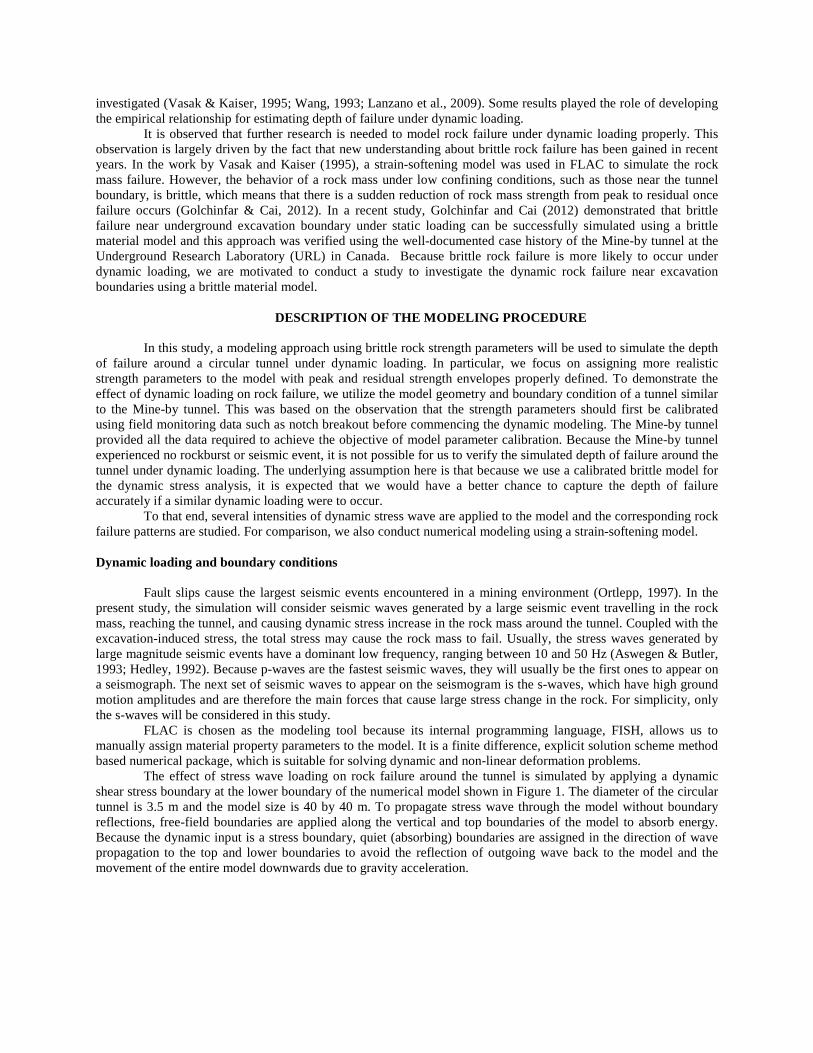
combination of static and dynamic stresses will induce maximum tangential stresses at locations A and B indicated in the figure.

Figure 2: The synthetic stress wave form used in this study.

An elastic stress analysis is conducted first for an in-situ stress field of 1σ = 60, 2σ = 45, and 3σ = 11

MPa. 2σ is parallel to the tunnel axis, and 1σ and 3σ are oriented in the x and y directions, respectively. Under this

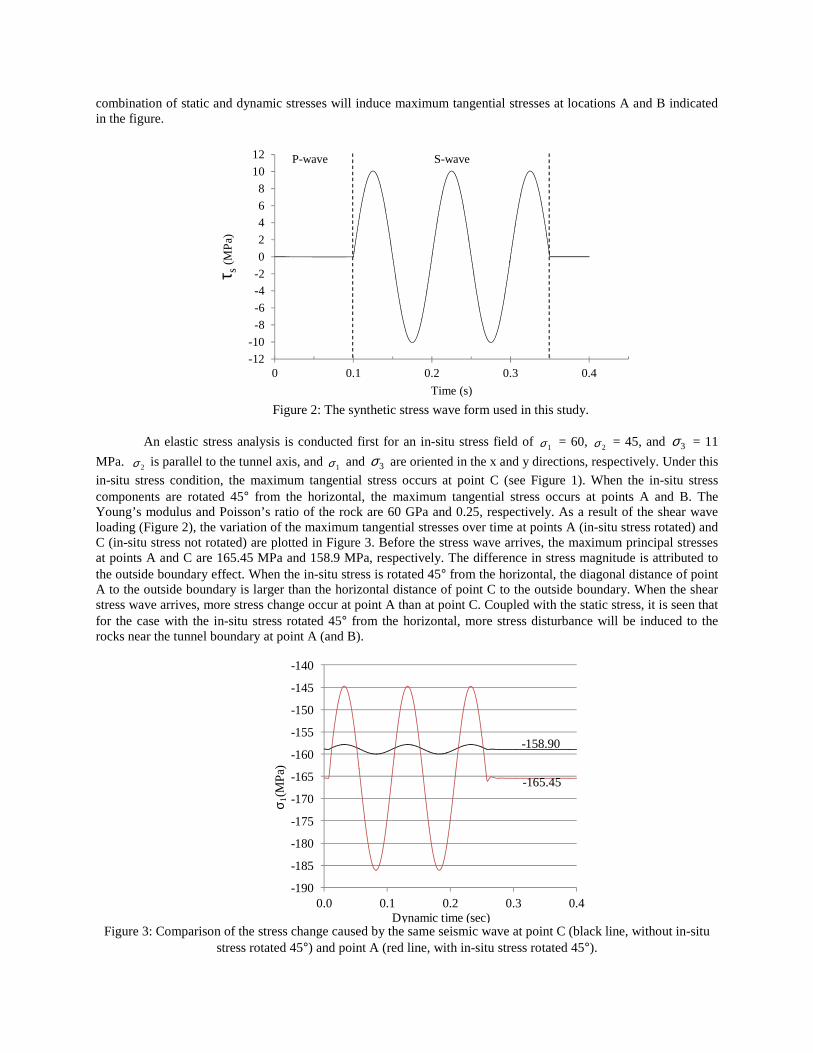
in-situ stress condition, the maximum tangential stress occurs at point C (see Figure 1). When the in-situ stress components are rotated 45° from the horizontal, the maximum tangential stress occurs at points A and B. The Young’s modulus and Poisson’s ratio of the rock are 60 GPa and 0.25, respectively. As a result of the shear wave loading (Figure 2), the variation of the maximum tangential stresses over time at points A (in-situ stress rotated) and C (in-situ stress not rotated) are plotted in Figure 3. Before the stress wave arrives, the maximum principal stresses at points A and C are 165.45 MPa and 158.9 MPa, respectively. The difference in stress magnitude is attributed to the outside boundary effect. When the in-situ stress is rotated 45° from the horizontal, the diagonal distance of point A to the outside boundary is larger than the horizontal distance of point C to the outside boundary. When the shear stress wave arrives, more stress change occur at point A than at point C. Coupled with the static stress, it is seen that for the case with the in-situ stress rotated 45° from the horizontal, more stress disturbance will be induced to the rocks near the tunnel boundary at point A (and B).

Figure 3: Comparison of the stress change caused by the same seismic wave at point C (black line, without in-situ

stress rotated 45°) and point A (red line, with in-situ stress rotated 45°).

-12

-10

-8

-6

-4

-2

0

2

4

6

8

10

12

0 0.1 0.2 0.3 0.4

τ s(M

Pa)

Time (s)

P-wave S-wave

-158.90

-165.45

-190

-185

-180

-175

-170

-165

-160

-155

-150

-145

-140

0.0 0.1 0.2 0.3 0.4

σ 1(M

Pa)

Dynamic time (sec)

Wave transmission through the model

As explained above, the dynamic loading is a sinusoidal shear stress wave applied at the base of the model

in the x-direction. The magnitude of the stress wave is a function of ppv (see Eq. (1)) and the wave frequency is 10 Hz. For the given rock, the shear wave velocity calculated from Eq. (3) is 3098 m/s. The largest zone dimension (∆l) of the numerical model is 0.1 m. The relation between the longest wave length (λ) and the maximum frequency is:

l

CCf ss

∆==

10λ

(4)

Using Eq. (4), we find that the maximum frequency which can be modeled accurately is over 3000 Hz.

Therefore the current zone (mesh) size is small enough to allow wave at the input frequency (10 Hz) to propagate accurately in the model. In addition, to increase the accuracy of the dynamic analysis, the mesh needs to be as uniform as possible throughout the model. The mesh used for the dynamic modeling in this study is shown in Figure 4.

Figure 4: The uniform fine mesh utilized in this modeling approach

DYNAMIC RESPONSE Two scenarios of rock failure are considered in the study. In the first scenario, rock failure in the form of

notch breakout occurred under static stress loading. The incoming dynamic stress wave further expands the failure zone. In the second scenario, the rock strength is higher than the maximum stress under static loading on the tunnel boundary. Hence, no failure will occur when the tunnel is excavated. When the dynamic stress wave is applied to the model, a dynamic stress increase will be generated in the rock around the tunnel. If the combined stress (static plus dynamic stresses) is high enough, failure will occur around the tunnel.

It is understood that the material properties under dynamic loading are different from those under static loading. Rock strength is generally higher under dynamic loading than under static loading (Olsson, 1991; Cai et al., 2007). However, the loading rate of the dynamic stress generated by a seismic event (or ppv) is not high. For simplicity we assume that the same peak and residual rock strength envelopes calibrated under static loading are applicable to dynamic loading.

Deepening of depth of failure by dynamic loading

From back analyses of well-documented case histories, we have built confidence on modeling brittle rock

failure under static stress loading (Golchinfar & Cai, 2012; Diederichs, 2007; Edelbro, 2010). In the present study, we will first simulate the extension of the notch failure of the tunnel under dynamic stress loading. The purpose is to use a calibrated model to understand how the rock will respond under dynamic loading, which can be generated by

-8.000

-6.000

-4.000

-2.000

0.000

2.000

4.000

6.000

8.000

-8.000 -6.000 -4.000 -2.000 0.000 2.000 4.000 6.000 8.000

40 m

40 m

fault-slip induced by rockbursts or natural earthquakes. The insight gained from such a failure process analysis will assist us to design better rock support systems for underground construction.

The modeling procedure is as follows. First, we run the model under static loading and let the model reach equilibrium. A static equilibrium can be obtained only if sufficient cycling steps are taken. In general, about 50,000 cycling steps are required before the unbalanced force reaches an insignificant value. This is especially important in an analysis in which rock failure occurs. The failure zone around the tunnel is plotted and compared with the field observation data. The model parameters are adjusted to match the modeling results to the field observation.

Next, we initiate the dynamic analysis and run the model until the stress wave input is finished, then further run the model until the stress wave passes the top boundary. Failure due to dynamic loading is then analyzed. The material parameters are listed in Table 1. For comparison, we conducted numerical modeling using both the brittle and the strain-softening models. The tensile strength and dilation angle are 30 MPa and 30 degrees, respectively.

Table 1: Peak and residual strength parameters for both the brittle and strain-softening models

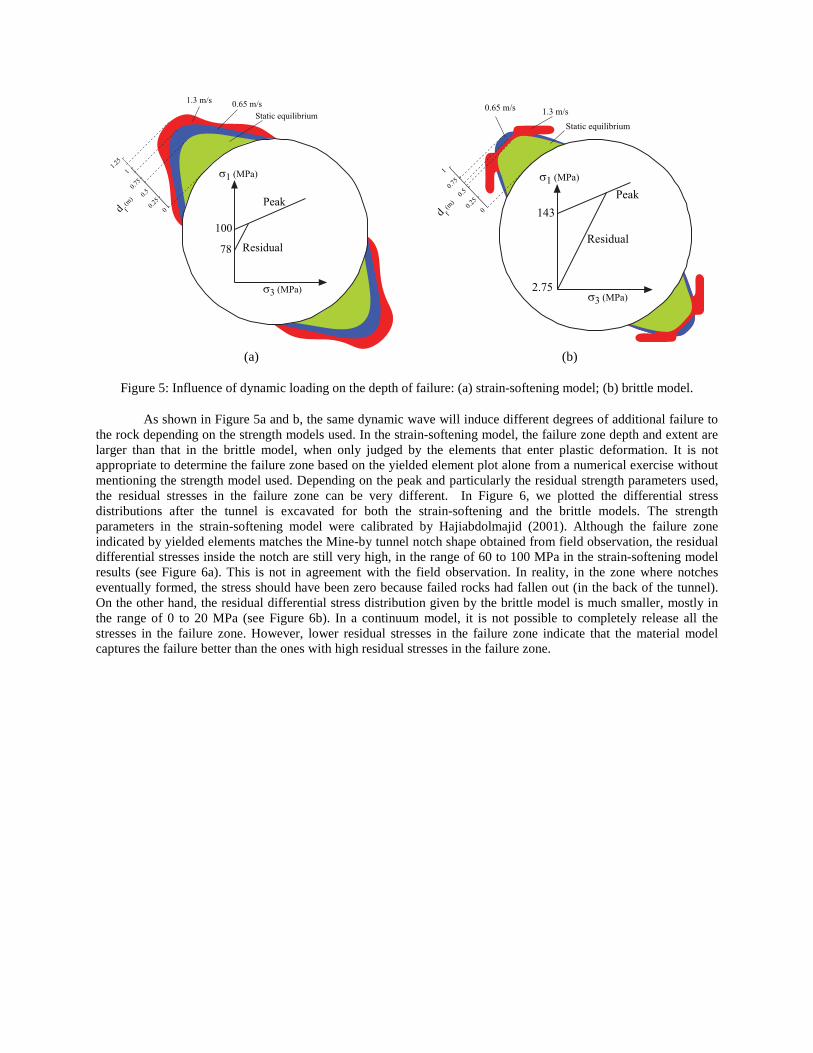
Under static loading with an in-situ stress field of 1σ = 60 MPa and 3σ = 11 MPa, where 1σ is rotated 45°

from horizontal, the failure zones around the tunnel when the tunnel is excavated are plotted with green filling in Figure 5a and b, for the strain-softening and the brittle material models, respectively. The peak and residual strength envelopes of the two models are shown as inserts in the figures. The peak and residual uniaxial compressive strengths of the strain-softening model and the brittle model are 100 MPa and 78 MPa, 143 MPa and 2.75 MPa, respectively. In the strain-softening model, the characteristic strains for cohesion and friction angle are 0.2% and 0.5%, respectively. As discussed in Golchinfar and Cai (2012), the brittle rock model is more appropriate for simulating brittle rock failure because for fractured rocks, the residual strength is purely frictional strength.

The 10 Hz frequency sinusoidal shear waves with two stress intensities (ppv = 0.65 and 1.3 m/s) are applied to the model which has been in equilibrium statically. In this case, notch failure has already occurred under static loading. Hence, the dynamic stress wave loading will increase the failure zone. The failure zone increases are shown in Figure 5 by blue and red colors for the wave intensities of ppv = 0.65 m/s and 1.3 m/s, respectively. The stronger shear wave indicated with the red zone extends further over the blue zone in Figure 5a, where a strain-softening material is used. In Figure 5b, where the brittle material model with parameters specified in Table 1 is used, the red zone extends differently compared with that in the strain-softening material.

Brittle Strain-softening

c (MPa), εp (%) 60, 10-10 50, 0.2

φ (°), εp (%) 10, 10-10 0, 0.5

c (MPa), εp (%) 0.5, 10-10 15, 0.2

φ (°), εp (%) 50, 10-10 48, 0.5

Pe

ak

Re

sid

ua

l

(a) (b)

Figure 5: Influence of dynamic loading on the depth of failure: (a) strain-softening model; (b) brittle model.

As shown in Figure 5a and b, the same dynamic wave will induce different degrees of additional failure to the rock depending on the strength models used. In the strain-softening model, the failure zone depth and extent are larger than that in the brittle model, when only judged by the elements that enter plastic deformation. It is not appropriate to determine the failure zone based on the yielded element plot alone from a numerical exercise without mentioning the strength model used. Depending on the peak and particularly the residual strength parameters used, the residual stresses in the failure zone can be very different. In Figure 6, we plotted the differential stress distributions after the tunnel is excavated for both the strain-softening and the brittle models. The strength parameters in the strain-softening model were calibrated by Hajiabdolmajid (2001). Although the failure zone indicated by yielded elements matches the Mine-by tunnel notch shape obtained from field observation, the residual differential stresses inside the notch are still very high, in the range of 60 to 100 MPa in the strain-softening model results (see Figure 6a). This is not in agreement with the field observation. In reality, in the zone where notches eventually formed, the stress should have been zero because failed rocks had fallen out (in the back of the tunnel). On the other hand, the residual differential stress distribution given by the brittle model is much smaller, mostly in the range of 0 to 20 MPa (see Figure 6b). In a continuum model, it is not possible to completely release all the stresses in the failure zone. However, lower residual stresses in the failure zone indicate that the material model captures the failure better than the ones with high residual stresses in the failure zone.

0

11.

25

0.75

d f (m

)0.

5

0.25

Static equilibrium

0.65 m/s1.3 m/s

Peak

100

Residual78

σ1 (MPa)

σ3 (MPa)

0

1

0.75

0.5

0.25

Static equilibrium

Peak

143

Residual

σ1 (MPa)

σ3 (MPa)2.75

1.3 m/s0.65 m/s

d f (m

)

(a) (b)

Figure 6: 31 σσ − stress distribution in the rock when the notches are formed under static stress loading: (a) strain-

softening model, (b) brittle model.

The dynamic loading of a seismic wave further increases the stress in the rock. In the strain-softening model, the stresses in the notch failure zone (under static loading) are high. Therefore, elements just outside the notch boundary can carry high stresses and this makes it easier for these elements to fail under additional dynamic loading, leading to failure zone expansion as shown in Figure 5a. In the brittle model, on the other hand, the stress concentration zone is located at the tip of the notch failure zone (see Figure 6b) and additional stress increase induced by the seismic wave will cause additional failure in the highly stressed areas. When ppv is equal to 0.65 m/s, the shape of the additional failure zone due to dynamic loading is similar to that in the strain-softening model, but the depth of failure is smaller. For ppv = 1.3 m/s, wing-shaped failure zones are created by the dynamic loading in the brittle model, which is different from that in the strain-softening model (red and blue areas in Figure 5).

Creation of rock failure due to subsequent dynamic loading

In many underground openings and mines, tunnels were stable after excavation because the rock strength

was higher than the maximum excavation or mining-induced stress. However, when a fault-slip event occurred, the seismic wave could cause rock failure in tunnels located away from the seismic source. In the following discussion, we study rock failure in a tunnel located in a weaker rock with a different in-situ stress field from the previous example. The peak and residual strength parameters of both the brittle and strain-softening models are presented in Table 2. The model parameters are chosen in such a way that upon the tunnel excavation, there will be no rock failure. Rock failure is only induced by subsequent dynamic loading. In the example shown above, the ratio of the principal in-situ stresses (Ko ratio) is 5, which is extremely high. For this simulation,

1σ = 30 MPa and 3σ = 15

MPa (Ko = 2) are used. Again, to maximize the stress increase due to dynamic stress loading, the maximum principal stress is rotated 45° from the horizontal. The shear stress wave is applied to the bottom boundary of the model (Figure 1).

σ1-σ3 (MPa)

0 20 40 60 80

100 120

140 160

Table 2: Strength parameters for the brittle and strain-softening models

Figure 7 presents the differential stress distributions and the failure zone distribution in the rock for the brittle and the strain-softening models. As expected, no rock failure occurs under static loading using either modeling approach, which means that after tunnel excavation, the maximum tangential stress at the tunnel wall is less than the wall strength of 62 MPa. Under dynamic loading, new rock failure zones are formed in the direction in which the combined tangential stress is the maximum. The depth of failure is higher for the case with higher dynamic stress increase (Figure 7).

Figure 7 shows that when the peak and residual strengths of the brittle and strain-softening models are the same (see Table 2), respectively, the depth of failure zone by the brittle model is similar to that of the strain-softening model while the extent is larger. On the other hand, the results shown in Figure 5 indicate that the failure zone by the strain-softening model is larger than that by the brittle model. This is because that the peak and residual strengths in these two models are different. The peak strength of the strain-softening model in Figure 5 is lower than that of the brittle model, while the residual strength of the strain-softening model is higher.

Bri

ttle

mo

del

Str

ain

-so

ften

ing

mo

del

Static ppv = 0.65 m/s ppv = 1.3 m/s

Figure 7: Depth of failure under static and dynamic loading for brittle and strain-softening models.

Brittle Strain-softening

c (MPa), εp (%) 26, 10-10 26, 0.2

φ (°), εp (%) 10, 10-10 10, 0.5

c (MPa), εp (%) 0.5, 10-10 0.5, 0.2

φ (°), εp (%) 50, 10-10 50, 0.5

Pe

ak

Re

sid

ua

l

σ1-σ

3 (MPa)

0 10

20 30

40 50

σ1-σ

3 (MPa)

0 10

20 30

40 50

Kaiser et al. (1996) presented a chart which plots the normalized depth of failure (df/a) as a function of normalized tangential wall stress to the uniaxial compressive strength of the original rock (σmax/σc) and ppv. Here, a is the radius of the tunnel, σmax is maximum tangential stress, and σc is the strength of the rock mass. When the stress to strength ratio σmax/σc and ppv are known, the depth of failure due to dynamic loading can be estimated using the chart.

Based on the numerical modeling results, we plot a few contour lines relating depth of failure to the stress to strength ratio and ppv in Figure 8 for the strain-softening (blue lines and blue markers) and the brittle models (red lines and red markers). The empirical static contour line given by Kaiser et al. (1996) is shown in Figure 8 as a solid black line.Under static loading (ppv = 0), the depth of failure predicted by both models is in reasonable agreement with that of the empirical relation given by Kaiser et al. (1996). Although there are some differences between the results of the strain-softening and the brittle models, the differences are nevertheless small when the stress to strength ratio is low (σmax/σc = 1).

Figure 8: Comparison of the simulated depth of failure by a brittle model (red lines and markers) and a strain-softening model (blue lines and markers)

Under dynamic loading, when the stress-to-strength ratio is high, the slopes for the depth of failure contours by the numerical modeling vary depending on the material’s post-peak behavior and the intensity of input dynamic wave. For example, when the stress to strength ratio is higher than 1, the strain-softening model predicts a larger depth of failure than the brittle model, under ppv = 0.65 m/s dynamic loading (thick solid lines). On the other hand, the depth of failure under ppv = 1.3 m/s dynamic loading (dashed lines) shows a steady rise with increasing stress-to-strength ratio, regardless of the post-peak behavior of the rock.

SUMMARY

A parametric study with two different intensities of input stress wave was carried out, employing both the

brittle and the strain-softening models. For each case, the dynamic depth of failure was plotted as a function of the ratio of maximum tangential stress to the rock mass strength as well as the dynamic stress wave intensity expressed by the peak particle velocity. By comparing the numerically simulated depths of failure under dynamic loading, we noted that: • The simulated depth of failure depends on the material model used as well as the strength parameters. Both the

brittle and the strain-softening models can be used to simulate rock failure under dynamic loading. When both the peak and residual strengths are the same in the brittle and strain-softening models, the depth of failure by the brittle model is larger than that of the strain-softening model. However, the depth of failure given by the brittle model with a high peak strength and a low residual strength can be smaller than that given by the strain-softening model with a low peak strength and a very high residual strength. Therefore, judging the depth of

Empirical static

0.0

0.2

0.4

0.6

0.8

1.0

1.2

1.0 1.2 1.4 1.6 1.8

d f /a

σσσσ max/ σσσσc

failure only by the yielded elements in the numerical model can be misleading. One needs to examine the type of strength model used and the strength parameters applied.

• Under static stress loading conditions, the depths of failure given by the current numerical model with the calibrated material parameters are in reasonable agreement with those given by the empirical relations, regardless of the post-peak behavior of the rock.

• Under dynamic stress loading conditions, when the stress to strength ratio is as low as unity and when the peak and residual strengths are the same in both brittle and strain-softening models, the difference between numerically simulated depths of failure, using either modeling approach is minimal. Only when the stress to strength ratio is high, do the dynamic depths of failure follow different increment trends depending on the intensity of input dynamic wave and the post-peak behavior model.

• Because of the discrepancy identified, we recommend that further research is needed to collect field data with ground motion and failure monitoring to verify the numerical simulation and empirical results.

ACKNOWLEDGMENT Financial supports from NSERC, Laurentian University, CEMI, MIRARCO, LKAB, VALE, and the

William Shaver Masters Scholarship in Mining Health and Safety are greatly appreciated.

REFERENCES Aswegen, G. & Butler, A.G., 1993. Applications of quantitative seismology in South African gold mines. In Young,

R.P., ed. In Proceedings of Rockbursts and Seismicity in Mines, Kingston. Balkema, Rotterdam, 1993. Cai, M., Kaiser, P.K. & Duff, D.J., 2012. Rock support design in burst-prone ground utilizing an interactive design

tool. Chicago: ARMA-American Rock Mechanics Association. Cai, M., Kaiser, P.K., Suorineni, F. & Su, K., 2007. A study on the dynamic behavior of the Meuse/Haute-Mame

Argillite. Physics and Chamistry of the earth, 32(8), pp.907-9016. Diederichs, M.S., 2007. Mechanistic interpretation and practical application of damage and spalling prediction

criteria for deep tunnelling. Canadian Geotechnical Journal, 44(9), pp.1082-116. Edelbro, C., 2010. Different approaches for simulating brittle failure in two hard rock mass cases: A parametric

study. Rock Mechanics and Rock Engineering, 43(2), pp.151-65. Golchinfar, N. & Cai, M., 2012. Modeling depth of failure using brittle mohr-coulomb failure model. In 21st

Canadian Rock Mechanics Symposium. Edmonton, Alberta, 2012. Hajiabdolmajid, V.R., 2001. Mobilization of Strength in Brittle Failure of Rock. Ph.D. thesis. Kingston, Ontario,

Canada: Queen's Univeristy. Hajiabdolmajid, V., Kaiser, P.K. & Martin, C.D., 2002. Modelling brittle failure of rock. International Journal of

Rock Mechanics and Mining Sciences, 39(6), pp.731-41. Hedley, D.G.F., 1992. Rockburst Handbook for Ontario Hardrock Mines. CANMET Special Report SP92-1E. Hoek, E. & Bieniawski, Z.T., 1965. Brittle fracture propagation in rock under compression. International journal of

fracture mechanics, 3(1), pp.137-55. Hoek, E., Kaiser, P.K. & Bawden, W.F., 1995. Support of Underground Excavations in Hard Rock. 3rd ed.

Rotterdam, Balkema: Taylor & Francis. Itasca, 2002. FLAC Manual. Minneapolis, MN, USA. Kaiser, P.K. et al., 2000. Underground works in hard rock tunneling and mining. International Conference on

Geotechnical and Geological Engineering, pp.841-926. Kaiser, P., Dwayne, D.T. & McCreath, D., 1996. Drift support in burst-prone ground. CIM bulletin, 89(998),

pp.131-38. Lanzano, G. et al., 2009. Experimental assessment of performance-based methods for the seismic design of circular

tunnels. In International Conference on Performance-Based Design in Earthquake Geotechnical Engineering., 2009.

Martin, C.D., Kaiser, P.K. & McCreath, D.R., 1999. Hoek-Brown parameters for predicting the depth of brittle failure around tunnels. Canadian Geotechnical Journal, 36(1), pp.136-51.

Olsson, W.A., 1991. The compressive strength of tuff as a function of strain rate from 10e-6 to 10e3 sec. International journal of rock mechanics and mining sciences, 28, pp.115-18.

Ortlepp, W.D., 1997. Rock fracture and rockbursts – an illustrative. Owen, G.N. & Scholl, R.E., 1981. Earthquake engineering of large underground structures. Final Report. San

Francisco, CA: URS/Blume (John A.) Federal Highway Administration and National Science.

Stacey, T.R. & Ortlepp, W.D., 1993. Rockburst mechanisms and tunnel support in rockburst conditions. In Proceedings of International Conference in Geomechanics. Ostrava, Czech Republic, 1993.

Vasak, P. & Kaiser, P.K., 1995. Tunnel stability assessment during rockbursts. Montreal, Quebec: CAMI 95, 3rd Canadian Conference on Computer Applications in the Mineral Industry.

Wang, J.-N.J., 1993. Seismic Design of Tunnels- a simple state of-the-art design approach. 1st ed. New York, New York: Parsons Brinckerhoff Inc.