Numerical Methods - Initial Value Problems for...

Numerical Methods -Initial Value Problems for ODEs

Y. K. Goh

Universiti Tunku Abdul Rahman

2013

Y. K. Goh (UTAR) Numerical Methods - Initial Value Problems for ODEs 2013 1 / 43

Outline

1 Initial Value Problems & ODEs

2 Single Step MethodsEuler’s MethodTaylor Series Method of Order nRunge-Kutta MethodAdaptive Runge-Kutta-Fehlber Method

3 Multistep MethodsAdams-Bashforth Explicit MethodsAdams-Mouton Implicit MethodsPredictor-Corrector Methods

4 Convergence and StabilityConvergenceStability Function

5 Higher Order ODE


Initial Value Problems & ODEs

Definition (Ordinary Differential Equation (ODE))

An ordinary differential equation is an equation that involves one or morederivatives of an univariate function.

The solutions for an ODE are differ from each other by a constant.

Definition (Initial Value Problem)

A solution to the initial value problem (IVP)

dy

dt= f(t, y), with y(t0) = y0

on an interval [t0, b] is a differential function y = φ(t) such that φ(t0) = y0 andφ′(t) = f(t, φ(t)) for all t ∈ [t0, b]

The solution of IVP is unique.


Well-posed Problem

Theorem (Well-posed problem)

Suppose that D = {(t, y)|a ≤ t ≤ b and −∞ < y <∞} and that f(t, y) iscontinuous on D. If f satisfies a Lipschitz condition on D, then the initial valueproblem

y(t) = f(t, y), a ≤ t ≤ b, y(a) = y0,

has a unique solution.

Definition (Lipschitz condition)

A function f(t, y) is said to satisfy a Lipschitz condition in the variable y on a setD ⊂ R2 if there exist a constant L > 0 such that

|f(t, y1)− f(t, y2)| < L|y1 − y2|,

whenever (t, y1) and (t, y2) are in D. The constant L is called a Lipschitzconstant for f .


Well-posed Problem

Theorem

Suppose f(t, y) is defined on a convex set D ⊂ R2. If there exists a constantL > 0, such that

|∂f∂y

(t, y)| ≤ L, for all (t, y) ∈ D,

then f satisfies a Lipschitz condition on D in the variable y with Lipschitzconstant L.

Example

Show that there is a unique solution to the initial value problem

y′(t) = 1 + t sin(yt), 0 ≤ t ≤ 2, y(0) = 0.


Outline





5 Higher Order ODE


Euler’s Method

Euler’s method is the simplest numerical method for solving well-posed IVP:

dy

dt= f(t, y), a ≤ t ≤ b, y(a) = α.

First partition / discretise the interval into N +1 equally spaced mesh points:a = t0 < t1 < t2 < · · · < tN = b, ti = t0 + ih, i ≤ N and h = (b− a)/N.Consider the two adjecent mesh points [ti, ti+1], from the Taylor’s series,

y(ti+1) = y(ti + h) = y(ti) + hy′(ti) +h2

2y′′(ξ), ξ ∈ [ti, ti+1].

Write yi as the approximation to the actual solution y(ti) and substitutey′(ti) = f(ti, y(ti)), we have the Euler’s method iteration rule:

yi+1 = yi + hf(ti, yi).

The initial starting point of the Euler’s method is given by the initialcondition y0 = y(a) = α.


Euler’s Method

The local discretisation error εi = |y(ti + h)− y(ti)− hf(ti, y(ti))| is O(h2).However, the global discretisation error Ei = |y(ti)− yi| is O(h).

Example

Solve the IVP y′ = (t− y)/2 with y(0) = 1 over 0 ≤ t ≤ 3 with Euler method.ANSWER: MATLAB code : nm06_euler_driver.m

(Analytic solution is 3e−t/2 − 2 + t)


Outline





5 Higher Order ODE


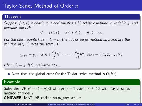
Taylor Series Method of Order n

Theorem

Suppose f(t, y) is continuous and satisfies a Lipschitz condition in variable y, andconsider the IVP

y′ = f(t, y), a ≤ t ≤ b, y(a) = α.

For the mesh points ti+1 = ti + h, the Taylor series method approximate thesolution y(ti+1) with the formula:

yi+1 = y0 + d1h+d22!h2 + · · ·+ dn

n!hn, for i = 0, 1, 2, . . . , N,

where di = y(i)(t) evaluated at ti.

Note that the global error for the Taylor series method is O(hn).

Example

Solve the IVP y′ = (t− y)/2 with y(0) = 1 over 0 ≤ t ≤ 3 with Taylor seriesmethod of order 2.ANSWER: MATLAB code : nm06_taylor2.m


Outline





5 Higher Order ODE


Runge-Kutta Method of Order 2

The methods tried to imitate the Taylor series method without requiringanalytic differentiation of the ODE.

In Euler method: yi+1 = yi + hf(ti, yi), the slope f(t, y) is evaluated at thestart of the interval ti, ie a forward difference scheme.

Intuitively, for better accuracy, we could evaluate f(t, y) at the midpoint byusing the Euler method first to obtain yi+h/2, then evaluate f(ti+h/2, yi+h/2)to get a symmetrical scheme.

Because of the symmetry, the local error is reduced by an order (in the stepsize) and the method is now a second-order method called Runge-KuttaMethod of order 2 (RK2) or the midpoint method.

The RK2 algorithm:

k1 = hf(ti, yi)

yi+1/2 = yi + k1/2

k2 = hf(ti+1/2, yi+1/2)

yi+1 = yi + k2


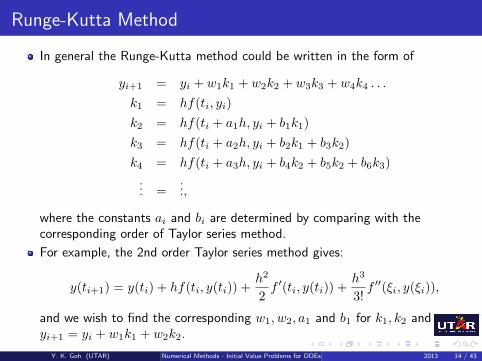
Runge-Kutta Method

In general the Runge-Kutta method could be written in the form of

yi+1 = yi + w1k1 + w2k2 + w3k3 + w4k4 . . .

k1 = hf(ti, yi)

k2 = hf(ti + a1h, yi + b1k1)

k3 = hf(ti + a2h, yi + b2k1 + b3k2)

k4 = hf(ti + a3h, yi + b4k2 + b5k2 + b6k3)

... =...,

where the constants ai and bi are determined by comparing with thecorresponding order of Taylor series method.

For example, the 2nd order Taylor series method gives:

y(ti+1) = y(ti) + hf(ti, y(ti)) +h2

2f ′(ti, y(ti)) +

h3

3!f ′′(ξi, y(ξi)),

and we wish to find the corresponding w1, w2, a1 and b1 for k1, k2 andyi+1 = yi + w1k1 + w2k2.


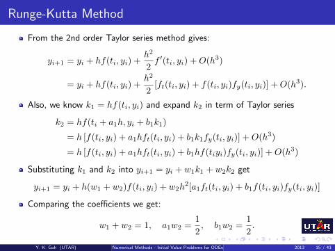
Runge-Kutta Method

From the 2nd order Taylor series method gives:

yi+1 = yi + hf(ti, yi) +h2

2f ′(ti, yi) +O(h3)

= yi + hf(ti, yi) +h2

2[ft(ti, yi) + f(ti, yi)fy(ti, yi)] +O(h3).

Also, we know k1 = hf(ti, yi) and expand k2 in term of Taylor series

k2 = hf(ti + a1h, yi + b1k1)

= h [f(ti, yi) + a1hft(ti, yi) + b1k1fy(ti, yi)] +O(h3)

= h [f(ti, yi) + a1hft(ti, yi) + b1hf(tiyi)fy(ti, yi)] +O(h3)

Substituting k1 and k2 into yi+1 = yi + w1k1 + w2k2 get

yi+1 = yi + h(w1 + w2)f(ti, yi) + w2h2[a1ft(ti, yi) + b1f(ti, yi)fy(ti, yi)]

Comparing the coefficients we get:

w1 + w2 = 1, a1w2 =1

2, b1w2 =

1

2.


Runge-Kutta Method

Note the there are 3 equations for the four unknown w1, w2, a1 and b1,therefore we have one degree of freedom in solving the coefficients.

Choose w1 = 0, w2 = 1, a1 = b1 = 12 we have the mid-point method:

k1 = hf(ti, yi)

k2 = hf(ti + h/2, yi + k1/2)

yi+1 = yi + k2

It is possible to choose an optimal value for a1 such that the error O(h3) isminimized. The value chosen is a1 = 2

3 and thus w1 = 14 , w2 = 3

4 , b1 = 23 :

k1 = hf(ti, yi)

k2 = hf(ti +2

3h, yi +

2

3k1)

yi+1 = yi +1

4k1 +

3

4k2


Runge-Kutta Method of Order 4

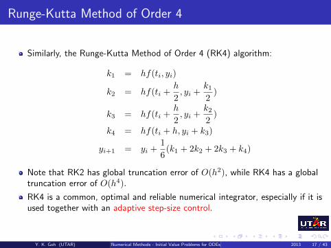
Similarly, the Runge-Kutta Method of Order 4 (RK4) algorithm:

k1 = hf(ti, yi)

k2 = hf(ti +h

2, yi +

k12)

k3 = hf(ti +h

2, yi +

k22)

k4 = hf(ti + h, yi + k3)

yi+1 = yi +1

6(k1 + 2k2 + 2k3 + k4)

Note that RK2 has global truncation error of O(h2), while RK4 has a globaltruncation error of O(h4).

RK4 is a common, optimal and reliable numerical integrator, especially if it isused together with an adaptive step-size control.


Outline





5 Higher Order ODE


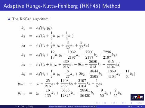
Adaptive Runge-Kutta-Fehlberg (RKF45) Method

The RKF45 algorithm:

k1 = hf(ti, yi)

k2 = hf(ti +1

4h, yi +

1

4k1)

k3 = hf(ti +3

8h, yi +

3

32k1 +

9

32k2)

k4 = hf(ti +12

13h, yi +

1932

2197k1 −

7200

2197k2 +

7296

2197k3)

k5 = hf(ti + h, yi +439

216k1 − 8k2 +

3680

513k3 −

845

4104k4)

k6 = hf(ti +1

2h, yi −

8

27k1 + 2k2 −

3544

2565k3 +

1859

4104k4 −

11

40k5)

yi+1 = yi +25

216k1 +

1408

2565k3 +

2197

4104k4 −

1

5k5

yi+1 = yi +16

135k1 +

6656

12825k3 +

28561

56430k4 −

9

50k5 +

2

55k6


Adaptive Runge-Kutta-Fehlberg (RKF45) Method

The RKF45 algorithm gives two estimates for y(ti), ie:

4th order estimate : yi+1; and5th order estimate : yi+1.

The difference between the two estimates gives the local truncation error. ie.ε = |yi+1 − yi+1| ∼ O(h5).

A simple adaptive scheme:

Choose an acceptable error ε0.Suppse we did a calculation with step size hc and error εc, then a newstep-size that will produce error ε0 is h0 = hc(ε0/εc)

1/5. Hence,If εc ≤ ε0, accept the calculation with current step-size hc, but change thenext step size to h0.If εc > ε0, reject yi+1 and repeat the calculation with step-size h0.

The Matlab command ode45 implement a variant of RK45 with adaptivestep control.


Outline





5 Higher Order ODE


Multistep Methods

Multistep methods make use of the information from several previous meshpoints to compute the value at the new mesh point.

Consider y′(t) = f(t, y), integrate over [ti, ti+1] and we have:

y(ti+1) = y(ti) +

∫ ti+1

ti

f(t, y(t)) dt.

As y(ti+1) is unknown, we cannot evaluate the integral explicitly. Instead, werely on interpolating the integrand with a polynomial.

For example, let say we know the value of (ti, y(ti)) and we are approximatingf(t, y) with interpolating polynomial of degree 0 (ie a horizontal line), thenf(t, y) = f(ti, y(ti)) + (t− ti)f ′(τi, y(τi)) where τi ∈ [ti, ti+1].

Integrating over [ti, ti+1] and let h = ti+1 − ti, gives

y(ti+1) = y(ti) + hf(ti, y(ti)) +h2

2f ′(ξi, y(ξ)),

Which is the one-step Euler method

yi+1 = yi + hf(ti, yi).


Outline





5 Higher Order ODE


Adams-Bashforth Explicit Methods

Continue along the idea, now we use interpolating polynomial through thetwo points (ti, y(ti)) and (ti−1, y(ti−1)) for f(t, y):

y(ti+1) = y(ti) +

∫ ti+1

ti

{f(ti, y(ti)) + (t− ti)

f(ti, y(ti))− f(ti−1, y(ti−1))h

+(t− ti)(t− ti−1)

2!f ′′(τi, y(τi))

}dt

= y(ti) +h

2{3f(ti, y(ti))− f(ti−1, y(ti−1))}+

5

12h3f ′′′(ξi, y(ξi))

Two-step Adams-Bashforth method:

yi+1 = yi +h

2[3f(ti, yi)− f(ti−1, yi−1)] +

5

12h3f ′′′(ξi, y(ξi))


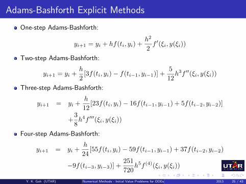
Adams-Bashforth Explicit Methods

One-step Adams-Bashforth:

yi+1 = yi + hf(ti, yi) +h2

2f ′(ξi, y(ξi))

Two-step Adams-Bashforth:

yi+1 = yi +h

2[3f(ti, yi)− f(ti−1, yi−1)] +

5

12h3f ′′(ξi, y(ξi))

Three-step Adams-Bashforth:

yi+1 = yi +h

12[23f(ti, yi)− 16f(ti−1, yi−1) + 5f(ti−2, yi−2)]

+3

8h4f ′′′(ξi, y(ξi))

Four-step Adams-Bashforth:

yi+1 = yi +h

24[55f(ti, yi)− 59f(ti−1, yi−1) + 37f(ti−2, yi−2)

−9f(ti−3, yi−3)] +251

720h5f (4)(ξi, y(ξi))


Outline





5 Higher Order ODE


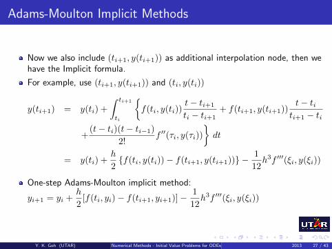
Adams-Moulton Implicit Methods

Now we also include (ti+1, y(ti+1)) as additional interpolation node, then wehave the Implicit formula.

For example, use (ti+1, y(ti+1)) and (ti, y(ti))

y(ti+1) = y(ti) +

∫ ti+1

ti

{f(ti, y(ti))

t− ti+1

ti − ti+1+ f(ti+1, y(ti+1))

t− titi+1 − ti

+(t− ti)(t− ti−1)

2!f ′′(τi, y(τi))

}dt

= y(ti) +h

2{f(ti, y(ti))− f(ti+1, y(ti+1))} −

1

12h3f ′′′(ξi, y(ξi))

One-step Adams-Moulton implicit method:

yi+1 = yi +h

2[f(ti, yi)− f(ti+1, yi+1)]−

1

12h3f ′′′(ξi, y(ξi))


Adams-Moulton Implicit Methods

One-step Adams-Moulton:

yi+1 = yi +h

2[f(ti+1, yi+1) + f(ti, yi)]−

1

12h3f ′′(ξi, y(ξi))

Two-step Adams-Moulton:

yi+1 = yi+h

12[5f(ti+1, yi+1)+8f(ti, yi)−f(ti−1, yi−1)]−

1

24h4f ′′′(ξi, y(ξi))

Three-step Adams-Moulton:

yi+1 = yi +h

24[9f(ti+1, yi+1) + 19f(ti, yi)− 5f(ti−1, yi−1)

+f(ti−2, yi−2)]−19

720h5f (4)(ξi, y(ξi))

Four-step Adams-Moulton:

yi+1 = yi +h

720[251f(ti+1, yi+1) + 646f(ti, yi)− 264f(ti−1, yi−1)

+106f(ti−2, yi−2)− 19f(ti−3, yi−3)]−3

160h6f (5)(ξi, y(ξi))


Outline





5 Higher Order ODE


Predictor-Corrector Methods

One weakness the Adams-Moulton implicit formula is it not always possibleto algebraically re-arrangethe formula to make y(ti+1) explicit.

However, combine with Adams-Bashforth explicit formula to form apredictor-corrector pairs.

The simplest example will be the so-called leapfrog algorithm:

Predictor (1-step AB) : pi+1 = yi + hf(ti, yi)Corrector (1-step AM) : yi+1 = yi +

h2[f(ti+1, pi+1) + f(ti, yi)]

Another commonly used method will be the 4th OrderAdams-Bashforth-Moulton methods:

Predictor : pi+1 = yi +h24[55fi − 59fi−1 + 37fi−2 − 9fi−3]

Corrector : yi+1 = yi +h2[9fi+1 + 19fi − 5fi−1 + fi−2], where

fi+1 = f(ti+1, pi+1)


Outline





5 Higher Order ODE


Convergence

Stability of ODE scheme depends on the nature of IVP.Eg, Euler scheme diverges for y′ = λy, y(0) = α, but converges for y′ = −λy.For convergent solution curves, the local errors at each step are reduced overt, and accumulative global error may be less than the sum of the local errors.

Theorem

For an initial value problem: y′ = f(t, y), y(0) = α

if fy > δ for some positive δ, then the solution curve diverges.

if fy < −δ, then the solution curve converges.


Outline





5 Higher Order ODE


Stability

Even if the IVP is convergent, it could still be unstable due to large h.

Example

Consider IVP y′ = (t− y)/2, y(0) = 1. We know that fy(t) = −1/2 for allt ∈ [0, 50], thus the Euler method should be convergent. However, the numericalsolution y(t) by using Euler method for for h = 2.5 is convergent but diverge forh = 5.


Stability

Consider a linear (or linearized) ODE: y′ = −λy, and discretized, say by Eulermethod (of course could be other method).

Then, we have yi+1 = yi − hλyi.The absolute stability function is defined as

Q(hλ) =

∥∥∥∥yi+1

yi

∥∥∥∥ .In the case for Euler method, we have Q(hλ) = (1− hλ).If the amplification factor Q(hλ) < 1, then we are guaranteed that thesequence {yi} will not grow without bound, and hence stable.

Assuming that λ is real, then for the Euler method to be stable we need−1 < 1− λh < 1 or 0 < λh < 2, ie h < 2/λ in order for the Euler method tobe stable.


Stability

The following figure shows an IVP (y′ = −10y, y(0) = 1) solved by Eulermethod with different values of step size h.Note that the numerical solution curves become unstable whenh ≥ 2/c = 0.10.


Outline





5 Higher Order ODE


Higher Order ODE & System of ODEs

Higher order ODE can be solved numerically by turning into a system of firstorder ODEs.

Consider IVP of order n:

y(n) = f(t, y, y′, . . . , y(n−1)), y(0) = α0, y′(0) = α1, . . . , y

(n−1) = αn−1.

Define new variables x1, x2, . . . , xn: x1 = y, x2 = y′, . . . , xn = y(n−1).

Now the IVP is equivalent to

x′1 = x2, x1(0) = α0

x′2 = x3, x2(0) = α1

...

x′n = f(t, x1, x2, . . . , xn), xn = αn−1

In vector notation: X′ = F(t,X), X(0) = A, where X = [x1, x2, . . . , xn]T ,

F = [x2, x3, . . . , f ]T and A = [α0, α1, . . . , αn−1].


System of First Order ODEs

Solve the system of first order ODEs numerically are very much like solving asingle first order ODEs.

For example, consider to solve X′(t) = F(t,X), X(0) = A with aRunge-Kutta method of order 4, we have

Discretise the time interval [a, b] into n subdivisions with h = (b− a)/n.RK4 iteration formula: Xi+1 = Xi +

h6[k1 + 2k2 + 2k3 + k4], where

k1 = hF(t,X)

k2 = hF(t+1

2h,X+

1

2k1)

k3 = hF(t+1

2h,X+

1

2k2)

k4 = hF(t+ h,X+ k3)


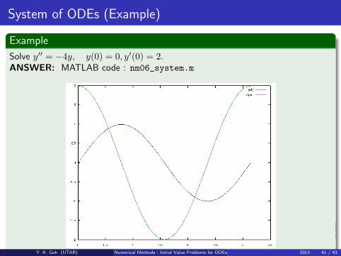
System of ODEs (Example)

Example

Solve y′′ = −4y, y(0) = 0, y′(0) = 2.ANSWER: MATLAB code : nm06_system.m


System of ODEs (Example)

Example (Lorenz system)

Solve the Lorenz system:x′ = σ(y − x)

y′ = x(ρ− z)− y

z′ = xy − βz

with the values σ = 3, ρ = 26.5 and β = 1.ANSWER: MATLAB code : nm06_lorenz.m


THE END


Numerical Methods - Initial Value Problems for...

Documents

Transcript of Numerical Methods - Initial Value Problems for...